1
HILINK REAL-TIME HARDWARE-IN-THE-LOOP CONTROL PLATFORM FOR MATLAB/SIMULINK User Manual release 1.5 May 1, 2011 Disclaimer The developers of the HILINK platform (hardware and software) have used their best efforts in the development. The developers make no warranty of any kind, expressed or implied, with regard to the developed hardware and software. The developers shall not be liable in any event for incidental or consequential damages in connection with or arising out of the performance or use of this hardware and software. The hardware and software are provided as-is and their users assume all risks and responsibility when using them. The hardware, software and this document are subject to change without notice. Brand names or product names are trademarks or registered trademarks of their respective owners. Copyright The HILINK platform (hardware and software) contains proprietary information protected by copyright. All rights reserved. No parts of the hardware, software and this document may be reproduced, ported, copied, distributed or translated in any form or by any means in whole or in part without the prior written consent of Zeltom LLC. c 2010 by Zeltom LLC web: http://zeltom.com email: [email protected] 47001 Harbour Pointe Ct. Belleville, MI 48111 USA CONTENTS 1. 2. 3. INTRODUCTION 1 1.1. Specifications . . . . . . . . . . . . . . . . . . . . . . . . . . . . . . . . . . . . . . 1 1.2. Requirements . . . . . . . . . . . . . . . . . . . . . . . . . . . . . . . . . . . . . . 2 1.3. Absolute Maximum Ratings . . . . . . . . . . . . . . . . . . . . . . . . . . . . . . 2 HARDWARE 3 2.1. Microcontroller . . . . . . . . . . . . . . . . . . . . . . . . . . . . . . . . . . . . . 4 2.2. Power Supply . . . . . . . . . . . . . . . . . . . . . . . . . . . . . . . . . . . . . . 4 2.3. Analog Inputs . . . . . . . . . . . . . . . . . . . . . . . . . . . . . . . . . . . . . . 5 2.4. Capture Inputs . . . . . . . . . . . . . . . . . . . . . . . . . . . . . . . . . . . . . . 5 2.5. Digital Inputs . . . . . . . . . . . . . . . . . . . . . . . . . . . . . . . . . . . . . . 6 2.6. Encoder Inputs . . . . . . . . . . . . . . . . . . . . . . . . . . . . . . . . . . . . . . 6 2.7. Analog Outputs . . . . . . . . . . . . . . . . . . . . . . . . . . . . . . . . . . . . . 7 2.8. Frequency Outputs . . . . . . . . . . . . . . . . . . . . . . . . . . . . . . . . . . . 7 2.9. Digital Outputs . . . . . . . . . . . . . . . . . . . . . . . . . . . . . . . . . . . . . 8 2.10. Pulse Outputs . . . . . . . . . . . . . . . . . . . . . . . . . . . . . . . . . . . . . . 8 2.11. Lowpass Filters . . . . . . . . . . . . . . . . . . . . . . . . . . . . . . . . . . . . . 9 2.12. H-bridges . . . . . . . . . . . . . . . . . . . . . . . . . . . . . . . . . . . . . . . . 9 2.13. Serial Communication . . . . . . . . . . . . . . . . . . . . . . . . . . . . . . . . . . 9 2.14. Power on Indicator and Reset . . . . . . . . . . . . . . . . . . . . . . . . . . . . . 10 SOFTWARE 11 3.1. Installation . . . . . . . . . . . . . . . . . . . . . . . . . . . . . . . . . . . . . . . . 11 3.2. Block Library . . . . . . . . . . . . . . . . . . . . . . . . . . . . . . . . . . . . . . 11 3.3. Analog Input Block . . . . . . . . . . . . . . . . . . . . . . . . . . . . . . . . . . . 12 3.4. Capture Input Block . . . . . . . . . . . . . . . . . . . . . . . . . . . . . . . . . . . 14 3.5. Digital Input Block . . . . . . . . . . . . . . . . . . . . . . . . . . . . . . . . . . . 15 3.6. Encoder Input Block . . . . . . . . . . . . . . . . . . . . . . . . . . . . . . . . . . 16 3.7. Analog Output Block . . . . . . . . . . . . . . . . . . . . . . . . . . . . . . . . . . 18 3.8. Frequency Output Block . . . . . . . . . . . . . . . . . . . . . . . . . . . . . . . . 20 4. 3.9. Digital Output Block . . . . . . . . . . . . . . . . . . . . . . . . . . . . . . . . . . 21 3.10. Pulse Output Block . . . . . . . . . . . . . . . . . . . . . . . . . . . . . . . . . . . 23 3.11. Filtered Pulse Outputs . . . . . . . . . . . . . . . . . . . . . . . . . . . . . . . . . . 25 3.12. H-bridge Outputs . . . . . . . . . . . . . . . . . . . . . . . . . . . . . . . . . . . . 26 3.13. Sampling Rate . . . . . . . . . . . . . . . . . . . . . . . . . . . . . . . . . . . . . . 27 3.14. Data Types . . . . . . . . . . . . . . . . . . . . . . . . . . . . . . . . . . . . . . . . 28 USAGE 29 4.1. Basic Inputs and Outputs . . . . . . . . . . . . . . . . . . . . . . . . . . . . . . . . 29 4.2. Filtering a Square Wave . . . . . . . . . . . . . . . . . . . . . . . . . . . . . . . . . 31 4.3. Generating a Nonstandard Wave . . . . . . . . . . . . . . . . . . . . . . . . . . . . 32 4.4. Switching Voltage Regulator . . . . . . . . . . . . . . . . . . . . . . . . . . . . . . 33 4.5. General Guidelines . . . . . . . . . . . . . . . . . . . . . . . . . . . . . . . . . . . 34 1. INTRODUCTION The HILINK platform offers a seamless interface between physical plants and Matlab/Simulink for implementation of hardware-in-the-loop real-time control systems. It is fully integrated into Matlab/Simulink and has a broad range of inputs and outputs. The platform is a complete and low-cost real-time control system development package for both educational and industrial applications. The HILINK platform consists of the real-time control board (hardware) and the associated Matlab interface (software). The hardware of the HILINK platform has 8×12 bit analog inputs, 2×16 bit capture inputs, 2 × 16 bit encoder inputs, 1 × 8 bit digital input, 2 × 12 bit analog outputs, 2 × 16 bit frequency outputs, 2 × 16 bit pulse outputs and 1 × 8 bit digital output. The board also contains 2 H-bridges with 5 A capability to drive external heavy loads. Some inputs and outputs are multiplexed to simplify the hardware. The board is interfaced to the host computer that runs Matlab through a serial port. The software of the HILINK platform is fully integrated into Matlab/Simulink/Real-Time Windows Target and comes with Simulink library blocks associated with each hardware input and output. The library contains Analog Input Block, Capture Input Block, Encoder Input Block, Digital Input Block, Analog Output Block, Frequency Output Block, Digital Output Block and Pulse Output Block. The platform achieves real-time operation with sampling rates up to 3.8 kHz. The HILINK platform has been developed to extend and optimize the real-time operation of Matlab, Simulink and Real-Time Windows Target. The developed platform is uniquely integrated into Matlab to achieve real-time operation in Matlab under Windows. The salient features of the HILINK platform make it ideal for implementation of hardware-in-the-loop real-time control systems in both educational and industrial applications. 1.1. Specifications • Power supply: 6 − 15 V, minimum 0.15 A, regulated • Interface: 115200 baud, 8 bit data, no parity, 1 stop bit • Analog inputs: A0–A7, 0 − 5 V analog, 12 bit resolution • Capture inputs: C0–C1, 0 − 5 V digital, 16 bit resolution • Digital inputs: D0 d0–D0 d7, 0 − 5 V digital, 8 lines • Encoder inputs: E0–E1, 0 − 5 V digital, 16 bit resolution • Frequency outputs: F0–F1, 0 − 5 V digital, 16 bit resolution 1 • Analog outputs: B0–B1, 0 − 5 V analog, 12 bit resolution • Digital outputs: G0 g0–G0 g7, 0 − 5 V digital, 8 lines • Pulse outputs: H0–H1, 0 − 5 V digital, 16 bit resolution • Filtered pulse outputs: L0–L1, 0 − 5 V analog • H-bridge outputs: P0–P1, 0−(supply voltage) V digital, 5 A • Voltage regulator output: VDD, 5 V, 0.25 A, regulated power supply • Ground: GND, 0 V • Sampling rate: up to 3.8 kHz 1.2. Requirements • PC with Windows XP or later and an available serial port or an expansion slot for a serial card • Serial crossover (null modem) cable • Matlab R2007b or later with Simulink, Real-Time Workshop and Real-Time Windows Target • HILINK hardware (real-time control board) 1.4 or later • HILINK software 1.4 or later • Power supply (regulated, 6 − 15 V and at least 0.15 A without any load) 1.3. Absolute Maximum Ratings • Power supply voltage: minimum 3 V, maximum 16 V • Each analog, digital, capture and encoder input: minimum −0.3 V, maximum +5.3 V • Each analog, digital, frequency and pulse output: minimum −25 mA, maximum +25 mA • Each filtered pulse output: minimum −25 mA, maximum +25 mA • Each H-bridge output: minimum −5 A, maximum +5 A • Total current from/into all inputs and outputs (except power supply, voltage regulator and H-bridges): minimum −200 mA, maximum +200 mA • Voltage regulator output: maximum 0.5 A (total) • Operating ambient temperature: minimum 10 ◦ C, maximum 50 ◦ C 2 2. HARDWARE The real-time control board is based on a dsPIC30F2012 digital signal controller. It has a total number of 8 × 16 bit inputs and 8 × 16 bit outputs capability. The inputs and outputs can be selected among the inputs and outputs listed above. The board is interfaced to the main computer that runs Matlab through a serial port. Two pulse-width modulation driven H-bridges with 5 A drive capability are included on the board to drive external actuators or loads. The functional block diagram of the board is shown in Figure 1, where A0–A7 are the analog inputs, B0–B1 are the analog outputs, C0–C1 are the capture inputs, D0 d0–D0 d7 are the digital inputs, E0–E1 are the encoder inputs, F0–F1 are the frequency outputs, G0 g0–G0 g7 are the digital outputs and H0–H1 are the pulse outputs; ADC represents the analog-to-digital converter, DAC represents the digital-to-analog converter, ICM represents the inputcapture module, OCM represents the output-compare module, DIP represents the digital-input port, DOP represents the digital-output port, QEM represents the quadrature-encoder module and PWM represents the pulse-width modulator; FLs are the lowpass filters with outputs L0–L1 and HBs are the H-bridges with outputs P0–P1; and µC is the central microcontroller, UART is the universal-asynchronous-receivertransmitter unit and PC is the host computer. PC C0 C1 D0 d7 E0 E1 ICM F0 F1 OCM µC ··· D0 d0 B0 B1 DAC ADC DIP QEM DOP PWM ··· A7 UART ··· A0 G0 g0 FL L0 FL L1 HB P0 HB P1 G0 g7 H0 H1 Figure 1. Functional block diagram of the board. The layout of the board is shown in Figure 2. The inputs and outputs are connected to the board through standard pin header type connectors. The pins of all connectors are clearly indicated on the board for convenience. Access to the on-board 5 V, 0.25 A voltage regulator output is also provided for external light power supply requirements. 3 Figure 2. Component layout of the board. 2.1. Microcontroller The real-time control board employs a dsPIC30F2012 digital signal controller for central control. The dsPIC30F2012 is a high performance 16 bit digital signal controller with 12 kB flash program memory and 1 kB SRAM data memory. It has also 3 × 16 bit timers/counters, 2 × 16 bit input-capture, 2 × 16 bit output-compare, 1 × SPI module, 1 × I2 C module, 1 × UART module, 1 × 12 bit analog-to-digital converter, 21 interrupt sources with 3 external interrupts, high current sink/source I/O pins, programmable low-voltage detection, programmable brown-out reset, power-on reset, power-up timer, oscillator start-up timer, watchdog timer, fail-safe clock monitor operation, in-circuit serial programming, selectable power management modes and 7.37 MHz internal RC oscillator with PLL. The microcontroller is set up to run from its internal oscillator at 7.37 × 106 × 16 = 117.92 MHz. 2.2. Power Supply The board requires a 6 − 15 V, at least 0.15 A (without any external load), regulated DC power supply to operate. The recommended power supply for the board is a 12 V well regulated DC power supply with 5 A drive capability. The power supply is connected to the board through the connector CON0. The pinout of CON0 is shown in Figure 3, where VPS is the positive terminal and GND is the negative (ground) terminal of the power supply. 4 GND VPS Figure 3. Power supply connector CON0. 2.3. Analog Inputs The board has 8 analog input channels A0–A7. Each analog input must be within 0− 5 V range analog signal. The connector CON1 provides access to each analog input channel. For convenience, GND and A0/D0 A1/D0 A2/D0 A3/D0 A4/D0 A5/D0 A6/D0 A7/D0 d0/G0 d1/G0 d2/G0 d3/G0 d4/G0 d5/G0 d6/G0 d7/G0 g0 g1 g2 g3 g4 g5 g6 g7 VDD are also provided with each channel. The pinout of CON1 is shown in Figure 4. GND VDD Figure 4. Analog inputs connector CON1. The value of each analog input is converted to its digital representation by the analog-to-digital converter. The sampling frequency of the analog-to-digital converter is 117.92 × 10⁶ /4096 = 28.7891 kHz. The resolution of the analog-to-digital converter is 12 bit. The analog inputs are multiplexed with the corresponding digital inputs and digital outputs. The analog inputs have precedence over the digital inputs and digital outputs. 2.4. Capture Inputs The board has 2 capture input channels C0–C1. Each capture input must be within 0 − 5 V range digital signal. The connector CON2 provides access to each capture input channel. For convenience, GND is also provided with each channel. The pinout of CON2 is shown in Figure 5. The period of each capture input is converted to its digital representation by the input-capture module. The accuracy of the input-capture module is 1024/117.92 × 106 = 8.6839 µs. The resolution of the input-capture module is 16 bit. The capture inputs are multiplexed with the corresponding index inputs of the encoders. The capture inputs reset the corresponding encoder outputs. 5 VDD E0 A E0 B GND C0/E0 X VDD E1 A E1 B GND C1/E1 X Figure 5. Capture inputs connector CON2. 2.5. Digital Inputs The board has 1 digital input channel D0 with 8 digital input lines D0 d0–D0 d7. Each digital input must be within 0 − 5 V range digital signal. The connector CON1 provides access to each digital input line. For convenience, GND and VDD are also provided with each line. The pinout of CON1 is shown A0/D0 A1/D0 A2/D0 A3/D0 A4/D0 A5/D0 A6/D0 A7/D0 d0/G0 d1/G0 d2/G0 d3/G0 d4/G0 d5/G0 d6/G0 d7/G0 g0 g1 g2 g3 g4 g5 g6 g7 in Figure 6. GND VDD Figure 6. Digital inputs connector CON1. The 8 bit data is read from the digital input lines by the digital-input port as d7d6d5d4 d3d2d1d0. The digital input lines are multiplexed with the corresponding analog inputs and digital outputs. The analog inputs have precedence over the digital inputs and the digital inputs have precedence over the digital outputs. 2.6. Encoder Inputs The board has 2 encoder input channels E0–E1. Each encoder input must be within 0 − 5 V range digital signal. The connector CON2 provides access to each encoder input channel. For convenience, GND and VDD are also provided with each channel. The pinout of CON2 is shown in Figure 7, where E0 A, E0 B, E1 A, E1 B are the quadrature inputs and E0 X, E1 X are the index inputs. The position of each encoder input is converted to its digital representation by the quadrature decoder module. The scan rate of the encoder module is 117.92 × 10⁶ /512 = 230.3125 kHz. The resolution of 6 VDD E0 A E0 B GND C0/E0 X VDD E1 A E1 B GND C1/E1 X Figure 7. Encoder inputs connector CON2. the encoder module is 16 bit. The index inputs of the encoders are multiplexed with the corresponding capture inputs. The capture inputs reset the corresponding encoder outputs. 2.7. Analog Outputs The board has 2 analog output channels B0–B1. Each analog output is a 0 − 5 V range analog signal. The connector CON3 provides access to each analog output channel. For convenience, GND is also provided with each channel. The pinout of CON3 is shown in Figure 8. GND B1 GND B0 Figure 8. Analog outputs connector CON3. The value of each analog output is converted from its digital representation by the digital-to-analog converter. The settling time of the digital-to-analog converter is 4.5 µs. The resolution of the digital-toanalog converter is 12 bit. The analog outputs are not multiplexed with other inputs or outputs. 2.8. Frequency Outputs The board has 2 frequency output channels F0–F1. Each frequency output is a 0 − 5 V range digital signal. The connector CON4 provides access to each frequency output channel. For convenience, GND is also provided with each channel. The pinout of CON4 is shown in Figure 9. GND F1/H1 GND F0/H0 Figure 9. Frequency outputs connector CON4. 7 The period of each frequency output is synthesized from its digital representation by the output-compare module. The accuracy of the output-compare module is 1024/117.92 × 106 = 8.6839 µs. The resolution of the output-compare module is 16 bit. The frequency outputs are multiplexed with the corresponding pulse outputs. The pulse outputs have precedence over the frequency outputs. 2.9. Digital Outputs The board has 1 digital output channel G0 with 8 digital output lines G0 g0–G0 g7. Each digital output is within 0 − 5 V range digital signal. The connector CON1 provides access to each digital output line. For convenience, GND and VDD are also provided with each line. The pinout of CON1 is shown A0/D0 A1/D0 A2/D0 A3/D0 A4/D0 A5/D0 A6/D0 A7/D0 d0/G0 d1/G0 d2/G0 d3/G0 d4/G0 d5/G0 d6/G0 d7/G0 g0 g1 g2 g3 g4 g5 g6 g7 in Figure 10. GND VDD Figure 10. Digital outputs connector CON1. The 8 bit data is written to the digital output lines by the digital-output port as g7g6g5g4 g3g2g1g0. The digital output lines are multiplexed with the corresponding analog inputs and digital inputs. The analog inputs have precedence over the digital inputs and the digital inputs have precedence over the digital outputs. 2.10. Pulse Outputs The board has 2 pulse output channels H0–H1. Each pulse output is a 0 − 5 V range digital signal. The connector CON4 provides access to each pulse output channel. For convenience, GND is also provided with each channel. The pinout of CON4 is shown in Figure 11. The duty-cycle of each pulse output is synthesized from its digital representation by the pulse-width modulator. The maximum frequency of the pulse output module is 117.92 × 10⁶ /1024 = 115.1563 kHz. The resolution of the pulse-width modulator module is 16 bit. The pulse outputs are multiplexed with the corresponding frequency outputs. The pulse outputs have precedence over the frequency outputs. 8 GND F1/H1 GND F0/H0 Figure 11. Pulse outputs connector CON4. 2.11. Lowpass Filters The board contains 2 lowpass filters to filter the pulse outputs. The filter outputs L0–L1 are 0 − 5 V range analog signals. Each filter is a simple RC lowpass filter with the cutoff frequency 159.1549 Hz. The lowpass filter outputs are available through the connector CON5. For convenience, GND is also provided with each output. The pinout of CON5 is shown in Figure 12. GND L1 GND L0 Figure 12. Lowpass filter outputs connector CON5. 2.12. H-bridges The board contains 2 H-bridges to boost the pulse outputs. The H-bridge outputs P0–P1 are 0 − VS V range pulse-width modulated digital signals, where VS is the power supply voltage. Each H-bridge is a complementary MOSFET bridge with 5 A drive capability. The H-bridge outputs are available through the connector CON6. The pinout of CON6 is shown in Figure 13, where P0 A, P0 B and P1 A, P1 B P0 P0 P1 P1 A B A B are the outputs of the H-bridges. Figure 13. H-bridge outputs connector CON6. 2.13. Serial Communication The board is connected to the host computer through a crossover (null modem) cable using a standard DE-9 (also refereed to as DB-9) type male connector. The board can be connected to the host computer 9 through COM1 with address 0 × 03F8 − 0 × 03FF, COM2 with address 0 × 02F8 − 0 × 02FF, COM3 with address 0 × 03E8 − 0 × 03EF or COM4 with address 0 × 02E8 − 0 × 02EF. The board can also be connected to the host computer through a user specified COM port with custom address. The serial communication is handled by the UART unit. The serial port signal levels are in compliance with the established industry standards. 2.14. Power on Indicator and Reset The board contains a green LED, labeled as PW, to indicate power is on. The board also contains a push button, labeled as MR, to reset the board. 10 3. SOFTWARE The real-time control board is supplied with the associated software for a seamless interface between the board hardware and Matlab. This software enables Matlab/Simulink/Real-Time Windows Target to communicate with the control board in real-time. The software is tightly integrated into Matlab/Simulink and comes with Simulink blocks associated with each hardware input and output. 3.1. Installation The software comes with an installer for an easy installation process. The software requires a PC running Windows XP or later and Matlab R2007b or later with Simulink, Real-Time Workshop and Real-Time Windows Target. To install the software, double click on hilink.exe that comes with the platform and follow the on-screen instructions. 3.2. Block Library The real-time control board comes with library blocks fully integrated into Matlab/Simulink/Real-Time Windows Target. The library contains 4 input and 4 output blocks, namely Analog Input Block, Capture Input Block, Digital Input Block, Encoder Input Block, Analog Output Block, Frequency Output Block, Digital Output Block and Pulse Output Block. A snapshot of the block library is shown in Figure 14. Figure 14. HILINK block library. The main function of each block is summarized in Table 1 and each individual block is described in detail below. All inputs and outputs of these blocks are in SI units for convenience. 11 Analog Input Block Capture Input Block Digital Input Block Encoder Input Block Analog Output Block Frequency Output Block Digital Output Block Pulse Output Block RTCB board input analog voltage square wave digital input encoder lines board output analog voltage square wave digital output pwm wave Matlab block output voltage value period/frequency digital value encoder position block input voltage value period/frequency digital value duty-cycle Table 1. HILINK blocks functions. 3.3. Analog Input Block This block connects selected analog input channel from the real-time control board to the Simulink model. The block parameters are as shown in Figure 15. Sample time is the sample time of the block. Com port is the serial communication port number. Analog input channel is the specific analog input channel selectable among A0–A7. Unipolar/bipolar is the conversion mode of the selected analog input channel. Figure 15. Analog Input Block parameters. Suppose an analog signal u is connected to the analog input A0 of the real-time control board and the Analog Input Block is used in a Simulink model as shown in Figure 16. The value of the input signal u is converted to its digital representation by the analog-to-digital converter and sent to Matlab/Simulink 12 to form the output signal v . The signal v is related to the signal u through 5, u ≥ 5, u, 0 < u < 5, v≈ 0, u ≤ 0 (1) with unipolar conversion mode and the signal v is related to the signal u through u ≥ 5, +5, v≈ 2u − 5, 0 < u < 5, −5, u≤0 (2) with bipolar conversion mode. RTCB u Matlab/Simulink A0 A0 v Figure 16. Analog Input Block usage. Negative voltage levels should not be directly applied to the analog input channels. The simple level converter shown in Figure 17 can be used to convert negative voltage levels. It is easy to see that the level converter output x is related to its input u through u ≥ +5, 5, u/2 + 5/2, −5 < u < +5, x= 0, u ≤ −5. Thus, the signal v is related to the signal u through u ≥ 5, 5, u/2 + 5/2, −5 < u < +5, v≈ 0, u ≤ −5 with unipolar conversion mode and the signal v is related to the signal u through +5, u ≥ +5, v≈ u, −5 < u < +5, −5, u ≤ −5 (3) (4) (5) with bipolar conversion mode. The maximum voltage quantization error is 5/8192 = 610.3516 µV in unipolar conversion mode and the maximum voltage quantization error is 5/4096 = 1220.7031 µV in bipolar conversion mode. These errors are negligibly small in most practical applications and are inherent in all analog-to-digital converters. 13 +5 V RTCB u +5 V 10 k − + Matlab/Simulink A0 x A0 v 10 k 10 k Figure 17. Analog Input Block usage. 3.4. Capture Input Block This block connects selected capture input channel from the real-time control board to the Simulink model. The block parameters are as shown in Figure 18. Sample time is the sample time of the block. Com port is the serial communication port number. Capture input channel is the specific capture input channel selectable among C0–C1. Period/frequency is the conversion mode of the selected capture input channel. Figure 18. Capture Input Block parameters. Suppose a square wave u with period τ and frequency f = 1/τ is connected to the capture input C0 of the real-time control board and the Capture Input Block is used in a Simulink model as shown in 14 Figure 19. The period of the input signal u is converted to its digital representation by the input-capture module and sent to Matlab/Simulink to form the output signal v . The signal v is related to the period τ of the signal u through 569.0963 × 10⁻³ , τ ≥ 569.0963 × 10⁻³ , τ, 34.7354 × 10⁻⁶ < τ < 569.0963 × 10⁻³ , v≈ 34.7354 × 10⁻⁶ , τ ≤ 34.7354 × 10⁻⁶ (6) with period conversion mode and the signal v is related to the frequency f of the signal u through 28789.0625, f ≥ 28789.0625, v≈ f, 1.7572 < f < 28789.0625, (7) 1.7572, f ≤ 1.7572 with frequency conversion mode. period τ frequency f u RTCB Matlab/Simulink C0 C0 v Figure 19. Capture Input Block usage. The maximum period quantization error is 1024/117.92 × 106 = 8.6839 µs in period conversion mode and the maximum frequency quantization error is f − 117.92 × 10⁶ /1024/k = f − 115156.25/k Hz, where k = ⌊117.92 × 10⁶ /1024/f ⌋ = ⌊115156.25/f ⌋, in frequency conversion mode. These errors are negligibly small in most practical applications and are inherent in all input-capture modules. 3.5. Digital Input Block This block connects selected digital input lines from the real-time control board to the Simulink model. The block parameters are as shown in Figure 20. Sample time is the sample time of the block. Com port is the serial communication port number. Digital input channel is the specific digital input channel fixed at D0. Input lines are the specific digital input lines selectable among d0–d7 using the check boxes. The digital input lines are multiplexed with the analog inputs and digital output lines. The analog inputs have precedence over the digital inputs and the digital inputs have precedence over the digital outputs. The function of each input/output line Ai/D0 di/G0 gi for i = 1, · · · , 7, is shown in Table 2, where di is the binary value read from the line in Simulink, gi is the binary value written to the line in Simulink, ci is the binary input to the line when it is an input line, hi is the binary output from the line when it is an output line and ai is an analog input to the line when it is an input line. The line condition is determined by the value given inside the square brackets and × indicates that the corresponding input/output lines 15 Figure 20. Digital Input Block parameters. may be left unconnected. To avoid potential damage to the board, do not apply a digital input signal to a digital output line and do not apply an analog input signal to a digital input or output line. Suppose some digital inputs ci s are connected to the digital input lines of the real-time control board (when they are configured as inputs) and the Digital Input Block is used in a Simulink model as shown in Figure 21. The data at the digital input lines is read by the digital-input port and sent to Matlab/Simulink to form the output signal v . The signal v is related to the data at the digital inputs through v = 128 d7 + 64 d6 + 32 d5 + 16 d4 + 8 d3 + 4 d2 + 2 d1 + 1 d0 (8) and each di is either 0 or 1 determined by ci and hi according to Table 2. 3.6. Encoder Input Block This block connects selected encoder input channel from the real-time control board to the Simulink model. The block parameters are as shown in Figure 22. Sample time is the sample time of the block. Com port is the serial communication port number. Encoder input channel is the specific encoder input 16 Ai × × × × X X X X di X X X X gi X X X Ai/D0 di/G0 gi function analog input digital output digital input digital input analog input analog input analog input analog input ci value [ai /ci /×] gi [ci /×] [ci /×] [ai /ci /×] [ai /ci /×] [ai /ci /×] [ai /ci /×] di value 0 gi ci /× ci /× 0 0 0 0 gi value gi gi gi gi gi gi gi gi hi value ai /ci /× [gi ] ci /× ci /× ai /ci /× ai /ci /× ai /ci /× ai /ci /× Table 2. Function of each input/output line. Matlab/Simulink RTCB c0 ··· c7 D0 d7 D0 D0 d0 v Figure 21. Digital Input Block usage. channel selectable among E0–E1. Angular/linear is the conversion mode of the selected encoder input channel. Encoder resolution is the number of pulses per revolution (2π rad) for angular mode and number of pulses per centimeter for linear mode. Suppose an encoder with angular position θ or linear position y is connected to the encoder input E0 of the real-time control board and the Encoder Input Block is used in a Simulink model as shown in Figure 23. The position of the encoder is decoded into its digital representation by the quadrature-encoder module and sent to Matlab/Simulink to form the output signal v . The signal v is related to the angular position θ through +32767π/2/n, θ ≥ 32767π/2/n, θ, −32768π/2/n < θ < +32767π/2/n, v≈ −32768π/2/n, θ ≤ −32768π/2/n (9) with angular conversion mode, where n is the resolution (number of pulses per revolution) of the encoder and the signal v is related to the linear position y through +32767/400/n, y ≥ 32767/400/n, y, −32768/400/n < y < +32767/400/n, v≈ −32768/400/n, y ≤ −32768/400/n (10) with linear conversion mode, where n is the resolution (number of pulses per centimeter) of the encoder. The initial read encoder position is zero and a high level on the index signal x resets the read encoder position to zero. 17 Figure 22. Encoder Input Block parameters. resolution n position θ , y a b x Matlab/Simulink RTCB E0 A E0 B E0 X E0 v Figure 23. Encoder Input Block usage. The maximum position quantization error is 2π/4/n = π/2/n rad in angular conversion mode and the maximum position quantization error is 0.01/4/n = 1/400/n m in linear conversion mode. These errors are negligibly small in most practical applications if a high resolution encoder is used and are inherent in all incremental encoders. 3.7. Analog Output Block This block connects selected analog output channel from the Simulink model to the real-time control board. The block parameters are as shown in Figure 24. Sample time is the sample time of the block. Com port is the serial communication port number. Analog output channel is the specific analog output channel selectable among B0–B1. Unipolar/bipolar is the conversion mode of the selected analog output channel. Suppose a signal v is connected to the B0 input of the Analog Output Block and the block is used in a Simulink model as shown in Figure 25. The value of the input signal v is sent to the real-time control 18 Figure 24. Analog Output Block parameters. board and converted to its analog representation by the digital-to-analog converter to form the output signal u. The signal u is related to the signal v through 4.096, v ≥ 4.096, v, 0 < v < 4.096, u≈ 0, v≤0 with unipolar conversion mode and the signal u is 4.096, u≈ v/2 + 4.096/2, 0, (11) related to the signal v through v ≥ +4.096, −4.096 < v < +4.096, v ≤ −4.096 (12) with bipolar conversion mode. Matlab/Simulink v B0 RTCB B0 u Figure 25. Analog Output Block usage. Negative voltage levels can not be directly obtainable from the analog output channels. The simple level converter shown in Figure 26 can be used to obtain negative voltage levels. It is easy to see that the level converter output u is related to its input x through x ≥ 4.096, +4.096, u= 2x − 4.096, 0 < x < 4.096, −4.096, x ≤ 0. 19 (13) Thus, the signal u is related to the signal v through v ≥ 4.096, +4.096, 2v − 4.096, 0 < v < 4.096, u≈ −4.096, v≤0 (14) with unipolar conversion mode and the signal u is related to the signal v through +4.096, v ≥ +4.096, u≈ v, −4.096 < v < +4.096, −4.096, v ≤ −4.096 (15) with bipolar conversion mode. 10 k +4.096 V Matlab/Simulink v B0 RTCB +4.096 V B0 10 k x − + u −4.096 V Figure 26. Analog Output Block usage. The maximum voltage interpolation error is 4.096/8192 = 500.0000 µV in unipolar conversion mode and the maximum voltage interpolation error is 4.096/4096 = 1000.0000 µV in bipolar conversion mode. These errors are negligibly small in most practical applications and are inherent in all digital-to-analog converters. 3.8. Frequency Output Block This block connects selected frequency output channel from the Simulink model to the real-time control board. The block parameters are as shown in Figure 27. Sample time is the sample time of the block. Com port is the serial communication port number. Frequency output channel is the specific frequency output channel selectable among F0–F1. Period/frequency is the conversion mode of the selected frequency output channel. Suppose a signal v is connected to the F0 input of the Frequency Output Block and the block is used in a Simulink model as shown in Figure 28. The value of the input signal v is sent to the real-time control board and converted to a square wave with period τ and frequency f = 1/τ by the output-compare 20 Figure 27. Frequency Output Block parameters. module to form the output signal u. The period τ of the signal u is related to the signal v through 569.0963 × 10⁻³ , v ≥ 569.0963 × 10⁻³ , τ≈ (16) v, 34.7354 × 10⁻⁶ < v < 569.0963 × 10⁻³ , −6 −6 34.7354 × 10 , v ≤ 34.7354 × 10 with period conversion mode and the frequency 28789.0625, v, f≈ 1.7572, f of the signal u is related to the signal v through v ≥ 28789.0625, 1.7572 < v < 28789.0625, v ≤ 1.7572 (17) with frequency conversion mode. Matlab/Simulink v RTCB F0 F0 period τ frequency f u Figure 28. Frequency Output Block usage. The maximum period interpolation error is 1024/117.92 × 106 = 8.6839 µs in period conversion mode and the maximum frequency interpolation error is v − 117.92 × 10⁶ /1024/k = v − 115156.25/k Hz, where k = ⌊117.92 × 10⁶ /1024/v⌋ = ⌊115156.25/v⌋, in frequency conversion mode. These errors are negligibly small in most practical applications and are inherent in all output-compare modules. 3.9. Digital Output Block This block connects selected digital output lines from the Simulink model to the real-time control board. The block parameters are as shown in Figure 29. Sample time is the sample time of the block. 21 Com port is the serial communication port number. Digital output channel is the specific digital output channel fixed at G0. Output lines are the specific digital output lines selectable among g0–g7 using the check boxes. Figure 29. Digital Output Block parameters. The digital input lines are multiplexed with the analog inputs and digital output lines. The analog inputs have precedence over the digital inputs and the digital inputs have precedence over the digital outputs. The function of each input/output line Ai/D0 di/G0 gi for i = 1, · · · , 7 is shown in Table 3, where di is the binary value read from the line in Simulink, gi is the binary value written to the line in Simulink, ci is the binary input to the line when it is an input line, hi is the binary output from the line when it is an output line and ai is an analog input to the line when it is an input line. The line condition is determined by the value given inside the square brackets and × indicates that the corresponding input/output lines may be left unconnected. To avoid potential damage to the board, do not apply a digital input signal to a digital output line and do not apply an analog input signal to a digital input or output line. 22 Ai × × × × X X X X di X X X X gi X X X Ai/D0 di/G0 gi function analog input digital output digital input digital input analog input analog input analog input analog input ci value [ai /ci /×] gi [ci /×] [ci /×] [ai /ci /×] [ai /ci /×] [ai /ci /×] [ai /ci /×] di value 0 gi ci /× ci /× 0 0 0 0 gi value gi gi gi gi gi gi gi gi hi value ai /ci /× [gi ] ci /× ci /× ai /ci /× ai /ci /× ai /ci /× ai /ci /× Table 3. Function of each input/output line. Suppose a signal v is connected to the Digital Output Block in a Simulink model and some digital outputs of the real-time control board (when they are configured as outputs) are used as shown in Figure 30. The signal v is sent to the real-time control board and is written by the digital-output port to form the data at the digital output lines. The data at the digital outputs is related to signal v through 128 g7 + 64 g6 + 32 g5 + 16 g4 + 8 g3 + 4 g2 + 2 g1 + 1 g0 = v & 0 × 00FF (18) and each hi is either 0 or 1 determined by gi and ci according to Table 3. Matlab/Simulink G0 g7 G0 G0 g0 ··· v RTCB h7 h0 Figure 30. Digital Output Block usage. 3.10. Pulse Output Block This block connects selected pulse output channel from the Simulink model to the real-time control board. The block parameters are as shown in Figure 31. Sample time is the sample time of the block. Com port is the serial communication port number. Pulse output channel is the specific pulse output channel selectable among H0–H1. Normal/shifted is the conversion mode of the selected pulse output channel. Fundamental frequency is the carrier frequency of the pulse output. Suppose a signal v is connected to the H0 input of the Pulse Output Block and the block is used in a Simulink model as shown in Figure 32. The input signal v is sent to the real-time control board and converted to a pulse signal with width w and duty-cycle δ by the pulse-width modulator to form the 23 Figure 31. Pulse Output Block parameters. output signal u. The duty-cycle δ of the signal u is related to the signal v through 1, v ≥ 1, δ≈ v, 0 < v < 1, 0, v ≤ 0 (19) with normal conversion mode and the duty-cycle δ of the signal u is related to the signal v through v ≥ +1, 1, δ≈ v/2 + 1/2, −1 < v < +1, (20) 0, v ≤ −1 with shifted conversion mode. The width w is related to δ through w= δ = δτ, f (21) where f is the fundamental frequency of the pulse-width modulator and τ = 1/f is its period. The frequency f is in the range 117.92 × 10⁶ /262144 = 449.8291 ≤ f ≤ 117.92 × 10⁶ /1024 = 115156.25 Hz. When both pulse outputs are used, their fundamental frequencies must be the same. Matlab/Simulink v RTCB H0 H0 frequency f duty-cycle δ u Figure 32. Pulse Output Block usage. 24 The maximum frequency interpolation error is f − 117.92 × 10⁶ /4/k = f − 29.48 × 10⁶ /k Hz, where k = ⌊117.92 × 10⁶ /4/f ⌋ = ⌊29.48 × 10⁶ /f ⌋ in both modes and the duty-cycle resolution is ⌊log2 (117.92 × 10⁶ /4/f )⌋ = ⌊log2 (29.48 × 10⁶ /f )⌋ bits (16 bits when f = 449.8291 Hz and 8 bits when f = 115156.25 Hz) in both modes. These errors are negligibly small in most practical applications if a low fundamental frequency is used and are inherent in all pulse-width modulators. 3.11. Filtered Pulse Outputs The board contains 2 lowpass filters to filter the pulse outputs. The filter outputs L0–L1 are 0 − 5 V range analog signals and can be used as alternatives to the digital-to-analog converter outputs. Each filter used is a simple first order RC lowpass filter with the cutoff frequency 159.1549 Hz. Suppose a signal v is connected to the input of the Pulse Output Block in a Simulink model as shown in Figure 33. When the maximum frequency of the signal v is less than the cutoff frequency of the lowpass filter and the cutoff frequency of the lowpass filter is much less than the fundamental frequency of the pulse output, the output of the lowpass filter is related to the duty-cycle of its input as x ≈ δ5. (22) Thus, the signal x is related to the signal v through 5, v ≥ 5, x≈ v, 0 < v < 5, 0, v ≤ 0 (23) with normal conversion mode and the signal x is related to the signal v through v ≥ +5, 5, v/2 + 5/2, −5 < v < +5, x≈ 0, v ≤ −5 (24) with shifted conversion mode. Matlab/Simulink v 1/5 RTCB H0 H0 frequency f duty-cycle δ u 10 k 100 n Figure 33. Lowpass filter output usage. 25 L0 x Negative voltage levels can be obtained using the level converter shown in Figure 34. The output of the level converter is related to its input as x ≥ 5, +5, z= 2x − 5, 0 < x < 5, −5, x≤0 (25) and it is related to the duty-cycle of the lowpass filter input as z ≈ (2δ − 1)5. (26) Thus, the signal z is related to the signal v through v ≥ 5, +5, 2v − 5, 0 < v < 5, z≈ −5, v≤0 (27) v ≥ +5, −5 < v < +5, v ≤ −5 (28) with normal conversion mode and the signal z is +5, z≈ v, −5, related to the signal v through with shifted conversion mode. 10 k +5 V 10 k +5 V L0 - z + x −5 V Figure 34. Lowpass filter output usage. The distortion contributed from the fundamental component on the output of the lowpass filter is p p 4/π5/ 1 + (10 × 103 100 × 10−9 2πf )2 = 20/π/ 1 + (0.002πf )2 V and on the output of the level p p converter is 4/π10/ 1 + (10 × 103 100 × 10−9 2πf )2 = 40/π/ 1 + (0.002πf )2 V. These errors are negligibly small in most practical applications if a sufficiently high fundamental frequency is used. This kind of distortion is inherent in all pulse-width modulator type digital-to-analog converters. 3.12. H-bridge Outputs The board contains 2 H-bridges to boost the pulse outputs. The H-bridge outputs P0–P1 are 0 − VS V range pulse-width modulated power signals, where VS is the power supply voltage. If the loads of the 26 H-bridges are sufficiently lowpass filtering, these outputs can be used as alternatives to linear amplifiers applied to the digital-to-analog converter outputs. Suppose a signal v is connected to the input of the Pulse Output Block in a Simulink model as shown in Figure 35. The lowpass equivalent of the voltage across the H-bridge load Z is related to the duty-cycle of its input as x ≈ (2δ − 1)VS . (29) Thus, the lowpass equivalent of the signal x is related to the signal v through v ≥ VS , +VS , 2v − VS , 0 < v < VS , x≈ −VS , v≤0 (30) with normal conversion mode and the lowpass equivalent of the signal x is related to the signal v through +VS , v ≥ +VS , x≈ (31) v, −VS < v < +VS , −VS , v ≤ −VS with shifted conversion mode. Matlab/Simulink v 1/VS RTCB P0 A H0 P0 B duty-cycle δ + Z x − Figure 35. H-bridge output usage. The distortion contributed from the first and higher order harmonics of the switching waveform on the output of the H-bridge is negligibly small in most practical applications if the load is sufficiently lowpass filtering. This kind of distortion is inherent in all switching amplifiers. 3.13. Sampling Rate With the HILINK platform, it is possible to implement hardware-in-the-loop real-time control systems with sampling rates up to 3.8 kHz. The actual value of the maximum sampling rate depends on the number of input and output channels used as well as the performance of the host computer. The maximum achievable sampling rate can be determined using f= 11520 , 2 max(ni , no ) + 1 27 (32) where ni ≤ 8 is the number of input channels used and no ≤ 8 is the number of output channels used. The sample time T in the Simulink blocks is related to the sampling rate f as T = 1 . f (33) With ni = 4 and no = 4, for example, the maximum achievable sampling rate is f = 1280 Hz. The recommended sampling rate and sample time are f = 1024 Hz and T = 1/1024 = 976.5625 µs, respectively. The maximum achievable sampling rate is about 650 Hz when all 8 inputs and 8 outputs of the platform are used. This is usually more than adequate for most real-time hardware-in-the-loop control system implementations. 3.14. Data Types The outputs of the Analog Input Block, Capture Input Block, Encoder Input Block and the inputs of the Analog Output Block, Frequency Output Block and Pulse Output Block are represented by doubles in Matlab/Simulink. The output of the Digital Input Block and the input of the Digital Output Block are represented by integers in Matlab/Simulink. 28 4. USAGE Several illustrative examples are given below to demonstrate the usage and capabilities of the HILINK platform. The Simulink models used in these examples are provided with the platform and they can be used as templates for constructing other models. 4.1. Basic Inputs and Outputs The purpose of this example is to illustrate the basic capabilities of the HILINK platform and verify proper operation of the hardware and software with A0, B0, C0, F0. 1. Open the Simulink model test1.mdl and setup the board as shown in Figure 36 with the external connections. 2. Enter ≫ T = 1/2048 as the sampling time and ≫ S = inf as the stop time at the Matlab Command Window. 3. Build the model by clicking on “Tools → Real-Time Workshop → Build Model...” or by pressing Ctrl+B. 4. Click on “Connect to target” button real-time code” button to connect the board to the model and then click on “Start to run the model. 5. Compare the signals in the model with those on the oscilloscope and signal generator to verify proper operation of the board. 6. Change the model parameters or external signal attributes and observe the corresponding changes to familiarize yourself with the operation of the hardware and software. 7. Click on “Stop real-time code” button button to stop the model or click on “Disconnect from target” to disconnect the model from the board. The purpose of this example is to illustrate the basic capabilities of the HILINK platform and verify proper operation of the hardware and software with D0, G0, E0, H0. 1. Open the Simulink model test2.mdl and setup the board as shown in Figure 37 with the external connections. 2. Enter ≫ T = 1/2048 as the sampling time and ≫ S = inf as the stop time at the Matlab Command Window. 3. Build the model by clicking on “Tools → Real-Time Workshop → Build Model...” or by pressing Ctrl+B. 29 from signal generator 10 Hz, 1 V peak, 2 V offset sine wave A0 GND B0 GND to oscilloscope 20 Hz, 1 V peak, 2 V offset sine wave F0 GND to oscilloscope 1000 Hz, 0 − 5 V square wave RTCB from signal generator 30 Hz, 0 − 5 V square wave C0 GND Figure 36. Setup for test1.mdl. 4. Click on “Connect to target” button real-time code” button to connect the board to the model and then click on “Start to run the model. 5. Compare the signals in the model with those on the oscilloscope and signal generator to verify proper operation of the board. 6. Change the model parameters or external signal attributes and observe the corresponding changes to familiarize yourself with the operation of the hardware and software. 7. Click on “Stop real-time code” button button to stop the model or click on “Disconnect from target” to disconnect the model from the board. The real-time execution of the model can be terminated by clicking either on “Stop real-time code” button or by clicking on “Disconnect from target” button by clicking on “Stop real-time code” button . If the real-time execution is terminated , the model can be modified, rebuild and rerun by following the above steps again. If, however, the real-time execution is terminated by clicking on “Disconnect from target” button , the board must be reset before reruning the model even without any modification since the code is still running on the real-time board with the last received values. Note that it is not necessary to connect all the external inputs and outputs in these examples. 30 from signal generator 1 Hz, 0 − 5 V square wave G0 g0 GND D0 d0 GND to oscilloscope 32 Hz, 0 − 5 V square wave RTCB from angular encoder 5 V, GND, A, B, X 1024 resolution E0 (A, B, X) GND H0 GND to oscilloscope 8000 Hz, 0 − 5 V pwm wave Figure 37. Setup for test2.mdl. 4.2. Filtering a Square Wave The purpose of this example is to illustrate some basic features of the HILINK platform with a simple open-loop system. A square wave is filtered with a second order bandpass filter to obtain a sinusoidal wave when the frequency of the square wave coincides with the resonance frequency of the bandpass filter. This example also illustrates the use of a scope and mux in a model. 1. Open the Simulink model test3.mdl and setup the board as shown in Figure 38 with the external connection. 2. Enter ≫ T = 1/2048 as the sampling time and ≫ S = inf as the stop time at the Matlab Command Window. 3. Build the model by clicking on “Tools → Real-Time Workshop → Build Model...” or by pressing Ctrl+B. 4. Click on “Connect to target” button real-time code” button to connect the board to the model and then click on “Start to run the model. 5. Vary the frequency of the square wave between 10 Hz and 30 Hz, and observe the output of the filter on the scope. 31 6. When the frequency of the square wave is 20 Hz, the output of the transfer function block on the scope is a sinusoidal wave. to stop the model. 7. Click on “Stop real-time code” button from signal generator 10 − 30 Hz, 0 − 4 V square wave A0 GND RTCB Figure 38. Setup for test3.mdl. 4.3. Generating a Nonstandard Wave The purpose of this example is to illustrate some basic features of the HILINK platform with a simple open-loop system. A nonstandard periodic wave is generated by passing a sinusoidal wave with variable amplitude through an exponential nonlinearity. This example also illustrates the use of a slider gain and scope in a model. 1. Open the Simulink model test4.mdl and setup the board as shown in Figure 39 with the external connection. 2. Enter ≫ T = 1/2048 as the sampling time and ≫ S = inf as the stop time at the Matlab Command Window. 3. Build the model by clicking on “Tools → Real-Time Workshop → Build Model...” or by pressing Ctrl+B. 4. Click on “Connect to target” button real-time code” button to connect the board to the model and then click on “Start to run the model. 32 5. Vary the value of the slider gain between 0.5 and 1.5, and observe the output of the board on the oscilloscope and on the scope. 6. As the value of the slider gain increases from 0.5 to 1.5, the output of the math function becomes more and more distorted. to stop the model. 7. Click on “Stop real-time code” button RTCB to oscilloscope 10 Hz, 0.368 − 2.7183 V complex periodic wave B0 GND Figure 39. Setup for test4.mdl. 4.4. Switching Voltage Regulator The purpose of this example is to illustrate some basic features of the HILINK platform with a simple closed-loop system. A switch-mode power supply with 3 V regulated output is realized using one leg of the one of the H-bridges. The output voltage is monitored and the duty-cycle of the pulse output is varied accordingly to regulate the output voltage. 1. Open the Simulink model test5.mdl and setup the board as shown in Figure 40 with the external connections. 2. Enter ≫ T = 1/2048 as the sampling time and ≫ S = inf as the stop time at the Matlab Command Window. 3. Build the model by clicking on “Tools → Real-Time Workshop → Build Model...” or by pressing Ctrl+B. 33 4. Click on “Connect to target” button real-time code” button to connect the board to the model and then click on “Start to run the model. 5. Vary the supply voltage of the board between 7 V and 12 V, and observe the regulated output voltage on the scope. 6. As the supply voltage increases, the duty-cycle of voltage applied to the external circuit decreases to regulate the output voltage. to stop the model. 7. Click on “Stop real-time code” button 10 kΩ 1 mH A0 P0 A GND RTCB GND 1000 µF 10 Ω Figure 40. Setup for test5.mdl. 4.5. General Guidelines The HILINK real-time control platform has a broad range of inputs and outputs for implementing hardware-in-the-loop real-time control systems using the graphical interface of Matlab/Simulink. Its seamless interface between physical plants and Matlab/Simulink makes the HILINK platform ideal for implementation of such systems in both educational and industrial applications. The following general guidelines should be observed for an effective use of the HILINK platform. 34 1. Refer to the above examples for setting up the configuration parameters under “Simulation → Simulation Configuration...” for your model. 2. Refer to Matlab help files for setting up the configuration parameters under “Tools → External Mode Control Panel...” for your model. 3. Refer to Real-Time Windows Target help files for setting up the ‘Scope” parameters for external data collection. 4. Confine all your project files to the HILINK installation directory and make sure that the current directory of Matlab is your HILINK installation directory. 5. Rebuild your model whenever you make any changes in the parameters of the custom blocks in your model (even when Matlab does not warn you to do so). 6. Do not excessively load any output of the board and do not apply any input that takes values outside the operating range of the board. 7. Some inputs and outputs are multiplexed and can not be used together. Refer to hardware and software sections to determine the multiplexed inputs and outputs and their priority. 8. Refer to the data sheets of components used on the board for their absolute maximum ratings and safe operating areas. 35