Download Short User Manual ()

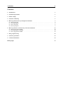
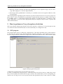
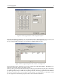
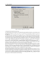
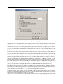
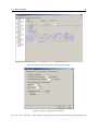
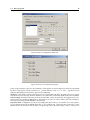
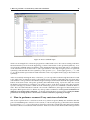
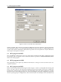
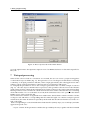
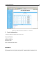
Missing 1.1
Short User Manual
Riccardo Gusmeroli and Claudia Dallera
Copyright 2004-2007 Riccardo Gusmeroli and Claudia Dallera.
All Rights Reserved
CONTENTS
II
Contents
1
Introduction
1
2
Installation procedure
1
3
Initial settings
1
4
Structure of Missing
1
5
How to perform an X-ray absorption calculation
5.1 RCN program . . . . . . . . . . . . . . . . . .
5.2 RCN2 program . . . . . . . . . . . . . . . . .
5.3 RCG program . . . . . . . . . . . . . . . . . .
5.4 Racer program . . . . . . . . . . . . . . . . . .
.
.
.
.
3
3
6
6
8
6
How to perform a resonant X-ray emission calculation
6.1 RCN program for RXES . . . . . . . . . . . . . . . . . . . . . . . . . . . . . . . . . . . . . .
6.2 RCN2 program for RXES . . . . . . . . . . . . . . . . . . . . . . . . . . . . . . . . . . . . . .
6.3 RCG program for RXES . . . . . . . . . . . . . . . . . . . . . . . . . . . . . . . . . . . . . .
13
14
14
14
7
Data postprocessing
15
8
Software generalities
17
9
Contact informations
18
Bibliography
.
.
.
.
.
.
.
.
.
.
.
.
.
.
.
.
.
.
.
.
.
.
.
.
.
.
.
.
.
.
.
.
.
.
.
.
.
.
.
.
.
.
.
.
.
.
.
.
.
.
.
.
.
.
.
.
.
.
.
.
.
.
.
.
.
.
.
.
.
.
.
.
.
.
.
.
.
.
.
.
.
.
.
.
.
.
.
.
.
.
.
.
.
.
.
.
.
.
.
.
18
1. Introduction
1
This document is an introductory guide to the use of the Personal Computer interface to the atomic
multiplet code based on Cowan’s programs. The name of the interface program is Missing: Multiplet
Inner-Shell Spectroscopy INterface GUI (please note that the code was formerly named RGAss and that
the screenshots contained in this manual were taken before the official name was given). The programs
that are accessed through the interface are listed here below, together with the name of the people who
developed the codes.
All programs listed above can be downloaded from the website
http://www.esrf.fr/UsersAndScience/Experiments/TBS/SciSoft/
where the present manual can also be found.
1
Introduction
In order to perform an Atomic Multiplet calculation several programs must be called subsequently. For
each of them we provide the printout of the screen with the explanation of the parameters that must be
the defined by the user. Many parameters do not need to be adjusted unless in very special cases. For
these parameters (that are not detailed in the present manual) we refer the reader to the original manual
by Robert Cowan, that can be downloaded from the site. Before starting with the use of the programs
some options can be defined through the menus. This is detailed in section 1. When the calculation is
finished the results can be exported to be viewed, as detailed in section ”How to look at results”.
2
Installation procedure
1. Obtain the package rgass.zip from the Web site http://www.esrf.fr/UsersAndScience/Experiments/TBS/SciSoft/
2. Unzip the package with your favourite unzip software to a folder called rgass (or any other name).
3. Go to folder rgass.
4. Double-click on Missing.exe
5. In Tools menu item click on the Install shell extensions command so that the Missing program is
automatically loaded when double-clicking on a .rgs file.
6. Again in Tools menu item click on the Re-install RCG command.
3
Initial settings
The files created through Missing are called Workspaces and have the extension .rgs. The initial page of
the program (Fig. 1) allows to create a new Workspace, to open an existing one, and to save the active
Wrokspace. Duplicating an existing workspace must be made from outside the program, infact the Save
as command is not active. The calls to the programs and their activation can be made from the Application
menu item as well as from the buttons located below. The Settings menu item gives access to settings
that affect the calculation and the export of the results, that can also be accessed from within the call to
each separate program. They will therefore be detailed in the section dedicated to the specific program.
General note: Missing allows to input the parameters through a user-friendly interface. However it also
allows to edit the input file, as in the origianl version. To do this check the Custom checkbox in the upper
left part of the screen that appears for each program call.
4
Structure of Missing
Missing is organized as a collection of chained calls to external scientific packages. In particular it is able
to manage the following applications:
4. Structure of Missing
2
Figure 1: Empty workspace.
• RCN [1] (by R. D. Cowan) calculates single-configuration radial wavefunctions Pnl (r) for a spherically symmetrized atom via homogeneous-differential-equation approximations to the HartreeFock method.
• RCN2 [1] (by R. D. Cowan) accepts radial wavefunctions (for one or more different configurations of one or more atoms or ions) from either RCN, and for each atom calculates various twoconfiguration radial integrals: overlap integrals hPnl |Pn0 l0 i, configuration-interaction Coulomb integrals Rk and spin-orbit integrals ζnln0 l0 , and radial electric-dipole and electric-quadrupole integrals.
• RCG [1] (by R. D. Cowan) computes the angular factor of various matrix elements involved in the
theory of atomic structure and spectra. It computes the XAS spectrum in spherical symmetry.
• RACER [2] (by B. T. Thole) calculates all the required quantities involved in point-group calculations. It computes the XAS spectrum in lower symmetry when the initial and final state are
characterized by one configuration only.
• TotalFluor (by B. T. Thole, H. Ogasawara, M. A. van Veenendaal, P. Ferriani, and C. M. Bertoni)
computes Hamiltonians and Transition matrices in lower symmetry. It computes the XAS spectrum in lower symmetry in cases of interacting configurations as well as Resonant Inelastic X-ray
Emission Spectra.
The sequence of the required calls, together with the provided options and data, are collected in a socalled workspace (which can be stored in a file with extension .rgs). When a workspace is runned, Missing
executes the external calls following three main steps:
1. Builds an input file on the base of user options and data (the user is also allowed to give the input
file directly if needed)
5. How to perform an X-ray absorption calculation
3
2. Runs the external executable in batch-mode grabbing the screen output messages, any error message and keeping trace of all the output data files
3. Rearranges all the grabbed data so that they are available to the user in separate windows of the
main program
After running all the required programs related to a specific calculation, the user can access a postprocess
phase where a series of useful plots are generated. In particular this option is available via the export
to an HTML archive: a web-ready hierarchical document is created with links to a summary of the
input/output data of each call and to high quality PDF plots and plot-ready raw files of spectra and
other useful functions.
5
How to perform an X-ray absorption calculation
This section details which steps must be followed to perform a calculation of X-ray absorption in the
case where the initial and the final state are characterized by one configuration only.
5.1
RCN program
The program RCN allows to define the configurations of the initial and final states of the transition.
To call it use the Add RCN call command from the Application menu bar, or the N button (see Fig. 2).
Use the Configure button to define the configurations of the initial and final state of the transition. Each
Figure 2: RCN program main panel.
configuration is called Card for obvious historical reasons.
To create a configuration card use the New... button from the screen shown in Fig. 3. Under the General
tab you must specify the element and can give a label to the element that you are investigating, for
instance Ni2+ (see Fig. 4). Do not worry about all the other parameters, they are fine as they are. Under
5.1
RCN program
4
Figure 3: RCN Configuration panel.
Figure 4: RCN General tab in the Configuration panel.
the Configuration tab you now specify the occupation numbers of all orbitals involved in the transition
and can give it a label (like 2p6 3d8, see Fig. 5).
When you have specified all configurations press OK. You can verify that the configurations that you
have created are possible initial and final states of a dipole transition by looking at their parity (either
the color of the arrow at the most left side, or the Parity column. The Show set arrangment button tells
you whether the configurations have the same ionization state.
To modify a configuration card click on it and use the Configuration button. You can change the order of
the created configurations by using the up and down arrow buttons.
Finally, the Parameters button gives access to a large number of parameters that determine the accuracy
of the calculation. They give origin to all the numbers that apear in the first row of the input. Some of
5.1
RCN program
5
Figure 5: RCN Configuration tab in the Configuration panel.
them are self-explanatory, many are not. You should not need to change them. In case you really wish
to know their meaning and effect you are welcome to refer to Cowan’s original manuals.
Now you can press the Done button. You should see something similar to Fig. 6.
Figure 6: RCN Configuration panel after creation of configuration.
One more button, that is present in most of the program calls is the HTML button. This button is to
definy the format and content of the HTML output.
When you have performed all the detailed steps run the program, either through the Run command in
the Applications menu, or through the button with the exclamation mark. It is not mandatory to run each
program separately and you could run everything at the end, when all programs have been defined.
However, it is better if you do it at each step: in fact by doing so you will be able to see the input created
by each program for the following program, and to follow better the instructions.
5.2
5.2
RCN2 program
6
RCN2 program
The program RCN2 computes the average energies, the radial integrals and the spin-orbit parameters
of the electornic configurations defined in RCN. To call the program use the Add RCN2 call command
from the Application menu bar, or the 2 button (see Fig. 7). In this program you can set some parameters
Figure 7: RCN2 program main panel.
that influence the calculation performe in the subsequent steps: this is done through the The program
RCN allows to define the configurations of the initial and final states of the transition. To call it use the
Configure... button.
The General tab (Fig. 8) defines whether the radial integrals are multiplied by the overlap integrals and
whether the inetgrals needed for the computation of an electric quadrupole transition should be calculated.
The Numeric Parameters tab (Fig. 9)is particularly important. It defines the factor for rescaling the
Slater integral values with respect to their atomic value in order to simulate the effect of the intraatomic correlation not accounted for in the HartreeFock approximation. F k (li , lj ), F k (li , li ), Gk (li , lj )
and Rk (li , lj , li0 , lj0 ) are the Slater integrals involving different shells. ζi is the spin-orbit parameter. The
”normally” used values of the rescaling factors are 0.8 for the Slater integrals and 1 for the spin-orbit
factor.
Note that the order in which these parameters are listed is used to identify them as they appear in the
input of RCG (see following section).
The Output tab (Fig. 10) does not require to be modified.
5.3 RCG program
The program RCG receives as input the output from program RCN2 and computes the eigenvectors and
eigenvalues of the specified configurations. If the calculation is performed in spherical symmetry (we
explain later how to defien the symmetry) then it will also compute the absorption spectrum. Otherwise
5.3
RCG program
7
Figure 8: RCN2 Configuration General tab.
it will produce the input for the next step.
To call the program use the Add RCG call command from the Application menu bar, or the G button. The
main panel will appear as in Fig. 11 if you have not run the previous programs. Otherwise it will look
as in Fig. 12.
The input that appears in the panel is the output of RCN2. As anticipated in the description of the RCN2
parameters, the values listed after each configuration are the average energy, the Slater integrals and the
spin-orbit parameter. They are identified by the last digit, that corresponds to the order in which they
are listed in the Numeric Parameters tab of the Configuration of RCN2: vaules ending with 0 indicate the
average energy, ending with 1 indicate the Slater parameter of type F k (li , lj ), with 2 the Slater parameter
F k (li , li ), with 3 the Slater parameter Gk (li , lj ) and with 4 the Slater parameter Rk (li , lj , li0 , lj0 ) (that is
used only in those cases where interaction among different configuration in the same state is used).
The Configure... button has many tabs, of which we address only the General and the RME ones. The
Printout 1, Printout 2 and Printout 3 tabs do not need to be modified, and the Rearrange tab will be
detailed later when describing how an X-ray emission calculation is performed.
The General (shown in Fig. 13) is to be used in cases that are slightly more sophisticated than the example
that we are giving here, i.e. in the cases where interaction among different configurations must be
taken into account. So, if the initial state (referred to as First parity/lower level or the final state Second
parity/upper level) is made up by more than one of the configurations listed in RCN, this must be declared
in the Transitions to be included box. We do not detail here the other boxes, which are not of broad use,
apart from the Coupling box, that allows to select between LS and JJ coupling.
The RME tab (RME stands for Reduced Matrix Elements) is extremely important and is needed in all cases
where the calculations are performed in non-spherical symmetry. This tab is shown in Fig. 14. The
terms that must be added to the spherical hamiltonian are specified here in form of Operators: the Shell
operator allows to specify the particular symmetry (cubic Oh, tetrahedral C4h, ...) of the system. The
Spin operator is required to specify the presence of an exchange-split field. The procedure to include
those operators in the calculation is the following:
5.4
Racer program
8
Figure 9: RCN2 Configuration Numeric Parameters panel.
Choose the operator through the Add... button
Check the box corresponding to the parity (i.e. the initial or final state, or both) and orbital on which the
operator should act. The order of the orbitals corresponds to the one listed in the input of RCN.
You will need to modify the numbers in the following lines of the panel in some special cases: the
minimum and maximum values of J (for Crystal Field matrix elements calculation) are 4 most of the time
but might be 2 and 6 in some cases (as the one of the present example). We will give some hint about
this point in the section 5.4. The Pole values of the Interaction matrix elements calculation are always 1 for
transitions governed by electric dipole operators, they would be 2 for quadrupolar transitions. Finally,
the number after Number of interacting shells: indicates that only for the specified number of shells in
each state the Slater integrals and spin-orbit parameters will be included in the calculation. Further
shells will be considered to be ’continuum’ or ’ligand’ shells.
If some operators have been chosen in the RME tab, then the calculation must continue with the Racer
program.
In the case of a system that is well described in spherical symmetry, the calculation ends when running
RCG. After this the spectra can be generated and viewed through the button located to the right of the
exclamation mark (or through the Export as HTML command in the File menu item) as detailed in 7. The
parameters that define the generated spectrum must be defined through the HTML button on the main
screen.
if only the HTML parameters are changed, there is no need to re-run the calculation, exporting is
enough. The same holds for the Racer program.
5.4
Racer program
The Racer program comes after the RCG program. The call can be added only when Operators have been
selected in RCG, as explained in the previous section (you will get an error otherwise). The input of
Racer is loaded through the Load Standard File... button (Fig. 15). The button gives access to a number
of inputs for calculating the spectra in different symmetries. Each item of the Load Racer Standard File
5.4
Racer program
9
Figure 10: RCN2 Configuration Output panel.
input specifies the starting symmetry (always spherical O3) and the desired symmetry for the system.
The available inputs are for calculations in the Oh, O2 and C4h symmetry. Note that for an absorption
calculation you have to select among the options without TFluor: these are the input files for emission
calculations and will be explained later.
We give some details about the structure of the input shown in Fig. 16 in order to enable the user of the
programs to modify them.
The input always starts with Y. The next line contains the name of the routine that is called (Butler for
absorption calculation and Racer for resonant inelastic X-ray emission calculations. The labels that follow give the chain of the symmetries (with their parities) through which the calculations goes from the
spherical to the final symmetry. For more information on how to construct these chains you can refer to
Chapter 12 in the book by P.H. Butler in Ref. [2]. The available inputs should to the job for most cases.
The following blocks describe the structure of the Hamiltonian for the ground and excited state. With
reference to FigureXXX, the Hamiltonian ACTOR, having symmetry 0+ in Butler’s notation, is composed by three OPERators (HAMILTONIAN, SHELL2 and SPIN2), that refer respectively to the spherical
part of the Hamiltonian, to the Crystal Field part, and to the magnetic exchange interaction part. Note
that the operators SHELL and SPIN end with a number: this number indicates the shell on which the
operator acts and must correspond to the number specified in the RME tab of the input of RCG.
After each operator comes the keyword BRANCH followed by a list of symbols intercalated by > numbers. These symbols express the symmetry (in Butler’s group notation) through which the system is
transformed from the initial spherical to the final desired symmetry (tetrhaedral C4H in the present example). Numbers not followed by a + or − sign indicate multeplicity (0 means 1).
The last number of each BRANCH line indicates the strength of the operator. The number that ends
the BRANCH lines of the SHELL2 operators is related to the Crystal Field parameters 10Dq, Ds and Dt.
These are among the most important parameters you want to include in the calculation, so they deserve
some precise practical information on how to use them:
in the case of C4H calculation like the present one, 10Dq, Ds and Dt are specified separately. The num-
5.4
Racer program
10
Figure 11: RCG program main panel.
bers that appear in the input of Racer are X 400 , X 420 and X 220 (this is easily remembered by looking at
the BRANCH lines (containing respectively 4+ 0+ 0+, 4+ 2+ 0+, 2+ 2+ 0+). It will be useful to recall here
the relations between the 10Dq, Ds, Dt and the X 400 , X 420 and X 220 :
X 400
X 420
X 220
√
= 30 ×√(6Dq − 72 Dt)
7
42 × (Dt)
= −√
2 ×
= − 70 × (Ds)
In case of cubic Oh symmetry only the 10Dq parameter needs to be specified. In this case the relationship between 10Dq and X 400 is:
X 400
=
√
30 × (6Dq)
In practice, in
√ the case of Oh symmetry, in order to specify the value of 10Dq in eV , you must multiply
it by 6/10 × 30, i.e. by 3.286335345. In the input file of the example, the value given for X 400 indicates
that 10Dq was 1 eV (Ds and Dt are 0 in the example).
The number that ends the BRANCH lines of the SPIN2 operators gives the value (in eV ) of the magnetic
exchange interaction.
Similar blocks are repeated for the initial ground and the excited final state.
The last block in the input file describes the transition, in particular the symmetry of the operators that
5.4
Racer program
11
Figure 12: RCG program main panel completed with input.
Figure 13: RCG Configuration General tab.
give rise to the absorption. The symbols following the keyword ACTOR indicate the symmetry and
5.4
Racer program
12
Figure 14: RCG Configuration RME tab.
Figure 15: Racer Load Standard File input.
parity of the transition operator: the symmetry of the light in an electric dipolar transition is described
by three components, usually referred to as q, which take the value 1, 0, −1. The − sign that follows
indicates that the dipolar transition operator has odd parity.
Warning: if the input contains names that are not recognized by the Racer program, the Screen Output
will show the error message PIPPPO (Italian for Foo): this tells you that the input needs to be modified.
Side warning: the names following ACTOR are labels that can be chosen freely. We suggest however to
make as little as possibile modifications to the input we provide, in order to reduce the risk of mistakes.
The names following OPER cannot be chosen freely.
Important hint: As might be clear by now, building the input of Racer, for instance for a new symmetry, not listed among the standard input files, is not without risk. Especially the construction of the
BRANCH lines from scratch can be tricky. Of great help can be the Tape Output of Racer, some part of
6. How to perform a resonant X-ray emission calculation
13
Figure 16: Racer standard input.
which are meaningful also when the program has ended with errors: the section starting with REPRESENTATIONS (not far from the beginning), contains all branches for the specified symmetry. As is
clear from the standard inputs, branchings of the HAMILTONIAN actor must end with 0+, branchings
of the MULTIPOLE actors start with 1− (the representation of the dipolar light operator in spherical
symmetry) and end with the same symmetry as the operator (i.e. 1+ for the light operator q = 1+ and
so on). The branches representation listed in that file can be very helpful when trying to deal with a new
symmetry.
After successufully running the Racer calculation, you can export the results through the button located
to the right of the exclamation mark (or through the Export as HTML command in the File menu item)
as detailed in 7. The parameters that define the generated spectrum must be defined through the HTML
button on the main screen. The panel opened by the HTML button (Fig. 17) has two tabs: the General
tab defines self-explanatory parameters very similar to those of the RCG program. The often forgotten
Operators tab (Fig. 18) allows to define how the elementary spectra are combined to build the final results. The Load C4H-LZR button loads the 7 most used combinations, that appear in the bottom part of
the panel. Blank spectra allow to define any other possible combination. If no spectral combination is
defined, no spectrum will be computed. As already said in the RCG program section, if only the HTML
parameters are changed, there is no need to re-run the calculation, exporting is enough.
6
How to perform a resonant X-ray emission calculation
This section explains how to calculate resonant X-ray emission spectra (RXES). We underline that this
part is for resonant spectra: in fact for non-resonant, i.e. fluorescent spectra, good results can be obtained
by performing a reversed X-ray absorption calculation, where the excited state is the initial state and the
final state is the less-excited state in the transition. In the resonant case the Kramers-Heisenberg formula
6.1
RCN program for RXES
14
Figure 17: Racer General tab in the HTML button.
must be included. This is done by performing an additional step in the calculation. We here explain the
whole program sequence: in fact all programs detailed before must be used in a sligthly different way,
as three states (initial, intermediate, final) must be specified. We will explain here only the differences
with respect to absorption calculation.
6.1
RCN program for RXES
The only difference with respect to the case of absorption calculation is that three configurations must
be specified. Take care that the order in which they must be specified is: Initial, Intermediate, Final.
This is all for this program.
6.2
RCN2 program for RXES
This program does not require any additional information to what give in the section devoted to absorption calculation.
6.3
RCG program for RXES
In RCG some more parameters must be given in the Configure... button: as anticipated, the Rearrange tab
plays a role here: the role of the declared configurations must be specified. In the given example the
ground state contains the first configuration, the intermediate state is the third configuration, and the
final state is the second configuration (in case of state with multiple, interacting configurations, the panel
allows to specify groups of configurations). The lower block (the one referring to TFluor calculations only
7. Data postprocessing
15
Figure 18: Racer Operators tab in the HTML button.
gives the right format to the input RCG input in view of an RXES calculation: in fact in the input file for
RCG, the
7
Data postprocessing
When all the calls involved in a calculation are executed, the user can access a postprocessing phase
via the button Export as HTML (Fig. 19). This generates a sort of workspace documentation containing
a summary of all input parameters and data, all the output generated by the called applications and a
number of plots of physical quantities of interest such as wavefunctions and spectra.
To exemplify the procedure we choose the workspace generated in the N iO XAS example of section 5
(Fig. 19). Once the Export as HTML button is pressed, a dialog window asks the user for the filename
(with extension .html) of the main documentation file. In this context we choose the name NiOXAS.html:
Missing will then create an index file called NiOXAS.html and a folder called NiOXAS files containing
all the indexed files. As soon as the data are stored, the documentation tree is also opened in the default
HTML viewer of the system (Fig. 20).
The documentation window is organized in two tiled frames: the left frame contains an index of all the
workspace calls and links to corresponding data files while the right one contains workspace general
informations (this latter document is replaced by the desired data document when the user clicks on a
link on the right).
Items corresponding to each call include three fixed data files (namely Input, Screen and Tape) and other
application-specific ones:
• Input: contains all the parameters and the data provided by the user, together with the formatted
7. Data postprocessing
16
Figure 19: Workspace at the end of a run command. The red circle highlights the Export as HTML button.
input file generated.
• Screen: shows the messages printed on the screen during program execution.
• Tape: contains all the human-readable genrated tapes
• Results (where applicable): links to all the post-processed data such as wavefunctions and spectra.
In our case we are interested to the absorption spectra in C4H symmetry (which in turn was generated by
the call to Racer labelled ”(03)”). To that aim we click on the Results link under the section ”(03) RACER”
of the left frame, obtaining the view in Fig. 21. A brief description of the resulting page follows:
• A frame in the top section tells the symmetry of interest (C4H in the example) and the transformation chain used to reach it (O3 → OH → D4H → C4H )
• Under the label Triads a list of the transition matrices parsed can be found
• In the Spectra frame the user can access the spectral data of interest. In particular:
1. Near the words Lines selected the number of spectral lines selected on the base of user-provided
parameters can be found. The word selected points to a text-based file with a list of all such
lines.
2. The statement Spectra plots and tables introduces the available plots. The word plots points to
a high-quality PDF file containing all the generated plots in a print-ready fashion. Each plot
can also be retrieved in a text-based data file using the following links.
8. Software generalities
17
Figure 20: Index file of the documentation tree opened in the default HTML viewer.
8 Software generalities
Missing 1.1
Copyright 2001-2004 Riccardo Gusmeroli.
All rights reserved.
The software is a user-friendly PC interface to the Atomic Multiplet Code written by R.D.Cowan
(LANL) with extensions by B.T.Thole and others. Porting from the original code to the PC-compatible
version is intrinsically prone to the arising of bugs. Many of them have been found and removed by
the author but others might still be present. In case of results that are suspicious because undoubtedly
contrasting physical expectations, please contact the author enclosing the indicted workspace (see 9 for
contact informations).
The right to use the software free of charge is granted to scientific institution provided a reference to
the code and its author is included in any publication it contributes to. Any commercial use is instead
prohibited without explicit authorization by the author.
The software is provided ”as is”, without warranty of any kind, express or implied, including but not
limited to the warranties of merchantability, fitness for a particular purpose and noninfringement. In
no event shall the author be liable for any claim, damages or other liability, whether in an action of contract, tort or otherwise, arising from, out of or in connection with Missing or the use or other dealings in
Missing.
9. Contact informations
Figure 21: Postprocessed results of the Racer C4H calculation.
9
Contact informations
Comments, suggestions and bug-reports can be sent to:
Prof. Claudia Dallera
Dipartimento di Fisica
Politecnico di Milano
Piazza L. Da Vinci, 32
20133 Milano (MI)
Email: [email protected]
References
[1] R. D. Cowan, The Theory of Atomic Structure and Spectra. University of California Press, 1981.
[2] P. H. Butler, Point Group Symmetry and Applications - Methods and Tables. Plenum Press, 1981.
18