Download Functional programming using Caml Light

Functional programming
using Caml Light
Michel Mauny
January 1995
Contents
1 Introduction
5
I
7
Functional programming
2 Functional languages
9
2.1 History of functional languages . . . . . . . . . . . . . . . . . . . . . . . . . . . . . . 10
2.2 The ML family . . . . . . . . . . . . . . . . . . . . . . . . . . . . . . . . . . . . . . . 10
2.3 The Miranda family . . . . . . . . . . . . . . . . . . . . . . . . . . . . . . . . . . . . 11
3 Basic concepts
3.1 Toplevel loop . . . . . . . . . .
3.2 Evaluation: from expressions to
3.3 Types . . . . . . . . . . . . . .
3.4 Functions . . . . . . . . . . . .
3.5 Definitions . . . . . . . . . . . .
3.6 Partial applications . . . . . . .
4 Basic types
4.1 Numbers . . . . . . . . . . . . .
4.2 Boolean values . . . . . . . . .
4.3 Strings and characters . . . . .
4.4 Tuples . . . . . . . . . . . . . .
4.5 Patterns and pattern-matching
4.6 Functions . . . . . . . . . . . .
. . . .
values
. . . .
. . . .
. . . .
. . . .
.
.
.
.
.
.
.
.
.
.
.
.
.
.
.
.
.
.
.
.
.
.
.
.
.
.
.
.
.
.
.
.
.
.
.
.
.
.
.
.
.
.
.
.
.
.
.
.
.
.
.
.
.
.
.
.
.
.
.
.
.
.
.
.
.
.
.
.
.
.
.
.
.
.
.
.
.
.
.
.
.
.
.
.
.
.
.
.
.
.
.
.
.
.
.
.
.
.
.
.
.
.
.
.
.
.
.
.
.
.
.
.
.
.
.
.
.
.
.
.
.
.
.
.
.
.
.
.
.
.
.
.
.
.
.
.
.
.
.
.
.
.
.
.
.
.
.
.
.
.
.
.
.
.
.
.
.
.
.
.
.
.
.
.
.
.
.
.
.
.
.
.
.
.
.
.
.
.
.
.
.
.
.
.
.
.
.
.
.
.
.
.
.
.
.
.
.
.
.
.
.
.
.
.
.
.
.
.
.
.
.
.
.
.
.
.
.
.
.
.
.
.
.
.
.
.
.
.
.
.
.
.
.
.
.
.
.
.
.
.
.
.
.
.
.
.
.
.
.
.
.
.
.
.
.
.
.
.
.
.
.
.
.
.
.
.
.
.
.
.
.
.
.
.
.
.
.
.
.
.
.
.
.
.
.
.
.
.
.
.
.
.
.
.
.
.
.
.
.
.
.
.
.
.
.
.
.
.
.
.
.
.
.
.
.
.
.
.
.
.
.
.
.
.
.
.
.
.
.
.
13
13
14
15
17
17
19
.
.
.
.
.
.
21
21
24
26
27
28
30
5 Lists
33
5.1 Building lists . . . . . . . . . . . . . . . . . . . . . . . . . . . . . . . . . . . . . . . . 33
5.2 Extracting elements from lists: pattern-matching . . . . . . . . . . . . . . . . . . . . 34
5.3 Functions over lists . . . . . . . . . . . . . . . . . . . . . . . . . . . . . . . . . . . . . 35
6 User-defined types
37
6.1 Product types . . . . . . . . . . . . . . . . . . . . . . . . . . . . . . . . . . . . . . . . 37
6.2 Sum types . . . . . . . . . . . . . . . . . . . . . . . . . . . . . . . . . . . . . . . . . . 39
6.3 Summary . . . . . . . . . . . . . . . . . . . . . . . . . . . . . . . . . . . . . . . . . . 45
1
2
II
CONTENTS
Caml Light specifics
47
7 Mutable data structures
7.1 User-defined mutable data structures . . . .
7.2 The ref type . . . . . . . . . . . . . . . . .
7.3 Arrays . . . . . . . . . . . . . . . . . . . . .
7.4 Loops: while and for . . . . . . . . . . . .
7.5 Polymorphism and mutable data structures
.
.
.
.
.
.
.
.
.
.
.
.
.
.
.
.
.
.
.
.
.
.
.
.
.
.
.
.
.
.
.
.
.
.
.
.
.
.
.
.
.
.
.
.
.
.
.
.
.
.
.
.
.
.
.
.
.
.
.
.
.
.
.
.
.
.
.
.
.
.
.
.
.
.
.
.
.
.
.
.
.
.
.
.
.
.
.
.
.
.
.
.
.
.
.
.
.
.
.
.
.
.
.
.
.
.
.
.
.
.
.
.
.
.
.
49
49
50
51
52
54
8 Escaping from computations: exceptions
8.1 Exceptions . . . . . . . . . . . . . . . . .
8.2 Raising an exception . . . . . . . . . . . .
8.3 Trapping exceptions . . . . . . . . . . . .
8.4 Polymorphism and exceptions . . . . . . .
.
.
.
.
.
.
.
.
.
.
.
.
.
.
.
.
.
.
.
.
.
.
.
.
.
.
.
.
.
.
.
.
.
.
.
.
.
.
.
.
.
.
.
.
.
.
.
.
.
.
.
.
.
.
.
.
.
.
.
.
.
.
.
.
.
.
.
.
.
.
.
.
.
.
.
.
.
.
.
.
.
.
.
.
.
.
.
.
.
.
.
.
.
.
.
.
55
55
56
57
58
9 Basic input/output
9.1 Printable types .
9.2 Output . . . . .
9.3 Input . . . . . . .
9.4 Channels on files
.
.
.
.
.
.
.
.
.
.
.
.
.
.
.
.
.
.
.
.
.
.
.
.
.
.
.
.
.
.
.
.
.
.
.
.
.
.
.
.
.
.
.
.
.
.
.
.
.
.
.
.
.
.
.
.
.
.
.
.
.
.
.
.
.
.
.
.
.
.
.
.
.
.
.
.
.
.
.
.
.
.
.
.
.
.
.
.
.
.
.
.
.
.
.
.
.
.
.
.
.
.
.
.
.
.
.
.
.
.
.
.
.
.
.
.
.
.
.
.
.
.
.
.
.
.
.
.
59
59
61
62
62
10 Streams and parsers
10.1 Streams . . . . . . . . . . . .
10.2 Stream matching and parsers
10.3 Parameterized parsers . . . .
10.4 Further reading . . . . . . . .
.
.
.
.
.
.
.
.
.
.
.
.
.
.
.
.
.
.
.
.
.
.
.
.
.
.
.
.
.
.
.
.
.
.
.
.
.
.
.
.
.
.
.
.
.
.
.
.
.
.
.
.
.
.
.
.
.
.
.
.
.
.
.
.
.
.
.
.
.
.
.
.
.
.
.
.
.
.
.
.
.
.
.
.
.
.
.
.
.
.
.
.
.
.
.
.
.
.
.
.
.
.
.
.
.
.
.
.
.
.
.
.
.
.
.
.
.
.
.
.
.
.
.
.
65
65
67
69
76
.
.
.
.
.
.
.
.
.
.
.
.
.
.
.
.
.
.
.
.
.
.
.
.
11 Standalone programs and separate compilation
79
11.1 Standalone programs . . . . . . . . . . . . . . . . . . . . . . . . . . . . . . . . . . . . 79
11.2 Programs in several files . . . . . . . . . . . . . . . . . . . . . . . . . . . . . . . . . . 80
11.3 Abstraction . . . . . . . . . . . . . . . . . . . . . . . . . . . . . . . . . . . . . . . . . 82
III
A complete example
85
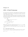
12 ASL: A Small Language
87
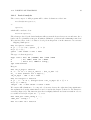
12.1 ASL abstract syntax trees . . . . . . . . . . . . . . . . . . . . . . . . . . . . . . . . . 87
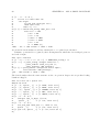
12.2 Parsing ASL programs . . . . . . . . . . . . . . . . . . . . . . . . . . . . . . . . . . . 88
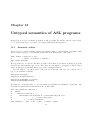
13 Untyped semantics of
13.1 Semantic values . .
13.2 Semantic functions
13.3 Examples . . . . .
ASL programs
. . . . . . . . . . . . . . . . . . . . . . . . . . . . . . . . . . . . .
. . . . . . . . . . . . . . . . . . . . . . . . . . . . . . . . . . . . .
. . . . . . . . . . . . . . . . . . . . . . . . . . . . . . . . . . . . .
93
93
94
95
14 Encoding recursion
97
14.1 Fixpoint combinators . . . . . . . . . . . . . . . . . . . . . . . . . . . . . . . . . . . . 97
14.2 Recursion as a primitive construct . . . . . . . . . . . . . . . . . . . . . . . . . . . . 98
CONTENTS
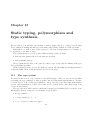
15 Static typing, polymorphism and type
15.1 The type system . . . . . . . . . . . .
15.2 The algorithm . . . . . . . . . . . . . .
15.3 The ASL type-synthesizer . . . . . . .
3
synthesis
99
. . . . . . . . . . . . . . . . . . . . . . . . . . 99
. . . . . . . . . . . . . . . . . . . . . . . . . . 103
. . . . . . . . . . . . . . . . . . . . . . . . . . 105
16 Compiling ASL to an abstract machine code
16.1 The Abstract Machine . . . . . . . . . . . . . . . . . . . . . . . . . . . . . . . . . .
16.2 Compiling ASL programs into CAM code . . . . . . . . . . . . . . . . . . . . . . .
16.3 Execution of CAM code . . . . . . . . . . . . . . . . . . . . . . . . . . . . . . . . .
115
. 115
. 118
. 120
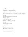
17 Answers to exercises
123
18 Conclusions and further reading
135
4
CONTENTS
Chapter 1
Introduction
This document is a tutorial introduction to functional programming, and, more precisely, to the
usage of Caml Light. It has been used to teach Caml Light1 in different universities and is intended
for beginners. It contains numerous examples and exercises, and absolute beginners should read it
while sitting in front of a Caml Light toplevel loop, testing examples and variations by themselves.
After generalities about functional programming, some features specific to Caml Light are
described. ML type synthesis and a simple execution model are presented in a complete example
of prototyping a subset of ML.
Part I (chapters 2–6) may be skipped by users familiar with ML. Users with experience in
functional programming, but unfamiliar with the ML dialects may skip the very first chapters and
start at chapter 6, learning the Caml Light syntax from the examples. Part I starts with some
intuition about functions and types and gives an overview of ML and other functional languages
(chapter 2). Chapter 3 outlines the interaction with the Caml Light toplevel loop and its basic
objects. Basic types and some of their associated primitives are presented in chapter 4. Lists
(chapter 5) and user-defined types (chapter 6) are structured data allowing for the representation
of complex objects and their easy creation and destructuration.
While concepts presented in part I are common (under one form or another) to many functional
languages, part B (chapters 7–11) is dedicated to features specific to Caml Light: mutable data
structures (chapter 7), exception handling (chapter 8), input/output (chapter 9) and streams and
parsers (chapter 10) show a more imperative side of the language. Standalone programs and
separate compilation (chapter 11) allow for modular programming and the creation of standalone
applications. Concise examples of Caml Light features are to be found in this part.
Part C (chapters 12–16) is meant for already experienced Caml Light users willing to know more
about how the Caml Light compiler synthesizes the types of expression and how compilation and
evaluation proceeds. Some knowledge about first-order unification is assumed. The presentation
is rather informal, and is sometimes terse (specially in the chapter about type synthesis). We
prototype a small and simple functional language (called ASL): we give the complete prototype
implementation, from the ASL parser to the symbolic execution of code. Lexing and parsing of ASL
programs are presented in chapter 12, providing realistic usages of streams and parsers. Chapter
13 presents an untyped call-by-value semantics of ASL programs through the definition of an ASL
interpreter. The encoding of recursion in untyped ASL is presented in chapter 14, showing the
1
The “Caml Strong” version of these notes is available as an INRIA technical report [26].
5
6
CHAPTER 1. INTRODUCTION
expressive power of the language. The type synthesis of functional programs is demonstrated in
chapter 15, using destructive unification (on first-order terms representing types) as a central tool.
Chapter 16 introduces the Categorical Abstract Machine: a simple execution model for call-byvalue functional programs. Although the Caml Light execution model is different from the one
presented here, an intuition about the simple compilation of functional languages can be found in
this chapter.
Warning: The programs and remarks (especially contained in parts B and C) might not be
valid in Caml Light versions different from 0.7.
Part I
Functional programming
7
Chapter 2
Functional languages
Programming languages are said to be functional when the basic way of structuring programs is
the notion of function and their essential control structure is function application. For example,
the Lisp language [22], and more precisely its modern successor Scheme [31, 1], has been called
functional because it possesses these two properties.
However, we want the programming notion of function to be as close as possible to the usual
mathematical notion of function. In mathematics, functions are “first-class” objects: they can be
arbitrarily manipulated. For example, they can be composed, and the composition function is itself
a function.
In mathematics, one would present the successor function in the following way:
successor : N −→ N
n 7−→ n + 1
The functional composition could be presented as:
◦ : (A ⇒ B) × (C ⇒ A) −→ (C ⇒ B)
(f, g) 7−→ (x 7−→ f (g x))
where (A ⇒ B) denotes the space of functions from A to B.
We remark here the importance of:
1. the notion of type; a mathematical function always possesses a domain and a codomain. They
will correspond to the programming notion of type.
2. lexical binding: when we wrote the mathematical definition of successor, we have assumed
that the addition function + had been previously defined, mapping a pair of natural numbers
to a natural number; the meaning of the successor function is defined using the meaning of
the addition: whatever + denotes in the future, this successor function will remain the same.
3. the notion of functional abstraction, allowing to express the behavior of f ◦ g as
(x 7−→ f (g x)), i.e. the function which, when given some x, returns f (g x).
ML dialects (cf. below) respect these notions. But they also allow non-functional programming
styles, and, in this sense, they are functional but not purely functional.
9
10
CHAPTER 2. FUNCTIONAL LANGUAGES
2.1
History of functional languages
Some historical points:
• 1930: Alonzo Church developed the λ-calculus [6] as an attempt to provide a basis for mathematics. The λ-calculus is a formal theory for functionality. The three basic constructs of
the λ-calculus are:
– variable names (e.g. x, y,. . . );
– application (M N if M and M are terms);
– functional abstraction (λx.M ).
Terms of the λ-calculus represent functions. The pure λ-calculus has been proved inconsistent as a logical theory. Some type systems have been added to it in order to remedy this
inconsistency.
• 1958: Mac Carthy invented Lisp [22] whose programs have some similarities with terms of
the λ-calculus. Lisp dialects have been recently evolving in order to be closer to modern
functional languages (Scheme), but they still do not possess a type system.
• 1965: P. Landin proposed the ISWIM [18] language (for “If You See What I Mean”), which
is the precursor of languages of the ML family.
• 1978: J. Backus introduced FP: a language of combinators [3] and a framework in which it is
possible to reason about programs. The main particularity of FP programs is that they have
no variable names.
• 1978: R. Milner proposes a language called ML [11], intended to be the metalanguage of the
LCF proof assistant (i.e. the language used to program the search of proofs). This language
is inspired by ISWIM (close to λ-calculus) and possesses an original type system.
• 1985: D. Turner proposed the Miranda [36] programming language, which uses Milner’s type
system but where programs are submitted to lazy evaluation.
Currently, the two main families of functional languages are the ML and the Miranda families.
2.2
The ML family
ML languages are based on a sugared1 version of λ-calculus. Their evaluation regime is call-byvalue (i.e. the argument is evaluated before being passed to a function), and they use Milner’s type
system.
The LCF proof system appeared in 1972 at Stanford (Stanford LCF). It has been further
developed at Cambridge (Cambridge LCF) where the ML language was added to it.
From 1981 to 1986, a version of ML and its compiler was developed in a collaboration between
INRIA and Cambridge by G. Cousineau, G. Huet and L. Paulson.
1
i.e. with a more user-friendly syntax.
2.3. THE MIRANDA FAMILY
11
In 1981, L. Cardelli implemented a version of ML whose compiler generated native machine
code.
In 1984, a committee of researchers from the universities of Edinburgh and Cambridge, Bell
Laboratories and INRIA, headed by R. Milner worked on a new extended language called Standard
ML [28]. This core language was completed by a module facility designed by D. MacQueen [23].
Since 1984, the Caml language has been under design in a collaboration between INRIA and
LIENS2 ). Its first release appeared in 1987. The main implementors of Caml were Ascánder Suárez,
Pierre Weis and Michel Mauny.
In 1989 appeared Standard ML of New-Jersey, developed by Andrew Appel (Princeton University) and David MacQueen (Bell Laboratories).
Caml Light is a smaller, more portable implementation of the core Caml language, developed
by Xavier Leroy since 1990.
2.3
The Miranda family
All languages in this family use lazy evaluation (i.e. the argument of a function is evaluated if and
when the function needs its value—arguments are passed unevaluated to functions). They also use
Milner’s type system.
Languages belonging to the Miranda family find their origin in the SASL language [34] (1976)
developed by D. Turner. SASL and its successors (KRC [35] 1981, Miranda [36] 1985 and Haskell
[15] 1990) use sets of mutually recursive equations as programs. These equations are written in a
script (collection of declarations) and the user may evaluate expressions using values defined in this
script. LML (Lazy ML) has been developed in Göteborg (Sweeden); its syntax is close to ML’s
syntax and it uses a fast execution model: the G-machine [16].
2
Laboratoire d’Informatique de l’Ecole Normale Supérieure, 45 Rue d’Ulm, 75005 Paris
12
CHAPTER 2. FUNCTIONAL LANGUAGES
Chapter 3
Basic concepts
We examine in this chapter some fundamental concepts which we will use and study in the following
chapters. Some of them are specific to the interface with the Caml language (toplevel, global
definitions) while others are applicable to any functional language.
3.1
Toplevel loop
The first contact with Caml is through its interactive aspect1 . When running Caml on a computer,
we enter a toplevel loop where Caml waits for input from the user, and then gives a response to
what has been entered.
The beginning of a Caml Light session looks like this (assuming $ is the shell prompt on the
host machine):
$camllight
>
Caml Light version 0.6
#
On the PC version, the command is called caml.
The “#” character is Caml’s prompt. When this character appears at the beginning of a line in
an actual Caml Light session, the toplevel loop is waiting for a new toplevel phrase to be entered.
Throughout this document, the phrases starting by the # character represent legal input to
Caml. Since this document has been pre-processed by Caml Light and these lines have been
effectively given as input to a Caml Light process, the reader may reproduce by him/herself the
session contained in each chapter (each chapter of the first two parts contains a different session, the
third part is a single session). Lines starting with the “>” character are Caml Light error messages.
Lines starting by another character are either Caml responses or (possibly) illegal input. The input
is printed in typewriter font (like this), and output is written using slanted typewriter font (like
that).
Important: Of course, when developing non-trivial programs, it is preferable to edit programs
in files and then to include the files in the toplevel, instead of entering the programs directly.
1
Caml Light implementations also possess a batch compiler usable to compile files and produce standalone applications; this will be discussed in chapter 11.
13
14
CHAPTER 3. BASIC CONCEPTS
Furthermore, when debugging, it is very useful to trace some functions, to see with what arguments
they are called, and what result they return. See the reference manual [21] for a description of
these facilities.
3.2
Evaluation: from expressions to values
Let us enter an arithmetic expression and see what is Caml’s response:
#1+2;;
- : int = 3
The expression “1+2” has been entered, followed by “;;” which represents the end of the current
toplevel phrase. When encountering “;;”, Caml enters the type-checking (more precisely type
synthesis) phase, and prints the inferred type for the expression. Then, it compiles code for the
expression, executes it and, finally, prints the result.
In the previous example, the result of evaluation is printed as “3” and the type is “int”: the
type of integers.
The process of evaluation of a Caml expression can be seen as transforming this expression
until no further transformation is allowed. These transformations must preserve semantics. For
example, if the expression “1+2” has the mathematical object 3 as semantics, then the result “3”
must have the same semantics. The different phases of the Caml evaluation process are:
• parsing (checking the syntactic legality of input);
• type synthesis;
• compiling;
• loading;
• executing;
• printing the result of execution.
Let us consider another example: the application of the successor function to 2+3. The expression
(function x -> x+1) should be read as “the function that, given x, returns x+1”. The juxtaposition of this expression to (2+3) is function application.
#(function x -> x+1) (2+3);;
- : int = 6
There are several ways to reduce that value before obtaining the result 6. Here are two of them
(the expression being reduced at each step is underlined):
(function x -> x+1) (2+3)
↓
(function x -> x+1) 5
↓
5+1
↓
6
(function x -> x+1) (2+3)
↓
(2+3) + 1
↓
5+1
↓
6
3.3. TYPES
15
The transformations used by Caml during evaluation cannot be described in this chapter, since
they imply knowledge about compilation of Caml programs and machine representation of Caml
values. However, since the basic control structure of Caml is function application, it is quite easy
to give an idea of the transformations involved in the Caml evaluation process by using the kind of
rewriting we used in the last example. The evaluation of the (well-typed) application e1 (e2 ), where
e1 and e2 denote arbitrary expressions, consists in the following steps:
• Evaluate e2 , obtaining its value v.
• Evaluate e1 until it becomes a functional value. Because of the well-typing hypothesis, e1
must represent a function from some type t1 to some t2 , and the type of v is t1 . We will write
(function x -> e) for the result of the evaluation of e1 . It denotes the mathematical object
usually written as:
f : t1 → t2
x 7→ e (where, of course, e may depend on x)
N.B.: We do not evaluate e before we know the value of x.
• Evaluate e where v has been substituted for all occurrences of x. We then get the final value
of the original expression. The result is of type t2 .
In the previous example, we evaluate:
• 2+3 to 5;
• (function x -> x+1) to itself (it is already a function body);
• x+1 where 5 is substituted for x, i.e. evaluate 5+1, getting 6 as result.
It should be noticed that Caml uses call-by-value: arguments are evaluated before being passed to
functions. The relative evaluation order of the functional expression and of the argument expression
is implementation-dependent, and should not be relied upon. The Caml Light implementation
evaluates arguments before functions (right-to-left evaluation), as shown above; the original Caml
implementation evaluates functions before arguments (left-to-right evaluation).
3.3
Types
Types and their checking/synthesis are crucial to functional programming: they provide an indication about the correctness of programs.
The universe of Caml values is partitioned into types. A type represents a collection of values.
For example, int is the type of integer numbers, and float is the type of floating-point numbers.
Truth values belong to the bool type. Character strings belong to the string type. Types are
divided into two classes:
• Basic types (int, bool, string, . . . ).
16
CHAPTER 3. BASIC CONCEPTS
• Compound types such as functional types. For example, the type of functions from integers
to integers is denoted by int -> int. The type of functions from boolean values to character
strings is written bool -> string. The type of pairs whose first component is an integer
and whose second component is a boolean value is written int * bool.
In fact, any combination of the types above (and even more!) is possible. This could be written as:
BasicType
::=
|
|
int
bool
string
Type
::=
|
|
BasicType
Type -> Type
Type * Type
Once a Caml toplevel phrase has been entered in the computer, the Caml process starts analyzing
it. First of all, it performs syntax analysis, which consists in checking whether the phrase belongs
to the language or not. For example, here is a syntax error2 (a parenthesis is missing):
#(function x -> x+1 (2+3);;
Toplevel input:
>(function x -> x+1 (2+3);;
>
^^
Syntax error.
The carets “^^^” underline the location where the error was detected.
The second analysis performed is type analysis: the system attempts to assign a type to each
subexpression of the phrase, and to synthesize the type of the whole phrase. If type analysis fails
(i.e. if the system is unable to assign a sensible type to the phrase), then a type error is reported
and Caml waits for another input, rejecting the current phrase. Here is a type error (cannot add
a number to a boolean):
#(function x -> x+1) (2+true);;
Toplevel input:
>(function x -> x+1) (2+true);;
>
^^^^
This expression has type bool,
but is used with type int.
The rejection of ill-typed phrases is called strong typing. Compilers for weakly typed languages (C,
for example) would instead issue a warning message and continue their work at the risk of getting
a “Bus error” or “Illegal instruction” message at run-time.
Once a sensible type has been deduced for the expression, then the evaluation process (compilation, loading and execution) may begin.
Strong typing enforces writing clear and well-structured programs. Moreover, it adds security
and increases the speed of program development, since most typos and many conceptual errors are
2
Actually, lexical analysis takes place before syntax analysis and lexical errors may occur, detecting for instance
badly formed character constants.
3.4. FUNCTIONS
17
trapped and signaled by the type analysis. Finally, well-typed programs do not need dynamic type
tests (the addition function does not need to test whether or not its arguments are numbers), hence
static type analysis allows for more efficient machine code.
3.4
Functions
The most important kind of values in functional programming are functional values. Mathematically, a function f of type A → B is a rule of correspondence which associates with each element
of type A a unique member of type B.
If x denotes an element of A, then we will write f (x) for the application of f to x. Parentheses
are often useless (they are used only for grouping subexpressions), so we could also write (f (x)) as
well as (f ((x))) or simply f x. The value of f x is the unique element of B associated with x by
the rule of correspondence for f .
The notation f (x) is the one normally employed in mathematics to denote functional application. However, we shall be careful not to confuse a function with its application. We say “the
function f with formal parameter x”, meaning that f has been defined by:
f : x 7→ e
or, in Caml, that the body of f is something like (function x -> ...). Functions are values
as other values. In particular, functions may be passed as arguments to other functions, and/or
returned as result. For example, we could write:
#function f -> (function x -> (f(x+1) - 1));;
- : (int -> int) -> int -> int = <fun>
That function takes as parameter a function (let us call it f) and returns another function which,
when given an argument (let us call it x), will return the predecessor of the value of the application
f(x+1).
The type of that function should be read as: (int -> int) -> (int -> int).
3.5
Definitions
It is important to give names to values. We have already seen some named values: we called them
formal parameters. In the expression (function x -> x+1), the name x is a formal parameter.
Its name is irrelevant: changing it into another one does not change the meaning of the expression.
We could have written that function (function y -> y+1).
If now we apply this function to, say, 1+2, we will evaluate the expression y+1 where y is the
value of 1+2. Naming y the value of 1+2 in y+1 is written as:
#let y=1+2 in y+1;;
- : int = 4
This expression is a legal Caml phrase, and the let construct is indeed widely used in Caml
programs.
The let construct introduces local bindings of values to identifiers. They are local because the
scope of y is restricted to the expression (y+1). The identifier y kept its previous binding (if any)
18
CHAPTER 3. BASIC CONCEPTS
after the evaluation of the “let . . . in . . . ” construct. We can check that y has not been globally
defined by trying to evaluate it:
#y;;
Toplevel input:
>y;;
>^
The value identifier y is unbound.
Local bindings using let also introduce sharing of (possibly time-consuming) evaluations. When
evaluating “let x=e1 in e2 ”, e1 gets evaluated only once. All occurrences of x in e2 access the
value of e1 which has been computed once. For example, the computation of:
let big = sum_of_prime_factors 35461243
in big+(2+big)-(4*(big+1));;
will be less expensive than:
(sum_of_prime_factors 35461243)
+ (2 + (sum_of_prime_factors 35461243))
- (4 * (sum_of_prime_factors 35461243 + 1));;
The let construct also has a global form for toplevel declarations, as in:
#let successor = function x -> x+1;;
successor : int -> int = <fun>
#let square = function x -> x*x;;
square : int -> int = <fun>
When a value has been declared at toplevel, it is of course available during the rest of the session.
#square(successor 3);;
- : int = 16
#square;;
- : int -> int = <fun>
When declaring a functional value, there are some alternative syntaxes available. For example
we could have declared the square function by:
#let square x = x*x;;
square : int -> int = <fun>
or (closer to the mathematical notation) by:
#let square (x) = x*x;;
square : int -> int = <fun>
All these definitions are equivalent.
3.6. PARTIAL APPLICATIONS
3.6
19
Partial applications
A partial application is the application of a function to some but not all of its arguments. Consider,
for example, the function f defined by:
#let f x = function y -> 2*x+y;;
f : int -> int -> int = <fun>
Now, the expression f(3) denotes the function which when given an argument y returns the value
of 2*3+y. The application f(x) is called a partial application, since f waits for two successive
arguments, and is applied to only one. The value of f(x) is still a function.
We may thus define an addition function by:
#let addition x = function y -> x+y;;
addition : int -> int -> int = <fun>
This can also be written:
#let addition x y = x+y;;
addition : int -> int -> int = <fun>
We can then define the successor function by:
#let successor = addition 1;;
successor : int -> int = <fun>
Now, we may use our successor function:
#successor (successor 1);;
- : int = 3
Exercises
Exercise 3.1 Give examples of functions with the following types:
1. (int -> int) -> int
2. int -> (int -> int)
3. (int -> int) -> (int -> int)
Exercise 3.2 We have seen that the names of formal parameters are meaningless. It is then
possible to rename x by y in (function x -> x+x). What should we do in order to rename x in
y in
(function x -> (function y -> x+y))
Hint: rename y by z first. Question: why?
Exercise 3.3 Evaluate the following expressions (rewrite them until no longer possible):
20
let x=1+2 in ((function y -> y+x) x);;
let x=1+2 in ((function x -> x+x) x);;
let f1 = function f2 -> (function x -> f2 x)
in let g = function x -> x+1
in f1 g 2;;
CHAPTER 3. BASIC CONCEPTS
Chapter 4
Basic types
We examine in this chapter the Caml basic types.
4.1
Numbers
Caml Light provides two numeric types: integers (type int) and floating-point numbers (type
float). Integers are limited to the range −230 . . . 230 − 1. Integer arithmetic is taken modulo 231 ;
that is, an integer operation that overflows does not raise an error, but the result simply wraps
around. Predefined operations (functions) on integers include:
+
*
/
mod
addition
subtraction and unary minus
multiplication
division
modulo
Some examples of expressions:
#3 * 4 + 2;;
- : int = 14
#3 * (4 + 2);;
- : int = 18
#3 - 7 - 2;;
- : int = -6
There are precedence rules that make * bind tighter than +, and so on. In doubt, write extra
parentheses.
So far, we have not seen the type of these arithmetic operations. They all expect two integer
arguments; so, they are functions taking one integer and returning a function from integers to
integers. The (functional) value of such infix identifiers may be obtained by taking their prefix
version.
#prefix + ;;
- : int -> int -> int = <fun>
21
22
CHAPTER 4. BASIC TYPES
#prefix * ;;
- : int -> int -> int = <fun>
#prefix mod ;;
- : int -> int -> int = <fun>
As shown by their types, the infix operators +, *, . . . , do not work on floating-point values. A
separate set of floating-point arithmetic operations is provided:
+.
-.
*.
/.
sqrt
exp, log
sin, cos,. . .
addition
subtraction and unary minus
multiplication
division
square root
exponentiation and logarithm
usual trigonometric operations
We have two conversion functions to go back and forth between integers and floating-point
numbers: int_of_float and float_of_int.
#1 + 2.3;;
Toplevel input:
>1 + 2.3;;
>
^^^
This expression has type float,
but is used with type int.
#float_of_int 1 +. 2.3;;
- : float = 3.3
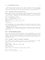
Let us now give some examples of numerical functions. We start by defining some very simple
functions on numbers:
#let square x = x *. x;;
square : float -> float = <fun>
#square 2.0;;
- : float = 4.0
#square (2.0 /. 3.0);;
- : float = 0.444444444444
#let sum_of_squares (x,y) = square(x) +. square(y);;
sum_of_squares : float * float -> float = <fun>
#let half_pi = 3.14159 /. 2.0
#in sum_of_squares(cos(half_pi), sin(half_pi));;
- : float = 1.0
4.1. NUMBERS
23
We now develop a classical example: the computation of the root of a function by Newton’s
method. Newton’s method can be stated as follows: if y is an approximation to a root of a function
f , then:
f (y)
y− 0
f (y)
is a better approximation, where f 0 (y) is the derivative of f evaluated at y. For example, with
f (x) = x2 − a, we have f 0 (x) = 2x, and therefore:
y−
y+
f (y)
y2 − a
=
y
−
=
0
f (y)
2y
2
a
y
We can define a function deriv for approximating the derivative of a function at a given point
by:
#let deriv f x dx = (f(x+.dx) -. f(x)) /. dx;;
deriv : (float -> float) -> float -> float -> float = <fun>
Provided dx is sufficiently small, this gives a reasonable estimate of the derivative of f at x.
The following function returns the absolute value of its floating point number argument. It uses
the “if . . . then . . . else” conditional construct.
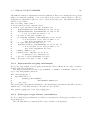
#let abs x = if x >. 0.0 then x else -. x;;
abs : float -> float = <fun>
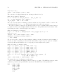
The main function, given below, uses three local functions. The first one, until, is an example
of a recursive function: it calls itself in its body, and is defined using a let rec construct (rec
shows that the definition is recursive). It takes three arguments: a predicate p on floats, a function
change from floats to floats, and a float x. If p(x) is false, then until is called with last argument
change(x), otherwise, x is the result of the whole call. We will study recursive functions more
closely later. The two other auxiliary functions, satisfied and improve, take a float as argument
and deliver respectively a boolean value and a float. The function satisfied asks wether the image
of its argument by f is smaller than epsilon or not, thus testing wether y is close enough to a root
of f. The function improve computes the next approximation using the formula given below. The
three local functions are defined using a cascade of let constructs. The whole function is:
#let newton f epsilon =
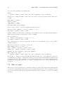
# let rec until p change x =
#
if p(x) then x
#
else until p change (change(x)) in
# let satisfied y = abs(f y) <. epsilon in
# let improve y = y -. (f(y) /. (deriv f y epsilon))
#in until satisfied improve;;
newton : (float -> float) -> float -> float -> float = <fun>
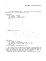
Some examples of equation solving:
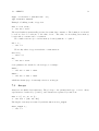
#let square_root x epsilon =
#
newton (function y -> y*.y -. x) epsilon x
24
CHAPTER 4. BASIC TYPES
#and cubic_root x epsilon =
#
newton (function y -> y*.y*.y -. x) epsilon x;;
square_root : float -> float -> float = <fun>
cubic_root : float -> float -> float = <fun>
#square_root 2.0 1e-5;;
- : float = 1.41421569553
#cubic_root 8.0 1e-5;;
- : float = 2.00000000131
#2.0 *. (newton cos 1e-5 1.5);;
- : float = 3.14159265359
4.2
Boolean values
The presence of the conditional construct implies the presence of boolean values. The type bool is
composed of two values true and false.
#true;;
- : bool = true
#false;;
- : bool = false
The functions with results of type bool are often called predicates. Many predicates are predefined
in Caml. Here are some of them:
#prefix <;;
- : ’a -> ’a -> bool = <fun>
#1 < 2;;
- : bool = true
#prefix <.;;
- : float -> float -> bool = <fun>
#3.14159 <. 2.718;;
- : bool = false
There exist also <=, >, >=, and similarly <=., >., >=..
4.2.1
Equality
Equality has a special status in functional languages because of functional values. It is easy to test
equality of values of base types (integers, floating-point numbers, booleans, . . . ):
#1 = 2;;
- : bool = false
#false = (1>2);;
- : bool = true
4.2. BOOLEAN VALUES
25
But it is impossible, in the general case, to decide the equality of functional values. Hence, equality
stops on a run-time error when it encounters functional values.
#(fun x -> x) = (fun x -> x);;
Uncaught exception: Invalid_argument "equal: functional value"
Since equality may be used on values of any type, what is its type? Equality takes two arguments
of the same type (whatever type it is) and returns a boolean value. The type of equality is a
polymorphic type, i.e. may take several possible forms. Indeed, when testing equality of two
numbers, then its type is int -> int -> bool, and when testing equality of strings, its type is
string -> string -> bool.
#prefix =;;
- : ’a -> ’a -> bool = <fun>
The type of equality uses type variables, written ’a, ‘b, etc. Any type can be substituted to type
variables in order to produces specific instances of types. For example, substituting int for ’a
above produces int -> int -> bool, which is the type of the equality function used on integer
values.
#1=2;;
- : bool = false
#(1,2) = (2,1);;
- : bool = false
#1 = (1,2);;
Toplevel input:
>1 = (1,2);;
>
^^^
This expression has type int * int,
but is used with type int.
4.2.2
Conditional
Conditional expressions are of the form “if etest then e1 else e2 ”, where etest is an expression of
type bool and e1 , e2 are expressions possessing the same type. As an example, the logical negation
could be written:
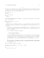
#let negate a = if a then false else true;;
negate : bool -> bool = <fun>
#negate (1=2);;
- : bool = true
26
4.2.3
CHAPTER 4. BASIC TYPES
Logical operators
The classical logical operators are available in Caml. Disjunction and conjunction are respectively
written or and &:
#true or false;;
- : bool = true
#(1<2) & (2>1);;
- : bool = true
The operators & and or are not functions. They should not be seen as regular functions, since they
evaluate their second argument only if it is needed. For example, the or operator evaluates its
second operand only if the first one evaluates to false. The behavior of these operators may be
described as follows:
e1 or e2
e1 & e2
is equivalent to
is equivalent to
if e1 then true else e2
if e1 then e2 else false
Negation is predefined:
#not true;;
- : bool = false
The not identifier receives a special treatment from the parser: the application “not f x” is
recognized as “not (f x)” while “f g x” is identical to “(f g) x”. This special treatment explains
why the functional value associated to not can be obtained only using the prefix keyword:
#prefix not;;
- : bool -> bool = <fun>
4.3
Strings and characters
String constants (type string) are written between " characters (double-quotes). Single-character
constants (type char) are written between ‘ characters (backquotes). The most used string operation is string concatenation, denoted by the ^ character.
#"Hello" ^ " World!";;
- : string = "Hello World!"
#prefix ^;;
- : string -> string -> string = <fun>
Characters are ASCII characters:
#‘a‘;;
- : char = ‘a‘
#‘\065‘;;
- : char = ‘A‘
4.4. TUPLES
27
and can be built from their ASCII code as in:
#char_of_int 65;;
- : char = ‘A‘
Other operations are available (sub_string, int_of_char, etc). See the Caml Light reference
manual [21] for complete information.
4.4
Tuples
4.4.1
Constructing tuples
It is possible to combine values into tuples (pairs, triples, . . . ). The value constructor for tuples is
the “,” character (the comma). We will often use parentheses around tuples in order to improve
readability, but they are not strictly necessary.
#1,2;;
- : int * int = 1, 2
#1,2,3,4;;
- : int * int * int * int = 1, 2, 3, 4
#let p = (1+2, 1<2);;
p : int * bool = 3, true
The infix “*” identifier is the type constructor for tuples. For instance, t1 ∗t2 corresponds to the
mathematical cartesian product of types t1 and t2 .
We can build tuples from any values: the tuple value constructor is generic.
4.4.2
Extracting pair components
Projection functions are used to extract components of tuples. For pairs, we have:
#fst;;
- : ’a * ’b -> ’a = <fun>
#snd;;
- : ’a * ’b -> ’b = <fun>
They have polymorphic types, of course, since they may be applied to any kind of pair. They are
predefined in the Caml system, but could be defined by the user (in fact, the cartesian product
itself could be defined — see section 6.1, dedicated to user-defined product types):
#let first (x,y) = x
#and second (x,y) = y;;
first : ’a * ’b -> ’a = <fun>
second : ’a * ’b -> ’b = <fun>
#first p;;
- : int = 3
#second p;;
- : bool = true
28
CHAPTER 4. BASIC TYPES
We say that first is a generic value because it works uniformly on several kinds of arguments
(provided they are pairs). We often confuse between “generic” and “polymorphic”, saying that
such value is polymorphic instead of generic.
4.5
Patterns and pattern-matching
Patterns and pattern-matching play an important role in ML languages. They appear in all real
programs and are strongly related to types (predefined or user-defined).
A pattern indicates the shape of a value. Patterns are “values with holes”. A single variable
(formal parameter) is a pattern (with no shape specified: it matches any value). When a value
is matched against a pattern (this is called pattern-matching), the pattern acts as a filter. We
already used patterns and pattern-matching in all the functions we wrote: the function body
(function x -> ...) does (trivial) pattern-matching. When applied to a value, the formal
parameter x gets bound to that value. The function body (function (x,y) -> x+y) does also
pattern-matching: when applied to a value (a pair, because of well-typing hypotheses), the x and
y get bound respectively to the first and the second component of that pair.
All these pattern-matching examples were trivial ones, they did not involve any test:
• formal parameters such as x do not impose any particular shape to the value they are supposed
to match;
• pair patterns such as (x,y) always match for typing reasons (cartesian product is a product
type).
However, some types do not guarantee such a uniform shape to their values. Consider the bool
type: an element of type bool is either true or false. If we impose to a value of type bool to
have the shape of true, then pattern-matching may fail. Consider the following function:
#let f =
Toplevel
>let f =
>
Warning:
f : bool
function true -> false;;
input:
function true -> false;;
^^^^^^^^^^^^^^^^^^^^^^
this matching is not exhaustive.
-> bool = <fun>
The compiler warns us that the pattern-matching may fail (we did not consider the false case).
Thus, if we apply f to a value that evaluates to true, pattern-matching will succeed (an equality
test is performed during execution).
#f (1<2);;
- : bool = false
But, if f’s argument evaluates to false, a run-time error is reported:
#f (1>2);;
Uncaught exception: Match_failure ("", 1346, 1368)
Here is a correct definition using pattern-matching:
4.5. PATTERNS AND PATTERN-MATCHING
29
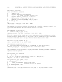
#let negate = function true -> false
#
| false -> true;;
negate : bool -> bool = <fun>
The pattern-matching has now two cases, separated by the “|” character. Cases are examined in
turn, from top to bottom. An equivalent definition of negate would be:
#let negate = function true -> false
#
| x -> true;;
negate : bool -> bool = <fun>
The second case now matches any boolean value (in fact, only false since true has been caught by
the first match case). When the second case is chosen, the identifier x gets bound to the argument
of negate, and could be used in the right-hand part of the match case. Since in our example we
do not use the value of the argument in the right-hand part of the second match case, another
equivalent definition of negate would be:
#let negate = function true -> false
#
| _ -> true;;
negate : bool -> bool = <fun>
Where “_” acts as a formal paramenter (matches any value), but does not introduce any binding:
it should be read as “anything else”.
As an example of pattern-matching, consider the following function definition (truth value table
of implication):
#let imply = function (true,true) -> true
#
| (true,false) -> false
#
| (false,true) -> true
#
| (false,false) -> true;;
imply : bool * bool -> bool = <fun>
Here is another way of defining imply, by using variables:
#let imply = function (true,x) -> x
#
| (false,x) -> true;;
imply : bool * bool -> bool = <fun>
Simpler, and simpler again:
#let imply = function (true,x) -> x
#
| (false,_) -> true;;
imply : bool * bool -> bool = <fun>
#let imply = function (true,false) -> false
#
| _ -> true;;
imply : bool * bool -> bool = <fun>
Pattern-matching is allowed on any type of value (non-trivial pattern-matching is only possible on
types with data constructors).
For example:
30
CHAPTER 4. BASIC TYPES
#let is_zero = function 0 -> true | _ -> false;;
is_zero : int -> bool = <fun>
#let is_yes = function "oui" -> true
#
| "si" -> true
#
| "ya" -> true
#
| "yes" -> true
#
| _ -> false;;
is_yes : string -> bool = <fun>
4.6
Functions
The type constructor “->” is predefined and cannot be defined in ML’s type system. We shall
explore in this section some further aspects of functions and functional types.
4.6.1
Functional composition
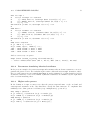
Functional composition is easily definable in Caml. It is of course a polymorphic function:
#let compose f g = function x -> f (g (x));;
compose : (’a -> ’b) -> (’c -> ’a) -> ’c -> ’b = <fun>
The type of compose contains no more constraints than the ones appearing in the definition: in a
sense, it is the most general type compatible with these constraints.
These constraints are:
• the codomain of g and the domain of f must be the same;
• x must belong to the domain of g;
• compose f g x will belong to the codomain of f.
Let’s see compose at work:
#let succ x = x+1;;
succ : int -> int = <fun>
#compose succ list_length;;
- : ’_a list -> int = <fun>
#(compose succ list_length) [1;2;3];;
- : int = 4
4.6.2
Currying
We can define two versions of the addition function:
4.6. FUNCTIONS
31
#let plus = function (x,y) -> x+y;;
plus : int * int -> int = <fun>
#let add = function x -> (function y -> x+y);;
add : int -> int -> int = <fun>
These two functions differ only in their way of taking their arguments. The first one will take an
argument belonging to a cartesian product, the second one will take a number and return a function.
The add function is said to be the curried version of plus (in honor of the logician Haskell Curry).
The currying transformation may be written in Caml under the form of a higher-order function:
#let curry f = function x -> (function y -> f(x,y));;
curry : (’a * ’b -> ’c) -> ’a -> ’b -> ’c = <fun>
Its inverse function may be defined by:
#let uncurry f = function (x,y) -> f x y;;
uncurry : (’a -> ’b -> ’c) -> ’a * ’b -> ’c = <fun>
We may check the types of curry and uncurry on particular examples:
#uncurry (prefix +);;
- : int * int -> int = <fun>
#uncurry (prefix ^);;
- : string * string -> string = <fun>
#curry plus;;
- : int -> int -> int = <fun>
Exercises
Exercise 4.1 Define functions that compute the surface area and the volume of well-known geometric objects (rectangles, circles, spheres, . . . ).
Exercise 4.2 What would happen in a language submitted to call-by-value with recursion if there
was no conditional construct (if ... then ... else ...)?
Exercise 4.3 Define the factorial function such that:
factorial n = n ∗ (n − 1) ∗ . . . ∗ 2 ∗ 1
Give two versions of factorial: recursive and tail recursive.
Exercise 4.4 Define the fibonacci function that, when given a number n, returns the nth Fibonacci number, i.e. the nth term un of the sequence defined by:
u1 = 1
u2 = 1
un+2 = un+1 + un
32
CHAPTER 4. BASIC TYPES
Exercise 4.5 What are the types of the following expressions?
• uncurry compose
• compose curry uncurry
• compose uncurry curry
Chapter 5
Lists
Lists represent an important data structure, mainly because of their success in the Lisp language.
Lists in ML are homogeneous: a list cannot contain elements of different types. This may be
annoying to new ML users, yet lists are not as fundamental as in Lisp, since ML provides a facility
for introducing new types allowing the user to define more precisely the data structures needed by
the program (cf. chapter 6).
5.1
Building lists
Lists are empty or non empty sequences of elements. They are built with two value constructors:
• [], the empty list (read: nil );
• ::, the non-empty list constructor (read: cons). It takes an element e and a list l, and builds
a new list whose first element (head ) is e and rest (tail ) is l.
The special syntax [e1 ; . . . ; en ] builds the list whose elements are e1 , . . . , en . It is equivalent to
e1 :: (e2 :: . . . (en :: []) . . .).
We may build lists of numbers:
#1::2::[];;
- : int list = [1; 2]
#[3;4;5];;
- : int list = [3; 4; 5]
#let x=2 in [1; 2; x+1; x+2];;
- : int list = [1; 2; 3; 4]
Lists of functions:
#let adds =
# let add x y = x+y
# in [add 1; add 2; add 3];;
adds : (int -> int) list = [<fun>; <fun>; <fun>]
33
34
CHAPTER 5. LISTS
and indeed, lists of anything desired.
We may wonder what are the types of the list (data) constructors. The empty list is a list of
anything (since it has no element), it has thus the type “list of anything”. The list constructor ::
takes an element and a list (containing elements with the same type) and returns a new list. Here
again, there is no type constraint on the elements considered.
#[];;
- : ’a list = []
#function head -> function tail -> head::tail;;
- : ’a -> ’a list -> ’a list = <fun>
We see here that the list type is a recursive type. The :: constructor receives two arguments;
the second argument is itself a list.
5.2
Extracting elements from lists: pattern-matching
We know how to build lists; we now show how to test emptiness of lists (although the equality
predicate could be used for that) and extract elements from lists (e.g. the first one). We have used
pattern-matching on pairs, numbers or boolean values. The syntax of patterns also includes list
patterns. (We will see that any data constructor can actually be used in a pattern.) For lists, at
least two cases have to be considered (empty, non empty):
#let is_null = function [] -> true | _ -> false;;
is_null : ’a list -> bool = <fun>
#let head = function x::_ -> x
#
| _ -> raise (Failure "head");;
head : ’a list -> ’a = <fun>
#let tail = function _::l -> l
#
| _ -> raise (Failure "tail");;
tail : ’a list -> ’a list = <fun>
The expression raise (Failure "head") will produce a run-time error when evaluated. In the
definition of head above, we have chosen to forbid taking the head of an empty list. We could have
chosen tail [] to evaluate to [], but we cannot return a value for head [] without changing the
type of the head function.
We say that the types list and bool are sum types, because they are defined with several
alternatives:
• a list is either [] or :: of . . .
• a boolean value is either true or false
Lists and booleans are typical examples of sum types. Sum types are the only types whose
values need run-time tests in order to be matched by a non-variable pattern (i.e. a pattern that is
not a single variable).
The cartesian product is a product type (only one alternative). Product types do not involve runtime tests during pattern-matching, because the type of their values suffices to indicate statically
what their structure is.
5.3. FUNCTIONS OVER LISTS
5.3
35
Functions over lists
We will see in this section the definition of some useful functions over lists. These functions are of
general interest, but are not exhaustive. Some of them are predefined in the Caml Light system.
See also [9] or [37] for other examples of functions over lists.
Computation of the length of a list:
#let rec length = function [] -> 0
#
| _::l -> 1 + length(l);;
length : ’a list -> int = <fun>
#length [true; false];;
- : int = 2
Concatenating two lists:
#let rec append =
#
function [], l2 -> l2
#
| (x::l1), l2 -> x::(append (l1,l2));;
append : ’a list * ’a list -> ’a list = <fun>
The append function is already defined in Caml, and bound to the infix identifier @.
#[1;2] @ [3;4];;
- : int list = [1; 2; 3; 4]
Reversing a list:
#let rec rev = function [] -> []
#
| x::l -> (rev l) @ [x];;
rev : ’a list -> ’a list = <fun>
#rev [1;2;3];;
- : int list = [3; 2; 1]
The map function applies a function on all the elements of a list, and return the list of the function
results. It demonstrates full functionality (it takes a function as argument), list processing, and
polymorphism (note the sharing of type variables between the arguments of map in its type).
#let rec map f =
#
function [] -> []
#
| x::l -> (f x)::(map f l);;
map : (’a -> ’b) -> ’a list -> ’b list = <fun>
#map (function x -> x+1) [1;2;3;4;5];;
- : int list = [2; 3; 4; 5; 6]
#map length [ [1;2;3]; [4;5]; [6]; [] ];;
- : int list = [3; 2; 1; 0]
36
CHAPTER 5. LISTS
The following function is a list iterator. It takes a function f , a base element a and a list
[x1 ;. . . ;xn ]. It computes:
it list f a [x1 ; . . . ; xn ] = f (. . . (f (f a x1 ) x2 ) . . .)xn
For instance, when applied to the curried addition function, to the base element 0, and to a list of
numbers, it computes the sum of all elements in the list. The expression:
it_list (prefix +) 0 [1;2;3;4;5]
evaluates to ((((0+1)+2)+3)+4)+5
i.e. to 15.
#let rec it_list f a =
#
function [] -> a
#
| x::l -> it_list f (f a x) l;;
it_list : (’a -> ’b -> ’a) -> ’a -> ’b list -> ’a = <fun>
#let sigma = it_list prefix + 0;;
sigma : int list -> int = <fun>
#sigma [1;2;3;4;5];;
- : int = 15
#it_list (prefix *) 1 [1;2;3;4;5];;
- : int = 120
The it_list function is one of the many ways to iterate over a list. For other list iteration
functions, see [9].
Exercises
Exercise 5.1 Define the combine function which, when given a pair of lists, returns a list of pairs
such that:
combine ([x1;...;xn],[y1;...;yn]) = [(x1,y1);...;(xn,yn)]
The function generates a run-time error if the argument lists do not have the same length.
Exercise 5.2 Define a function which, when given a list, returns the list of all its sublists.
Chapter 6
User-defined types
The user is allowed to define his/her own data types. With this facility, there is no need to encode
the data structures that must be manipulated by a program into lists (as in Lisp) or into arrays (as
in Fortran). Furthermore, early detection of type errors is enforced, since user-defined data types
reflect precisely the needs of the algorithms.
Types are either:
• product types,
• or sum types.
We have already seen examples of both kinds of types: the bool and list types are sum types
(they contain values with different shapes and are defined and matched using several alternatives).
The cartesian product is an example of a product type: we know statically the shape of values
belonging to cartesian products.
In this chapter, we will see how to define and use new types in Caml.
6.1
Product types
Product types are finite labeled products of types. They are a generalization of cartesian product.
Elements of product types are called records.
6.1.1
Defining product types
An example: suppose we want to define a data structure containing information about individuals.
We could define:
#let jean=("Jean",23,"Student","Paris");;
jean : string * int * string * string = "Jean", 23, "Student", "Paris"
and use pattern-matching to extract any particular information about the person jean. The problem with such usage of cartesian product is that a function name_of returning the name field of
a value representing an individual would have the same type as the general first projection for
4-tuples (and indeed would be the same function). This type is not precise enough since it allows
for the application of the function to any 4-uple, and not only to values such as jean.
Instead of using cartesian product, we define a person data type:
37
38
CHAPTER 6. USER-DEFINED TYPES
#type person =
# {Name:string; Age:int; Job:string; City:string};;
Type person defined.
The type person is the product of string, int, string and string. The field names provide type
information and also documentation: it is much easier to understand data structures such as jean
above than arbitrary tuples.
We have labels (i.e. Name, . . . ) to refer to components of the products. The order of appearance
of the products components is not relevant: labels are sufficient to uniquely identify the components.
The Caml system finds a canonical order on labels to represent and print record values. The order
is always the order which appeared in the definition of the type.
We may now define the individual jean as:
#let jean = {Job="Student"; City="Paris";
#
Name="Jean"; Age=23};;
jean : person = {Name = "Jean"; Age = 23; Job = "Student"; City = "Paris"}
This example illustrates the fact that order of labels is not relevant.
6.1.2
Extracting products components
The canonical way of extracting product components is pattern-matching. Pattern-matching provides a way to mention the shape of values and to give (local) names to components of values. In
the following example, we name n the numerical value contained in the field Age of the argument,
and we choose to forget values contained in other fields (using the _ character).
#let age_of = function
#
{Age=n; Name=_; Job=_; City=_} -> n;;
age_of : person -> int = <fun>
#age_of jean;;
- : int = 23
It is also possible to access the value of a single field, with the . (dot) operator:
#jean.Age;;
- : int = 23
#jean.Job;;
- : string = "Student"
Labels always refer to the most recent type definition: when two record types possess some common
labels, then these labels always refer to the most recently defined type. When using modules (see
section 11.2) this problem arises for types defined in the same module. For types defined in different
modules, the full name of labels (i.e. with the name of the modules prepended) disambiguates such
situations.
6.2. SUM TYPES
6.1.3
39
Parameterized product types
It is important to be able to define parameterized types in order to define generic data structures.
The list type is parameterized, and this is the reason why we may build lists of any kind of values.
If we want to define the cartesian product as a Caml type, we need type parameters because we
want to be able to build cartesian product of any pair of types.
#type (’a,’b) pair = {Fst:’a; Snd:’b};;
Type pair defined.
#let first x = x.Fst and second x = x.Snd;;
first : (’a, ’b) pair -> ’a = <fun>
second : (’a, ’b) pair -> ’b = <fun>
#let p={Snd=true; Fst=1+2};;
p : (int, bool) pair = {Fst = 3; Snd = true}
#first(p);;
- : int = 3
Warning: the pair type is similar to the Caml cartesian product *, but it is a different type.
#fst p;;
Toplevel input:
>fst p;;
>
^
This expression has type (int, bool) pair,
but is used with type ’a * ’b.
Actually, any two type definitions produce different types. If we enter again the previous definition:
#type (’a,’b) pair = {Fst:’a; Snd:’b};;
Type pair defined.
we cannot any longer extract the Fst component of x:
#p.Fst;;
Toplevel input:
>p.Fst;;
>^
This expression has type (int, bool) pair,
but is used with type (’a, ’b) pair.
since the label Fst refers to the latter type pair that we defined, while p’s type is the former pair.
6.2
Sum types
A sum type is the finite labeled disjoint union of several types. A sum type definition defines a type
as being the union of some other types.
40
CHAPTER 6. USER-DEFINED TYPES
6.2.1
Defining sum types
Example: we want to have a type called identification whose values can be:
• either strings (name of an individual),
• or integers (encoding of social security number as a pair of integers).
We then need a type containing both int * int and character strings. We also want to preserve
static type-checking, we thus want to be able to distinguish pairs from character strings even if
they are injected in order to form a single type.
Here is what we would do:
#type identification = Name of string
#
| SS of int * int;;
Type identification defined.
The type identification is the labeled disjoint union of string and int * int. The labels
Name and SS are injections. They respectively inject int * int and string into a single type
identification.
Let us use these injections in order to build new values:
#let id1 = Name "Jean";;
id1 : identification = Name "Jean"
#let id2 = SS (1670728,280305);;
id2 : identification = SS (1670728, 280305)
Values id1 and id2 belong to the same type. They may for example be put into lists as in:
#[id1;id2];;
- : identification list = [Name "Jean"; SS (1670728, 280305)]
Injections may possess one argument (as in the example above), or none. The latter case
corresponds1 to enumerated types, as in Pascal. An example of enumerated type is:
#type suit = Heart
#
| Diamond
#
| Club
#
| Spade;;
Type suit defined.
#Club;;
- : suit = Club
The type suit contains only 4 distinct elements. Let us continue this example by defining a type
for cards.
1
In Caml Light, there is no implicit order on values of sum types.
6.2. SUM TYPES
41
#type card = Ace of suit
#
| King of suit
#
| Queen of suit
#
| Jack of suit
#
| Plain of suit * int;;
Type card defined.
The type card is the disjoint union of:
• suit under the injection Ace,
• suit under the injection King,
• suit under the injection Queen,
• suit under the injection Jack,
• the product of int and suit under the injection Plain.
Let us build a list of cards:
#let figures_of c = [Ace c; King c; Queen c; Jack c]
#and small_cards_of c =
#
map (function n -> Plain(c,n)) [7;8;9;10];;
figures_of : suit -> card list = <fun>
small_cards_of : suit -> card list = <fun>
#figures_of Heart;;
- : card list = [Ace Heart; King Heart; Queen Heart; Jack Heart]
#small_cards_of Spade;;
- : card list =
[Plain (Spade, 7); Plain (Spade, 8); Plain (Spade, 9); Plain (Spade, 10)]
6.2.2
Extracting sum components
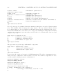
Of course, pattern-matching is used to extract sum components. In case of sum types, patternmatching uses dynamic tests for this extraction. The next example defines a function color returning the name of the color of the suit argument:
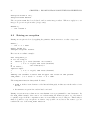
#let color = function Diamond -> "red"
#
| Heart -> "red"
#
| _ -> "black";;
color : suit -> string = <fun>
Let us count the values of cards (assume we are playing “belote”):
#let count trump = function
#
Ace _
-> 11
# | King _
-> 4
42
CHAPTER 6. USER-DEFINED TYPES
# | Queen _
-> 3
# | Jack c
-> if c = trump then 20 else 2
# | Plain (c,10) -> 10
# | Plain (c,9) -> if c = trump then 14 else 0
# | _
-> 0;;
count : suit -> card -> int = <fun>
6.2.3
Recursive types
Some types possess a naturally recursive structure, lists, for example. It is also the case for tree-like
structures, since trees have subtrees that are trees themselves.
Let us define a type for abstract syntax trees of a simple arithmetic language2 . An arithmetic
expression will be either a numeric constant, or a variable, or the addition, multiplication, difference,
or division of two expressions.
#type arith_expr = Const of int
#
| Var of string
#
| Plus of args
#
| Mult of args
#
| Minus of args
#
| Div of args
#and args = {Arg1:arith_expr; Arg2:arith_expr};;
Type arith_expr defined.
Type args defined.
The two types arith_expr and args are simultaneously defined, and arith_expr is recursive since
its definition refers to args which itself refers to arith_expr. As an example, one could represent
the abstract syntax tree of the arithmetic expression “x+(3*y)” as the Caml value:
#Plus {Arg1=Var "x";
#
Arg2=Mult{Arg1=Const 3; Arg2=Var "y"}};;
- : arith_expr =
Plus {Arg1 = Var "x"; Arg2 = Mult {Arg1 = Const 3; Arg2 = Var "y"}}
The recursive definition of types may lead to types such that it is hard or impossible to build
values of these types. For example:
#type stupid = {Next:stupid};;
Type stupid defined.
Elements of this type are infinite data structures. Essentially, the only way to construct one is:
#let rec stupid_value = {Next=stupid_value};;
stupid_value : stupid =
{Next =
2
Syntax trees are said to be abstract because they are pieces of abstract syntax contrasting with concrete syntax
which is the “string” form of programs: analyzing (parsing) concrete syntax usually produces abstract syntax.
6.2. SUM TYPES
43
{Next =
{Next =
{Next =
{Next =
{Next =
{Next =
{Next =
{Next =
{Next =
{Next = {Next = {Next = {Next = {Next = {Next = .}}}}}}}}}}
}}}}}}
Recursive type definitions should be well-founded (i.e. possess a non-recursive case, or base
case) in order to work well with call-by-value.
6.2.4
Parameterized sum types
Sum types may also be parameterized. Here is the definition of a type isomorphic to the list type:
#type ’a sequence = Empty
#
| Sequence of ’a * ’a sequence;;
Type sequence defined.
A more sophisticated example is the type of generic binary trees:
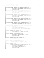
#type (’a,’b) btree = Leaf of ’b
#
| Btree of (’a,’b) node
#and (’a,’b) node = {Op:’a;
#
Son1: (’a,’b) btree;
#
Son2: (’a,’b) btree};;
Type btree defined.
Type node defined.
A binary tree is either a leaf (holding values of type ’b) or a node composed of an operator (of
type ’a) and two sons, both of them being binary trees.
Binary trees can also be used to represent abstract trees for arithmetic expressions (with only
binary operators and only one kind of leaves). The abstract syntax tree t of “1+2” could be defined
as:
#let t = Btree {Op="+"; Son1=Leaf 1; Son2=Leaf 2};;
t : (string, int) btree = Btree {Op = "+"; Son1 = Leaf 1; Son2 = Leaf 2}
Finally, it is time to notice that pattern-matching is not restricted to function bodies, i.e.
constructs such as:
function
|
|
P1
...
Pn
-> E1
-> En
44
CHAPTER 6. USER-DEFINED TYPES
but there is also a construct dedicated to pattern-matching of actual values:
match E with
|
|
P1
...
Pn
-> E1
-> En
which matches the value of the expression E against each of the patterns Pi , selecting the first one
that matches, and giving control to the corresponding expression. For example, we can match the
tree t previously defined by:
#match t with Btree{Op=x; Son1=_; Son2=_} -> x
#
| Leaf l -> "No operator";;
- : string = "+"
6.2.5
Data constructors and functions
One may ask: “What is the difference between a sum data constructor and a function?”. At first
sight, they look very similar. We assimilate constant data constructors (such as Heart) to constants.
Similarly, in Caml Light, sum data constructors with arguments also possess a functional type:
#Ace;;
- : suit -> card = <fun>
However, a data constructor possesses particular properties that a general function does not possess,
and it is interesting to understand these differences. From the mathematical point of view, a sum
data constructor is known to be an injection while a Caml function is a general function without
further information. A mathematical injection f : A → B admits an inverse function f −1 from its
image f (A) ⊂ B to A.
From the examples above, if we consider the King constructor, then:
#let king c = King c;;
king : suit -> card = <fun>
king is the general function associated to the King constructor, and:
#function King c -> c;;
Toplevel input:
>function King c -> c;;
>^^^^^^^^^^^^^^^^^^^^
Warning: this matching is not exhaustive.
- : card -> suit = <fun>
is the inverse function for king. It is a partial function, since pattern-matching may fail.
6.2.6
Degenerate cases: when sums meet products
What is the status of a sum type with a single case such as:
#type counter1 = Counter of int;;
Type counter1 defined.
6.3. SUMMARY
45
Of course, the type counter1 is isomorphic to int. The injection function x -> Counter x is a
total function from int to counter1. It is thus a bijection.
Another way to define a type isomorphic to int would be:
#type counter2 = {Counter: int};;
Type counter2 defined.
The types counter1 and counter2 are isomorphic to int. They are at the same time sum and
product types. Their pattern-matching does not perform any run-time test.
The possibility of defining arbitrary complex data types permits the easy manipulation of abstract syntax trees in Caml (such as the arith_expr type above). These abstract syntax trees are
supposed to represent programs of a language (e.g. a language of arithmetic expressions). These
kind of languages which are defined in Caml are called object-languages and Caml is said to be
their metalanguage.
6.3
Summary
• New types can be introduced in Caml.
• Types may be parameterized by type variables. The syntax of type parameters is:
<params> ::
| <tvar>
| ( <tvar> [, <tvar>]* )
• Types can be recursive.
• Product types:
– Mathematical product of several types.
– The construct is:
type <params> <tname> =
{<Field>: <type>; ...}
where the <type>s may contain type variables appearing in <params>.
• Sum types:
– Mathematical disjoint union of several types.
– The construct is:
type <params> <tname> =
<Injection> [of <type>] | ...
where the <type>s may contain type variables appearing in <params>.
46
CHAPTER 6. USER-DEFINED TYPES
Exercises
Exercise 6.1 Define a function taking as argument a binary tree and returning a pair of lists: the
first one contains all operators of the tree, the second one contains all its leaves.
Exercise 6.2 Define a function map_btree analogous to the map function on lists. The function
map_btree should take as arguments two functions f and g, and a binary tree. It should return a
new binary tree whose leaves are the result of applying f to the leaves of the tree argument, and
whose operators are the results of applying the g function to the operators of the argument.
Exercise 6.3 We can associate to the list type definition an canonical iterator in the following
way. We give a functional interpretation to the data constructors of the list type.
We change the list constructors [] and :: respectively into a constant a and an operator ⊕
(used as a prefix identifier), and abstract with respect to these two operators, obtaining the list
iterator satisfying:
list it ⊕ a [] = a
list it ⊕ a (x1 ::. . . ::xn ::[]) = x1 ⊕ (. . . ⊕ (xn ⊕ a). . . )
Its Caml definition would be:
#let rec list_it f a =
#
function [] -> a
#
| x::l -> f x (list_it f a l);;
list_it : (’a -> ’b -> ’b) -> ’b -> ’a list -> ’b = <fun>
As an example, the application of it_list to the functional composition and to its neutral element
(the identity function), computes the composition of lists of functions (try it!).
Define, using the same method, a canonical iterator over binary trees.
Part II
Caml Light specifics
47
Chapter 7
Mutable data structures
The definition of a sum or product type may be annotated to allow physical (destructive) update
on data structures of that type. This is the main feature of the imperative programming style.
Writing values into memory locations is the fundamental mechanism of imperative languages such
as Pascal. The Lisp language, while mostly functional, also provides the dangerous functions rplaca
and rplacd to physically modify lists. Mutable structures are required to implement many efficient
algorithms. They are also very convenient to represent the current state of a state machine.
7.1
User-defined mutable data structures
Assume we want to define a type person as in the previous chapter. Then, it seems natural to
allow a person to change his/her age, job and the city that person lives in, but not his/her name.
We can do this by annotating some labels in the type definition of person by the mutable keyword:
#type person =
#
{Name: string; mutable Age: int;
#
mutable Job: string; mutable City: string};;
Type person defined.
We can build values of type person in the very same way as before:
#let jean =
#
{Name="Jean"; Age=23; Job="Student"; City="Paris"};;
jean : person = {Name = "Jean"; Age = 23; Job = "Student"; City = "Paris"}
But now, the value jean may be physically modified in the fields specified to be mutable in the
definition (and only in these fields).
We can modify the field Field of an expression <expr1> in order to assign it the value of
<expr2> by using the following construct:
<expr1>.Field <- <expr2>
For example; if we want jean to become one year older, we would write:
#jean.Age <- jean.Age + 1;;
- : unit = ()
49
50
CHAPTER 7. MUTABLE DATA STRUCTURES
Now, the value jean has been modified into:
#jean;;
- : person = {Name = "Jean"; Age = 24; Job = "Student"; City = "Paris"}
We may try to change the Name of jean, but we won’t succeed: the typecheker will not allow us to
do that.
#jean.Name <- "Paul";;
Toplevel input:
>jean.Name <- "Paul";;
>^^^^^^^^^^^^^^^^^^^
The label Name is not mutable.
It is of course possible to use such constructs in functions as in:
#let get_older ({Age=n; _} as p) = p.Age <- n + 1;;
get_older : person -> unit = <fun>
In that example, we named n the current Age of the argument, but we also named p the argument.
This is an alias pattern: it saves us the bother of writing:
#let get_older p =
#
match p with {Age=n} -> p.Age <- n + 1;;
get_older : person -> unit = <fun>
Notice that in the two previous expressions, we did not specify all fields of the record p. Other
examples would be:
#let move p new_city = p.City <- new_city
#and change_job p j = p.Job <- j;;
move : person -> string -> unit = <fun>
change_job : person -> string -> unit = <fun>
#change_job jean "Teacher"; move jean "Cannes";
#get_older jean; jean;;
- : person = {Name = "Jean"; Age = 25; Job = "Teacher"; City = "Cannes"}
We used the “;” character between the different changes we imposed to jean. This is the sequencing
of evaluations: it permits to evaluate successively several expressions, discarding the result of each
(except the last one). This construct becomes useful in the presence of side-effects such as physical
modifications and input/output, since we want to explicitly specify the order in which they are
performed.
7.2
The ref type
The ref type is the predefined type of mutable indirection cells. It is present in the Caml system
for reasons of compatibility with earlier versions of Caml. The ref type could be defined as follows
(we don’t use the ref name in the following definition because we want to preserve the original
ref type):
7.3. ARRAYS
51
#type ’a reference = {mutable Ref: ’a};;
Type reference defined.
Example of building a value of type ref:
#let r = ref (1+2);;
r : int ref = ref 3
The ref identifier is syntactically presented as a sum data constructor. The definition of r should
be read as “let r be a reference to the value of 1+2”. The value of r is nothing but a memory
location whose contents can be overwritten.
We consult a reference (i.e. read its memory location) with the “!” symbol:
#!r + 1;;
- : int = 4
We modify values of type ref with the := infix function:
#r:=!r+1;;
- : unit = ()
#r;;
- : int ref = ref 4
Some primitives are attached to the ref type, for example:
#incr;;
- : int ref -> unit = <fun>
#decr;;
- : int ref -> unit = <fun>
which increments (resp. decrements) references on integers.
7.3
Arrays
Arrays are modifiable data structures. They belong to the parameterized type ’a vect. Array
expressions are bracketed by [| and |], and elements are separated by semicolons:
#let a = [| 10; 20; 30 |];;
a : int vect = [|10; 20; 30|]
The length of an array is returned by with the function vect_length:
#vect_length a;;
- : int = 3
52
7.3.1
CHAPTER 7. MUTABLE DATA STRUCTURES
Accessing array elements
Accesses to array elements can be done using the following syntax:
#a.(0);;
- : int = 10
or, more generally: e1 .(e2 ), where e1 evaluates to an array and e2 to an integer. Alternatively, the
function vect_item is provided:
#vect_item;;
- : ’a vect -> int -> ’a = <fun>
The first element of an array is at index 0. Arrays are useful because accessing an element is done
in constant time: an array is a contiguous fragment of memory, while accessing list elements takes
linear time.
7.3.2
Modifying array elements
Modification of an array element is done with the construct:
e1 .(e2 ) <- e3
where e3 has the same type as the elements of the array e1 . The expression e2 computes the index
at which the modification will occur.
As for accessing, a function for modifying array elements is also provided:
#vect_assign;;
- : ’a vect -> int -> ’a -> unit = <fun>
For example:
#a.(0) <- (a.(0)-1);;
- : unit = ()
#a;;
- : int vect = [|9; 20; 30|]
#vect_assign a 0 ((vect_item a 0) - 1);;
- : unit = ()
#a;;
- : int vect = [|8; 20; 30|]
7.4
Loops: while and for
Imperative programming (i.e. using side-effects such as physical modification of data structures)
traditionally makes use of sequences and explicit loops. Sequencing evaluation in Caml Light is
done by using the semicolon “;”. Evaluating expression e1 , discarding the value returned, and then
evaluating e2 is written:
7.4. LOOPS: WHILE AND FOR
53
e1 ; e2
If e1 and e2 perform side-effects, this construct ensures that they will be performed in the specified
order (from left to right). In order to emphasize sequential side-effects, instead of using parentheses
around sequences, one can use begin and end, as in:
#let x = ref 1 in
# begin
#
x := !x + 1;
#
x := !x * !x
# end;;
- : unit = ()
The keywords begin and end are equivalent to opening and closing parentheses. The program
above could be written as:
#let x = ref 1 in
# (x := !x + 1; x := !x * !x);;
- : unit = ()
Explicit loops are not strictly necessary per se: a recursive function could perform the same
work. However, the usage of an explicit loop locally emphasizes a more imperative style. Two loops
are provided:
• while: while e1 do e2 done evaluates e1 which must return a boolean expression, if e1 return
true, then e2 (which is usually a sequence) is evaluated, then e1 is evaluated again and so on
until e1 returns false.
• for: two variants, increasing and decreasing
– for v=e1 to e2 do e3 done
– for v=e1 downto e2 do e3 done
where v is an identifier. Expressions e1 and e2 are the bounds of the loop: they must evaluate
to integers. In the case of the increasing loop, the expressions e1 and e2 are evaluated
producing values n1 and n2 : if n1 is strictly greater than n2 , then nothing is done. Otherwise,
e3 is evaluated (n2 − n1 ) + 1 times, with the variable v bound successively to n1 , n1 + 1, . . . ,
n2 .
The behavior of the decreasing loop is similar: if n1 is strictly smaller than n2 , then nothing
is done. Otherwise, e3 is evaluated (n1 − n2 ) + 1 times with v bound to successive values
decreasing from n1 to n2 .
Both loops return the value () of type unit.
#for i=0 to (vect_length a) - 1 do a.(i) <- i done;;
- : unit = ()
#a;;
- : int vect = [|0; 1; 2|]
54
7.5
CHAPTER 7. MUTABLE DATA STRUCTURES
Polymorphism and mutable data structures
There are some restrictions concerning polymorphism and mutable data structures. One cannot
enclose polymorphic objects inside mutable data structures.
#let r = ref [];;
r : ’_a list ref = ref []
The reason is that once the type of r, (’a list) ref, has been computed, it cannot be changed.
But the value of r can be changed: we could write:
r:=[1;2];;
and now, r would be a reference on a list of numbers while its type would still be (’a list) ref,
allowing us to write:
r:= true::!r;;
making r a reference on [true; 1; 2], which is an illegal Caml object.
Thus the Caml typechecker imposes that modifiable data structures appearing at toplevel must
possess monomorphic types (i.e. not polymorphic).
Exercises
Exercise 7.1 Give a mutable data type defining the Lisp type of lists and define the four functions
car, cdr, rplaca and rplacd.
Exercise 7.2 Define a stamp function, of type unit -> int, that returns a fresh integer each time
it is called. That is, the first call returns 1; the second call returns 2; and so on.
Exercise 7.3 Define a quick_sort function on arrays of floating point numbers following the
quicksort algorithm [13]. Information about the quicksort algorithm can be found in [33], for
example.
Chapter 8
Escaping from computations:
exceptions
In some situations, it is necessary to abort computations. If we are trying to compute the integer
division of an integer n by 0, then we must escape from that embarrassing situation without
returning any result.
Another example of the usage of such an escape mechanism appears when we want to define
the head function on lists:
#let head = function
#
x::L -> x
#
| [] -> raise (Failure "head: empty list");;
Toplevel input:
>
x::L -> x
>
^
Warning: the variable L starts with an upper case letter in this pattern.
head : ’a list -> ’a = <fun>
We cannot give a regular value to the expression head [] without losing the polymorphism of head.
We thus choose to escape: we raise an exception.
8.1
Exceptions
An exception is a Caml value of the built-in type exn, very similar to a sum type. An exception:
• has a name (Failure in our example),
• and holds zero or one value ("head:
empty list" of type string in the example).
Some exceptions are predefined, like Failure. New exceptions can be defined with the following
construct:
exception <exception name> [of <type>]
Example:
55
56
CHAPTER 8. ESCAPING FROM COMPUTATIONS: EXCEPTIONS
#exception Found of int;;
Exception Found defined.
The exception Found has been declared, and it carries integer values. When we apply it to an
integer, we get an exception value (of type exn):
#Found 5;;
- : exn = Found 5
8.2
Raising an exception
Raising an exception is done by applying the primitive function raise to a value of type exn:
#raise;;
- : exn -> ’a = <fun>
#raise (Found 5);;
Uncaught exception: Found 5
Here is a more realistic example:
#let find_index p =
# let rec find n =
#
function [] -> raise (Failure "not found")
#
| x::L -> if p(x) then raise (Found n)
#
else find (n+1) L
# in find 1;;
Toplevel input:
>
| x::L -> if p(x) then raise (Found n)
>
^
Warning: the variable L starts with an upper case letter in this pattern.
find_index : (’a -> bool) -> ’a list -> ’b = <fun>
The find_index function always fails. It raises:
• Found n, if there is an element x of the list such that p(x), in this case n is the index of x in
the list,
• the Failure exception if no such x has been found.
Raising exceptions is more than an error mechanism: it is a programmable control structure. In
the find_index example, there was no error when raising the Found exception: we only wanted
to quickly escape from the computation, since we found what we were looking for. This is why it
must be possible to trap exceptions: we want to trap possible errors, but we also want to get our
result in the case of the find_index function.
8.3. TRAPPING EXCEPTIONS
8.3
57
Trapping exceptions
Trapping exceptions is achieved by the following construct:
try <expression> with <match cases>
This construct evaluates <expression>. If no exception is raised during the evaluation, then
the result of the try construct is the result of <expression>. If an exception is raised during this
evaluation, then the raised exception is matched against the <match cases>. If a case matches,
then control is passed to it. If no case matches, then the exception is propagated outside of the
try construct, looking for the enclosing try.
Example:
#let find_index p L =
# let rec find n =
#
function [] -> raise (Failure "not found")
#
| x::L -> if p(x) then raise (Found n)
#
else find (n+1) L
# in
#
try find 1 L with Found n -> n;;
Toplevel input:
>let find_index p L =
>
^
Warning: the variable L starts with an upper case letter in this pattern.
Toplevel input:
>
| x::L -> if p(x) then raise (Found n)
>
^
Warning: the variable L starts with an upper case letter in this pattern.
find_index : (’a -> bool) -> ’a list -> int = <fun>
#find_index (function n -> (n mod 2) = 0) [1;3;5;7;9;10];;
- : int = 6
#find_index (function n -> (n mod 2) = 0) [1;3;5;7;9];;
Uncaught exception: Failure "not found"
The <match cases> part of the try construct is a regular pattern matching on values of type exn.
It is thus possible to trap any exception by using the _ symbol. As an example, the following
function traps any exception raised during the application of its two arguments. Warning: the _
will also trap interrupts from the keyboard such as control-C!
#let catch_all f arg default =
#
try f(arg) with _ -> default;;
catch_all : (’a -> ’b) -> ’a -> ’b -> ’b = <fun>
It is even possible to catch all exceptions, do something special (close or remove opened files, for
example), and raise again that exception, to propagate it upwards.
#let show_exceptions f arg =
#
try f(arg) with x -> print_string "Exception raised!\n"; raise x;;
show_exceptions : (’a -> ’b) -> ’a -> ’b = <fun>
58
CHAPTER 8. ESCAPING FROM COMPUTATIONS: EXCEPTIONS
In the example above, we print a message to the standard output channel (the terminal), before
raising again the trapped exception.
#catch_all (function x -> raise (Failure "foo")) 1 0;;
- : int = 0
#catch_all (show_exceptions (function x -> raise (Failure "foo"))) 1 0;;
Exception raised!
- : int = 0
8.4
Polymorphism and exceptions
Exceptions must not be polymorphic for a reason similar to the one for references (although it is a
bit harder to give an example).
#exception Exc of
Toplevel input:
>exception Exc of
>
The type variable
’a list;;
’a list;;
^^
a is unbound.
One reason is that the excn type is not a parameterized type, but one deeper reason is that if the
exception Exc is declared to be polymorphic, then a function may raise Exc [1;2]. There might
be no mention of that fact in the type inferred for the function. Then, another function may trap
that exception, obtaining the value [1;2] whose real type is int list. But the only type known
by the typechecker is ’a list: the try form should refer to the Exc data constructor, which is
known to be polymorphic. It may then be possible to build an ill-typed Caml value [true; 1; 2],
since the typechecker does not possess any further type information than ’a list.
The problem is thus the absence of static connection from exceptions that are raised and the
occurrences where they are trapped. Another example would be the one of a function raising Exc
with an integer or a boolean value, depending on some condition. Then, in that case, when trying
to trap these exceptions, we cannot decide wether they will hold integers or boolean values.
Exercises
Exercise 8.1 Define the function find_succeed which given a function f and a list L returns the
first element of L on which the application of f succeeds.
Exercise 8.2 Define the function map_succeed which given a function f and a list L returns the
list of the results of successful applications of f to elements of L.
Chapter 9
Basic input/output
We describe in this chapter the Caml Light input/output model and some of its primitive operations.
More complete information about IO can be found in the Caml Light manual [21].
Caml Light has an imperative input/output model: an IO operation should be considered as
a side-effect, and is thus dependent on the order of evaluation. IOs are performed onto channels
with types in_channel and out_channel. These types are abstract, i.e. their representation is not
accessible.
Three channels are predefined:
#std_in;;
- : in_channel = <abstr>
#std_out;;
- : out_channel = <abstr>
#std_err;;
- : out_channel = <abstr>
They are the “standard” IO channels: std_in is usually connected to the keyboard, and printing
onto std_out and std_err usually appears on the screen.
9.1
Printable types
It is not possible to print and read every value. Functions, for example, are typically not readable,
unless a suitable string representation is designed and reading such a representation is followed by
an interpretation computing the desired function.
We call printable type a type for which there are input/output primitives implemented in Caml
Light. The main printable types are:
• characters: type char;
• strings: type string;
• integers: type int;
• floating point numbers: type float.
59
60
CHAPTER 9. BASIC INPUT/OUTPUT
We know all these types from the previous chapters. Strings and characters support a notation for
escaping to ASCII codes or to denote special characters such as newline:
#‘A‘;;
- : char = ‘A‘
#‘\065‘;;
- : char = ‘A‘
#‘\\‘;;
- : char = ‘\\‘
#‘\n‘;;
- : char = ‘\n‘
#"string with\na newline inside";;
- : string = "string with\na newline inside"
The “\” character is used as an escape and is useful for non-printable or special characters.
Of course, character constants can be used as constant patterns:
#function ‘a‘ -> 0 | _ -> 1;;
- : char -> int = <fun>
On types such as char that have a finite number of constant elements, it may be useful to use
or-patterns, gathering constants in the same matching rule:
#let is_vowel = function
# ‘a‘ | ‘e‘ | ‘i‘ | ‘o‘ | ‘u‘ | ‘y‘ -> true
#| _ -> false;;
is_vowel : char -> bool = <fun>
The first rule is chosen if the argument matches one of the cases. Since there is a total ordering on
characters, the syntax of character patterns is enriched with a “..” notation:
#let is_lower_case_letter = function
# ‘a‘..‘z‘ -> true
#| _ -> false;;
is_lower_case_letter : char -> bool = <fun>
Of course, or-patterns and this notation can be mixed, as in:
#let is_letter = function
# ‘a‘..‘z‘ | ‘A‘..‘Z‘ -> true
#| _ -> false;;
is_letter : char -> bool = <fun>
In the next sections, we give the most commonly used IO primitives on these printable types.
A complete listing of predefined IO operations is given in [21].
9.2. OUTPUT
9.2
61
Output
Printing on standard output is performed by the following functions:
#print_char;;
- : char -> unit = <fun>
#print_string;;
- : string -> unit = <fun>
#print_int;;
- : int -> unit = <fun>
#print_float;;
- : float -> unit = <fun>
Printing is buffered, i.e. the effect of a call to a printing function may not be seen immediately:
flushing explicitly the output buffer is sometimes required, unless a printing function flushes it
implicitly. Flushing is done with the flush function:
#flush;;
- : out_channel -> unit = <fun>
#print_string "Hello!"; flush std_out;;
Hello!- : unit = ()
The print_newline function prints a newline character and flushes the standard output:
#print_newline;;
- : unit -> unit = <fun>
Flushing is required when writing standalone applications, in which the application may terminate
without all printing being done. Standalone applications should terminate by a call to the exit
function (from the io module), which flushes all pending output on std_out and std_err.
Printing on the standard error channel std_err is done with the following functions:
#prerr_char;;
- : char -> unit = <fun>
#prerr_string;;
- : string -> unit = <fun>
#prerr_int;;
- : int -> unit = <fun>
#prerr_float;;
- : float -> unit = <fun>
The following function prints its string argument followed by a newline character to std_err and
then flushes std_err.
#prerr_endline;;
- : string -> unit = <fun>
62
CHAPTER 9. BASIC INPUT/OUTPUT
9.3
Input
These input primitives flush the standard output and read from the standard input:
#read_line;;
- : unit -> string = <fun>
#read_int;;
- : unit -> int = <fun>
#read_float;;
- : unit -> float = <fun>
Because of their names and types, these functions do not need further explanation.
9.4
Channels on files
When programs have to read from or print to files, it is necessary to open and close channels on
these files.
9.4.1
Opening and closing channels
Opening and closing is performed with the following functions:
#open_in;;
- : string -> in_channel = <fun>
#open_out;;
- : string -> out_channel = <fun>
#close_in;;
- : in_channel -> unit = <fun>
#close_out;;
- : out_channel -> unit = <fun>
The open_in function checks the existence of its filename argument, and returns a new input
channel on that file; open_out creates a new file (or truncates it to zero length if it exists) and
returns an output channel on that file. Both functions fail if permissions are not sufficient for
reading or writing.
Warning:
• Closing functions close their channel argument. Since their behavior is unspecified on already
closed channels, anything can happen in this case!
• Closing one of the standard IO channels (std_in, std_out, std_err) have unpredictable
effects!
9.4. CHANNELS ON FILES
9.4.2
63
Reading or writing from/to specified channels
Some of the functions on standard input/output have corresponding functions working on channels:
#output_char;;
- : out_channel -> char -> unit = <fun>
#output_string;;
- : out_channel -> string -> unit = <fun>
#input_char;;
- : in_channel -> char = <fun>
#input_line;;
- : in_channel -> string = <fun>
9.4.3
Failures
The exception End_of_file is raised when an input operation cannot complete because the end of
the file has been reached.
#End_of_file;;
- : exn = End_of_file
The exception sys__Sys_error (Sys_error from the module sys) is raised when some manipulation of files is forbidden by the operating system:
#open_in "abracadabra";;
Uncaught exception: sys__Sys_error "abracadabra: No such file or directory"
The functions that we have seen in this chapter are sufficient for our needs. Many more exist
(useful mainly when working with files) and are described in [21].
Exercises
Exercise 9.1 Define a function copy_file taking two filenames (of type string) as arguments,
and copying the contents of the first file on the second one. Error messages must be printed on
std_err.
Exercise 9.2 Define a function wc taking a filename as argument and printing on the standard
output the number of characters and lines appearing in the file. Error messages must be printed on
std_err.
Note: it is good practice to develop a program in defining small functions. A single function doing
the whole work is usually harder to debug and to read. With small functions, one can trace them
and see the arguments they are called on and the result they produce.
64
CHAPTER 9. BASIC INPUT/OUTPUT
Chapter 10
Streams and parsers
In the next part of these course notes, we will implement a small functional language. Parsing valid
programs of this language requires writing a lexical analyzer and a parser for the language. For the
purpose of writing easily such programs, Caml Light provides a special data structure: streams.
Their main usage is to be interfaced to input channels or strings and to be matched against stream
patterns.
10.1
Streams
Streams belong to an abstract data type: their actual representation remains hidden from the user.
However, it is still possible to build streams either “by hand” or by using some predefined functions.
10.1.1
The stream type
The type stream is a parameterized type. One can build streams of integers, of characters or of
any other type. Streams receive a special syntax, looking like the one for lists. The empty stream
is written:
#[< >];;
- : ’_a stream = <abstr>
A non empty stream possesses elements that are written preceded by the “’” (quote) character.
#[< ’0; ’1; ’2 >];;
- : int stream = <abstr>
Elements that are not preceded by “’” are substreams that are expanded in the enclosing stream:
#[< ’0; [<’1;’2>]; ’3 >];;
- : int stream = <abstr>
#let s = [< ’"abc" >] in [< s; ’"def" >];;
- : string stream = <abstr>
Thus, stream concatenation can be defined as:
65
66
CHAPTER 10. STREAMS AND PARSERS
#let stream_concat s t = [< s; t >];;
stream_concat : ’a stream -> ’a stream -> ’a stream = <fun>
Building streams in this way can be useful while testing a parsing function or defining a lexical
analyzer (taking as argument a stream of characters and returning a stream of tokens). Stream
concatenation does not copy substreams: they are simply put in the same stream. Since (as we will
see later) stream matching has a destructive effect on streams (streams are physically “eaten” by
stream matching), parsing [< t; t >] will in fact parse t only once: the first occurrence of t will
be consumed, and the second occurrence will be empty before its parsing will be performed.
Interfacing streams with an input channel can be done with the function:
#stream_of_channel;;
- : in_channel -> char stream = <fun>
returning a stream of characters which are read from the channel argument. The end of stream
will coincide with the end of the file associated to the channel.
In the same way, one can build the character stream associated to a character string using:
#stream_of_string;;
- : string -> char stream = <fun>
#let s = stream_of_string "abc";;
s : char stream = <abstr>
10.1.2
Streams are lazily evaluated
Stream expressions are submitted to lazy evaluation, i.e. they are effectively build only when
required. This is useful in that it allows for the easy manipulation of “interactive” streams like the
stream built from the standard input. If this was not the case, i.e. if streams were immediately
completely computed, a program evaluating “stream_of_channel std_in” would read everything
up to an end-of-file on standard input before giving control to the rest of the program. Furthermore,
lazy evaluation of streams allows for the manipulation of infinite streams. As an example, we can
build the infinite stream of integers, using side effects to show precisely when computations occur:
#let rec ints_from n =
#
[< ’(print_int n; print_char ‘ ‘; flush std_out; n);
#
ints_from (n+1) >];;
ints_from : int -> int stream = <fun>
#let ints = ints_from 0;;
ints : int stream = <abstr>
We notice that no printing occurred and that the program terminates: this shows that none of
the elements have been evaluated and that the infinite stream has not been built. We will see in
the next section that these side-effects will occur on demand, i.e. when tests will be needed by a
matching function on streams.
10.2. STREAM MATCHING AND PARSERS
10.2
67
Stream matching and parsers
The syntax for building streams can be used for pattern-matching over them. However, stream
matching is more complex than the usual pattern matching.
10.2.1
Stream matching is destructive
Let us start with a simple example:
#let next = function [< ’x >] -> x;;
next : ’a stream -> ’a = <fun>
The next function returns the first element of its stream argument, and fails if the stream is empty:
#let s = [< ’0; ’1; ’2 >];;
s : int stream = <abstr>
#next s;;
- : int = 0
#next s;;
- : int = 1
#next s;;
- : int = 2
#next s;;
Uncaught exception: Parse_failure
We can see from the previous examples that the stream pattern [< ’x >] matches an initial
segment of the stream. Such a pattern must be read as “the stream whose first element matches
x”. Furthermore, once stream matching has succeeded, the stream argument has been physically
modified and does not contain any longer the part that has been recognized by the next function.
If we come back to the infinite stream of integers, we can see that the calls to next provoke the
evaluation of the necessary part of the stream:
#next ints; next ints; next ints;;
Toplevel input:
>next ints; next ints; next ints;;
>^^^^^^^^^
Warning: this expression has type int,
but is used with type unit.
Toplevel input:
>next ints; next ints; next ints;;
>
^^^^^^^^^
Warning: this expression has type int,
but is used with type unit.
0 1 2 - : int = 2
68
CHAPTER 10. STREAMS AND PARSERS
Thus, successive calls to next remove the first elements of the stream until it becomes empty. Then,
next fails when applied to the empty stream, since, in the definition of next, there is no stream
pattern that matches an initial segment of the empty stream.
It is of course possible to specify several stream patterns as in:
#let next = function
# [< ’x >] -> x
#| [< >] -> raise (Failure "empty");;
next : ’a stream -> ’a = <fun>
Cases are tried in turn, from top to bottom.
Stream pattern components are not restricted to quoted patterns (intended to match stream
elements), but can be also function calls (corresponding to non-terminals, in the grammar terminology). Functions appearing as stream pattern components are intended to match substreams of
the stream argument: they are called on the actual stream argument, and they are followed by a
pattern which should match the result of this call. For example, if we define a parser recognizing
a non empty sequence of characters ‘a‘:
#let seq_a =
#
let rec seq = function
#
[< ’‘a‘; seq l >] -> ‘a‘::l
#
| [< >] -> []
#
in function [< ’‘a‘; seq l >] -> ‘a‘::l;;
seq_a : char stream -> char list = <fun>
we used the recursively defined function seq inside the stream pattern of the first rule. This
definition should be read as:
• if the stream is not empty and if its first element matches ‘a‘, apply seq to the rest of the
stream, let l be the result of this call and return ‘a‘::l,
• otherwise, fail (raise Parse_failure);
and seq should be read in the same way (except that, since it recognizes possibly empty sequences
of ‘a‘, it never fails).
Less operationally, we can read it as: “a non-empty sequence of ‘a‘ starts with an ‘a‘, and is
followed by a possibly empty sequence of ‘a‘.
Another example is the recognition of a non-empty sequence of ‘a‘ followed by a ‘b‘, or a ‘b‘
alone:
#let seq_a_b = function
# [< seq_a l; ’‘b‘ >] -> l@[‘b‘]
#| [< ’‘b‘ >] -> [‘b‘];;
seq_a_b : char stream -> char list = <fun>
Here, operationally, once an ‘a‘ has been recognized, the first matching rule is chosen. Any further
mismatch (either from seq_a or from the last ‘b‘) will raise a Parse_error exception, and the
whole parsing will fail. On the other hand, if the first character is not an ‘a‘, seq_a will raise
Parse_failure, and the second rule ([< ’‘b‘ >] -> ...) will be tried.
10.3. PARAMETERIZED PARSERS
69
This behavior is typical of predictive parsers. Predictive parsing is recursive-descent parsing
with one look-ahead token. In other words, a predictive parser is a set of (possibly mutually
recursive) procedures, which are selected according to the shape of (at most) the first token.
10.2.2
Sequential binding in stream patterns
Bindings in stream patterns occur sequentially, in contrast with bindings in regular patterns, which
can be thought as occurring in parallel. Stream matching is guaranteed to be performed from left
to right. For example, computing the sum of the elements of an integer stream could be defined as:
#let rec stream_sum n = function
# [< ’0; (stream_sum n) p >] -> p
#| [< ’x; (stream_sum (n+x)) p >] -> p
#| [< >] -> n;;
stream_sum : int -> int stream -> int = <fun>
#stream_sum 0 [< ’0; ’1; ’2; ’3; ’4 >];;
- : int = 10
The stream_sum function uses its first argument as an accumulator holding the sum computed
so far. The call (stream_sum (n+x)) uses x which was bound in the stream pattern component
occurring at the left of the call.
Warning: streams patterns are legal only in the function and match constructs. The let and
other forms are restricted to usual patterns. Furthermore, a stream pattern cannot appear inside
another pattern.
10.3
Parameterized parsers
Since a parser is a function like any other function, it can be parameterized or be used as a
parameter. Parameters used only in the right-hand side of stream-matching rules simulate inherited
attributes of attribute grammars. Parameters used as parsers in stream patterns allow for the
implementation of higher-order parsers. We will use the next example to motivate the introduction
of parameterized parsers.
10.3.1
Example: a parser for arithmetic expressions
Before building a parser for arithmetic expressions, we need a lexical analyzer able to recognize
arithmetic operations and integer constants. Let us first define a type for tokens:
#type token =
# PLUS | MINUS | TIMES | DIV | LPAR | RPAR
#| INT of int;;
Type token defined.
Skipping blank spaces is performed by the spaces function defined as:
#let rec spaces = function
# [< ’‘ ‘|‘\t‘|‘\n‘; spaces _ >] -> ()
70
CHAPTER 10. STREAMS AND PARSERS
#| [< >] -> ();;
spaces : char stream -> unit = <fun>
The conversion of a digit (character) into its integer value is done by:
#let int_of_digit = function
# ‘0‘..‘9‘ as c -> (int_of_char c) - (int_of_char ‘0‘)
#| _ -> raise (Failure "not a digit");;
int_of_digit : char -> int = <fun>
The “as” keyword allows for naming a pattern: in this case, the variable c will be bound to the
actual digit matched by ‘0‘..‘9‘. Pattern built with as are called alias patterns.
For the recognition of integers, we already feel the need for a parameterized parser. Integer
recognition is done by the integer analyzer defined below. It is parameterized by a numeric value
representing the value of the first digits of the number:
#let rec integer n = function
# [< ’ ‘0‘..‘9‘ as c; (integer (10*n + int_of_digit c)) r >] -> r
#| [< >] -> n;;
integer : int -> char stream -> int = <fun>
#integer 0 (stream_of_string "12345");;
- : int = 12345
We are now ready to write the lexical analyzer, taking a stream of characters, and returning a
stream of tokens. Returning a token stream which will be explored by the parser is a simple,
reasonably efficient and intuitive way of composing a lexical analyzer and a parser.
#let rec lexer s = match s with
# [< ’‘(‘; spaces _ >] -> [< ’LPAR; lexer s >]
#| [< ’‘)‘; spaces _ >] -> [< ’RPAR; lexer s >]
#| [< ’‘+‘; spaces _ >] -> [< ’PLUS; lexer s >]
#| [< ’‘-‘; spaces _ >] -> [< ’MINUS; lexer s >]
#| [< ’‘*‘; spaces _ >] -> [< ’TIMES; lexer s >]
#| [< ’‘/‘; spaces _ >] -> [< ’DIV; lexer s >]
#| [< ’‘0‘..‘9‘ as c; (integer (int_of_digit c)) n; spaces _ >]
#
-> [< ’INT n; lexer s >];;
lexer : char stream -> token stream = <fun>
We assume there is no leading space in the input.
Now, let us examine the language that we want to recognize. We shall have integers, infix
arithmetic operations and parenthesized expressions. The BNF form of the grammar is:
Expr ::=
|
|
|
|
|
Expr +
Expr Expr *
Expr /
( Expr
INT
Expr
Expr
Expr
Expr
)
10.3. PARAMETERIZED PARSERS
71
The values computed by the parser will be abstract syntax trees (by contrast with concrete syntax,
which is the input string or stream). Such trees belong to the following type:
#type atree =
# Int of int
#| Plus of atree * atree
#| Minus of atree * atree
#| Mult of atree * atree
#| Div of atree * atree;;
Type atree defined.
The Expr grammar is ambiguous. To make it unambiguous, we will adopt the usual precedences
for arithmetic operators and assume that all operators associate to the left. Now, to use stream
matching for parsing, we must take into account the fact that matching rules are chosen according
to the behavior of the first component of each matching rule. This is predictive parsing, and, using
well-known techniques, it is easy to rewrite the grammar above in such a way that writing the
corresponding predictive parser becomes trivial. These techniques are described in [2], and consist
in adding a non-terminal for each precedence level, and removing left-recursion. We obtain:
Expr ::= Mult
| Mult + Expr
| Mult - Expr
Mult ::= Atom
| Atom * Mult
| Atom / Mult
Atom ::= INT
| ( Expr )
While removing left-recursion, we forgot about left associativity of operators. This is not a problem,
as long as we build correct abstract trees.
Since stream matching bases its choices on the first component of stream patterns, we cannot
see the grammar above as a parser. We need a further transformation, factoring common prefixes
of grammar rules (left-factor). We obtain:
Expr ::= Mult RestExpr
RestExpr ::= + Mult RestExpr
| - Mult RestExpr
| (* nothing *)
Mult ::= Atom RestMult
RestMult ::= * Atom RestMult
| / Atom RestMult
| (* nothing *)
72
CHAPTER 10. STREAMS AND PARSERS
Atom ::= INT
| ( Expr )
Now, we can see this grammar as a parser (note that the order of rules becomes important, and
empty productions must appear last). The shape of the parser is:
let rec expr =
let rec restexpr ? = function
[< ’PLUS; mult ?; restexpr ? >] -> ?
| [< ’MINUS; mult ?; restexpr ? >] -> ?
| [< >] -> ?
in function [< mult e1; restexpr ? >] -> ?
and mult =
let rec restmult ? = function
[< ’TIMES; atom ?; restmult ? >] -> ?
| [< ’DIV; atom ?; restmult ? >] -> ?
| [< >] -> ?
in function [< atom e1; restmult ? >] -> ?
and atom = function
[< ’INT n >] -> Int n
| [< ’LPAR; expr e; ’RPAR >] -> e
We used question marks where parameters, bindings and results still have to appear. Let us consider
the expr function: clearly, as soon as e1 is recognized, we must be ready to build the leftmost
subtree of the result. This leftmost subtree is either restricted to e1 itself, in case restexpr does
not encounter any operator, or it is the tree representing the addition (or subtraction) of e1 and
the expression immediately following the additive operator. Therefore, restexpr must be called
with e1 as an intermediate result, and accumulate subtrees built from its intermediate result, the
tree constructor corresponding to the operator and the last expression encountered. The body of
expr becomes:
let rec expr =
let rec restexpr e1 = function
[< ’PLUS; mult e2; restexpr (Plus (e1,e2)) e >] -> e
| [< ’MINUS; mult e2; restexpr (Minus (e1,e2)) e >] -> e
| [< >] -> e1
in function [< mult e1; (restexpr e1) e2 >] -> e2
Now, expr recognizes a product e1 (by mult), and applies (restexpr e1) to the rest of the stream.
According to the additive operator encountered (if any), this function will apply mult which will
return some e2. Then the process continues with Plus(e1,e2) as intermediate result. In the end,
a correctly balanced tree will be produced (using the last rule of restexpr).
With the same considerations on mult and restmult, we can complete the parser, obtaining:
10.3. PARAMETERIZED PARSERS
73
#let rec expr =
#
let rec restexpr e1 = function
#
[< ’PLUS; mult e2; (restexpr (Plus (e1,e2))) e >] -> e
#
| [< ’MINUS; mult e2; (restexpr (Minus (e1,e2))) e >] -> e
#
| [< >] -> e1
#in function [< mult e1; (restexpr e1) e2 >] -> e2
#
#and mult =
#
let rec restmult e1 = function
#
[< ’TIMES; atom e2; (restmult (Mult (e1,e2))) e >] -> e
#
| [< ’DIV; atom e2; (restmult (Div (e1,e2))) e >] -> e
#
| [< >] -> e1
#in function [< atom e1; (restmult e1) e2 >] -> e2
#
#and atom = function
# [< ’INT n >] -> Int n
#| [< ’LPAR; expr e; ’RPAR >] -> e;;
expr : token stream -> atree = <fun>
mult : token stream -> atree = <fun>
atom : token stream -> atree = <fun>
And we can now try our parser:
#expr (lexer (stream_of_string "(1+2+3*4)-567"));;
- : atree = Minus (Plus (Plus (Int 1, Int 2), Mult (Int 3, Int 4)), Int 567)
10.3.2
Parameters simulating inherited attributes
In the previous example, the parsers restexpr and restmult take an abstract syntax tree e1 as argument and pass it down to the result through recursive calls such as (restexpr (Plus(e1,e2))).
If we see such parsers as non-terminals (RestExpr from the grammar above) this parameter acts as
an inherited attribute of the non-terminal. Synthesized attributes are simulated by the right hand
sides of stream matching rules.
10.3.3
Higher-order parsers
In the definition of expr, we may notice that the parsers expr and mult on the one hand and
restexpr and restmult on the other hand have exactly the same structure. To emphasize this
similarity, if we define parsers for additive (resp. multiplicative) operators by:
#let addop = function
# [< ’PLUS >] -> (function (x,y) -> Plus(x,y))
#| [< ’MINUS >] -> (function (x,y) -> Minus(x,y))
#and multop = function
# [< ’TIMES >] -> (function (x,y) -> Mult(x,y))
#| [< ’DIV >] -> (function (x,y) -> Div(x,y));;
74
CHAPTER 10. STREAMS AND PARSERS
addop : token stream -> atree * atree -> atree = <fun>
multop : token stream -> atree * atree -> atree = <fun>
we can rewrite the expr parser as:
#let rec expr =
#
let rec restexpr e1 = function
#
[< addop f; mult e2; (restexpr (f (e1,e2))) e >] -> e
#
| [< >] -> e1
#in function [< mult e1; (restexpr e1) e2 >] -> e2
#
#and mult =
#
let rec restmult e1 = function
#
[< multop f; atom e2; (restmult (f (e1,e2))) e >] -> e
#
| [< >] -> e1
#in function [< atom e1; (restmult e1) e2 >] -> e2
#
#and atom = function
# [< ’INT n >] -> Int n
#| [< ’LPAR; expr e; ’RPAR >] -> e;;
expr : token stream -> atree = <fun>
mult : token stream -> atree = <fun>
atom : token stream -> atree = <fun>
Now, we take advantage of these similarities in order to define a general parser for left-associative
operators. Its name is left_assoc and is parameterized by a parser for operators and a parser for
expressions:
#let rec left_assoc op term =
#
let rec rest e1 = function
#
[< op f; term e2; (rest (f (e1,e2))) e >] -> e
#
| [< >] -> e1
#
in function [< term e1; (rest e1) e2 >] -> e2;;
left_assoc :
(’a stream -> ’b * ’b -> ’b) -> (’a stream -> ’b) -> ’a stream -> ’b = <fun>
Now, we can redefine expr as:
#let rec expr str = left_assoc addop mult str
#and mult str = left_assoc multop atom str
#and atom = function
# [< ’INT n >] -> Int n
#| [< ’LPAR; expr e; ’RPAR >] -> e;;
expr : token stream -> atree = <fun>
mult : token stream -> atree = <fun>
atom : token stream -> atree = <fun>
And we can now try our definitive parser:
10.3. PARAMETERIZED PARSERS
75
#expr (lexer (stream_of_string "(1+2+3*4)-567"));;
- : atree = Minus (Plus (Plus (Int 1, Int 2), Mult (Int 3, Int 4)), Int 567)
Parameterized parsers are useful for defining general parsers such as left_assoc that can be used
with different instances. Another example of a useful general parser is the star parser defined as:
#let rec star p = function
# [< p x; (star p) l >] -> x::l
#| [< >] -> [];;
star : (’a stream -> ’b) -> ’a stream -> ’b list = <fun>
The star parser iterates zero or more times its argument p and returns the list of results. We still
have to be careful in using these general parsers because of the predictive nature of parsing. For
example, star p will never successfully terminate if p has a rule for the empty stream pattern: this
rule will make the second rule of star useless!
10.3.4
Example: parsing a non context-free language
As an example of parsing with parameterized parsers, we shall build a parser for the language
{wCw | w ∈ (A|B)∗ }, which is known to be non context-free.
First, let us define a type for this alphabet:
#type token = A | B | C;;
Type token defined.
Given an input of the form wCw, the idea for a parser recognizing it is:
• first, to recognize the sequence w with a parser wd (for word definition) returning information
in order to build a parser recognizing only w;
• then to recognize C;
• and to use the parser built at the first step to recognize the sequence w.
The definition of wd is as follows:
#let rec wd = function
# [< ’A; wd l >] -> (function [< ’A >] -> "a")::l
#| [< ’B; wd l >] -> (function [< ’B >] -> "b")::l
#| [< >] -> [];;
wd : token stream -> (token stream -> string) list = <fun>
The wu function (for word usage) builds a parser sequencing a list of parsers:
#let rec
# p::pl
#| [] ->
wu : (’a
wu = function
-> (function [< p x; (wu pl) l >] -> x^l)
(function [< >] -> "");;
stream -> string) list -> ’a stream -> string = <fun>
The wu function builds, from a list of parsers pi , for i = 1..n, a single parser
76
CHAPTER 10. STREAMS AND PARSERS
function [<p1 x1 ;. . . ;pn xn >] -> [x1 ;. . . ;xn ]
which is the sequencing of parsers pi . The main parser w is:
#let w = function [< wd l; ’C; (wu l) r >] -> r;;
w : token stream -> string = <fun>
#w [< ’A; ’B; ’B; ’C; ’A; ’B; ’B >];;
- : string = "abb"
#w [< ’C >];;
- : string = ""
In the previous parser, we used an intermediate list of parsers in order to build the second
parser. We can redefine wd without using such a list:
#let w =
#
let rec wd wr = function
#
[< ’A; (wd (function [< wr r; ’A >] -> r^"a")) p >] -> p
#
| [< ’B; (wd (function [< wr r; ’B >] -> r^"b")) p >] -> p
#
| [< >] -> wr
#
in function [< (wd (function [< >] -> "")) p; ’C; p str >] -> str;;
w : token stream -> string = <fun>
#w [< ’A; ’B; ’B; ’C; ’A; ’B; ’B >];;
- : string = "abb"
#w [< ’C >];;
- : string = ""
Here, wd is made local to w, and takes as parameter wr (for word recognizer) whose initial value is
the parser with an empty stream pattern. This parameter accumulates intermediate results, and
is delivered at the end of parsing the initial sequence w. After checking for the presence of C, it is
used to parse the second sequence w.
10.4
Further reading
A summary of the constructs over streams and of primitives over streams is given in [21].
An alternative to parsing with streams and stream matching are the camllex and camlyacc
programs.
A detailed presentation of streams and stream matching following “predictive parsing” semantics
can be found in [24], where alternative semantics are given with some possible implementations.
Exercises
Exercise 10.1 Define a parser for the language of prefix arithmetic expressions generated by the
grammar:
10.4. FURTHER READING
Expr ::=
|
|
|
|
INT
+ Expr
- Expr
* Expr
/ Expr
77
Expr
Expr
Expr
Expr
Use the lexical analyzer for arithmetic expressions given above. The result of the parser must be
the integer resulting from the evaluation of the arithmetic expression, i.e. its type must be:
token -> int
Exercise 10.2 Enrich the type token above with a constructor IDENT of string for identifiers,
and enrich the lexical analyzer for it to recognize identifiers built from alphabetic letters (upper or
lowercase). Length of identifiers may be limited.
78
CHAPTER 10. STREAMS AND PARSERS
Chapter 11
Standalone programs and separate
compilation
So far, we have used Caml Light in an interactive way. It is also possible to program in Caml
Light in a batch-oriented way: writing source code in a file, having it compiled into an executable
program, and executing the program outside of the Caml Light environment. Interactive use is
great for learning the language and quickly testing new functions. Batch use is more convenient to
develop larger programs, that should be usable without knowledge of Caml Light.
Note for Macintosh users: batch compilation is not available in the standalone Caml Light
application. It requires the MPW environment (see the Caml Light manual).
11.1
Standalone programs
Standalone programs are composed of a sequence of phrases, contained in one or several text files.
Phrases are the same as at toplevel: expressions, value declarations, type declarations, exception
declarations, and directives. When executing the stand-alone program produced by the compiler,
all phrases are executed in order. The values of expressions and declared global variables are not
printed, however. A stand-alone program has to perform input and output explicitly.
Here is a sample program, that prints the number of characters and the number of lines of its
standard input, like the wc Unix utility.
let chars = ref 0;;
let lines = ref 0;;
try
while true do
let c = input_char std_in in
chars := !chars + 1;
if c = ‘\n‘ then lines := !lines + 1 else ()
done
with End_of_file ->
print_int !chars; print_string " characters, ";
print_int !lines; print_string " lines.\n";
exit 0
79
80
CHAPTER 11. STANDALONE PROGRAMS AND SEPARATE COMPILATION
;;
The input_char function reads the next character from an input channel (here, std_in, the
channel connected to standard input). It raises exception End_of_file when reaching the end
of the file. The exit function aborts the process. Its argument is the exit status of the process.
Calling exit is absolutely necessary to ensure proper flushing of the output channels.
Assume this program is in file count.ml. To compile it, simply run the camlc command from
the command interpreter:
camlc -o count count.ml
The compiler produces an executable file count. You can now run count with the help of the
”camlrun” command:
camlrun count < count.ml
This should display something like:
306 characters, 13 lines.
Under Unix, the count file can actually be executed directly, just like any other Unix command,
as in:
./count < count.ml
This also works under MS-DOS, provided the executable file is given extension .exe. That is, if
we compile count.ml as follows:
camlc -o count.exe count.ml
we can run count.exe directly, as in:
count.exe < count.ml
See the reference manual for more information on camlc.
11.2
Programs in several files
It is possible to split one program into several source files, separately compiled. This way, local
changes do not imply a full recompilation of the program. Let us illustrate that on the previous
example. We split it in two modules: one that implements integer counters; another that performs
the actual counting. Here is the first one, counter.ml:
(* counter.ml *)
type counter = { mutable val: int };;
let new init = { val = init };;
let incr c = c.val <- c.val + 1;;
let read c = c.val;;
Here is the source for the main program, in file main.ml.
11.2. PROGRAMS IN SEVERAL FILES
81
(* main.ml *)
let chars = counter__new 0;;
let lines = counter__new 0;;
try
while true do
let c = input_char std_in in
counter__incr chars;
if c = ‘\n‘ then counter__incr lines else ()
done
with End_of_file ->
print_int (counter__read chars); print_string " characters, ";
print_int (counter__read lines); print_string " lines.\n";
exit 0
;;
Notice that references to identifiers defined in module counter.ml are prefixed with the name of
the module, counter, and by __ (the “long dash” symbol: two underscore characters). If we had
simply entered new 0, for instance, the compiler would have assumed new is an identifier declared
in the current module, and issued an “undefined identifier” error.
Compiling this program requires two compilation steps, plus one final linking step.
camlc -c counter.ml
camlc -c main.ml
camlc -o main counter.zo main.zo
Running the program is done as before:
camlrun main < counter.ml
The -c option to camlc means “compile only”; that is, the compiler should not attempt to produce a
stand-alone executable program from the given file, but simply an object code file (files counter.zo,
main.zo). The final linking phases takes the two .zo files and produces the executable main. Object
files must be linked in the right order: for each global identifier, the module defining it must come
before the modules that use it.
Prefixing all external identifiers by the name of their defining module is sometimes tedious.
Therefore, the Caml Light compiler provides a mechanism to omit the module__ part in external
identifiers. The system maintains a list of “default” modules, called the currently opened modules,
and whenever it encounters an identifier without the module__ part, it searches through the opened
modules, to find one that defines this identifier. Searched modules always include the module being
compiled (searched first), and some library modules of general use. In addition, two directives are
provided to add and to remove modules from the list of opened modules:
• #open "module";; to add module in front of the list;
• #close "module";; to remove module from the list.
For instance, we can rewrite the main.ml file above as:
82
CHAPTER 11. STANDALONE PROGRAMS AND SEPARATE COMPILATION
#open "counter";;
let chars = new 0;;
let lines = new 0;;
try
while true do
let c = input_char std_in in
incr chars;
if c = ‘\n‘ then incr lines
done
with End_of_file ->
print_int (read chars);
print_string " characters, ";
print_int (read lines);
print_string " lines.\n";
exit 0
;;
After the #open "counter" directive, the identifier new automatically resolves to counters__new.
If two modules, say mod1 and mod2, define both a global value f, then f in a client module
client resolves to mod1__f if mod1 is opened but not mod2, or if mod1 has been opened more
recently than mod2. Otherwise, it resolves to mod2__f. For instance, the two system modules int
and float both define the infix identifier +. Both modules int and float are opened by default,
but int comes first. Hence, x + y is understood as the integer addition, since + is resolved to
int__+. But after the directive #open "float";;, module float comes first, and the identifier +
is resolved to float__+.
11.3
Abstraction
Some globals defined in a module are not intended to be used outside of this module. Then, it is
good programming style not to export them outside of the module, so that the compiler can check
they are not used in another module. Also, one may wish to export a data type abstractly, that
is, without publicizing the structure of the type. This ensures that other modules cannot build or
inspect objects of that type without going through one of the functions on that type exported in
the defining module. This helps in writing clean, well-structured programs.
The way to do that in Caml Light is to write an explicit interface, or output signature, specifying
those identifiers that are visible from the outside. All other identifiers will remain local to the
module. For global values, their types must be given by hand. The interface is contained in a file
whose name is the module name, with extension .mli.
Here is for instance an interface for the counter module, that abstracts the type counter:
(* counter.mli *)
type counter;;
(* an abstract type *)
value new : int -> counter
and incr : counter -> unit
and read : counter -> int;;
11.3. ABSTRACTION
83
Interfaces must be compiled separately. However, once the interface for module A has been
compiled, any module B that uses A can be immediately compiled, even if the implementation of
A is not yet compiled or even not yet written. Consider:
camlc
camlc
camlc
camlc
-c
-c
-c
-o
counter.mli
main.ml
counter.ml
main counter.zo main.zo
The implementation main.ml could be compiled before counter.ml. The only requirement for
compiling main.ml is the existence of counter.zi, the compiled interface of the counter module.
Exercises
Exercise 11.1 Complete the count command: it should be able to operate on several files, given on
the command line. Hint: sys__command_line is an array of strings, containing the command-line
arguments to the process.
84
CHAPTER 11. STANDALONE PROGRAMS AND SEPARATE COMPILATION
Part III
A complete example
85
Chapter 12
ASL: A Small Language
We present in this chapter a simple language: ASL (A Small Language). This language is basically
the λ-calculus (the purely functional kernel of Caml) enriched with a conditional construct. The
conditional must be a special construct, because our language will be submitted to call-by-value:
thus, the conditional cannot be a function.
ASL programs are built up from numbers, variables, functional expressions (λ-abstractions),
applications and conditionals. An ASL program consists of a global declaration of an identifier
getting bound to the value of an expression. The primitive functions that are available are equality
between numbers and arithmetic binary operations. The concrete syntax of ASL expressions can
be described (ambiguously) as:
Expr ::=
|
|
|
|
INT
IDENT
"if" Expr "then" Expr "else" Expr "fi"
"(" Expr ")"
"\" IDENT "." Expr
and the syntax of declarations is given as:
Decl ::= "let" IDENT "be" Expr ";"
| Expr ";"
Arithmetic binary operations will be written in prefix position and will belong to the class IDENT.
The \ symbol will play the role of the Caml keyword function.
We start by defining the abstract syntax of ASL expressions and of ASL toplevel phrases. Then
we define a parser in order to produce abstract syntax trees from the concrete syntax of ASL
programs.
12.1
ASL abstract syntax trees
We encode variable names by numbers. These numbers represent the binding depth of variables.
For instance, the function of x returning x (the ASL identity function) will be represented as:
Abs("x", Var 1)
87
88
CHAPTER 12. ASL: A SMALL LANGUAGE
And the ASL application function which would be written in Caml:
(function f -> (function x -> f(x)))
would be represented as:
Abs("f", Abs("x", App(Var 2, Var 1)))
and should be viewed as the tree:
Abs
"f"
¡@
ª
¡
@
R
"x"
Abs
¡@
¡
ª
R
@
App
¡@
ª
¡
@
R
Var 2
Var 1
Var n should be read as “an occurrence of the variable bound by the nth abstraction node encountered when going toward the root of the abstract syntax tree”. In our example, when going from
Var 2 to the root, the 2nd abstraction node we encounter introduces the "f" variable.
The numbers encoding variables in abstract syntax trees of functional expressions are called
“De Bruijn1 numbers”. The characters that we attach to abstraction nodes simply serve as documentation: they will not be used by any of the semantic analyses that we will perform on the trees.
The type of ASL abstract syntax trees is defined by:
#type asl = Const of int
#
| Var of int
#
| Cond of asl * asl * asl
#
| App of asl * asl
#
| Abs of string * asl
#
#and top_asl = Decl of string * asl;;
Type asl defined.
Type top_asl defined.
12.2
Parsing ASL programs
Now we come to the problem of defining a concrete syntax for ASL programs and declarations.
The choice of the concrete aspect of the programs is simply a matter of taste. The one we choose
here is close to the syntax of λ-calculus (except that we will use the backslash character because
there is no “λ” on our keyboards). We will use the curried versions of equality and arithmetic
functions. We will also use a prefix notation (à la Lisp) for their application. We will write “+ (+
1 2) 3” instead of “(1+2)+3”. The “if e1 then e2 else e3 ” construct will be written “if e1
then e2 else e3 fi”, and will return the then part when e1 is different from 0 (0 acts thus as
falsity in ASL conditionals).
1
They have been proposed by N.G. De Bruijn in [10] in order to facilitate the mechanical treatment of λ-calculus
terms.
12.2. PARSING ASL PROGRAMS
12.2.1
89
Lexical analysis
The concrete aspect of ASL programs will be either declarations of the form:
let identifier be expression;
or:
expression;
which will be understood as:
let it be expression;
The tokens produced by the lexical analyzer will represent the keywords let, be, if and else, the \
binder, the dot, parentheses, integers, identifiers, arithmetic operations and terminating semicolons.
We reuse here most of the code that we developed in chapter 10 or in the answers to its exercises.
Skipping blank spaces:
#let rec
# [< ’‘
#| [< >]
spaces :
spaces = function
‘|‘\t‘|‘\n‘; spaces _ >] -> ()
-> ();;
char stream -> unit = <fun>
The type of tokens is given by:
#type token = LET | BE | LAMBDA | DOT | LPAR | RPAR
#
| IF | THEN | ELSE | FI | SEMIC
#
| INT of int | IDENT of string;;
Type token defined.
Integers:
#let int_of_digit = function
# ‘0‘..‘9‘ as c -> (int_of_char c) - (int_of_char ‘0‘)
#| _ -> raise (Failure "not a digit");;
int_of_digit : char -> int = <fun>
#let rec integer n = function
# [< ’ ‘0‘..‘9‘ as c; (integer (10*n + int_of_digit c)) r >] -> r
#| [< >] -> INT n;;
integer : int -> char stream -> token = <fun>
We restrict ASL identifiers to be composed of lowercase letters, the eight first being significative.
An explanation about the ident function can be found in the chapter dedicated to the answers to
exercises (chapter 17). The function given here is slightly different and tests its result in order to
see wether it is a keyword (let, be, . . . ) or not:
#let ident_buf = make_string 8 ‘ ‘;;
ident_buf : string = "
"
#let rec ident len = function
90
# [<
#
#
#
#
#
#| [<
#
#
#
#
#
#
#
ident
CHAPTER 12. ASL: A SMALL LANGUAGE
’ ‘a‘..‘z‘ as c;
(if len >= 8 then ident len
else begin
set_nth_char ident_buf len c;
ident (succ len)
end) s >] -> s
>] -> (match sub_string ident_buf 0 len
with "let" -> LET
| "be" -> BE
| "if" -> IF
| "then" -> THEN
| "else" -> ELSE
| "fi" -> FI
| s -> IDENT s);;
: int -> char stream -> token = <fun>
A reasonable lexical analyzer would use a hash table to recognize keywords faster.
Primitive operations are recognized by the following function, which also detects illegal operators
and ends of input:
#let oper = function
# [< ’‘+‘|‘-‘|‘*‘|‘/‘|‘=‘ as c >] -> IDENT(make_string 1 c)
#| [< ’c >] -> prerr_string "Illegal character: ";
#
prerr_endline (char_for_read c);
#
raise (Failure "ASL parsing")
#| [< >] -> prerr_endline "Unexpected end of input";
#
raise (Failure "ASL parsing");;
oper : char stream -> token = <fun>
The lexical analyzer has the same structure as the one given in chapter 10 except that leading
blanks are skipped.
#let rec lexer str = spaces str;
#match str with
# [< ’‘(‘; spaces _ >] -> [< ’LPAR; lexer str >]
#| [< ’‘)‘; spaces _ >] -> [< ’RPAR; lexer str >]
#| [< ’‘\\‘; spaces _ >] -> [< ’LAMBDA; lexer str >]
#| [< ’‘.‘; spaces _ >] -> [< ’DOT; lexer str >]
#| [< ’‘;‘; spaces _ >] -> [< ’SEMIC; lexer str >]
#| [< ’‘0‘..‘9‘ as c;
#
(integer (int_of_digit c)) tok;
#
spaces _ >]
-> [< ’tok; lexer str >]
#| [< ’‘a‘..‘z‘ as c;
#
(set_nth_char ident_buf 0 c; ident 1) tok;
#
spaces _ >]
-> [< ’tok; lexer str >]
#| [< oper tok; spaces _ >] -> [< ’tok; lexer str >]
#;;
12.2. PARSING ASL PROGRAMS
91
lexer : char stream -> token stream = <fun>
The lexical analyzer returns a stream of tokens that the parser will receive as argument.
12.2.2
Parsing
The final output of our parser will be abstract syntax trees of type asl or top_asl. This implies
that we will detect unbound identifiers at parse-time. In this case, we will raise the Unbound
exception defined as:
#exception Unbound of string;;
Exception Unbound defined.
We also need a function which will compute the binding depths of variables. That function simply
looks for the position of the first occurrence of a variable name in a list. It will raise Unbound if
there is no such occurrence.
#let binding_depth s rho =
# let rec bind n = function
#
[] -> raise (Unbound s)
# | t::l -> if s = t then Var n else bind (n+1) l
# in bind 1 rho
#;;
binding_depth : string -> string list -> asl = <fun>
We also need a global environment, containing names of already bound identifiers. The global
environment contains predefined names for the equality and arithmetic functions. We represent
the global environment as a reference since each ASL declaration will augment it with a new name.
#let init_env = ["+";"-";"*";"/";"="];;
init_env : string list = ["+"; "-"; "*"; "/"; "="]
#let global_env = ref init_env;;
global_env : string list ref = ref ["+"; "-"; "*"; "/"; "="]
We now give a parsing function for ASL programs. Blanks at the beginning of the string are
skipped.
#let rec top = function
#
[< ’LET; ’IDENT id; ’BE; expression e; ’SEMIC >] -> Decl(id,e)
# | [< expression e; ’SEMIC >] -> Decl("it",e)
#
#and expression = function
#
[< (expr !global_env) e >] -> e
#
#and expr rho =
# let rec rest e1 = function
#
[< (atom rho) e2; (rest (App(e1,e2))) e >] -> e
#
| [< >] -> e1
92
CHAPTER 12. ASL: A SMALL LANGUAGE
# in function
#
[< ’LAMBDA; ’IDENT id; ’DOT; (expr (id::rho)) e >] -> Abs(id,e)
#
| [< (atom rho) e1; (rest e1) e2 >] -> e2
#
#and atom rho = function
#
[< ’IDENT id >] ->
#
(try binding_depth id rho with Unbound s ->
#
print_string "Unbound ASL identifier: ";
#
print_string s; print_newline();
#
raise (Failure "ASL parsing"))
# | [< ’INT n >] -> Const n
# | [< ’IF; (expr rho) e1; ’THEN; (expr rho) e2;
#
’ELSE; (expr rho) e3; ’FI >] -> Cond(e1,e2,e3)
# | [< ’LPAR; (expr rho) e; ’RPAR >] -> e;;
top : token stream -> top_asl = <fun>
expression : token stream -> asl = <fun>
expr : string list -> token stream -> asl = <fun>
atom : string list -> token stream -> asl = <fun>
The complete parser that we will use reads a string, converts it into a stream, and produces the
token stream that is parsed:
#let parse_top s = top(lexer(stream_of_string s));;
parse_top : string -> top_asl = <fun>
Let us try our grammar (we do not augment the global environment at each declaration: this will
be performed after the semantic treatment of ASL programs). We need to write double \ inside
strings, since \ is the string escape character.
#parse_top "let f be \\x.x;";;
- : top_asl = Decl ("f", Abs ("x", Var 1))
#parse_top "let x be + 1 ((\\x.x) 2);";;
- : top_asl =
Decl ("x", App (App (Var 1, Const 1), App (Abs ("x", Var 1), Const 2)))
Unbound identifiers and undefined operators are correctly detected:
#parse_top "let y be g 3;";;
Unbound ASL identifier: g
Uncaught exception: Failure "ASL parsing"
#parse_top "f (if 0 then + else - fi) 2 3;";;
Unbound ASL identifier: f
Uncaught exception: Failure "ASL parsing"
#parse_top "^ x y;";;
Illegal character: ^
Uncaught exception: Failure "ASL parsing"
Chapter 13
Untyped semantics of ASL programs
In this section, we give a semantic treatment of ASL programs. We will use dynamic typechecking,
i.e. we will test the type correctness of programs during their interpretation.
13.1
Semantic values
We need a type for ASL semantic values (representing results of computations). A semantic value
will be either an integer, or a Caml functional value from ASL values to ASL values.
#type semval = Constval of int
#
| Funval of (semval -> semval);;
Type semval defined.
We now define two exceptions. The first one will be used when we encounter an ill-typed program
and will represent run-time type errors. The other one is helpful for debugging: it will be raised
when our interpreter (semantic function) goes into an illegal situation.
The following two exceptions will be raised in case of run-time ASL type error, and in case of
bug of our semantic treatment:
#exception Illtyped;;
Exception Illtyped defined.
#exception SemantBug of string;;
Exception SemantBug defined.
We must give a semantic value to our basic functions (equality and arithmetic operations). The
next function transforms a Caml function into an ASL value.
#let init_semantics caml_fun =
#
Funval
#
(function Constval n ->
#
Funval(function Constval m -> Constval(caml_fun n m)
#
| _ -> raise Illtyped)
#
| _ -> raise Illtyped);;
init_semantics : (int -> int -> int) -> semval = <fun>
93
94
CHAPTER 13. UNTYPED SEMANTICS OF ASL PROGRAMS
Now, associate a Caml Light function to each ASL predefined function:
#let caml_function = function
#
"+" -> prefix +
# | "-" -> prefix # | "*" -> prefix *
# | "/" -> prefix /
# | "=" -> (fun n m -> if n=m then 1 else 0)
# | s -> raise (SemantBug "Unknown primitive");;
caml_function : string -> int -> int -> int = <fun>
In the same way as, for parsing, we needed a global environment from which the binding depth of
identifiers was computed, we need a semantic environment from which the interpreter will fetch the
value represented by identifiers. The global semantic environment will be a reference on the list of
predefined ASL values.
#let init_sem = map (fun x -> init_semantics(caml_function x))
#
init_env;;
init_sem : semval list =
[Funval <fun>; Funval <fun>; Funval <fun>; Funval <fun>; Funval <fun>]
#let global_sem = ref init_sem;;
global_sem : semval list ref =
ref [Funval <fun>; Funval <fun>; Funval <fun>; Funval <fun>; Funval <fun>]
13.2
Semantic functions
The semantic function is the interpreter itself. There is one for expressions and one for declarations.
The one for expressions computes the value of an ASL expression from an environment rho. The
environment will contain the values of globally defined ASL values or of temporary ASL values.
It is organized as a list, and the numbers representing variable occurrences will be used as indices
into the environment.
#let rec nth
#
[] ->
# | x::l ->
nth : int ->
n = function
raise (Failure "nth")
if n=1 then x else nth (n-1) l;;
’a list -> ’a = <fun>
#let rec semant rho =
# let rec sem = function
#
Const n -> Constval n
#
| Var(n) -> nth n rho
#
| Cond(e1,e2,e3) ->
#
(match sem e1 with Constval 0 -> sem e3
#
| Constval n -> sem e2
#
| _ -> raise Illtyped)
#
| Abs(_,e’) -> Funval(fun x -> semant (x::rho) e’)
13.3. EXAMPLES
95
#
| App(e1,e2) -> (match sem e1
#
with Funval(f) -> f (sem e2)
#
| _ -> raise Illtyped)
# in sem
#;;
semant : semval list -> asl -> semval = <fun>
The main function must be able to treat an ASL declaration, evaluate it, and update the global
environments (global_env and global_sem).
#let semantics = function Decl(s,e) ->
#
let result = semant !global_sem e
#
in global_env := s::!global_env;
#
global_sem := result::!global_sem;
#
print_string "ASL Value of ";
#
print_string s;
#
print_string " is ";
#
(match result with
#
Constval n -> print_int n
#
| Funval f -> print_string "<fun>");
#
print_newline();;
semantics : top_asl -> unit = <fun>
13.3
Examples
#semantics (parse_top "let f be \\x. + x 1;");;
ASL Value of f is <fun>
- : unit = ()
#semantics (parse_top "let i be \\x. x;");;
ASL Value of i is <fun>
- : unit = ()
#semantics (parse_top "let x be i (f 2);");;
ASL Value of x is 3
- : unit = ()
#semantics (parse_top "let y be if x then (\\x.x) else 2 fi 0;");;
ASL Value of y is 0
- : unit = ()
96
CHAPTER 13. UNTYPED SEMANTICS OF ASL PROGRAMS
Chapter 14
Encoding recursion
14.1
Fixpoint combinators
We have seen that we do not have recursion in ASL. However, it is possible to encode recursion by
defining a fixpoint combinator. A fixpoint combinator is a function F such that:
F M is equivalent to M (F M ) modulo the evaluation rules.
for any expression M . A consequence of the equivalence given above is that fixpoint combinators
can encode recursion. Let us note M ≡ N if expressions M and N are equivalent modulo the
evaluation rules. Then, consider ffact to be the functional obtained from the body of the factorial
function by abstracting (i.e. using as a parameter) the fact identifier, and fix an arbitrary fixpoint
combinator. We have:
ffact is \fact.(\n. if = n 0 then 1 else * n (fact (- n 1)) fi)
Now, let us consider the expression E = (fix ffact) 3. Using our intuition about the evaluation
rules, and the definition of a fixpoint combinator, we obtain:
E ≡ ffact (fix ffact) 3
Replacing ffact by its definition, we obtain:
E ≡ (\fact.(\n. if = n 0 then 1 else * n (fact (- n 1)) fi)) (fix ffact) 3
We can now pass the two arguments to the first abstraction, instantiating fact and n respectively
to fix ffact and 3:
E ≡ if = 3 0 then 1 else * 3 (fix ffact (- 3 1)) fi
We can now reduce the conditional into its else branch:
E ≡ * 3 (fix ffact (- 3 1))
Continuing this way, we eventually compute:
E ≡ * 3 (* 2 (* 1 1)) ≡ 6
This is the expected behavior of the factorial function. Given an appropriate fixpoint combinator
fix, we could define the factorial function as fix ffact, where ffact is the expression above.
Unfortunately, when using call-by-value, any application of a fixpoint combinator F such that:
F M evaluates to M (F M )
leads to non-termination of the evaluation (because evaluation of (F M ) leads to evaluating
(M (F M )), and thus (F M ) again).
97
98
CHAPTER 14. ENCODING RECURSION
We will use the Z fixpoint combinator defined by:
Z = λf.((λx. f (λy. (x x) y))(λx. f (λy. (x x) y)))
The fixpoint combinator Z has the particularity of being usable under call-by-value evaluation
regime (in order to check that fact, it is necessary to know the evaluation rules of λ-calculus).
Since the name z looks more like an ordinary parameter name, we will call fix the ASL expression
corresponding to the Z fixpoint combinator.
#semantics (parse_top
#
"let fix be \\f.((\\x.f(\\y.(x x) y))(\\x.f(\\y.(x x) y)));");;
ASL Value of fix is <fun>
- : unit = ()
We are now able to define the ASL factorial function:
#semantics (parse_top
#
"let fact be fix (\\f.(\\n. if = n 0 then 1
#
else * n (f (- n 1)) fi));");;
ASL Value of fact is <fun>
- : unit = ()
#semantics (parse_top "fact 8;");;
ASL Value of it is 40320
- : unit = ()
and the ASL Fibonacci function:
#semantics (parse_top
#
"let fib be fix (\\f.(\\n. if = n 1 then 1
#
else if = n 2 then 1
#
else + (f (- n 1)) (f (- n 2)) fi fi));");;
ASL Value of fib is <fun>
- : unit = ()
#semantics (parse_top "fib 9;");;
ASL Value of it is 34
- : unit = ()
14.2
Recursion as a primitive construct
Of course, in a more realistic prototype, we would extend the concrete and abstract syntaxes of
ASL in order to support recursion as a primitive construct. We do not do it here because we want
to keep ASL simple. This is an interesting non trivial exercise!
Chapter 15
Static typing, polymorphism and
type synthesis
We now want to perform static typechecking of ASL programs, that is, to complete typechecking
before evaluation, making run-time type tests unnecessary during evaluation of ASL programs.
Furthermore, we want to have polymorphism (i.e. allow the identity function, for example, to
be applicable to any kind of data).
Type synthesis may be seen as a game. When learning a game, we must:
• learn the rules (what is allowed, and what is forbidden);
• learn a winning strategy.
In type synthesis, the rules of the game are called a type system, and the winning strategy is
the typechecking algorithm.
In the following sections, we give the ASL type system, the algorithm and an implementation
of that algorithm. Most of this presentation is borrowed from [7].
15.1
The type system
We study in this section a type system for the ASL language. Then, we present an algorithm
performing the type synthesis of ASL programs, and its Caml Light implementation. Because
of subtle aspects of the notation used (inference rules), and since some important mathematical
notions, such as unification of first-order terms, are not presented here, this chapter may seem
obscure at first reading.
The type system we will consider for ASL has been first given by Milner [27] for a subset of the
ML language (in fact, a superset of λ-calculus). A type is either:
• the type Number;
• or a type variable (α, β, . . . );
• or τ1 → τ2 , where τ1 and τ2 are types.
99
100
CHAPTER 15. STATIC TYPING, POLYMORPHISM AND TYPE SYNTHESIS
In a type, a type variable is an unknown, i.e. a type that we are computing. We will use τ , τ 0 ,
τ1 , . . . , as metavariables1 representing types. This notation is important: we shall use other greek
letters to denote other notions in the following sections.
Example (α → Number) → β → β is a type.
2
A type scheme, is a type where some variables are distinguished as being generic. We can
represent type schemes by:
∀α1 , . . . , αn .τ where τ is a type.
Example ∀α.(α → Number) → β → β and (α → Number) → β → β are type schemes.
2
We will use σ, σ 0 , σ1 , . . . , as metavariables representing type schemes. We may also write type
schemes as ∀~
α.τ . In this case, α
~ represent a (possibly empty) set of generic type variables. When
the set of generic variables is empty, we write ∀.τ or simply τ .
We will write F V (σ) for the set of unknowns occurring in the type scheme σ. Unknowns are
also called free variables (they are not bound by a ∀ quantifier).
We also write BV (σ) (bound type variables of σ) for the set of type variables occurring in σ
which are not free (i.e. the set of variables universally quantified). Bound type variables are also
said to be generic.
Example If σ denotes the type scheme ∀α.(α → Number) → β → β, then we have:
F V (σ) = {β}
and
BV (σ) = {α}
2
A substitution instance σ 0 of a type scheme σ is the type scheme S(σ) where S is a substitution
of types for free type variables appearing in σ. When applying a substitution to a type scheme, a
renaming of some bound type variables may become necessary, in order to avoid the capture of a
free type variable by a quantifier.
Example
• If σ denotes ∀β.(β → α) → α and σ 0 is ∀β.(β → (γ → γ)) → (γ → γ), then σ 0 is a substitution
instance of σ because σ 0 = S(σ) where S = {α ← (γ → γ)}, i.e. S substitutes the type γ → γ
for the variable α.
• If σ denotes ∀β.(β → α) → α and σ 0 is ∀δ.(δ → (β → β)) → (β → β), then σ 0 is a substitution
instance of σ because σ 0 = S(σ) where S = {α ← (β → β)}. In this case, the renaming of β
into δ was necessary: we did not want the variable β introduced by S to be captured by the
universal quantification ∀β.
1
A metavariable should not be confused with a variable or a type variable.
15.1. THE TYPE SYSTEM
101
2
The type scheme σ 0 = ∀β1 . . . βm .τ 0 is said to be a generic instance of σ = ∀α1 . . . αn .τ if there
exists a substitution S such that:
• the domain of S is included in {α1 , . . . , αn };
• τ 0 = S(τ );
• no βi occurs free in σ.
In other words, a generic instance of a type scheme is obtained by giving more precise values to
some generic variables, and (possibly) quantifying some of the new type variables introduced.
Example If σ = ∀β.(β → α) → α, then σ 0 = ∀γ.((γ → γ) → α) → α is a generic instance of σ.
We changed β into (γ → γ), and we universally quantified on the newly introduced type variable
γ.
2
We express this type system by means of inference rules. An inference rule is written as a
fraction:
• the numerator is called the premisses;
• the denominator is called the conclusion.
An inference rule:
P1 . . . Pn
C
may be read in two ways:
• “If P1 , . . . and Pn , then C”.
• “In order to prove C, it is sufficient to prove P1 , . . . and Pn ”.
An inference rule may have no premise: such a rule will be called an axiom. A complete proof will
be represented by a proof tree of the following form:
P1m . . .
. . . Plk
..
.
...
P11 . . . Pn1
C
where the leaves of the tree (P1m , . . . , Plk ) are instances of axioms.
In the premisses and the conclusions appear judgements having the form:
Γ`e:σ
102
CHAPTER 15. STATIC TYPING, POLYMORPHISM AND TYPE SYNTHESIS
Such a judgement should be read as “under the typing environment Γ, the expression e has type
scheme σ”. Typing environments are sets of typing hypotheses of the form x : σ where x is an
identifier name and σ is a type scheme: typing environments give types to the variables occurring
free (i.e. unbound) in the expression.
When typing λ-calculus terms, the typing environment is managed as a stack (because identifiers
possess local scopes). We represent that fact in the presentation of the type system by removing
the typing hypothesis concerning an identifier name x (if such a typing hypothesis exists) before
adding a new typing hypothesis concerning x.
We write Γ − Γ(x) for the set ot typing hypotheses obtained from Γ by removing the typing
hypothesis concerning x (if it exists).
Any numeric constant is of type Number:
(NUM)
Γ ` Const n : Number
We obtain type schemes for variables from the typing environment Γ:
Γ ∪ {x : σ} ` Var x : σ
(TAUT)
It is possible to instantiate type schemes. The “GenInstance” relation represents generic instantiation.
Γ`e:σ
σ 0 = GenInstance(σ)
(INST)
Γ ` e : σ0
It is possible to generalize type schemes with respect to variables that do not occur free in the set
of hypotheses:
Γ`e:σ
α∈
/ F V (Γ)
(GEN)
Γ ` e : ∀α.σ
Typing a conditional:
Γ ` e1 : Number
Γ ` e2 : τ
Γ ` e3 : τ
Γ ` (if e1 then e2 else e3 fi) : τ
Typing an application:
Γ ` e1 : τ → τ 0
Γ ` e2 : τ
Γ ` (e1 e2 ) : τ 0
(IF)
(APP)
Typing an abstraction:
(Γ − Γ(x)) ∪ {x : τ } ` e : τ 0
(ABS)
Γ ` (λx .e) : τ → τ 0
The special rule below is the one that introduces polymorphism: this corresponds to the ML let
construct.
Γ`e:σ
(Γ − Γ(x)) ∪ {x : σ} ` e0 : τ
(LET)
Γ ` (λx .e0 ) e : τ
This type system has been proven to be semantically sound, i.e. the semantic value of a well-typed
expression (an expression admitting a type) cannot be an error value due to a type error. This is
usually expressed as:
Well-typed programs cannot go wrong.
This fact implies that a clever compiler may produce code without any dynamic type test for a
well-typed expression.
15.2. THE ALGORITHM
103
Example Let us check, using the set of rules above, that the following is true:
∅ ` let f = λx.x in f f : β → β
In order to do so, we will use the equivalence between the let construct and an application of an
immediate abstraction (i.e. an expression having the following shape: (λv.M )N . The (LET) rule
will be crucial: without it, we could not check the judgement above.
(TAUT)
{x : α} ` x : α
∅ ` (λx.x) : α → α
(ABS)
(GEN)
∅ ` (λx.x) : ∀α.α → α
(TAUT)
Γ ` f : ∀α.α → α
(INST)
Γ ` f : (β → β) → (β → β)
(TAUT)
Γ ` f : ∀α.α → α
Γ`f:β→β
Γ = {f : ∀α.α → α} ` f f : β → β
(INST)
(APP)
(LET)
∅ ` let f = λx.x in f f : β → β
2
This type system does not tell us how to find the best type for an expression. But what is the
best type for an expression? It must be such that any other possible type for that expression is
more specific; in other words, the best type is the most general.
15.2
The algorithm
How do we find the most general type for an expression of our language? The problem with the
set of rules above, is that we could instantiate and generalize types at any time, introducing type
schemes, while the most important rules (application and abstraction) used only types.
Let us write a new set of inference rules that we will read as an algorithm (close to a Prolog
program):
Any numeric constant is of type Number:
Γ ` Const n : Number
(NUM)
The types of identifiers are obtained by taking generic instances of type schemes appearing in the
typing environment. These generic instances will be types and not type schemes: this restriction
appears in the rule below, where the type τ is expected to be a generic instance of the type scheme
σ.
As it is presented (belonging to a deduction system), the following rule will have to anticipate
the effect of the equality constraints between types in the other rules (multiple occurrences of a
type metavariable), when choosing the instance τ .
τ = GenInstance(σ)
Γ ∪ {x : σ} ` Var x : τ
(INST)
When we read this set of inference rules as an algorithm, the (INST) rule will be implemented by:
1. taking as τ the “most general generic instance” of σ that is a type (the rule requires τ to be
a type and not a type scheme),
104
CHAPTER 15. STATIC TYPING, POLYMORPHISM AND TYPE SYNTHESIS
2. making τ more specific by unification [32] when encountering equality constraints.
Typing a conditional requires only the test part to be of type Number, and both alternatives to be
of the same type τ . This is an example of equality constraint between the types of two expressions.
Γ ` e1 : Number
Γ ` e2 : τ
Γ ` e3 : τ
Γ ` (if e1 then e2 else e3 fi) : τ
(COND)
Typing an application produces also equality constraints that are to be solved by unification:
Γ ` e1 : τ → τ 0
Γ ` e2 : τ
Γ ` (e1 e2 ) : τ 0
(APP)
Typing an abstraction “pushes” a typing hypothesis for the abstracted identifier: unification will
make it more precise during the typing of the abstraction body:
(Γ − Γ(x)) ∪ {x : ∀.τ } ` e : τ 0
Γ ` (λx .e) : τ → τ 0
(ABS)
Typing a let construct involves a generalization step: we generalize as much as possible.
Γ ` e : τ0
{α1 , . . . , αn } = F V (τ 0 ) − F V (Γ)
(Γ − Γ(x)) ∪ {x : ∀α1 . . . αn .τ 0 } ` e0 : τ
Γ ` (λx .e0 ) e : τ
(LET)
This set of inference rules represents an algorithm because there is exactly one conclusion for
each syntactic ASL construct (giving priority to the (LET) rule over the regular application rule).
This set of rules may be read as a Prolog program.
This algorithm has been proven to be:
• syntactically sound : when the algorithm succeeds on an expression e and returns a type τ ,
then e : τ .
• complete: if an expression e possesses a type τ , then the algorithm will find a type τ 0 such
that τ is an instance of τ 0 . The returned type τ 0 is thus the most general type of e.
Example We compute the type that we simply checked in our last example. What is drawn below
is the result of the type synthesis: in fact, we run our algorithm with type variables representing
unknowns, modifying the previous applications of the (INST) rule when necessary (i.e. when
encountering an equality constraint). This is valid, since it can be proved that the correction
of the whole deduction tree is preserved by substitution of types for type variables. In a real
implementation of the algorithm, the data structures representing types will be submitted to a
unification mechanism.
(INST)
{x : α} ` x : α
∅ ` (λx.x) : α → α
(ABS)
(INST)
Γ ` f : (β → β) → (β → β)
(INST)
Γ`f:β→β
Γ = {f : ∀α.α → α} ` f f : β → β
(APP)
(LET)
∅ ` let f = λx.x in f f : β → β
Once again, this expression is not typable without the use of the (LET) rule: an error would occur
because of the type equality constraints between all occurrences of a variable bound by a “λ”. In
an effective implementation, a unification error would occur.
15.3. THE ASL TYPE-SYNTHESIZER
105
2
We may notice from the example above that the algorithm is syntax-directed: since, for a
given expression, a type deduction for that expression uses exactly one rule per sub-expression,
the deduction possesses the same structure as the expression. We can thus reconstruct the ASL
expression from its type deduction tree. From the deduction tree above, if we write upper rules as
being “arguments” of the ones below and if we annotate the applications of the (INST) and (ABS)
rules by the name of the subject variable, we obtain:
LETf (ABSx (INSTx ), APP(INSTf , INSTf ))
This is an illustration of the “types-as-propositions and programs-as-proofs” paradigm, also known
as the “Curry-Howard isomorphism” (cf. [14]). In this example, we can see the type of the
considered expression as a proposition and the expression itself as the proof, and, indeed, we
recognize the expression as the deduction tree.
15.3
The ASL type-synthesizer
We now implement the set of inference rules given above.
We need:
• a Caml representation of ASL types and type schemes,
• a management of type environments,
• a unification procedure,
• a typing algorithm.
15.3.1
Representation of ASL types and type schemes
We first need to define a Caml type for our ASL type data structure:
#type asl_type = Unknown
#
| Number
#
| TypeVar of vartype
#
| Arrow of asl_type * asl_type
#and vartype = {Index:int; mutable Value:asl_type}
#and asl_type_scheme = Forall of int list * asl_type ;;
Type asl_type defined.
Type vartype defined.
Type asl_type_scheme defined.
The Unknown ASL type is not really a type: it is the initial value of fresh ASL type variables. We
will consider as abnormal a situation where Unknown appears in place of a regular ASL type. In
such situations, we will raise the following exception:
#exception TypingBug of string;;
Exception TypingBug defined.
106
CHAPTER 15. STATIC TYPING, POLYMORPHISM AND TYPE SYNTHESIS
Type variables are allocated by the new_vartype function, and their global counter (a local reference) is reset by reset_vartypes.
#let new_vartype, reset_vartypes =
#(* Generating and resetting unknowns *)
#
let counter = ref 0
#
in (function () -> counter := !counter + 1;
#
{Index = !counter; Value = Unknown}),
#
(function () -> counter := 0);;
new_vartype : unit -> vartype = <fun>
reset_vartypes : unit -> unit = <fun>
15.3.2
Destructive unification of ASL types
We will need to “shorten” type variables: since they are indirections to ASL types, we need to follow
these indirections in order to obtain the type that they represent. For the sake of efficiency, we take
advantage of this operation to replace multiple indirections by single indirections (shortening).
#let rec shorten t =
#
match t with
#
TypeVar {Index=_; Value=Unknown} -> t
#
| TypeVar ({Index=_;
#
Value=TypeVar {Index=_;
#
Value=Unknown} as tv}) -> tv
#
| TypeVar ({Index=_; Value=TypeVar tv1} as tv2)
#
-> tv2.Value <- tv1.Value; shorten t
#
| TypeVar {Index=_; Value=t’} -> t’
#
| Unknown -> raise (TypingBug "shorten")
#
| t’ -> t’;;
shorten : asl_type -> asl_type = <fun>
An ASL type error will be represented by the following exception:
#exception TypeClash of asl_type * asl_type;;
Exception TypeClash defined.
We will need unification on ASL types with occur-check. The following function implements occurcheck:
#let occurs {Index=n;Value=_} =
# let rec occrec = function
#
TypeVar{Index=m;Value=_} ->
#
| Number -> false
#
| Arrow(t1,t2) -> (occrec t1)
#
| Unknown -> raise (TypingBug
# in occrec
#;;
occurs : vartype -> asl_type -> bool
(n=m)
or (occrec t2)
"occurs")
= <fun>
15.3. THE ASL TYPE-SYNTHESIZER
107
The unification function: implements destructive unification. Instead of returning the most general
unifier, it returns the unificand of two types (their most general common instance). The two
arguments are physically modified in order to represent the same type. The unification function
will detect type clashes.
#let rec unify (tau1,tau2) =
# match (shorten tau1, shorten tau2)
# with (* type variable n and type variable m *)
#
(TypeVar({Index=n; Value=Unknown} as tv1) as t1),
#
(TypeVar({Index=m; Value=Unknown} as tv2) as t2)
#
-> if n <> m then tv1.Value <- t2
#
| (* type t1 and type variable *)
#
t1, (TypeVar ({Index=_;Value=Unknown} as tv) as t2)
#
-> if not(occurs tv t1) then tv.Value <- t1
#
else raise (TypeClash (t1,t2))
#
| (* type variable and type t2 *)
#
(TypeVar ({Index=_;Value=Unknown} as tv) as t1), t2
#
-> if not(occurs tv t2) then tv.Value <- t2
#
else raise (TypeClash (t1,t2))
#
| Number, Number -> ()
#
| Arrow(t1,t2), (Arrow(t’1,t’2) as t)
#
-> unify(t1,t’1); unify(t2,t’2)
#
| (t1,t2) -> raise (TypeClash (t1,t2));;
unify : asl_type * asl_type -> unit = <fun>
15.3.3
Representation of typing environments
We use asl_type_scheme list as typing environments, and we will use the encoding of variables
as indices into the environment.
The initial environment is a list of types (Number -> (Number -> Number)), which are the
types of the ASL primitive functions.
#let init_typing_env =
#
map (function s ->
#
Forall([],Arrow(Number,
#
Arrow(Number,Number))))
#
init_env;;
The global typing environment is initialized to the initial typing environment, and will be updated
with the type of each ASL declaration, after they are type-checked.
#let global_typing_env = ref init_typing_env;;
15.3.4
From types to type schemes: generalization
In order to implement generalization, we will need some functions collecting types variables occurring in ASL types.
The following function computes the list of type variables of its argument.
108
CHAPTER 15. STATIC TYPING, POLYMORPHISM AND TYPE SYNTHESIS
#let vars_of_type tau =
# let rec vars vs = function
#
Number -> vs
#
| TypeVar {Index=n; Value=Unknown}
#
-> if mem n vs then vs else n::vs
#
| TypeVar {Index=_; Value= t} -> vars vs t
#
| Arrow(t1,t2) -> vars (vars vs t1) t2
#
| Unknown -> raise (TypingBug "vars_of_type")
# in vars [] tau
#;;
vars_of_type : asl_type -> int list = <fun>
The unknowns_of_type(bv,t) application returns the list of variables occurring in t that do not
appear in bv. The subtract function returns the difference of two lists.
#let unknowns_of_type (bv,t) =
#
subtract (vars_of_type t) bv;;
unknowns_of_type : int list * asl_type -> int list = <fun>
We need to compute the list of unknowns of a type environment for the generalization process (unknowns belonging to that list cannot become generic). The set of unknowns of a type environment
is the union of the unknowns of each type. The flat function flattens a list of lists.
#let flat = it_list (prefix @) [];;
flat : ’_a list list -> ’_a list = <fun>
#let unknowns_of_type_env env =
#
flat (map (function Forall(gv,t) -> unknowns_of_type (gv,t)) env);;
unknowns_of_type_env : asl_type_scheme list -> int list = <fun>
The generalization of a type is relative to a typing environment. The make_set function eliminates
duplicates in its list argument.
#let rec make_set = function
#
[] -> []
# | x::l -> if mem x l then make_set l else x :: make_set l;;
make_set : ’a list -> ’a list = <fun>
#let generalise_type (gamma, tau) =
# let genvars =
#
make_set (subtract (vars_of_type tau)
#
(unknowns_of_type_env gamma))
# in Forall(genvars, tau)
#;;
generalise_type : asl_type_scheme list * asl_type -> asl_type_scheme = <fun>
15.3. THE ASL TYPE-SYNTHESIZER
15.3.5
109
From type schemes to types: generic instantiation
The following function returns a generic instance of its type scheme argument. A generic instance
is obtained by replacing all generic type variables by new unknowns:
#let gen_instance (Forall(gv,tau)) =
# (* We associate a new unknown to each generic variable *)
# let unknowns = map (function n -> n, TypeVar(new_vartype())) gv in
# let rec ginstance = function
#
(TypeVar {Index=n; Value=Unknown} as t) ->
#
(try assoc n unknowns
#
with Not_found -> t)
#
| TypeVar {Index=_; Value= t} -> ginstance t
#
| Number -> Number
#
| Arrow(t1,t2) -> Arrow(ginstance t1, ginstance t2)
#
| Unknown -> raise (TypingBug "gen_instance")
# in ginstance tau
#;;
gen_instance : asl_type_scheme -> asl_type = <fun>
15.3.6
The ASL type synthesizer
The type synthesizer is the asl_typing_expr function. Each of its match cases corresponds to an
inference rule given above.
#let rec asl_typing_expr gamma =
# let rec type_rec = function
#
Const _ -> Number
#
| Var n ->
#
let sigma =
#
try nth n gamma
#
with Failure _ -> raise (TypingBug "Unbound")
#
in gen_instance sigma
#
| Cond (e1,e2,e3) ->
#
unify(Number, type_rec e1);
#
let t2 = type_rec e2 and t3 = type_rec e3
#
in unify(t2, t3); t3
#
| App((Abs(x,e2) as f), e1) -> (* LET case *)
#
let t1 = type_rec e1 in
#
let sigma = generalise_type (gamma,t1)
#
in asl_typing_expr (sigma::gamma) e2
#
| App(e1,e2) ->
#
let u = TypeVar(new_vartype())
#
in unify(type_rec e1,Arrow(type_rec e2,u)); u
#
| Abs(x,e) ->
#
let u = TypeVar(new_vartype()) in
110
CHAPTER 15. STATIC TYPING, POLYMORPHISM AND TYPE SYNTHESIS
#
let s = Forall([],u)
#
in Arrow(u,asl_typing_expr (s::gamma) e)
# in type_rec;;
asl_typing_expr : asl_type_scheme list -> asl -> asl_type = <fun>
15.3.7
Typing, trapping type clashes and printing ASL types
Now, we define some auxiliary functions in order to build a “good-looking” type synthesizer. First of
all, a printing routine for ASL type schemes is defined (using a function tvar_name which computes
a decent name for type variables).
#let tvar_name n =
# (* Computes a name "’a", ... for type variables,
# (* given an integer n representing the position
# (* of the type variable in the list of generic
# (* type variables
# let rec name_of n =
#
let q,r = (n / 26), (n mod 26) in
#
let s = make_string 1 (char_of_int (96+r)) in
#
if q=0 then s else (name_of q)^s
# in "’"^(name_of n)
#;;
tvar_name : int -> string = <fun>
*)
*)
*)
*)
Then a printing function for type schemes.
#let print_type_scheme (Forall(gv,t)) =
# (* Prints a type scheme.
*)
# (* Fails when it encounters an unknown *)
# let names = let rec names_of = function
#
(n,[]) -> []
#
| (n,(v1::Lv)) -> (tvar_name n)::(names_of (n+1, Lv))
#
in names_of (1,gv) in
# let tvar_names = combine (rev gv, names) in
# let rec print_rec = function
#
TypeVar{Index=n; Value=Unknown} ->
#
let name = try assoc n tvar_names
#
with Not_found ->
#
raise (TypingBug "Non generic variable")
#
in print_string name
#
| TypeVar{Index=_;Value=t} -> print_rec t
#
| Number -> print_string "Number"
#
| Arrow(t1,t2) ->
#
print_string "("; print_rec t1;
#
print_string " -> "; print_rec t2;
#
print_string ")"
15.3. THE ASL TYPE-SYNTHESIZER
111
#
| Unknown -> raise (TypingBug "print_type_scheme")
# in print_rec t
#;;
Toplevel input:
>
| (n,(v1::Lv)) -> (tvar_name n)::(names_of (n+1, Lv))
>
^^
Warning: the variable Lv starts with an upper case letter in this pattern.
print_type_scheme : asl_type_scheme -> unit = <fun>
Now, the main function which resets the type variables counter, calls the type synthesizer, traps
ASL type clashes and prints the resulting types. At the end, the global environments are updated.
#let typing (Decl(s,e)) =
# reset_vartypes();
# let tau = (* TYPING *)
#
try asl_typing_expr !global_typing_env e
#
with TypeClash(t1,t2) -> (* A typing error *)
#
let vars=vars_of_type(t1)@vars_of_type(t2) in
#
print_string "ASL Type clash between ";
#
print_type_scheme (Forall(vars,t1));
#
print_string " and ";
#
print_type_scheme (Forall(vars,t2));
#
print_newline();
#
raise (Failure "ASL typing") in
# let sigma = generalise_type (!global_typing_env,tau) in
# (* UPDATING ENVIRONMENTS *)
# global_env := s::!global_env;
# global_typing_env := sigma::!global_typing_env;
# reset_vartypes ();
# (* PRINTING RESULTING TYPE *)
# print_string "ASL Type of ";
# print_string s;
# print_string " is ";
# print_type_scheme sigma; print_newline();;
typing : top_asl -> unit = <fun>
15.3.8
Typing ASL programs
We reinitialize the parsing environment:
#global_env:=init_env; ();;
- : unit = ()
Now, let us run some examples through the ASL type checker:
#typing (parse_top "let x be 1;");;
ASL Type of x is Number
112
CHAPTER 15. STATIC TYPING, POLYMORPHISM AND TYPE SYNTHESIS
- : unit = ()
#typing (parse_top "+ 2 ((\\x.x) 3);");;
ASL Type of it is Number
- : unit = ()
#typing (parse_top "if + 0 1 then 1 else 0 fi;");;
ASL Type of it is Number
- : unit = ()
#typing (parse_top "let id be \\x.x;");;
ASL Type of id is (’a -> ’a)
- : unit = ()
#typing (parse_top "+ (id 1) (id id 2);");;
ASL Type of it is Number
- : unit = ()
#typing (parse_top "let f be (\\x.x x) (\\x.x);");;
ASL Type of f is (’a -> ’a)
- : unit = ()
#typing (parse_top "+ (\\x.x) 1;");;
ASL Type clash between Number and (’a -> ’a)
Uncaught exception: Failure "ASL typing"
15.3.9
Typing and recursion
The Z fixpoint combinator does not have a type in Milner’s type system:
#typing (parse_top
# "let fix be \\f.((\\x.f(\\z.(x x)z)) (\\x.f(\\z.(x x)z)));");;
ASL Type clash between ’a and (’a -> ’b)
Uncaught exception: Failure "ASL typing"
This is because we try to apply x to itself, and the type of x is not polymorphic. In fact, no fixpoint
combinator is typable in ASL. This is why we need a special primitive or syntactic construct in
order to express recursivity.
If we want to assign types to recursive programs, we have to predefine the Z fixpoint combinator.
Its type scheme should be ∀α.((α → α) → α), because we take fixpoints of functions.
#global_env := "fix"::init_env;
#global_typing_env:=
#
(Forall([1],
#
Arrow(Arrow(TypeVar{Index=1;Value=Unknown},
#
TypeVar{Index=1;Value=Unknown}),
#
TypeVar{Index=1;Value=Unknown})))
#
::init_typing_env;
#();;
- : unit = ()
15.3. THE ASL TYPE-SYNTHESIZER
We can now define our favorite functions as:
#typing (parse_top
#
"let fact be fix (\\f.(\\n. if = n 0 then 1
#
else * n (f (- n 1))
#
fi));");;
ASL Type of fact is (Number -> Number)
- : unit = ()
#typing (parse_top "fact 8;");;
ASL Type of it is Number
- : unit = ()
#typing (parse_top
# "let fib be fix (\\f.(\\n. if = n 1 then 1
#
else if = n 2 then 1
#
else + (f(- n 1)) (f(- n 2))
#
fi
#
fi));");;
ASL Type of fib is (Number -> Number)
- : unit = ()
#typing (parse_top "fib 9;");;
ASL Type of it is Number
- : unit = ()
113
114
CHAPTER 15. STATIC TYPING, POLYMORPHISM AND TYPE SYNTHESIS
Chapter 16
Compiling ASL to an abstract
machine code
In order to fully take advantage of the static typing of ASL programs, we have to:
• either write a new interpreter without type tests (difficult, because we used pattern-matching
in order to realize type tests);
• or design an untyped machine and produce code for it.
We choose here the second solution: it will permit us to give some intuition about the compiling
process of functional languages, and to describe a typical execution model for (strict) functional
languages. The machine that we will use is a simplified version the Categorical Abstract Machine
(CAM, for short).
We will call CAM our abstract machine, despite its differences with the original CAM. For more
informations on the CAM, see [8, 25].
16.1
The Abstract Machine
The execution model is a stack machine (i.e. a machine using a stack). In this section, we define
in Caml the states of the CAM and its instructions.
A state is composed of:
• a register (holding values and environments),
• a program counter, represented here as a list of instructions whose first element is the current
instruction being executed,
• and a stack represented as a list of code addresses (instruction lists), values and environments.
The first Caml type that we need is the type for CAM instructions. We will study later the effect
of each instruction.
#type instruction =
# Quote of int
(* Integer constants *)
115
116
CHAPTER 16. COMPILING ASL TO AN ABSTRACT MACHINE CODE
#| Plus | Minus
#| Divide | Equal | Times
#| Nth of int
#| Branch of instruction list
#
#| Push
#| Swap
#| Clos of instruction list
#| Apply
#;;
Type instruction defined.
(* Arithmetic operations *)
(* Variable accesses *)
* instruction list
(* Conditional execution *)
(* Pushes onto the stack *)
(* Exch. top of stack and register *)
(* Builds a closure with the current environment *)
(* Function application *)
We need a new type for semantic values since instruction lists have now replaced abstract syntax
trees. The semantic values are merged in a type object. The type object behaves as data
in a computer memory: we need higher-level information (such as type information) in order to
interpret them. Furthermore, some data do not correspond to anything (for example an environment
composed of environments represents neither an ASL value nor an intermediate data in a legal
computation process).
#type object = Constant of int
#
| Closure of object * object
#
| Address of instruction list
#
| Environment of object list
#;;
Type object defined.
The type state is a product type with mutable components.
#type state = {mutable Reg: object;
#
mutable PC: instruction list;
#
mutable Stack: object list}
#;;
Type state defined.
Now, we give the operational semantics of CAM instructions. The effect of an instruction is to
change the state configuration. This is what we describe now with the step function. Code
executions will be arbitrary iterations of this function.
#exception CAMbug of string;;
Exception CAMbug defined.
#exception CAM_End of object;;
Exception CAM_End defined.
#let step state = match state with
# {Reg=_; PC=Quote(n)::code; Stack=s} ->
#
state.Reg <- Constant(n); state.PC <- code
#
16.1. THE ABSTRACT MACHINE
#|
#
#
#
#|
#
#
#
#|
#
#
#
#|
#
#
#
#|
#
#
#
#|
#
#
#
#
#|
#
#
#|
#
#
#
#|
#
#
#
#|
#
#
#|
#
#
#
#
#
{Reg=Constant(m); PC=Plus::code; Stack=Constant(n)::s} ->
state.Reg <- Constant(n+m); state.Stack <- s;
state.PC <- code
{Reg=Constant(m); PC=Minus::code; Stack=Constant(n)::s} ->
state.Reg <- Constant(n-m); state.Stack <- s;
state.PC <- code
{Reg=Constant(m); PC=Times::code; Stack=Constant(n)::s} ->
state.Reg <- Constant(n*m); state.Stack <- s;
state.PC <- code
{Reg=Constant(m); PC=Divide::code; Stack=Constant(n)::s} ->
state.Reg <- Constant(n/m); state.Stack <- s;
state.PC <- code
{Reg=Constant(m); PC=Equal::code; Stack=Constant(n)::s} ->
state.Reg <- Constant(if n=m then 1 else 0);
state.Stack <- s; state.PC <- code
{Reg=Constant(m); PC=Branch(code1,code2)::code; Stack=r::s} ->
state.Reg <- r;
state.Stack <- Address(code)::s;
state.PC <- (if m=0 then code2 else code1)
{Reg=r; PC=Push::code; Stack=s} ->
state.Stack <- r::s; state.PC <- code
{Reg=r1; PC=Swap::code; Stack=r2::s} ->
state.Reg <- r2; state.Stack <- r1::s;
state.PC <- code
{Reg=r; PC=Clos(code1)::code; Stack=s} ->
state.Reg <- Closure(Address(code1),r);
state.PC <- code
{Reg=_; PC=[]; Stack=Address(code)::s} ->
state.Stack <- s; state.PC <- code
{Reg=v; PC=Apply::code;
Stack=Closure(Address(code1),Environment(e))::s} ->
state.Reg <- Environment(v::e);
state.Stack <- Address(code)::s;
state.PC <- code1
117
118
CHAPTER 16. COMPILING ASL TO AN ABSTRACT MACHINE CODE
#| {Reg=v; PC=[]; Stack=[]} ->
#
raise (CAM_End v)
#| {Reg=_; PC=(Plus|Minus|Times|Divide|Equal)::code; Stack=_::_} ->
#
raise (CAMbug "IllTyped")
#
#| {Reg=Environment(e); PC=Nth(n)::code; Stack=_} ->
#
state.Reg <- (try nth n e
#
with Failure _ -> raise (CAMbug "IllTyped"));
#
state.PC <- code
#| _ -> raise (CAMbug "Wrong configuration")
#;;
step : state -> unit = <fun>
We may notice that the empty code sequence denotes a (possibly final) return instruction.
We could argue that pattern-matching in the Camlstep function implements a kind of dynamic
typechecking. In fact, in a concrete (low-level) implementation of the machine (expansion of the
CAM instructions in assembly code, for example), these tests would not appear. They are useless
since we trust the typechecker and the compiler. So, any execution error in a real implementation comes from a bug in one of the above processes and would lead to memory errors or illegal
instructions (usually detected by the computer’s operating system).
16.2
Compiling ASL programs into CAM code
We give in this section a compiling function taking the abstract syntax tree of an ASL expression
and producing CAM code. The compilation scheme is very simple:
• the code of a constant is Quote;
• a variable is compiled as an access to the appropriate component of the current environment
(Nth);
• the code of a conditional expression will save the current environment (Push), evaluate the
condition part, and, according to the boolean value obtained, select the appropriate code to
execute (Branch);
• the code of an application will also save the environment on the stack (Push), execute the
function part of the application, then exchange the functional value and the saved environment
(Swap), evaluate the argument and, finally, apply the functional value (which is at the top of
the stack) to the argument held in the register with the Apply instruction;
• the code of an abstraction simply consists in building a closure representing the functional
value: the closure is composed of the code of the function and the current environment.
Here is the compiling function:
#let rec code_of = function
# Const(n) -> [Quote(n)]
#| Var n -> [Nth(n)]
16.2. COMPILING ASL PROGRAMS INTO CAM CODE
119
#| Cond(e_test,e_t,e_f) ->
#
Push::(code_of e_test)
#
@[Branch(code_of e_t, code_of e_f)]
#| App(e1,e2) -> Push::(code_of e1)
#
@[Swap]@(code_of e2)
#
@[Apply]
#| Abs(_,e) -> [Clos(code_of e)];;
code_of : asl -> instruction list = <fun>
A global environment is needed in order to maintain already defined values. Any CAM execution
will start in a state whose register part contains this global environment.
#let init_CAM_env =
# let basic_instruction = function
#
"+" -> Plus
#
| "-" -> Minus
#
| "*" -> Times
#
| "/" -> Divide
#
| "=" -> Equal
#
| s -> raise (CAMbug "Unknown primitive")
# in map (function s ->
#
Closure(Address[Clos(Push::Nth(2)
#
::Swap::Nth(1)
#
::[basic_instruction s])],
#
Environment []))
#
init_env;;
init_CAM_env : object list =
[Closure (Address [Clos [Push; Nth 2; Swap; Nth 1; Plus]], Environment []);
Closure (Address [Clos [Push; Nth 2; Swap; Nth 1; Minus]], Environment []);
Closure (Address [Clos [Push; Nth 2; Swap; Nth 1; Times]], Environment []);
Closure (Address [Clos [Push; Nth 2; Swap; Nth 1; Divide]], Environment []);
Closure (Address [Clos [Push; Nth 2; Swap; Nth 1; Equal]], Environment [])]
#let global_CAM_env = ref init_CAM_env;;
global_CAM_env : object list ref =
ref
[Closure (Address [Clos [Push; Nth 2; Swap;
Closure (Address [Clos [Push; Nth 2; Swap;
Closure (Address [Clos [Push; Nth 2; Swap;
Closure
(Address [Clos [Push; Nth 2; Swap; Nth 1;
Closure (Address [Clos [Push; Nth 2; Swap;
Nth 1; Plus]], Environment []);
Nth 1; Minus]], Environment []);
Nth 1; Times]], Environment []);
Divide]], Environment []);
Nth 1; Equal]], Environment [])]
As an example, here is the code for some ASL expressions.
#code_of (expression(lexer(stream_of_string "1;")));;
- : instruction list = [Quote 1]
120
CHAPTER 16. COMPILING ASL TO AN ABSTRACT MACHINE CODE
#code_of (expression(lexer(stream_of_string "+ 1 2;")));;
- : instruction list =
[Push; Push; Nth 6; Swap; Quote 1; Apply; Swap; Quote 2; Apply]
#code_of (expression(lexer(stream_of_string "(\\x.x) ((\\x.x) 0);")));;
- : instruction list =
[Push; Clos [Nth 1]; Swap; Push; Clos [Nth 1]; Swap; Quote 0; Apply; Apply]
#code_of (expression(lexer(stream_of_string
#
"+ 1 (if 0 then 2 else 3 fi);")));;
- : instruction list =
[Push; Push; Nth 6; Swap; Quote 1; Apply; Swap; Push; Quote 0;
Branch ([Quote 2], [Quote 3]); Apply]
16.3
Execution of CAM code
The main function for executing compiled ASL manages the global environment until execution
has succeeded.
#let run (Decl(s,e)) =
# (* TYPING *)
#
reset_vartypes();
#
let tau =
#
try asl_typing_expr !global_typing_env e
#
with TypeClash(t1,t2) ->
#
let vars=vars_of_type(t1) @ vars_of_type(t2) in
#
print_string "ASL Type clash between ";
#
print_type_scheme (Forall(vars,t1));
#
print_string " and ";
#
print_type_scheme (Forall(vars,t2));
#
raise (Failure "ASL typing")
#
| Unbound s -> raise (TypingBug ("Unbound: "^s)) in
#
let sigma = generalise_type (!global_typing_env,tau) in
# (* PRINTING TYPE INFORMATION *)
#
print_string "ASL Type of ";
#
print_string s; print_string " is ";
#
print_type_scheme sigma; print_newline();
# (* COMPILING *)
#
let code = code_of e in
#
let state = {Reg=Environment(!global_CAM_env); PC=code; Stack=[]} in
# (* EXECUTING *)
#
let result = try while true do step state done; state.Reg
#
with CAM_End v -> v in
# (* UPDATING ENVIRONMENTS *)
#
global_env := s::!global_env;
#
global_typing_env := sigma::!global_typing_env;
16.3. EXECUTION OF CAM CODE
#
global_CAM_env := result::!global_CAM_env;
# (* PRINTING RESULT *)
#
(match result
#
with Constant(n) -> print_int n
#
| Closure(_,_) -> print_string "<funval>"
#
| _ -> raise (CAMbug "Wrong state configuration"));
#
print_newline();;
run : top_asl -> unit = <fun>
Now, let us run some examples:
#(* Reinitializing environments *)
#global_env:=init_env;
#global_typing_env:=init_typing_env;
#global_CAM_env:=init_CAM_env;
#();;
- : unit = ()
#run (parse_top "1;");;
ASL Type of it is Number
1
- : unit = ()
#run (parse_top "+ 1 2;");;
ASL Type of it is Number
3
- : unit = ()
#run (parse_top "(\\f.(\\x.f x)) (\\x. + x 1) 3;");;
ASL Type of it is Number
4
- : unit = ()
We may now introduce the Z fixpoint combinator as a predefined function fix.
#begin
# global_env:="fix"::init_env;
# global_typing_env:=
#
(Forall([1],
#
Arrow(Arrow(TypeVar{Index=1;Value=Unknown},
#
TypeVar{Index=1;Value=Unknown}),
#
TypeVar{Index=1;Value=Unknown})))
#
::init_typing_env;
# global_CAM_env:=
#
(match code_of (expression(lexer(stream_of_string
#
"\\f.((\\x.f(\\z.(x x)z)) (\\x.f(\\z.(x x)z)));")))
#
with [Clos(C)] -> Closure(Address(C), Environment [])
#
| _ -> raise (CAMbug "Wrong code for fix"))
#
::init_CAM_env
121
122
CHAPTER 16. COMPILING ASL TO AN ABSTRACT MACHINE CODE
#end;;
Toplevel input:
>
with [Clos(C)] -> Closure(Address(C), Environment [])
>
^
Warning: the variable C starts with an upper case letter in this pattern.
- : unit = ()
#run (parse_top
#
"let fact be fix (\\f.(\\n. if = n 0 then 1
#
else * n (f (- n 1))
#
fi));");;
ASL Type of fact is (Number -> Number)
<funval>
- : unit = ()
#run (parse_top
# "let fib be fix (\\f.(\\n. if = n 1 then 1
#
else if = n 2 then 1
#
else + (f(- n 1)) (f(- n 2))
#
fi
#
fi));");;
ASL Type of fib is (Number -> Number)
<funval>
- : unit = ()
#run (parse_top "fact 8;");;
ASL Type of it is Number
40320
- : unit = ()
#run (parse_top "fib 9;");;
ASL Type of it is Number
34
- : unit = ()
It is of course possible (and desirable) to introduce recursion by using a specific syntactic
construct, special instructions and a dedicated case to the compiling function. See [25] for efficient
compilation of recursion, data structures etc.
Exercise 16.1 Interesting exercises for which we won’t give solutions consist in enriching according
to your taste the ASL language. Also, building a standalone ASL interpreter is a good exercise in
modular programming.
Chapter 17
Answers to exercises
We give in this chapter one possible solution for each exercise contained in this document. Exercises
are referred to by their number and the page where they have been proposed: for example, “2.1,
p. 15” refers to the first exercise in chapter 2; this exercise is located on page 15.
3.1, p. 19
The following (anonymous) functions have the required types:
1. #function f -> (f 2)+1;;
- : (int -> int) -> int = <fun>
2. #function m -> (function n -> n+m+1);;
- : int -> int -> int = <fun>
3. #(function f -> (function m -> f(m+1) / 2));;
- : (int -> int) -> int -> int = <fun>
3.2, p. 19
We must first rename y to z, obtaining:
(function x -> (function z -> x+z))
and finally:
(function y -> (function z -> y+z))
Without renaming, we would have obtained:
(function y -> (function y -> y+y))
which does not denote the same function.
123
124
CHAPTER 17. ANSWERS TO EXERCISES
3.3, p. 19
We write successively the reduction steps for each expressions, and then we use Caml in order to
check the result.
• let x=1+2 in ((function y -> y+x) x);;
(function y -> y+(1+2)) (1+2);;
(function y -> y+(1+2)) 3;;
3+(1+2);;
3+3;;
6;;
Caml says:
#let x=1+2 in ((function y -> y+x) x);;
- : int = 6
• let x=1+2 in ((function x -> x+x) x);;
(function x -> x+x) (1+2);;
3+3;;
6;;
Caml says:
#let x=1+2 in ((function x -> x+x) x);;
- : int = 6
• let f1 = function f2 -> (function x -> f2 x)
in let g = function x -> x+1
in f1 g 2;;
let g = function x -> x+1
in function f2 -> (function x -> f2 x) g 2;;
(function f2 -> (function x -> f2 x)) (function x -> x+1) 2;;
(function x -> (function x -> x+1) x) 2;;
(function x -> x+1) 2;;
2+1;;
3;;
Caml says:
#let f1 =
#in let g
#
in f1
- : int =
function f2 -> (function x -> f2 x)
= function x -> x+1
g 2;;
3
4.1, p. 31
To compute the surface area of a rectangle and the volume of a sphere:
125
#let surface_rect len wid = len * wid;;
surface_rect : int -> int -> int = <fun>
#let pi = 4.0 *. atan 1.0;;
pi : float = 3.14159265359
#let volume_sphere r = 4.0 /. 3.0 *. pi *. (power r 3.);;
volume_sphere : float -> float = <fun>
4.2, p. 31
In a call-by-value language without conditional construct (and without sum types), all programs
involving a recursive definition never terminate.
4.3, p. 31
#let rec factorial n = if n=1 then 1 else n*(factorial(n-1));;
factorial : int -> int = <fun>
#factorial 5;;
- : int = 120
#let tail_recursive_factorial n =
# let rec fact n m = if n=1 then m else fact (n-1) (n*m)
# in fact n 1;;
tail_recursive_factorial : int -> int = <fun>
#tail_recursive_factorial 5;;
- : int = 120
4.4, p. 31
#let rec fibonacci n =
# if n=1 then 1
#
else if n=2 then 1
#
else fibonacci(n-1) + fibonacci(n-2);;
fibonacci : int -> int = <fun>
#fibonacci 20;;
- : int = 6765
4.5, p. 32
#let compose f g = function x -> f (g (x));;
compose : (’a -> ’b) -> (’c -> ’a) -> ’c -> ’b = <fun>
#let curry f = function x -> (function y -> f(x,y));;
curry : (’a * ’b -> ’c) -> ’a -> ’b -> ’c = <fun>
126
CHAPTER 17. ANSWERS TO EXERCISES
#let uncurry f = function (x,y) -> f x y;;
uncurry : (’a -> ’b -> ’c) -> ’a * ’b -> ’c = <fun>
#uncurry compose;;
- : (’_a -> ’_b) * (’_c -> ’_a) -> ’_c -> ’_b = <fun>
#compose curry uncurry;;
- : (’_a -> ’_b -> ’_c) -> ’_a -> ’_b -> ’_c = <fun>
#compose uncurry curry;;
- : (’_a * ’_b -> ’_c) -> ’_a * ’_b -> ’_c = <fun>
5.1, p. 36
#let rec combine =
# function [],[] -> []
#
| (x1::l1),(x2::l2) -> (x1,x2)::(combine(l1,l2))
#
| _ -> raise (Failure "combine: lists of different length");;
combine : ’a list * ’b list -> (’a * ’b) list = <fun>
#combine ([1;2;3],["a";"b";"c"]);;
- : (int * string) list = [1, "a"; 2, "b"; 3, "c"]
#combine ([1;2;3],["a";"b"]);;
Uncaught exception: Failure "combine: lists of different length"
5.2, p. 36
#let rec sublists =
#
function [] -> [[]]
#
| x::l -> let sl = sublists l
#
in sl @ (map (fun l -> x::l) sl);;
sublists : ’a list -> ’a list list = <fun>
#sublists [];;
- : ’_a list list = [[]]
#sublists [1;2;3];;
- : int list list = [[]; [3]; [2]; [2; 3]; [1]; [1; 3]; [1; 2]; [1; 2; 3]]
#sublists ["a"];;
- : string list list = [[]; ["a"]]
6.1, p. 46
#type (’a,’b) btree = Leaf of ’b
#
| Btree of (’a,’b) node
#and (’a,’b) node = {Op:’a;
127
#
#
Type btree defined.
Type node defined.
Son1: (’a,’b) btree;
Son2: (’a,’b) btree};;
#let rec nodes_and_leaves =
#
function Leaf x -> ([],[x])
#
| Btree {Op=x; Son1=s1; Son2=s2} ->
#
let (nodes1,leaves1) = nodes_and_leaves s1
#
and (nodes2,leaves2) = nodes_and_leaves s2
#
in (x::nodes1@nodes2, leaves1@leaves2);;
nodes_and_leaves : (’a, ’b) btree -> ’a list * ’b list = <fun>
#nodes_and_leaves (Btree {Op="+"; Son1=Leaf 1; Son2=Leaf 2});;
- : string list * int list = ["+"], [1; 2]
6.2, p. 46
#let rec map_btree f g = function
#
Leaf x -> Leaf (f x)
#
| Btree {Op=op; Son1=s1; Son2=s2}
#
-> Btree {Op=g op; Son1=map_btree f g s1;
#
Son2=map_btree f g s2};;
map_btree : (’a -> ’b) -> (’c -> ’d) -> (’c, ’a) btree -> (’d, ’b) btree =
<fun>
6.3, p. 46
We need to give a functional interpretation to btree data constructors. We use f (resp. g) to
denote the function associated to the Leaf (resp. Btree) data constructor, obtaining the following
Caml definition:
#let rec btree_it f g = function
#
Leaf x -> f x
#
| Btree{Op=op; Son1=s1; Son2=s2}
#
-> g op (btree_it f g s1) (btree_it f g s2)
#;;
btree_it : (’a -> ’b) -> (’c -> ’b -> ’b -> ’b) -> (’c, ’a) btree -> ’b =
<fun>
#btree_it
#
#
#
- : int =
(function x -> x)
(function "+" -> prefix +
| _ -> raise (Failure "Unknown op"))
(Btree {Op="+"; Son1=Leaf 1; Son2=Leaf 2});;
3
128
CHAPTER 17. ANSWERS TO EXERCISES
7.1, p. 54
#type (’a,’b) lisp_cons = {mutable Car:’a; mutable Cdr:’b};;
Type lisp_cons defined.
#let car p = p.Car
#and cdr p = p.Cdr
#and rplaca p v = p.Car <- v
#and rplacd p v = p.Cdr <- v;;
car : (’a, ’b) lisp_cons -> ’a
cdr : (’a, ’b) lisp_cons -> ’b
rplaca : (’a, ’b) lisp_cons ->
rplacd : (’a, ’b) lisp_cons ->
= <fun>
= <fun>
’a -> unit = <fun>
’b -> unit = <fun>
#let p = {Car=1; Cdr=true};;
p : (int, bool) lisp_cons = {Car = 1; Cdr = true}
#rplaca p 2;;
- : unit = ()
#p;;
- : (int, bool) lisp_cons = {Car = 2; Cdr = true}
7.2, p. 54
#let stamp_counter = ref 0;;
stamp_counter : int ref = ref 0
#let stamp () =
# stamp_counter := 1 + !stamp_counter; !stamp_counter;;
stamp : unit -> int = <fun>
#stamp();;
- : int = 1
#stamp();;
- : int = 2
7.3, p. 54
#let exchange t i j =
# let v = t.(i) in vect_assign t i t.(j); vect_assign t j v
#;;
exchange : ’a vect -> int -> int -> unit = <fun>
#let quick_sort t =
# let rec quick lo hi =
#
if lo < hi
#
then begin
129
#
let i = ref lo
#
and j = ref hi
#
and p = t.(hi) in
#
while !i < !j
#
do
#
while !i < hi & t.(!i) <=. p do incr i done;
#
while !j > lo & p <=. t.(!j) do decr j done;
#
if !i < !j then exchange t !i !j
#
done;
#
exchange t hi !i;
#
quick lo (!i - 1);
#
quick (!i + 1) hi
#
end
#
else ()
# in quick 0 (vect_length t - 1)
#;;
quick_sort : float vect -> unit = <fun>
#let a = [| 2.0; 1.5; 4.0; 0.0; 10.0; 1.0 |];;
a : float vect = [|2.0; 1.5; 4.0; 0.0; 10.0; 1.0|]
#quick_sort a;;
- : unit = ()
#a;;
- : float vect = [|0.0; 1.0; 1.5; 2.0; 4.0; 10.0|]
8.1, p. 58
#let rec find_succeed f = function
#
[] -> raise (Failure "find_succeed")
#
| x::l -> try f x; x with _ -> find_succeed f l
#;;
find_succeed : (’a -> ’b) -> ’a list -> ’a = <fun>
#let hd = function [] -> raise (Failure "empty") | x::l -> x;;
hd : ’a list -> ’a = <fun>
#find_succeed hd [[];[];[1;2];[3;4]];;
- : int list = [1; 2]
8.2, p. 58
#let rec map_succeed f = function
#
[] -> []
#
| h::t -> try (f h)::(map_succeed f t)
#
with _ -> map_succeed f t;;
130
CHAPTER 17. ANSWERS TO EXERCISES
map_succeed : (’a -> ’b) -> ’a list -> ’b list = <fun>
#map_succeed hd [[];[1];[2;3];[4;5;6]];;
- : int list = [1; 2; 4]
9.1, p. 63
The first function (copy) that we define assumes that its arguments are respectively the input and
the output channel. They are assumed to be already opened.
#let copy inch outch =
# (* inch and outch are supposed to be opened channels *)
# try (* actual copying *)
#
while true
#
do output_char outch (input_char inch)
#
done
#
with End_of_file -> (* Normal termination *)
#
raise End_of_file
#
| sys__Sys_error msg -> (* Abnormal termination *)
#
prerr_endline msg;
#
raise (Failure "cp")
#
| _ -> (* Unknow exception, maybe interruption? *)
#
prerr_endline "Unknown error while copying";
#
raise (Failure "cp")
#;;
copy : in_channel -> out_channel -> unit = <fun>
The next function opens channels connected to its filename arguments, and calls copy on these
channels. The advantage of dividing the code into two functions is that copy performs the actual
work, and can be reused in different applications, while the role of cp is more “administrative”
in the sense that it does nothing but opening and closing channels and printing possible error
messages.
#let cp f1 f2 =
# (* Opening channels, f1 first, then f2 *)
# let inch =
#
try open_in f1
#
with sys__Sys_error msg ->
#
prerr_endline (f1^": "^msg);
#
raise (Failure "cp")
#
| _ -> prerr_endline ("Unknown exception while opening "^f1);
#
raise (Failure "cp")
# in
# let outch =
#
try open_out f2
#
with sys__Sys_error msg ->
131
#
close_in inch;
#
prerr_endline (f2^": "^msg);
#
raise (Failure "cp")
#
| _ -> close_in inch;
#
prerr_endline ("Unknown exception while opening "^f2);
#
raise (Failure "cp")
# in (* Copying and then closing *)
#
try copy inch outch
#
with End_of_file -> close_in inch; close_out outch
#
(* close_out flushes *)
#
| exc -> close_in inch; close_out outch; raise exc
#;;
cp : string -> string -> unit = <fun>
Let us try cp:
#cp "/etc/passwd" "/tmp/foo";;
- : unit = ()
#cp "/tmp/foo" "/foo";;
/foo: /foo: Permission denied
Uncaught exception: Failure "cp"
The last example failed because a regular user is not allowed to write at the root of the file system.
9.2, p. 63
As in the previous exercise, the function count performs the actual counting. It works on an input
channel and returns a pair of integers.
#let count inch =
#
let chars = ref 0
#
and lines = ref 0 in
#
try
#
while true do
#
let c = input_char inch in
#
chars := !chars + 1;
#
if c = ‘\n‘ then lines := !lines + 1 else ()
#
done;
#
(!chars, !lines)
#
with End_of_file -> (!chars, !lines)
#;;
count : in_channel -> int * int = <fun>
The function wc opens a channel on its filename argument, calls count and prints the result.
#let wc f =
#
let inch =
132
CHAPTER 17. ANSWERS TO EXERCISES
#
try open_in f
#
with sys__Sys_error msg ->
#
prerr_endline (f^": "^msg);
#
raise (Failure "wc")
#
| _ -> prerr_endline ("Unknown exception while opening "^f);
#
raise (Failure "wc")
# in let (chars,lines) = count inch
#
in
print_int chars;
#
print_string " characters, ";
#
print_int lines;
#
print_string " lines.\n"
#;;
wc : string -> unit = <fun>
Counting /etc/passwd gives:
#wc "/etc/passwd";;
16624 characters, 203 lines.
- : unit = ()
10.1, p. 76
Let us recall the definitions of the type token and of the lexical analyzer:
#type token =
# PLUS | MINUS | TIMES | DIV | LPAR | RPAR
#| INT of int;;
Type token defined.
#(* Spaces *)
#let rec spaces = function
# [< ’‘ ‘|‘\t‘|‘\n‘; spaces _ >] -> ()
#| [< >] -> ();;
spaces : char stream -> unit = <fun>
#(* Integers *)
#let int_of_digit = function
# ‘0‘..‘9‘ as c -> (int_of_char c) - (int_of_char ‘0‘)
#| _ -> raise (Failure "not a digit");;
int_of_digit : char -> int = <fun>
#let rec integer n = function
# [< ’ ‘0‘..‘9‘ as c; (integer (10*n + int_of_digit c)) r >] -> r
#| [< >] -> n;;
integer : int -> char stream -> int = <fun>
#(* The lexical analyzer *)
#let rec lexer s = match s with
133
# [<
#| [<
#| [<
#| [<
#| [<
#| [<
#| [<
#
lexer
’‘(‘; spaces
’‘)‘; spaces
’‘+‘; spaces
’‘-‘; spaces
’‘*‘; spaces
’‘/‘; spaces
’‘0‘..‘9‘ as
_ >] -> [< ’LPAR; lexer s >]
_ >] -> [< ’RPAR; lexer s >]
_ >] -> [< ’PLUS; lexer s >]
_ >] -> [< ’MINUS; lexer s >]
_ >] -> [< ’TIMES; lexer s >]
_ >] -> [< ’DIV; lexer s >]
c; (integer (int_of_digit c)) n; spaces _ >]
-> [< ’INT n; lexer s >];;
: char stream -> token stream = <fun>
The parser has the same shape as the grammar:
#let rec expr = function
# [< ’INT n >] -> n
#| [< ’PLUS; expr e1; expr e2 >] -> e1+e2
#| [< ’MINUS; expr e1; expr e2 >] -> e1-e2
#| [< ’TIMES; expr e1; expr e2 >] -> e1*e2
#| [< ’DIV; expr e1; expr e2 >] -> e1/e2;;
expr : token stream -> int = <fun>
#expr (lexer (stream_of_string "1"));;
- : int = 1
#expr (lexer (stream_of_string "+ 1 * 2 4"));;
- : int = 9
10.2, p. 77
The only new function that we need is a function taking as argument a character stream, and
returning the first identifier of that stream. It could be written as:
#let ident_buf = make_string 8 ‘ ‘;;
ident_buf : string = "
"
#let rec ident len = function
# [< ’ ‘a‘..‘z‘|‘A‘..‘Z‘ as c;
#
(if len >= 8 then ident len
#
else begin
#
set_nth_char ident_buf len c;
#
ident (succ len)
#
end) s >] -> s
#| [< >] -> sub_string ident_buf 0 len;;
ident : int -> char stream -> string = <fun>
The lexical analyzer will first try to recognize an alphabetic character c, then put c at position 0 of
ident_buf, and call ident 1 on the rest of the character stream. Alphabetic characters encountered
will be stored in the string buffer ident_buf, up to the 8th. Further alphabetic characters will be
skipped. Finally, a substring of the buffer will be returned as result.
134
CHAPTER 17. ANSWERS TO EXERCISES
#let s = stream_of_string "toto 1";;
s : char stream = <abstr>
#ident 0 s;;
- : string = "toto"
#(* Let us see what remains in the stream *)
#match s with [< ’c >] -> c;;
- : char = ‘ ‘
#let s = stream_of_string "LongIdentifier ";;
s : char stream = <abstr>
#ident 0 s;;
- : string = "LongIden"
#match s with [< ’c >] -> c;;
- : char = ‘ ‘
The definitions of the new token type and of the lexical analyzer is trivial, and we shall omit
them. A slightly more complex lexical analyzer recognizing identifiers (lowercase only) is given in
section 12.2.1 in this part.
11.1, p. 83
(* main.ml *)
let chars = counter__new 0;;
let lines = counter__new 0;;
let count_file filename =
let in_chan = open_in filename in
try
while true do
let c = input_char in_chan in
counter__incr chars;
if c = ‘\n‘ then counter__incr lines
done
with End_of_file ->
close_in in_chan
;;
for i = 1 to vect_length sys__command_line - 1 do
count_file sys__command_line.(i)
done;
print_int (counter__read chars);
print_string " characters, ";
print_int (counter__read lines);
print_string " lines.\n";
exit 0;;
Chapter 18
Conclusions and further reading
We have not been exhaustive in the description of the Caml Light features. We only introduced
general concepts in functional programming, and we have insisted on the features used in the
prototyping of ASL: a tiny model of Caml Light typing and semantics.
The reference manual [21] provides an exhaustive description of the Caml Light language, its
libraries, commands and extensions.
Those who read French are referred to [38], a progressive, but thorough introduction to programming in Caml Light, with many interesting examples, and to [19], the French edition of the
Caml Light reference manual.
Description about “Caml Strong” and useful information about programming in Caml can be
found in [9] and [37].
An introduction to lambda-calculus and type systems can be found in [17], [12] and [4].
The description of the implementation of call-by-value functional programming languages can
be found in [20].
The implementation of lazy functional languages is described in [29] (translated in French as
[30]). An introduction to programming in lazy functional languages can be found in [5].
135
136
CHAPTER 18. CONCLUSIONS AND FURTHER READING
Bibliography
[1] H. Abelson and G.J. Sussman. Structure and Interpretation of Computer Programs. The MIT
Press, 1985.
[2] A. Aho, R. Sethi, and J. Ullman. Compilers: Principles, Techniques and Tools. Addison
Wesley, 1986.
[3] J. Backus. Can programming be liberated from the Von Neumann style? A functional style
and its algebra of programs. In Communications of the ACM, volume 21, pages 133–140, 1978.
[4] H.P. Barendregt. The Lambda-Calculus: Its Syntax and Semantics, volume 103 of Studies in
Logic and the Foundations of Mathematics. North-Holland, 1984.
[5] R. Bird and P. Wadler. Introduction to Functional Programming. Series in Computer Science.
Prentice-Hall International, 1986.
[6] A. Church. The Calculi of Lambda Conversion. Princeton University Press, 1941.
[7] D. Clément, J. Despeyroux, T. Despeyroux, and G. Kahn. A simple applicative language:
Mini-ML. In Proceedings of the ACM International Conference on Lisp and Functional Programming, pages 13–27, 1986.
[8] G. Cousineau, P.-L. Curien, and M. Mauny. The categorical abstract machine. In Functional Programming Languages and Computer Architecture, number 201 in Lecture Notes in
Computer Science, pages 50–64. Springer Verlag, 1985.
[9] G. Cousineau and G. Huet. The CAML primer. Technical Report 122, INRIA, 1990.
[10] N. De Bruijn. Lambda-calculus notation with nameless dummies, a tool for automatic formula
manipulation. Indag. Math., 1962.
[11] M. Gordon, R. Milner, L. Morris, M. Newey, and C. Wadworth. A metalanguage for interactive
proofs in LCF. In Proceedings of ACM Symposium on Principles of Programming Languages,
pages 119–130, 1978.
[12] J.R. Hindley and J.P. Seldin. Introduction to Combinators and λ-calculus. London Mathematical Society, Student Texts. Cambridge University Press, 1986.
[13] C.A.R. Hoare. Quicksort. Computer Journal, 5(1), 1962.
137
138
BIBLIOGRAPHY
[14] W.A. Howard. The formulae-as-type notion of construction, pages 479–490. Academic Press,
1980.
[15] P. Hudak and P. Wadler. Report on the programming language Haskell. Technical Report
YALEU/DCS/RR-777, Yale University, 1990.
[16] T. Johnsson. Efficient compilation of lazy evaluation. In Proceedings of ACM Conference on
Compiler Construction, pages 58–69, 1984.
[17] J.-L. Krivine. Lambda-calcul, types et modèles. Etudes et recherches en informatique. Masson,
1990.
[18] P. Landin. The next 700 programming languages. In Communications of the ACM, volume 9,
pages 157–164, 1966.
[19] X. Leroy and P. Weis. Manuel de référence du langage Caml. InterÉditions, 1993.
[20] X. Leroy. The ZINC experiment: an economical implementation of the ML language. Technical
Report 117, INRIA, 1990.
[21] X. Leroy. The Caml Light system, release 0.6 — Documentation and user’s manual. Technical
report, INRIA, 1993. Included in the Caml Light 0.6 distribution.
[22] J. MacCarthy. Lisp 1.5 Programmer’s Manual. MIT Press, Cambridge, Mass., 1962.
[23] D. MacQueen. Modules for Standard ML. In Proceedings of the ACM Conference on Lisp and
Functional Programming, 1984.
[24] M. Mauny and D. de Rauglaudre. Parsers in ML. In Proceedings of the ACM Conference on
Lisp and Functional Programming, 1992.
[25] M. Mauny and A. Suárez. Implementing functional languages in the categorical abstract
machine. In Proceedings of the ACM International Conference on Lisp and Functional Programming, pages 266–278, 1986.
[26] M. Mauny. Functional programming using CAML. Technical Report 129, INRIA, 1991.
[27] R. Milner. A theory of type polymorphism in programming. J. Comput. Syst. Sci., 17:348–375,
1978.
[28] R. Milner. A proposal for Standard ML. In Proceedings of the ACM Conference on Lisp and
Functional Programming, 1987.
[29] S.L. Peyton-Jones. The Implementation of Functional Programming Languages. Series in
Computer Science. Prentice-Hall International, 1987.
[30] S.L. Peyton-Jones. Mise en œuvre des langages fonctionnels de programmation. Manuels
Informatiques Masson. Masson, 1990.
[31] J. Rees and W. Clinger. The revised3 report on the algorithmic language Scheme. In SIGPLAN
Notices, volume 21, 1987.
BIBLIOGRAPHY
139
[32] J. A. Robinson. Computational logic: the unification computation. In Machine Intelligence,
volume 6 of American Elsevier. B. Meltzer and D. Mitchie (Eds), 1971.
[33] R. Sedgewick. Algorithms. Addison Wesley, 1988.
[34] D. Turner. SASL language manual. Technical report, St Andrews University, 1976.
[35] D. Turner. Recursion equations as a programming language, pages 1–28. Cambridge University
Press, 1982.
[36] D. Turner. Miranda: a non-strict functional language with polymorphic types. In Functional Programming Languages and Computer Architecture, number 201 in Lecture Notes in
Computer Science, pages 1–16. Springer Verlag, 1985.
[37] P. Weis, M.V. Aponte, A. Laville, M. Mauny, and A. Suárez. The CAML reference manual.
Technical Report 121, INRIA, 1990.
[38] P. Weis and X. Leroy. Le langage Caml. InterÉditions, 1993.