1
A Course in Geophysical Image Processing with
Seismic Unix:
GPGN 461/561 Lab
Fall 2015
Instructor: John Stockwell
Research Associate
Center for Wave Phenomena
c
copyright: John W. Stockwell, Jr. 2009-2015
all rights reserved
License: You may download this document for educational
purposes and personal use, only, but not for
republication.
November 2, 2015
Contents
1 Seismic Processing Lab- Preliminary issues
1.1 Motivation for the lab . . . . . . . . . . . .
1.2 Unix and Unix-like operating systems . . . .
1.2.1 Steep learning curve . . . . . . . . .
1.3 Logging in . . . . . . . . . . . . . . . . . . .
1.4 What is a Shell? . . . . . . . . . . . . . . . .
1.5 The working environment . . . . . . . . . .
1.6 Setting the working environment . . . . . .
1.7 Choice of editor . . . . . . . . . . . . . . . .
1.8 The Unix directory structure . . . . . . . . .
1.9 Scratch and Data directories . . . . . . . . .
1.10 Shell environment variables and path . . . .
1.10.1 The path or PATH . . . . . . . . . .
1.10.2 The CWPROOT variable . . . . . .
1.11 Shell configuration files . . . . . . . . . . . .
1.12 Setting up the working environment . . . . .
1.12.1 The CSH-family . . . . . . . . . . . .
1.12.2 The SH-family . . . . . . . . . . . .
1.13 Unix help mechanism- Unix man pages . . .
.
.
.
.
.
.
.
.
.
.
.
.
.
.
.
.
.
.
2 Lab Activity #1 - Getting started with Unix
2.1 Pipe |, redirect in < , redirect out >, and run
2.2 Stringing commands together . . . . . . . . .
2.2.1 Questions for discussion . . . . . . . .
2.3 Unix Quick Reference Cards . . . . . . . . . .
.
.
.
.
.
.
.
.
.
.
.
.
.
.
.
.
.
.
.
.
.
.
.
.
.
.
.
.
.
.
.
.
.
.
.
.
.
.
.
.
.
.
.
.
.
.
.
.
.
.
.
.
.
.
.
.
.
.
.
.
.
.
.
.
.
.
.
.
.
.
.
.
.
.
.
.
.
.
.
.
.
.
.
.
.
.
.
.
.
.
.
.
.
.
.
.
.
.
.
.
.
.
.
.
.
.
.
.
12
12
13
13
14
14
15
16
16
18
20
21
22
22
22
22
23
24
24
and SU
in background &
. . . . . . . . . .
. . . . . . . . . .
. . . . . . . . . .
.
.
.
.
.
.
.
.
.
.
.
.
.
.
.
.
.
.
.
.
26
28
29
30
30
.
.
.
.
.
.
.
.
.
.
.
.
.
.
.
.
.
.
.
.
.
.
.
.
.
.
.
.
.
.
.
.
.
.
.
33
33
34
34
35
35
38
38
.
.
.
.
.
.
.
.
.
.
.
.
.
.
.
.
.
.
.
.
.
.
.
.
.
.
.
.
.
.
.
.
.
.
.
.
.
.
.
.
.
.
.
.
.
.
.
.
.
.
.
.
.
.
.
.
.
.
.
.
.
.
.
.
.
.
.
.
.
.
.
.
.
.
.
.
.
.
.
.
.
.
.
.
.
.
.
.
.
.
.
.
.
.
.
.
.
.
.
.
.
.
.
.
.
.
.
.
.
.
.
.
.
.
.
.
.
.
.
.
.
.
.
.
.
.
3 Lab Activity #2 - viewing data
3.0.1 Data image examples . . . . . . . . . . . . . . . . .
3.1 Viewing an SU data file: Wiggle traces and Image plots . .
3.1.1 Wiggle traces . . . . . . . . . . . . . . . . . . . . .
3.1.2 Image plots . . . . . . . . . . . . . . . . . . . . . .
3.2 Greyscale . . . . . . . . . . . . . . . . . . . . . . . . . . .
3.3 Legend ; making grayscale values scientifically meaningful .
3.4 Display balancing and display gaining . . . . . . . . . . . .
1
.
.
.
.
.
.
.
.
.
.
.
.
.
.
.
.
.
.
.
.
.
.
.
.
.
.
.
.
.
.
.
.
.
.
.
.
.
.
.
.
.
.
.
.
.
.
.
.
.
.
.
.
.
.
.
.
.
2
3.5
3.6
Homework problem #1 - Due dates Thursday 3 Sept 2015 and Tuesday 8
September 2015 . . . . . . . . . . . . . . . . . . . . . . . . . . . . . . .
Concluding Remarks . . . . . . . . . . . . . . . . . . . . . . . . . . . . .
3.6.1 What do the numbers mean? . . . . . . . . . . . . . . . . . . . .
4 Help features in Seismic Unix
4.1 The selfdoc . . . . . . . . . . . . . . . . . . . . . . . .
4.2 Finding the names of programs with: suname . . . . .
4.3 Lab Activity #3 - Exploring the trace header structure
4.3.1 What are the trace header fields-sukeyword?
4.3.2 Types of data formats . . . . . . . . . . . . . .
4.4 Concluding Remarks . . . . . . . . . . . . . . . . . . .
.
.
.
.
.
.
.
.
.
.
.
.
.
.
.
.
.
.
.
.
.
.
.
.
.
.
.
.
.
.
.
.
.
.
.
.
.
.
.
.
.
.
.
.
.
.
.
.
.
.
.
.
.
.
.
.
.
.
.
.
45
45
45
47
47
48
50
50
63
64
5 Lab Activity #4 - Migration/Imaging as depth conversion
5.1 Imaging as the solution to an inverse problem . . . . . . . . . . . . . . .
5.2 Inverse scattering imaging as time-to-depth conversion . . . . . . . . . .
5.2.1 Migration as a mapping of data from time to space . . . . . . . .
5.2.2 Migration as focusing followed by depth conversion . . . . . . . .
5.3 Time-to-depth with suttoz ; depth-to-time with suztot . . . . . . . . .
5.4 Time to depth conversion of a test pattern . . . . . . . . . . . . . . . . .
5.4.1 How time-depth and depth-time conversion works . . . . . . . . .
5.4.2 How to calculate the depths Z1, Z2, and Z3 . . . . . . . . . . . .
5.5 Sonar and Radar, bad header values and incomplete information . . . . .
5.6 The sonar data . . . . . . . . . . . . . . . . . . . . . . . . . . . . . . . .
5.7 Homework Problem - #2 - Time-to-depth conversion of the sonar.su and
the radar.su data. Due Thursday 10 September 2015 and Tuesday 15
September 2015, for the respective sections . . . . . . . . . . . . . . . . .
5.8 Concluding Remarks . . . . . . . . . . . . . . . . . . . . . . . . . . . . .
5.8.1 The sonar - seismic analogy . . . . . . . . . . . . . . . . . . . . .
66
66
67
67
68
68
71
72
73
73
74
6 Zero-offset (aka poststack) migration
6.1 Migration as reverse time propagation. . . . . . . .
6.2 Lab Activity #5 - Hagedoorn’s graphical migration
6.3 Migration as a Diffraction stack . . . . . . . . . . .
6.4 Migration as a mathematical mapping . . . . . . .
6.5 Concluding Remarks . . . . . . . . . . . . . . . . .
.
.
.
.
.
.
.
.
.
.
.
.
.
.
.
.
.
.
.
.
.
.
.
.
.
.
.
.
.
.
.
.
.
.
.
.
.
.
.
.
.
.
.
.
.
.
.
.
.
.
.
.
.
.
.
.
.
.
.
.
77
78
82
85
87
88
7 Lab Activity #6 - Several types of migration
7.1 Different types of “velocity” . . . . . . . . . . .
7.1.1 Velocity conversion vrms (t) to vint (t) . .
7.2 Stolt or (f, k)-migration . . . . . . . . . . . . .
7.2.1 Stolt migration of the Simple model data
7.3 Gazdag or Phase-shift migration . . . . . . . . .
7.4 Claerbout’s finite-difference migration . . . . . .
.
.
.
.
.
.
.
.
.
.
.
.
.
.
.
.
.
.
.
.
.
.
.
.
.
.
.
.
.
.
.
.
.
.
.
.
.
.
.
.
.
.
.
.
.
.
.
.
.
.
.
.
.
.
.
.
.
.
.
.
.
.
.
.
.
.
.
.
.
.
.
.
89
89
89
91
91
94
96
2
.
.
.
.
.
.
.
.
.
.
.
.
76
76
76
3
7.5
7.6
7.7
7.8
7.9
Ristow and Ruhl’s Fourier finite-difference migration . . . . . . . . . . .
Stoffa’s split-step migration . . . . . . . . . . . . . . . . . . . . . . . . .
Gazdag’s Phase-shift Plus Interpolation migration . . . . . . . . . . . . .
Lab Activity #7 - Shell scripts . . . . . . . . . . . . . . . . . . . . . . .
Homework #3 - Due 17 Sept 2015 (Thursday session) and 22 Sept 2015
(Tuesday Session). . . . . . . . . . . . . . . . . . . . . . . . . . . . . . .
7.9.1 Hints . . . . . . . . . . . . . . . . . . . . . . . . . . . . . . . . . .
7.10 Lab Activity #8 - Kirchhoff Migration of Zero-offset data . . . . . . . . .
7.11 Spatial aliasing . . . . . . . . . . . . . . . . . . . . . . . . . . . . . . . .
7.11.1 Interpreting the result . . . . . . . . . . . . . . . . . . . . . . . .
7.11.2 Recognizing spatial aliasing of data in the space-time domain . . .
7.11.3 Recognizing spatial aliasing in the (f,k) domain . . . . . . . . . .
7.11.4 Remedies for spatial aliasing . . . . . . . . . . . . . . . . . . . . .
7.12 Concluding Remarks . . . . . . . . . . . . . . . . . . . . . . . . . . . . .
96
97
98
99
101
101
102
105
105
107
107
109
114
8 Zero-offset v(t) and v(x, z) migration of real data, Lab Activity #9
8.1 Stolt and Phaseshift v(t) migrations . . . . . . . . . . . . . . . . . . . . .
8.1.1 Questions for discussion . . . . . . . . . . . . . . . . . . . . . . .
8.1.2 Phase Shift migration . . . . . . . . . . . . . . . . . . . . . . . . .
8.1.3 Questions for discussion . . . . . . . . . . . . . . . . . . . . . . .
8.2 Lab Activity #10: FD, FFD, PSPI, Split step, Gaussian Beam v(x, z)
migrations . . . . . . . . . . . . . . . . . . . . . . . . . . . . . . . . . . .
8.3 Homework Assignment #4 Due 24 Sept 2015 Thursday session, 28 Sept
2015 Tuesday group - Migration comparisons . . . . . . . . . . . . . . . .
8.4 Concluding Remarks . . . . . . . . . . . . . . . . . . . . . . . . . . . . .
115
116
118
119
119
9 Data before stack
9.1 Lab Activity #11 - Reading and Viewing Seismic Data .
9.1.1 Reading the data . . . . . . . . . . . . . . . . . .
9.2 Getting to know our data - trace header values . . . . . .
9.2.1 Setting geometry . . . . . . . . . . . . . . . . . .
9.3 Getting to know our data - Viewing the data . . . . . . .
9.3.1 Windowing Seismic Data . . . . . . . . . . . . . .
9.4 Getting to know your data - Bad or missing shots, traces,
9.4.1 Viewing a specific Shot gather . . . . . . . . . . .
9.4.2 Charting source and receiver positions . . . . . .
9.5 Geometrical spreading aka divergence correction . . . . .
9.5.1 Some theory of seismic amplitudes . . . . . . . .
9.5.2 Lab Activity #12 Gaining the data . . . . . . . .
9.5.3 Statistical gaining . . . . . . . . . . . . . . . . . .
9.5.4 Model based divergence correction . . . . . . . . .
9.6 Getting to know our data - Different Sorting Geometries
9.6.1 Lab Activity #13 Common-offset gathers . . . . .
9.6.2 Lab Activity #14 CMP (CDP) Gathers . . . . .
122
122
123
123
124
125
125
127
127
128
129
129
130
131
133
133
133
134
3
. . . . . . .
. . . . . . .
. . . . . . .
. . . . . . .
. . . . . . .
. . . . . . .
or receivers
. . . . . . .
. . . . . . .
. . . . . . .
. . . . . . .
. . . . . . .
. . . . . . .
. . . . . . .
. . . . . . .
. . . . . . .
. . . . . . .
.
.
.
.
.
.
.
.
.
.
.
.
.
.
.
.
.
.
.
.
.
.
.
.
.
.
.
.
.
.
.
.
.
.
119
121
121
4
9.7
9.8
9.9
9.6.3 Sort and gain . . . . . . . . . . . . . . . . . . . . . . . . . . . . .
9.6.4 Viewing the headers . . . . . . . . . . . . . . . . . . . . . . . . .
9.6.5 Stacking Chart . . . . . . . . . . . . . . . . . . . . . . . . . . . .
9.6.6 Capturing a Single CMP gather . . . . . . . . . . . . . . . . . . .
Quality control through raw, CV, and brute stacks . . . . . . . . . . . .
9.7.1 Lab Activity #15 - “Raw” Stacks, CV Stacks, and Brute Stacks .
Homework: #5 Due Thursday 1 Oct 2015 and Tues 6 Oct 2015 prior to
9:00AM . . . . . . . . . . . . . . . . . . . . . . . . . . . . . . . . . . . .
9.8.1 Are we done with gaining? . . . . . . . . . . . . . . . . . . . . . .
Concluding Remarks . . . . . . . . . . . . . . . . . . . . . . . . . . . . .
134
136
139
139
142
142
143
144
144
10 Velocity Analysis - Preview of Semblance and noise suppression
146
10.0.1 Creative use of NMO and Inverse NMO . . . . . . . . . . . . . . . 149
10.1 The Radon or (τ - p) Transform . . . . . . . . . . . . . . . . . . . . . . . 149
10.1.1 How filtering in the Radon domain differs from f − k filtering . . 152
10.1.2 Semblance and Radon for a CDP gather . . . . . . . . . . . . . . 152
10.2 Multiple suppression - Lab Activity #17 Radon transform . . . . . . . . 157
10.2.1 Homework assignment #6, Due Thursday 8 Oct 2015 (before 9:00am)
and on Tues 13 Oct 2015 . . . . . . . . . . . . . . . . . . . . . . 160
10.2.2 We are not finished with multiple suppression and velocity analysis. 162
10.3 Muting revisited . . . . . . . . . . . . . . . . . . . . . . . . . . . . . . . . 162
10.3.1 The stretch mute . . . . . . . . . . . . . . . . . . . . . . . . . . . 162
10.3.2 Muting specific arrivals. . . . . . . . . . . . . . . . . . . . . . . . 164
10.3.3 Lab Activity #16 – muting the data . . . . . . . . . . . . . . . . 165
10.3.4 Identifying waves to be muted . . . . . . . . . . . . . . . . . . . . 165
10.3.5 How to pick mute values. . . . . . . . . . . . . . . . . . . . . . . . 165
10.3.6 The shape of the wavelet . . . . . . . . . . . . . . . . . . . . . . . 166
10.3.7 Further processing . . . . . . . . . . . . . . . . . . . . . . . . . . 167
10.3.8 The at command: using the computer while you are asleep . . . . 168
10.4 Homework Assignment #7 due Thursday 15 Oct 2015 and Tuesday 27
October 2015, before 9:00 AM. . . . . . . . . . . . . . . . . . . . . . . . . 170
10.5 Concluding remarks . . . . . . . . . . . . . . . . . . . . . . . . . . . . . . 172
11 Spectral methods and advanced gaining methods for seismic data
11.1 Common assumptions of spectral method processing . . . . . . . . . .
11.1.1 Causality . . . . . . . . . . . . . . . . . . . . . . . . . . . . .
11.1.2 Minimum phase (aka minimum delay) . . . . . . . . . . . . .
11.1.3 White spectrum . . . . . . . . . . . . . . . . . . . . . . . . . .
11.1.4 Linear systems . . . . . . . . . . . . . . . . . . . . . . . . . .
11.2 The three mathematical languages of signal processing . . . . . . . .
11.2.1 The Forward and Inverse Fourier Transform . . . . . . . . . .
11.3 Convolution, cross-correlation, and autocorrelation . . . . . . . . . .
11.3.1 Convolution . . . . . . . . . . . . . . . . . . . . . . . . . . . .
11.3.2 Lab Activity #18: Frequency filtering . . . . . . . . . . . . . .
4
.
.
.
.
.
.
.
.
.
.
.
.
.
.
.
.
.
.
.
.
173
173
175
175
175
176
177
177
178
178
178
5
11.3.3 Lab Activity #19: Spectral whitening of the fake data . . . . . .
11.3.4 The Forward and Inverse Z-transform . . . . . . . . . . . . . . . .
11.3.5 The inverse Z-transform . . . . . . . . . . . . . . . . . . . . . . .
11.4 Deconvolution . . . . . . . . . . . . . . . . . . . . . . . . . . . . . . . . .
11.4.1 Convolution of a wavelet with a reflectivity series . . . . . . . . .
11.4.2 Convolution with a wavelet . . . . . . . . . . . . . . . . . . . . .
11.4.3 Deconvolution . . . . . . . . . . . . . . . . . . . . . . . . . . . . .
11.4.4 Deconvolution of functions represented by their Z-transforms . . .
11.4.5 Division in the frequency domain - Deterministic deconvolution .
11.5 Cross- and auto-correlation . . . . . . . . . . . . . . . . . . . . . . . . . .
11.5.1 Z-transform view of cross-correlation . . . . . . . . . . . . . . . .
11.5.2 Cross correlation and auto correlation in SU suxcor and suacor
11.6 Lab activity #20: Wiener (least-squares) filtering . . . . . . . . . . . . .
11.6.1 A matrix view of the convolution model . . . . . . . . . . . . . .
11.6.2 Designing wavelet shaping filters – Wiener filtering . . . . . . . .
11.6.3 Least-squares (Wiener) filter design . . . . . . . . . . . . . . . . .
11.7 Spiking deconvolution . . . . . . . . . . . . . . . . . . . . . . . . . . . .
11.7.1 Spiking Deconvolution in SU . . . . . . . . . . . . . . . . . . . . .
11.7.2 Multiple suppression by Wiener filtering—Gapped prediction error
filtering. . . . . . . . . . . . . . . . . . . . . . . . . . . . . . . . .
11.7.3 Applying gapped decon in SU – supef . . . . . . . . . . . . . . .
11.8 What (else) did predictive decon do to our data? . . . . . . . . . . . . .
11.8.1 Deconvolution in the Radon domain . . . . . . . . . . . . . . . . .
11.9 FX Decon . . . . . . . . . . . . . . . . . . . . . . . . . . . . . . . . . . .
11.10Lab Activity #20: Wavelet shaping . . . . . . . . . . . . . . . . . . . . .
11.11Advanced gaining operations . . . . . . . . . . . . . . . . . . . . . . . . .
11.11.1 Correcting for differing source strengths . . . . . . . . . . . . . .
11.11.2 Correcting for differing receiver gains . . . . . . . . . . . . . . . .
11.12Filling in missing shots . . . . . . . . . . . . . . . . . . . . . . . . . . . .
11.13Muting NMO corrected data . . . . . . . . . . . . . . . . . . . . . . . . .
11.14Ghost reflections . . . . . . . . . . . . . . . . . . . . . . . . . . . . . . .
11.15Surface related multiple elimination . . . . . . . . . . . . . . . . . . . . .
11.15.1 The auto-convolution model of multiples . . . . . . . . . . . . . .
11.16Homework Assignment #8, Due Thursday 5 Nov, before 9:00am and Tuesday 3 Nov 2015 . . . . . . . . . . . . . . . . . . . . . . . . . . . . . . . .
11.16.1 How are we doing on multiple suppression and NMO Stack? . . .
11.17Concluding Remarks . . . . . . . . . . . . . . . . . . . . . . . . . . . . .
180
183
183
184
184
185
186
186
186
189
189
191
192
192
194
195
196
196
199
201
203
204
204
204
206
207
207
208
210
210
211
211
211
213
213
12 Velocity Analysis on more CDP gathers and Dip Move-Out
214
12.0.1 Applying migration . . . . . . . . . . . . . . . . . . . . . . . . . . 218
5
6
12.0.2 Homework #9 - Velocity analysis for stack, Due Thurs 12 Nov 2015,
before 9:00am and Tuesday 10 November 2015. (This assignment
is paired with Homework #10 in the next chapter, so be aware of
this.) . . . . . . . . . . . . . . . . . . . . . . . . . . . . . . . . . .
12.1 Other velocity files . . . . . . . . . . . . . . . . . . . . . . . . . . . . . .
12.1.1 Velocity analysis with constant velocity (CV) stacks . . . . . . . .
12.2 Dip Moveout (DMO) . . . . . . . . . . . . . . . . . . . . . . . . . . . . .
12.2.1 Implementing DMO . . . . . . . . . . . . . . . . . . . . . . . . .
12.3 Concluding Remarks . . . . . . . . . . . . . . . . . . . . . . . . . . . . .
13 Velocity models and horizon picking
13.1 Horizon picking and smooth model building . . . . . . . . . .
13.2 Migration velocity tests . . . . . . . . . . . . . . . . . . . . . .
13.2.1 Homework #10 - Build a velocity model and perform
Beam Migration, Due 12 Nov 2015 for both sections. .
13.3 Concluding remarks . . . . . . . . . . . . . . . . . . . . . . . .
219
220
220
222
222
223
224
. . . . . . 225
. . . . . . 226
Gaussian
. . . . . . 227
. . . . . . 227
14 Prestack Migration
228
14.1 Prestack Stolt migration . . . . . . . . . . . . . . . . . . . . . . . . . . . 228
14.2 Prestack Depth Migration . . . . . . . . . . . . . . . . . . . . . . . . . . 229
14.3 Concluding remarks . . . . . . . . . . . . . . . . . . . . . . . . . . . . . . 229
6
List of Figures
1.1
A quick reference for the vi editor. . . . . . . . . . . . . . . . . . . . . .
17
2.1
2.2
The suplane test pattern. . . . . . . . . . . . . . . . . . . . . . . . .
a) The suplane test pattern. b) the Fourier transform (time to frequency)
of the suplane test pattern via suspecfx. . . . . . . . . . . . . . . . . .
UNIX Quick Reference card p1. From the University References . . . . .
UNIX Quick Reference card p2. . . . . . . . . . . . . . . . . . . . . . .
27
2.3
2.4
3.1
3.2
3.3
3.4
3.5
3.6
3.7
5.1
5.2
Image of sonar.su data (no perc). Only the largest amplitudes are visible.
Image of sonar.su data with perc=99. Clipping the top 1 percentile of
amplitudes brings up the lower amplitude amplitudes of the plot. . . . .
Image of sonar.su data with perc=99 and legend=1. . . . . . . . . . .
Comparison of the default, hsv0, hsv2, and hsv7 colormaps. Rendering
these plots in grayscales emphasizes the location of the bright spot in the
colorbar. . . . . . . . . . . . . . . . . . . . . . . . . . . . . . . . . . . . .
Image of sonar.su data with perc=99 and legend=1. . . . . . . . . . .
Image of sonar.su data with median balancing and perc=99 . . . . . .
Comparison of seismic.su median-normalized, with the same data with
no median balancing. Amplitudes are clipped to 3.0 in each case. Notice
that there are features visible on the plot without median balancing that
cannot be seen on the median normalized data. . . . . . . . . . . . . . .
Cartoon showing the simple shifting of time to depth. The spatial coordinates x do not change in the transformation, only the time scale t is
stretched to the depth scale z. Note that vertical relief looks greater in a
depth section as compared with a time section. . . . . . . . . . . . . . .
a) Test pattern. b) Test pattern corrected from time to depth. c) Test
pattern corrected back from depth to time section. Note that the curvature
seen depth section indicates a non piecewise-constant v(t). Note that the
reconstructed time section has waveforms that are distorted by repeated
sinc interpolation. The sinc interpolation applied in the depth-to-time
calculation has not had an anti-alias filter applied. . . . . . . . . . . . .
7
29
31
32
36
37
39
40
41
43
44
67
69
8
5.3
a) Cartoon showing an idealized well log. b) Plot of a real well log. A
real well log is not well represented by piecewise constant layers. c) The
third plot is a linearly interpolated velocity profile following the example
in the text. This approximation is a better first-order approximation of a
real well log. . . . . . . . . . . . . . . . . . . . . . . . . . . . . . . . . .
Geometry of Karcher’s prospect, note semicircular arcs indicating that
Karcher understood the relation of surfaces of constant traveltime to what
is seen on a seismogram. . . . . . . . . . . . . . . . . . . . . . . . . . . .
6.2 a) Synthetic Zero offset data. b) Simple earth model. . . . . . . . . . . .
6.3 The Hagedoorn method applied to the arrivals on a single seismic trace. .
6.4 Hagedoorn’s method applied to the simple data of Fig 6.2. Here circles,
each centered at time t = 0 on a specific trace, pass through the maximum
amplitudes on each arrival on each trace. The circle represents the locus
of possible reflection points in (x, z) where the signal in time could have
originated. . . . . . . . . . . . . . . . . . . . . . . . . . . . . . . . . . .
6.5 The dashed line is the interpreted reflector taken to be the envelope of the
circles. . . . . . . . . . . . . . . . . . . . . . . . . . . . . . . . . . . . .
6.6 The light cone representation of the constant-velocity solution of the 2D
wave equation. Every wavefront for both positive and negative time t is
found by passing a plane parallel to the (x, z)-plane through the cone at
the desired time t. We may want to run time backwards for migration. .
6.7 The light cone representation for negative times is now embedded in the
(x, z, t)-cube. A seismic arrival to be migrated at the coordinates (ξ, τ ) is
placed at the apex of the cone. The circle that we draw on the seismogram
for that point is the set of points obtained by the intersection of the cone
with the t = 0-plane. . . . . . . . . . . . . . . . . . . . . . . . . . . . . .
6.8 Hagedoorn’s method of graphical migration applied to the diffraction from
a point scatterer. Only a few of the Hagedoorn circles are drawn, here, but
the reader should be aware that any Hagedoorn circle through a diffraction
event will intersect the apex of the diffraction hyperbola. . . . . . . . . .
6.9 The light cone for a point scatterer at (x, z). By classical geometry, a
vertical slice through the cone in (x, t) (the z = 0 plane where we record
our data) is a hyperbola. Time migrations collapse diffraction hyperbolae
to their respective apex points. Depth migrations map these apex points
into the (x, z) (2D) plane. . . . . . . . . . . . . . . . . . . . . . . . . . .
6.10 Cartoon showing the relationship between types of migration. a) shows
a point in (ξ, τ )j, b) the impulse response of the migration operation in
(x, z), c) shows a diffraction, d) the diffraction stack as the output point
(x, z). . . . . . . . . . . . . . . . . . . . . . . . . . . . . . . . . . . . . .
70
6.1
8
78
79
82
83
83
84
85
86
87
88
9
7.1
7.2
7.3
7.4
7.5
7.6
9.1
9.2
9.3
9.4
9.5
9.6
9.7
a) Spike data, b) the Stolt migration of these spikes. The curves in b) are
impulse responses of the migration operator, which is what the curves in
the Hagadoorn method were approximating. Not only do the curves represent every point in the medium where the impulses could have come from,
the amplitudes represent the strength of the signal from that respective
location. . . . . . . . . . . . . . . . . . . . . . . . . . . . . . . . . . . .
a) The simple.su data b) The same data trace-interpolated, the interp.su
data. You can recognize spatial aliasing in a), by noticing that the peak of
the waveform on a given trace does not line up with the main lobe of the
neighboring traces. The data in b) are the same data as in a), but with
twice as many traces covering the same spatial range. Each peak aligns
with part of the main lobe of the waveform on the neighboring trace, so
there is no spatial aliasing. . . . . . . . . . . . . . . . . . . . . . . . . .
a) Simple data in the (f, k) domain, b) Interpolated simple data in the
(f, k) domain, c) Simple data represented in the (kz , kx ) domain, d) Interpolated simple data in the (kz , kx ) domain. The simple.su data are
truncated in the frequency domain, with the aliased portions folded over
to lower wavenumbers. The interpolated data are not folded. . . . . . .
a) simple.su data unfiltered, b) simple.su data filtered with a 5,10,20,25
Hz trapezoidal filter, c) Stolt migration of unfiltered data, d) Stolt migration of filtered data, e) interpolated data, f) Stolt migration of interpolated
data. Clearly, the most satisfying result is obtained by migrating the interpolated data. . . . . . . . . . . . . . . . . . . . . . . . . . . . . . . .
The results of a suit of Stolt migrations with different dip filters applied.
The (k1, k2) domain plots of the simple.su data with the respective dip
filters applied in the Stolt migrations of Figure 7.5 . . . . . . . . . . . .
The first 1000 traces in the data. . . . . . . . . . . . . . . . . . . . . . .
a) Shot 200 as wiggle traces b) as an image plot. . . . . . . . . . . . . . .
Gaining tests a) no gain applied, b) tpow=1 c) tpow=2, d) jon=1.
Note that in the text we often use jon=1 because it is convenient, not
because it is optimal. It is up to you to find better values of the gaining
parameters. Once you have found those, you should continue using those.
Common Offset Sections a) offset=-262 meters. b) offset=-1012 meters.
c) offset=-3237 meters. Gaining is done via ... —sugain jon=1 — ... .
A stacking chart is merely a plot of the header CDP field versus the offset
field. Note white stripes indicating missing shots. . . . . . . . . . . . . .
CMP 265 of the gained data. . . . . . . . . . . . . . . . . . . . . . . . . .
a) “Raw” stack: no NMO correction, b) CV Stack vnmo=1500, c) CV
Stack vnmo=2300 d) Brute Stack vnmo=1500,1800,2300 tnmo=0.0,1.0,3.0
9
93
106
108
110
112
113
126
128
132
135
137
140
141
10
10.1 Semblance plot of CDP 265. The white dashed line indicates a possible
location for the NMO velocity curve. Water-bottom multiples are seen on
the left side of the plot. Multiples of strong reflectors shadow the brightest
arrivals on the NMO velocity curve. . . . . . . . . . . . . . . . . . . . . 147
10.2 CMP 265 NMO corrected with vnmo=1500. Arrivals that we want to keep
curve up, wheres multiple energy is horizontal, or curves down. . . . . . 148
10.3 a) Suplane data b) its Radon transform. Note that a linear Radon transform has isolated the three dipping lines as three points in the (τ -p) domain. Note that the fact that these lines terminate sharply causes 4 tails
on each point in the Radon domain. . . . . . . . . . . . . . . . . . . . . 150
10.4 The suplane test pattern data with the steepest dipping arrival surgically
removed in the Radon domain. . . . . . . . . . . . . . . . . . . . . . . . 151
10.5 a) Synthetic data similar to CDP=265. b) Synthetic data plus simulated
water-bottom multiples. c) Synthetic data plus water-bottom multiples,
plus select pegleg multiples. . . . . . . . . . . . . . . . . . . . . . . . . . 153
10.6 a) Synthetic data similar to CDP=265. b) Synthetic data plus simulated
water-bottom multiples. c) Synthetic data plus water-bottom multiples,
plus select pegleg multiples. . . . . . . . . . . . . . . . . . . . . . . . . . 154
10.7 a) Synthetic data in the Radon domain b) Synthetic data plus simulated
water-bottom multiples in the Radon domain. c) Synthetic data plus
water-bottom multiples, plus select pegleg multiples in the Radon domain. 155
10.8 CMP 265 NMO corrected with vnmo=1500, displayed in the Radon transform (τ -p) domain. Compare this figure with Figure 10.2. The repetition
indicates multiples. . . . . . . . . . . . . . . . . . . . . . . . . . . . . . . 158
10.9 CDP 265 NMO corrected with the velocity function vnmo=1500,1800,2300
tnmo=0.0,1.0,2.0 but with no stretch mute parameter applied. NMO
stretch artefacts appear in the long offset, shallow portion of the section. 163
10.10An average over all of the shots showing direct arrivals, head waves, wide
angle reflections, and a curve along with muting may be applied to eliminate these waves. . . . . . . . . . . . . . . . . . . . . . . . . . . . . . . . 166
11.1 Example of a far-field airgun source signature . . . . . . . . . . . . . . .
11.2 a) Amplitude spectra of the traces in CMP=265, b) Amplitude spectra
after filtering. . . . . . . . . . . . . . . . . . . . . . . . . . . . . . . . .
11.3 a) Original fake data b) fake data with spectral whitening applied. Note
that spectral whitening makes the random background noise bigger. . . .
11.4 Deterministic decon of CDP 265 using the farfield airgun signature estimate from Fig 11.1 . . . . . . . . . . . . . . . . . . . . . . . . . . . . . .
11.5 a) Autocorrelation waveforms of the fake.su data b) Autocorrelation waveforms of the same data after predictive (spiking) decon. . . . . . . . . .
10
174
179
181
190
197
Preface
I started writing these notes in 2005 to aid in the teaching of a seismic processing lab
that is part of the courses Seismic Processing GPGN452 (later redesignated GPGN461)
and Advanced Seismic Methods (GPGN561) in the Department of Geophysics, Colorado
School of Mines, Golden, CO.
In October of 2005, Geophysics Department chairman Terry Young asked me if I
would be willing to help teach the Seismic Processing Lab. This was the year following
Ken Larner’s retirement. Terry was teaching the lecture, but decided that the students
should have a practical problem to work on. The choice was between data collected
in the Geophysics Field Camp the previous summer, or the an industry dataset that
was acquired near the Viking Graben in the North Sea. The latter dataset was brought
by Terry from Carnegie Mellon University. We chose the latter, and decided that the
students should produce as their final project a poster presentation similar to those seen
at the SEG annual meeting. Terry seemed to think that we could just hand the students
the SU User’s Manual and the data, and let them have at it. I felt that more needed
to be done to instruct students in the subject of seismic processing while simultaneously
introducing them to the topics of navigating the Unix operating system, performing some
simple shell language programming, and of course, using Seismic Unx.
In the years that have elapsed my understanding of the subject of seismic processing
has continued to grow. In each successive semester I have gathered more examples and
figured out how to apply more types of processing techniques to the data.
My vision of the material is that we are replicating the seismic processors’ base experience, such as a professional might have obtained in the petroleum industry in the
late 1970s. The idea is not to train students in a particular routine of processing, but
to teach them how to think like geophysicists. Because seismic processing techniques
are not exclusively used on petroleum industry data, the title of “Geophysical Image
Processing” was chosen.
11
Chapter 1
Seismic Processing Lab- Preliminary
issues
1.1
Motivation for the lab
In the lecture portion of the course GPGN452/561 (now GPGN461/561) (Advanced Seismic Methods/Seismic Processing) the student is given a word, picture, and chalkboard
introduction of the process of seismic data acquisition and the application of a myriad of
processing steps for converting raw seismic data into a scientifically useful picture of the
earth’s subsurface.
This lab is designed to provide students with practical hands-on experience in the
reality of applying seismic processing techniques to synthetic and real data. The course,
however, is not a “training course in seismic processing,” as one might get in an industrial
setting. Rather than training a student to use a particular collection of software tools,
we believe that it is better that the student cultivate a broader understanding of the
subject of seismic processing. We seek also to help students develop some practical skills
that will serve them in a general way, even if they do not go into the field of oil and gas
exploration and development.
Consequently, we make use of freely available open-source software (the Seismic Unix
package) running on small-scale hardware (Linux-based PCs). Students are also encouraged to install the SU software on their own personal (Linux or Mac) PCs, so that they
may work (and play) with the data and with the codes, at their leisure.
Given the limited scale of our available hardware and time, our goal is modest, to
introduce students to seismic data processing through a 2D single-component processing
application.
The intended range of experience is approximately that which a seismic processor of
mid to late 1970s might have experienced on a vastly slower, more expensive, and more
difficult to use processing platform.
Our technology is different from that of the 1970s geophysicist. This section is included to help familiarize the student with that technology.
12
13
1.2
Unix and Unix-like operating systems
The Unix operating system (as well as any other Unix-like operating system, which
includes the various forms of Linux, UBUNTU, Free BSD Unix, and Mac OS X) is
commonly used in the exploration seismic community. Consequently, learning aspects
of this operating system is time well spent. Many users may have grown up with a
“point and click” environment (or a “there is an app for that” environment), where a
given program is run via a graphical user interface (GUI) featuring menus and assorted
windows. Certainly there are such software applications in the world of commercial
seismic processing, but none of these are inexpensive, and none give the user access to
the source code of the application.
There is also an “expert user” level of work where such GUI-driven tools do not exist
and programs are run from the commandline of a terminal window or are executed as
part of a processing sequence in shell script.
In this course we will use the open source CWP/SU:Seismic Unix (called simply Seismic Unix or SU) seismic processing and research environment. This software collection
was developed largely at the Colorado School of Mines (CSM) at the Center for Wave
Phenomena (CWP), with contributions from users all around the world. The SU software package is designed to run under any Unix or Unix-like operating system, and is
available as full source code. Students are free to install Linux and SU on their PCs (or
use Unix-like alternatives) and thus have the software as well as the data provided for
the course for home use, during, and beyond the time of the course.
The datasets are also open. The major dataset that we will use in the course was put
in the public domain by Mobil corporation in the early 1990s. The student may have
both the data and the software for his/her own continuing education after the course is
finished.
1.2.1
Steep learning curve
The disadvantage that most beginning Unix users face is a steep learning curve owing
to the myriad commands that comprise Unix and other Unix-like operating systems.
The advantages of software portability and flexibility of applications, as well as superior
networking capability, however, makes Unix more attractive to industry than Microsoftbased systems for these expert level applications. While a user in an industrial environment may have a Microsoft-based PC on his or her desk, the more computationally
intensive processing work is done on a Unix-based system. The largest of these are clusters composed of multi-core, multiprocessor PC systems. It is not uncommon these days
for such systems to have several thousand “cores,” which is to say subprocessors. Thus,
massive parallelism is available in the industry environment.
Because a course in seismic processing is of broad interest and may draw students
with varied backgrounds and varied familiarity with computing systems, we begin with
the basics. The reader familiar with these topics may skip to the next chapter.
13
14
1.3
Logging in
As with most computer systems, there is a prompt, usually containing the word ”login”
or the word ”username” that indicates the place where the user types his or her login
name. The user is then prompted for a password. Once on the system, the user either has
a windowed user interface as the default, or initiates such an interface with a command,
such as startx in some installations of Linux.
(If you are unable to login on the laboratory machines, you likely need to set your
CSM MultiPass password. For this you will need your Colorado School of Mines E-Key,
which you obtained when you registered at the school.)
1.4
What is a Shell?
Some of the difficult and confusing aspects of Unix and Unix-like operating systems are
encountered at the very beginning of using the system. The first of these is the notion of
a shell. Unix is an hierarchical operating system that runs a program called the kernel
that is is the heart of the operating system. Everything else consists of programs that are
run by the kernel and which give the user access to the kernel and thus to the hardware
of the machine.
The program that allows the user to interface with the computer is called the “working
shell.” The basic level of shell on all Unix systems is called sh, the Bourne shell. Under
Linux-based systems, this shell is actually an open-source rewritten version called bash
(the Bourne again shell), but it has an alias that makes it appear to be the same as the
sh that is found on all other Unix and Unix-like systems.
The common working shell environment that a user is usually set up to login in under
may be csh (the C-shell), tcsh (the T-shell, which is a non proprietary version of csh,
ksh (the Korn shell, which is proprietary), zsh which is an open source version of Korn
shell, or bash, which is an open source version of the Bourne shell.
On Linux and Mac OS X systems bash is the default shell environment.
The user has access to an application called terminal in the graphical user environment, that when launched (usually by double clicking on an icon that looks like a small
video monitor) invokes a window called a terminal window. (The word“terminal” harks
back to an earlier day, when a physical device called a ”terminal,” a screen and keyboard
(but no mouse), constituted the users’ interface to the computer.) It is at the prompt on
the terminal window that the user has access to a commandline where Unix commands
are typed.
Most “commands” on Unix-like systems are not built in commands in the shell, but
are actually programs that are run under the users’ working shell environment. The shell
commandline prompt is asking the user to input the name of an executable program.
That program may be a system command, such as a directory (folder) listing, or it may
be a program written by a third party, or by the user him/herself.
14
15
1.5
The working environment
In the Unix world all filenames, program names, shells, and directory names, as well as
passwords are case sensitive in their input, so please be careful in running the examples
that follow.
If the user types:
$ cd
^
(don’t type the dollar sign)
<--- change directory with no argument
takes the user to his/her home
directory
In these notes, the $ symbol will represent the commandline prompt. The user does not
type this $. Because there are a large variety of possible prompt characters, or strings of
characters that people use for the propmt, we show here only the dollar sign $ as a generic
commmandline prompt. On your system it might be a %, a >, or some combination of
these with the computer name and or the working directory and/or the commandline
number.
$ echo $SHELL
^
type this dollar sign
<--- returns the value of the users’
working shell environment
The command echo $SHELL tells your working shell to return the value that denotes
your working shell environment. In English this command might be translated as “print
the value of the variable SHELL”. In this context the dollar sign $ in front of SHELL
should be translated as “value of”. Thus, ”echo value of SHELL”.
Common possible shells are
/bin/sh
/bin/bash
/bin/ksh
/bin/zsh
/bin/csh
/bin/tcsh
<--<--<--<--<--<---
the Bourne Shell
the Bourne again Shell
K-shell
Z-shell
C-shell
T-shell.
The environments sh, bash, ksh, and zsh are similar. We will call these the “sh-family.”
The environments csh and tcsh are similar to each other, but have many differences from
the sh-family. We refer to csh and tcsh as the csh-family.
Again, on Linux and Mac OX systems /bin/bash is usually the default working shell
environment.
15
16
1.6
Setting the working environment
Each of these programs have a specific syntax, which can be quite complicated. Each
is a language that allows the user to write programs called “shell scripts.” Thus Unixlike systems have scripting languages as their basic interface environment. This endows
Unix-like operating systems with vastly more flexibility and power than other operating
systems you may have encountered, only as point and click environments. Even those
environments may have a shell command structure that the user is protected from by a
windowed environment.
Wny have such a structure? The answer is that “point and click is not enough.”The
expert user needs to be able provide more complicated instructions to the computer, and
the shell provides the languge of those instructions.
With more flexibility and power, there comes more complexity. It is possible to
perform many configuration changes and personalizations to your working environment,
which can enhance your user experience. For these notes we concentrate only on enough
of these to allow you to work effectively on the examples in the text.
1.7
Choice of editor
To edit files on a Unix-like system the user must adopt an editor. The traditional Unix
editor is vi or one of its non-proprietary clones vim (vi-improved), gvim, or elvis. The
vi environment has a steep learning curve making it often unpopular among beginners.
If a person is envisioning working on Unix-like systems a lot, then taking the time to
learn vi is also time well spent. The vi editor is the only editor that is guaranteed to
be on all Unix-like systems. All other editors are third-party items that may have to be
added on some systems, sometimes with difficulty.
Similarly there is an editor called emacs that is popular among many users, largely
because it is possible to write programs in the LISP language and implement these within
the emacs environment. There is also a steep learning curve for this language. There
is often substantial configuration required to get emacs working in the way the user
desires.
A third editor is called pico, which comes with a mailer called “pine.” Pico is easy
to learn to use, fully menued, and runs in a terminal window.
The fourth class of editor consists of the “screen editors.” Popular screen editors
include xedit, nedit, and gedit. There is a windowed interfaced version of emacs called
xemacs that is similar to the first two editors. These are all easy to learn and to use.
Not all editors are the best to use. The user may find that invisible characters are
introduced by some editors, and that there may be issues regarding how wrapped lines
are handled that may cause problems for some applications. These issues are another
incentive for an expert user, such as a Unix system administrator to prefer vi over other
more intuitive editors.
The choice of editor is often a highly personal one depending on what the user is
familiar with, or is trying to accomplish. Any of the above mentioned editors, or similar
16
17
Vi Quick Reference
http://www.sfu.ca/~yzhang/linux
MOVEMENT
(lines - ends at <CR>; sentence - ends at puncuation-space; section - ends at <EOF>)
By Character
k
h
l
hjkl
j
By Line
nG
0, $
^ or _
+, -
to line n
first, last position on line
first non-whitespace char on line
first character on next, prev line
By Screen
^F, ^B
^D, ^U
^E, ^Y
L
z↵
z.
z-
scroll foward, back one full screen
scroll forward, back half a screen
show one more line at bottom, top
go to the bottom of the screen
position line with cursor at top
position line with cursor at middle
position line with cursor at
Marking Position on Screen
mp mark current position as p (a..z)
move to mark position p
`p
'p
move to first non-whitespace on line w/mark p
Miscellaneous Movement
fm
forward to character m
Fm backward to character m
tm
forward to character before m
Tm backward to character after m
w
move to next word (stops at puncuation)
W
move to next word (skips punctuation)
b
move to previous word (stops at punctuation)
B
move to previous word (skips punctuation)
e
end of word (puncuation not part of word)
E
end of word (punctuation part of word)
), (
next, previous sentence
]], [[ next, previous section
}, { next, previous paragraph
%
goto matching parenthesis () {} []
EDITING TEXT
Entering Text
a
append after cursor
A or $a append at end of line
i
insert before cursor
I or _i
insert at beginning of line
o
open line below cursor
O
open line above cursor
cm
change text (m is movement)
Cut, Copy, Paste (Working w/Buffers)
dm
delete (m is movement)
dd
delete line
D or d$ delete to end of line
x
delete char under cursor
X
delete char before cursor
yank to buffer (m is movement)
ym
yy or Y yank to buffer current line
p
paste from buffer after cursor
P
paste from buffer before cursor
cut line into named buffer b (a..z)
“bdd
“bp
paste from named buffer b
Searching and Replacing
/w
search forward for w
?w
search backward for w
/w/+n search forward for w and move down n lines
n
repeat search (forward)
N
repeat search (backward)
:s/old/new
:s/old/new/g
:x,ys/old/new/g
:%s/old/new/g
:%s/old/new/gc
replace next occurence of old with new
replace all occurences on the line
replace all ocurrences from line x to y
replace all occurrences in file
same as above, with confirmation
Miscellaneous
n>m indent n lines (m is movement)
n<m un-indent left n lines (m is movement)
.
repeat last command
U
undo changes on current line
u
undo last command
J
join end of line with next line (at <cr>)
:rf
insert text from external file f
^G show status
Figure 1.1: A quick reference for the vi editor.
17
18
third party editors likely are sufficient for the purposes of this course.
For this class, if you are not already familiar with vi or some other editor, I would
recommend using gedit.
1.8
The Unix directory structure
As with other computing systems, data and programs are contained in “files” and “files”
are contained in “folders.” In Unix and all Unix-like environments “folders” are called
“directories.”
The structure of directories in Unix is that of an upside down tree, with its root at the
top, and its branches—subdirectories and the files they contain—extending downward.
The root directory is called “/” (pronounced “slash”).
While there exist graphical browsers on most Unix-like operating systems, it is more
efficient for users working on the commandline of a terminal windows to use a few simple commands to view and navigate the contents of the directory structure. Some of
these commands are pwd (print working directory), ls (list contents), and cd (change
directory).
Locating yourself on the system
If you type:
$ cd
$ pwd
$ ls
You will see your current working directory location, which is your called your “home
directory.” You should see something like
$ pwd
/home/yourusername
where “yourusername” is your username on the system. Other users likely have their
home directories in
/home
or something similar depending on how your system administrator has set things up. The
command ls (which is short for ”list”) will show you the contents of your home directory,
which may consist of files or other subdirectories.
The codes for Seismic Unix are installed in some system directory path. We will
assume that all of the CWP/SU: Seismic Unix codes are located in
/usr/local/cwp
18
19
This denotes a directory “cwp,” which is the sub directory of a directory called “local,”
which is in turn is a subdirectory of the directory “usr,” that itself is a sub directory of
slash.
It is worthwile for the user to spend some time learning the layout of his or her
directories. There is a command called
$ df
which shows the hardware devices that constitute the available storage on the users’
machine. A typical output from typing “df”
$ df -h
Filesystem
/dev/sda1
none
udev
tmpfs
none
none
none
fermat:/u
fermat:/gpfc
isengard:/class
isengard:/usr/local/cwp
isengard:/scratch
isengard:/data
isengard:/data/cwpscratch
Size
286G
4.0K
3.9G
795M
5.0M
3.9G
100M
2.0T
3.0T
15G
20G
378G
99G
30G
Used Avail Use% Mounted on
19G 253G
7% /
0 4.0K
0% /sys/fs/cgroup
4.0K 3.9G
1% /dev
1.1M 794M
1% /run
0 5.0M
0% /run/lock
488K 3.9G
1% /run/shm
44K 100M
1% /run/user
1.3T 664G 66% /u
1.1T 1.8T 38% /gpfc
562M
14G
4% /class
17G 2.2G 89% /usr/local/cwp
270G
90G 76% /scratch
52G
42G 56% /data
6.9G
22G 25% /data/cwpscratch
Note items in the far left column. Those whose names that begin with “dev” are hardware
devices on the specific computer. The items that begin with a machine name, in this
case “isengard.mines.edu” exist physically on another machine (named “isengard”), but
are remotely mounted as to appear to be on this machine. The second column from
the left shows the total space on the device, the third column shows the amount of space
used, while the fourth shows the amount available, the fifth column shows the usage as
a percentage of space used. Finally the far right column shows the directory where these
devices are mounted.
In Unix-like environments, devices are mounted in such a way that they appear to
be files or directories. Under Unix-like operating systems, the user sees only a directory
tree, and not individual hardware devices.
If you try editing files in some of these other directories you will find that you likely
may not have permission to read, write, or modify the contents of many those directories. Unix is a multi-user environment, meaning that from an early day, the notion of
19
20
protecting users from each other and from themselves, as well as protecting the operating
system from the users, has been a priority.
In none of these examples have we used a browser, yet there are browsers available
on most Unix systems. There is no fundamental problem with using a browser, with
the exception that you have to take your hands off the keyboard to use the mouse. The
browser will not tell you where you are located within a terminal window. If you must
use a browser, use “column view” rather than “icon view” as we will have many levels of
nested directories to navigate.
1.9
Scratch and Data directories
Directories with names such as “scratch” and “data” are often provided with user write
permission so that users may keep temporary files and data files out of their home directories. Like “scratch paper” a scratch directory is usually for temporary file storage, and
is NOT BACKED UP! Indeed, on any computer system there may be other unbacked up
directories. You need to be aware of which parts of your computer system are backed up
and which are not. Because there are no backups on scratch directories, it is important
for the user to purchase a USB device to back up his or her items from the scratch areas.
Some directories may be physically located on the specific machine were you are
seated and may not be visible on other machines. Because the redundancy of backups
require extra storage, most system administrators restrict the amount of backed up space
to a relatively small area of a computer system. To restrict user access, quotas may be
imposed that will prevent users from using so much space that a single user could fill up a
disk. However, in scratch areas there usually are no such restrictions, so it is preferable to
work in these directories, and save only really important materials in your home directory.
Users should be aware, that administration of scratch directories may not be user
friendly. Using up all of the space on a partition may have dire consequences, in that the
administrator may simply remove items that are too big, or have a policy of removing
items that have not been accessed over a certain period of time. A system administrator may also set up an automated “grim file reaper” to automatically delete materials
that have not been accessed after a period of time. Because files are not always
automatically backed up, and because hardware failures are possible on any
system, it is a good idea for the user to purchase USB storage media and get
in the habit of making personal backups on a regular basis. A less hostile mode
of management is to institute quotas to prevent single users from hogging the available
scratch space.
You may see a scratch directory on any of the machines in your lab, but these are
different directories, each located on a different hard drive. This can lead to confusion
as a user may copy stuff into a scratch area on one day, and then work on a different
computer on a different day, thinking that their stuff has been removed.
The availability and use of scratch directories is important, because each user has a
quota that limits the amount of space that he or she may use in his/her home directory.
20
21
On systems where a scratch directory is provided, that also has write permission, the
user may create his/her personal work area via
$ cd /scratch
$ mkdir yourusername
<--- here "yourusername" is the
your user name on the system
Unless otherwise stated, this text will assume that you are conducting further operations
in your personal scratch work area.
For our system, the scratch directory that we will work in is gpfc so your instructions
are to
$ cd /gpfc
$ mkdir yourusername
<--- here "yourusername" is the
your user name on the system
The directory gpfcyourusername will be your preferred scratch or working area.
1.10
Shell environment variables and path
The working shell is a program that has a configuration that gives the user access to
executable files on the system. Recall that echoing the value of the SHELL variable
$ echo $SHELL
<--- returns the value of the users’
working shell environment
tells you what shell program is your working shell environment. There are other environmental variables other than SHELL. Again, note that if this command returns one of
the values
/bin/sh
/bin/ksh
/bin/bash
/bin/zsh
then you are working in the SH-family and need to follow instructions for working with
that type of environment. If, on the other hand, the echo $SHELL command returns
one of the values
/bin/csh
/bin/tcsh
then you are working in the CSH-family and need to follow the alternate series of instructions given.
In the modern world of Linux, it is quite common for the default shell to be something
called binbash an open-source version of binsh.
21
22
1.10.1
The path or PATH
Another important variable is the “path” or “PATH”. The value path variable tells the
location that the working shell looks for executable files in. Usually, executables are
stored in a sub directory “bin” of some directory. Because there may be many software
packages installed on a system, there may be many such locations.
To find out what paths you can access, which is to say, which executables your shell
can see, type
$ echo $path
or
$ echo $PATH
The result will be a listing, separated by colons “:” of paths or by spaces “ ” to executable
programs.
1.10.2
The CWPROOT variable
The variable PATH is important, but SHELL and PATH are not the only possible environment variable. Often programmers will use an environment variable to give a users’
shell access to some attribute or information regarding a specific piece of software. This
is done because sometimes software packages are of restricted interest.
For SU the path CWPROOT is necessary for running the SU suite of programs. We
need to set this environment variable, and to put the suite of Seismic Unix programs on
the users’ path.
1.11
Shell configuration files
Because the users’ shell has as an attribute a natural programming language, many
configurations of the shell environment are possible. To find the configuration files for
your operating system, type
$ ls -a
<--- show directory listing of all
files and sub directories
<--- print working directory
$ pwd
then the user will see a number of files whose names begin with a dot ”.”.
1.12
Setting up the working environment
One of the most difficult and confusing aspects of working on Unix-like systems is encountered right at the beginning. This is the problem of setting up user’s personal
environment. There are two sets of instructions given here. One for the CSH-family of
shells and the other for the SH-family.
22
23
1.12.1
The CSH-family
Each of the shell types returned by $SHELL has a different configuration file. For the
csh-family (tcsh,csh), the configuration files are “.cshrc” and “.login”. To configure the
shell, edit the file .cshrc. Also, the “path” variable is lower case.
You will likely find a line beginning with
set path=(
with entries something like
set path=( /lib ~/bin /usr/bin/X11 /usr/local/bin /bin
/usr/bin . /usr/local/bin /usr/sbin )
Suppose that the Seismic Unix package is installed in the directory
/usr/local/cwp
on your system.
Then we would add one line above to set the “CWPROOT” environment variable.
And one line below to define the user’s “path”
setenv CWPROOT /usr/local/cwp
set path=( /lib ~/bin /usr/bin/X11 /usr/local/bin /bin
/usr/bin . /usr/local/bin /usr/sbin )
set path=( $path $CWPROOT/bin )
Save the file, and log out and log back in. You will need to log out completely from the
system, not just from particular terminal windows.
When you log back in, and pull up a terminal window, typing
$ echo $CWPROOT
will yield
/usr/local/cwp
and
$ echo $PATH
will yield
/lib /u/yourusername/bin /usr/bin/X11 /usr/local/bin /bin
/usr/bin . /usr/local/bin /usr/sbin /usr/local/cwp/bin
23
24
1.12.2
The SH-family
The process is similar for the SH-family of shells. The file of interest has a name of the
form “.profile,” .bashrc,” and the “.bash profile.” The “.bash profile” is read once by the
shell, but the “.bashrc” file is read everytime a window is opened or a shell is invoked.
(Or vice versa, depending on the system. Mac OS X seems to have a strange convention.)
Thus, what is set here influences the users complete environment. The default form of
this file may show a path line similar to
PATH=$PATH:$HOME/bin:.:/usr/local/bin
which should be edited to read
export CWPROOT=/usr/local/cwp
PATH=$PATH:$HOME/bin:/usr/local/bin:$CWPROOT/bin:.
The important part of the path is to add the
:$CWPROOT/bin:.
on the end of the PATH line, no matter what it says.
The user then logs out and logs back in for the changes to take effect. In each case,
the PATH and CWPROOT variables are necessary to be set for the users’ working shell
environment to find the executables of Seismic Unix.
1.13
Unix help mechanism- Unix man pages
Every program on a Unix or Unix-like system has a system manual page, called a man
page, that gives a terse description of its usage. For example, type:
$
$
$
$
$
$
man
man
man
man
man
man
ls
cd
df
sh
bash
csh
to see what the system says about these commands. For example:
$ man ls
LS(1)
User Commands
NAME
ls - list directory contents
24
LS(1)
25
SYNOPSIS
ls [OPTION]... [FILE]...
DESCRIPTION
List information about the FILEs (the current directory by default).
Sort entries alphabetically if none of -cftuvSUX nor --sort.
Mandatory arguments to long options are
too.
mandatory
for
short
options
-a, --all
do not ignore entries starting with .
-A, --almost-all
do not list implied . and ..
--MOREThe item at the bottom that says –MORE– indicates that the page continues. To see
the rest of the man page for ls is viewed by hitting the space bar. View the Unix man
page for each of the Unix commands you have used so far.
Most Unix commands have options such as the ls -a which allowed you to see files
beginning with dot “.” or ls -l which shows the “long listing” of programs. Remember
to view the Unix man pages of each new Unix command as it is presented.
References
Sobell, M. (2010), “A practical guide to Linux commands, editors, and shell programming” Pearson Education Inc., Boston, MA.
25
Chapter 2
Lab Activity #1 - Getting started
with Unix and SU
Any program that has executable permissions and which appears on the users’ PATH
may be run by simply typing its name on the commandline. For example, if you have
set your path correctly, you should be able to do the following
$ suplane | suxwigb
&
^ this symbol, the ampersand, indicates that
the program is being run in background
^ the "pipe" symbol
The commandline itself is the interactive prompt that the shell program is providing so
that you can supply input. The proper input for a commandline is an executable file,
which may be a compiled program or a Unix shell script. The command prompt is saying,
”Type program name here.”
Try running this command with and without the ampersand &. If you run
$ suplane | suxwigb
The plot comes up, but you have to kill the plot window before you can get your commandline back, whereas
$ suplane | suxwigb
&
allows you to have the plot on the screen, and have the commandline.
To make the plot better we may add some axis labeling:
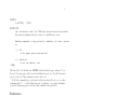
$ suplane | suxwigb title="suplane test pattern"
label1="time (s)" label2="trace number" &
^ Here the command is broken across a line
so it will fit this page of this book.
On your screen it would be typed as one
long line.
26
27
0
trace number
10
20
0.05
time (s)
0.10
0.15
0.20
0.25
suplane test pattern
Figure 2.1: The suplane test pattern.
27
30
28
to see a test pattern consisting of three intersecting lines in the form of seismic traces.
The data consist of seismic traces with only single values that are nonzero. This is
variable area display in which each place where the trace is positive valued is shaded
black. See Figure 2.1.
Equivalently, you should see the same output by typing
$ suplane > junk.su
$ suxwigb < junk.su
title="suplane test pattern"
label1="time (s)" label2="trace number" &
Finally, we often need to have graphical output that can be imported into documents.
In SU we have graphics programs that write output in the PostScript language
$ supswigb < junk.su title="suplane test pattern"
label1="time (s)" label2="trace number" > suplane.eps
2.1
Pipe |, redirect in < , redirect out >, and run
in background &
In the commands in the last section we used three symbols that allow files and programs
to send data to each other and to send data between programs. The vertical bar | is
called a “pipe” on all Unix-like systems. Output sent to standard out may be piped from
one program to another program as was done in the example of
$ suplane | suxwigb
&
which, in English may be translated as ”run suplane (pipe output to the program)
suxwigb where the & says (run all commands on this line in background).” The pipe
| is a memory buffer with a “read from standard input” for an input and a “write to
standard output” for an output. You can think of this as a kind of plumbing. A stream
of data, much like a stream of water is flowing from the program suplane to the program
suxwigb.
The “greater than” sign > is called “redirect out” and
$ suplane > junk.su
says ”run suplane (writing output to the file) junk.su. The > is a buffer which reads
from standard input and writes to the file whose name is supplied to the right of the
symbol. Think of this as data pouring out of the program suplane into the file junk.su.
The “lest than” sign < is called “redirect in” and
$ suxwigb < junk.su
&
says ”run suxwigb (reading the input from the file ) junk.su (run in background).
• | = pipe from program to program
28
29
a)
0
10
trace number
20
b)
30
10
0
trace number
20
30
20
0.05
40
time (s)
Freq. Hz
0.10
0.15
60
80
0.20
100
120
0.25
suplane test pattern
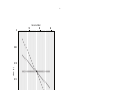
Figure 2.2: a) The suplane test pattern. b) the Fourier transform (time to frequency)
of the suplane test pattern via suspecfx.
• > = write data from program to file (redirect out)
• < = read data from file to program (redirect in)
• & = run program in background
2.2
Stringing commands together
We may string together programs via pipes (|), and input and output via redirects (>)
and (<). An example is to use the program suspecfx to look at the amplitude spectrum
of the traces in data made with suplane:
$ suplane | suspecfx | suxwigb
&
--make suplane data, find
the amplitude spectrum,
plot as wiggle traces
Equivalently, we may do
$ suplane > junk.su
$ suspecfx < junk.su > junk1.su
$ suxwigb < junk1.su
--make suplane data, write to a file.
--find the amplitude spectrum, write to
a file.
-- view the output as wiggle traces.
&
This does exactly the same thing, in terms of final output as the previous example,
with the exception that here, two files have been created. See Figure 2.2.
29
30
2.2.1
Questions for discussion
• What is the Fourier transform of a function?
• What is an amplitude spectrum?
• Why do the plots of the amplitude spectrum in Figure 2.2 appear as they do?
2.3
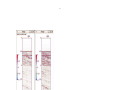
Unix Quick Reference Cards
The two figures, Fig 2.3 and Fig 2.4 are a Quick Reference cards for some Unix commands
References
Sobell, M. (2010), “A practical guide to Linux commands, editors, and shell programming” Pearson Education Inc., Boston, MA.
30
31
Figure 2.3: UNIX Quick Reference card p1. From the University References
31
32
Figure 2.4: UNIX Quick Reference card p2.
32
Chapter 3
Lab Activity #2 - viewing data
Just as scratch paper is paper that you use temporarily without the plan of saving for
the long term, a “scratch directory” is temporary working space, which is not backed up
and which may be arbitrarily cleared by the system administrator. Each computer in
this lab has a directory called /scratch that is provided as a temporary workspace for
users. It is in this location that you will be working with data. Create your own scratch
directory via:
$ mkdir /gpfc/yourusername
Here “yourusername” is the actual username that you are designated as on this system.
Please feel free to ask for help as you need it.
The /gpfc directory may reside physically on the computer where you are sitting, or
it may be remotely mounted. In computer environements where the directory is locally
on the a given computer, you will have to keep working on the same system. If you
change computers, you will have to transfer the items from your personal scratch area to
that new machine. In labs where the directory is remotely mounted, you may work on
any machine that has the directory mounted.
Remember: /scratch directories are not backed up. If you want to save materials
permanently, it is a good idea to make use of a USB storage device.
3.0.1
Data image examples
Three small datasets are provided. These are labeled “sonar.su,” “radar.su,” and “seismic.su” and are located in the directory
/data/cwpscratch/Data1/
We will pretend that these data examples are “data images,” which is to say these are
examples that require no further processing.
Do the following:
$ cd /gpfc/yourusername
(this takes you to /gpfc/yourusername)
33
34
^
This "$" represents the prompt at the beginning of the commandline.
Do not type the "$" when entering commands.
$
$
$
$
$
mkdir Temp1
(this creates the directory Temp1)
cd Temp1
(change working directory to Temp1)
cp /data/cwpscratch/Data1/sonar.su .
cp /data/cwpscratch/Data1/radar.su .
cp /data/cwpscratch/Data1/seismic.su .
^ This is a literal dot ".", which
means "the current directory"
$ ls
( should show the file sonar.su )
For the rest of this document, when you are directed to make “Temp” directories, it
will be assumed that you are putting these in your personal scratch directory.
3.1
Viewing an SU data file: Wiggle traces and
Image plots
Though we are assuming that the examples sonar.su, seismic.su, and radar.su are
finished products, our mode of presentation of these datasets may change the way we
view them entirely. Proper presentation can enhance features we want to see, suppress
parts of the data that we are less interested in, accentuate signal and suppress noise.
Improper presentation, on the other hand, can take turn the best images into something
that is totally useless.
3.1.1
Wiggle traces
A common mode of presentation of seismic data is the “wiggle trace.” Such a representation consists of representing the oscillations of the data as a graph of amplitude as a
function of time, with successive traces plotted side-by-side. Amplitudes of one polarity
(usually positive) are shaded black, where as negative amplitudes are not shaded. Be
aware that such presentation introduces a bias in the way we view the data, accentuating
the positive amplitudes. Furthermore, wiggle traces may make dipping structures appear
fatter than they actually are owing to the fact that a trace is a vertical slice through the
data.
In SU we may view a wiggle trace display of data via the program suxwigb. For
example, viewing the sonar.su data as wiggle traces is done by “redirecting in” the data
file into “suxwigb”
$ suxwigb < sonar.su
&
34
35
^ the ampersand (&) means "run in background"
so you get your commandline back
This should look horrible! The problem is that there are 584 wiggle traces, side by
side. Place the cursor on the plot and drag, while holding down the index finger mouse
button. This is called a “rubberband box.” Try grabbing a strip of the data of width less
than 100 traces, by placing the cursor at the top line of the plot, and holding the index
finger mouse button while dragging to the lower right. Zooming in this fashion will show
wiggles. The less on here is that you need a relatively low density of data on your print
medium for wiggle traces.
Place the mouse cursor on the plot, and type ”q” to kill the window.
Try the seismic.su and the radar.su data as wiggle traces via
$ suxwigb < seismic.su
$ suxwigb < radar.su
&
&
In each case, zoom in on the data until you are able to see the oscillations of the data.
3.1.2
Image plots
The seismic data may be thought of as an array of floating point numerical values, each
representing a seismic amplitude at a specific (t, x) location. A plot consisting of an array
of gray or color dots, with each gray level or color representing the respective value is
called an “image” plot.
If we view An alternative is an image plot:
$ suximage < sonar.su
&
This should look better. We usually use image plots for datasets of more than 50 traces.
We use wiggle traces for smaller datasets.
3.2
Greyscale
There are only 256 shades of gray available in this plot. If a single point in the dataset
makes a large spike, then it is possible that most of the 256 shades are used up by that
one amplitude. Therefore scaling amplitudes is often necessary. The simplest processing
of the data is to amplitude truncate (“clip”) the data. (The term “clip” refers to old
time strip chart records, which when amplitudes were too large appeared if someone had
taken scissors and clipped of the tops of the sinusoids of the oscillations.) Try:
$ suximage < sonar.su perc=99
&
$ suximage < sonar.su perc=99 legend=1
The perc=99 passes only those items of the 99th percentile and below in amplitude. (You
may need to look up “percentile” on the Internet.) In other words, it “clips” (amplitude
truncates) the data to remove the top 1 per cent of amplitudes. Try different values of
”perc” to see what this does.
35
36
0
200
400
0.05
0.10
0.15
0.20
0.25
Figure 3.1: Image of sonar.su data (no perc). Only the largest amplitudes are visible.
36
37
0
200
400
0.05
0.10
0.15
0.20
0.25
Figure 3.2: Image of sonar.su data with perc=99. Clipping the top 1 percentile of
amplitudes brings up the lower amplitude amplitudes of the plot.
37
38
3.3
Legend ; making grayscale values scientifically
meaningful
To be scientifically useful, which is to say “quantitative” we need to be able to translate
shades of gray into numerical values. This is done via a gray scale, or ”legend”. A
“legend” is a scale or other device that allows us to see the meanings of the graphical
convention used on a plot. Try:
$ suximage < sonar.su
legend=1
&
This will show a grayscale bar.
There are a number of colorscales available. Place the mouse cursor on the plot and
press “h” you will see that further pressings of “h” will re plot the data in a different
colorscale. Now press “r” a few times. The “h” scales are scales in “hue” and the “r”
scales are in red-green-blue (rgb). It is important to see that the brightest part of each
scale is chosen to emphasize a different amplitude.
With colormapping some parts of the plot may be emphasized at the expense of other
parts. The issue of colormaps often is one of selecting the location of the “bright part”
of the colorbar, versus darker colors. Even perfectly processed data may be rendered
uninterpretable by a poor selection of colormapping. This effect may be seen in Figure 3.4.
Repeat the previous, this time clipping by percentile
$ suximage < sonar.su
legend=1
perc=99
&
The ease at which colorscales are defined, and the fact that there are no real standards
on colorscales, mean that effectively every color plot you encounter requires a colorscale
for you to be able to know what the values mean. Furthermore, some colors ranges are
brighter than others. By moving the bright color to a different part of the amplitude
range, you can totally change the image. This is a source of richness of display, but it is
also a potential source of trouble, if the proper balance of color is not chosen.
3.4
Display balancing and display gaining
A common data amplitude balancing is to balance the colorscale on the median values
in the data. The “median” is the middle value, meaning that half the values are larger
than the median value and half the data are less than the median value. Thus, the traces
are normalized by this middle value.
Another possibility is to scale traces by dividing by some constant value. For example
dividing each trace by the square root of the average of the sum of the square of its values
(RMS).
Type these commands to see that in SU:
$ sunormalize norm=balmed < sonar.su | suximage legend=1
$ sunormalize norm=balmed < sonar.su | suximage legend=1 perc=99
38
39
0
200
400
0.05
4
2
0.10
0 0.15
-2
-4
0.20
0.25
Figure 3.3: Image of sonar.su data with perc=99 and legend=1.
39
40
Figure 3.4: Comparison of the default, hsv0, hsv2, and hsv7 colormaps. Rendering these
plots in grayscales emphasizes the location of the bright spot in the colorbar.
40
41
0
200
400
0.05
4
2
0.10
0 0.15
-2
-4
0.20
0.25
Figure 3.5: Image of sonar.su data with perc=99 and legend=1.
41
42
You may find perc=99 to be useful. You may find that you have to apply an “RMS”
balancing to make the data look a bit more uniform
$ sunormalize norm=balmed < sonar.su |
sunormalize norm=rms |
$ sunormalize norm=balmed < sonar.su |
sunormalize norm=rms |
suximage legend=1
suximage legend=1 perc=99
Again, these commands are written as one long line, and are broken here to fit on the
page. You may zoom in on regions of the plot you find interesting.
If you put both the median normalized and simple perc=99 files on the screen sideby-side, there are differences, but these may not be striking differences. The program
suximage has a feature that the user may change colormaps by pressing the “h” key
or the “r” key. Try this and you will see that the selection of the colormap can make
a considerable difference in the appearance of the image. Even with the same data, the
colormap.
For example in Figure 3.7 we see the result of applying median balancing. We might
consider applying sunormalize directly to the seismic data
$ suximage < seismic.su wbox=250 hbox=600 cmap=hsv4 clip=3 title="no median" &
compared with applying the median balancing
$ sunormalize norm=balmed < seismic.su |
suximage wbox=250 hbox=600
cmap=hsv4 clip=3 title="median filtering" &
This result looks bizarre because the traces individually have different median values and
consequently have different ranges of amplitudes. An improved picture may be obtained
by applying an RMS normalization to the traces after they have been median filtered
via,
$ sunormalize norm=balmed < seismic.su | sunormalize norm=rms |
suximage wbox=250 hbox=600
cmap=hsv4 clip=3 title="median filtering" &
In each of these examples, the line is broken to fit on the page. When you type this, the
pipe | follows immediately after the seismic.su.
There are other possibilities. We may consider simply normalizing the data by the
maximum or minimum value, or by some other constant. Furthermore, we have the
question of whether the process be applied trace by trace, or over the whole panel of
data.
42
43
0
200
400
0.05
3
2 0.10
1
0 0.15
-1
-2
-3
0.20
0.25
Figure 3.6: Image of sonar.su data with median balancing and perc=99
43
44
Figure 3.7: Comparison of seismic.su median-normalized, with the same data with no
median balancing. Amplitudes are clipped to 3.0 in each case. Notice that there are
features visible on the plot without median balancing that cannot be seen on the median
normalized data.
44
45
3.5
Homework problem #1 - Due dates Thursday 3
Sept 2015 and Tuesday 8 September 2015
Repeat display gaining experiments of the previous section with “radar.su” and “seismic.su” to see what median balancing, and setting perc=... does to these data.
• Capture representative plots with axes properly labeled. You can use the Linux
screen capture feature, or find another way to capture plots into a file, (such as
by using supsimage to make PostScript plots) Feel free to use different values of
perc and different colormaps than were used in the previous examples. Is median
filtering better? Is it worse? Can you simply change the clip value and get a better
picture?
The OpenOffice (or LibreOffice) Word wordprocessing program is an easy program
to use for this.
• Prepare a report of your results. The report should consist of:
– Your plots (you are telling a story, show only images are relevant to your
story)
– a short paragraph describing what you saw. Think of it as a figure caption.
– a listing of the actual commandlines that you ran to get the plots.
– Not more than 3 pages total!
– Make sure that your name, the due date, and the assignment number are at
the top of the first page.
• Save your report in the form of a PDF file, and email to [email protected]
3.6
Concluding Remarks
There are many ways of presenting data. Two of the most important questions that
a scientist can ask when seeing a plot are ”What is the meaning of the colorscale or
grayscale of a plot?” and ”What normalization or balancing has been applied to the data
before the plot?” The answers to these questions may be as important as the answer to
the question ”What processing has been applied to these data?”
3.6.1
What do the numbers mean?
The scale divisions seen on the plots in this chapter that have been obtained by running
suximage with legend=1 show numerical values, values that are changed when we
apply display gain. Ultimately, these numbers relate to the voltage recorded from a
transducer (a geophone, hydrophone, or accelerometer). While in theory we should be
able to extract information about the size of the ground displacement in, say micrometers,
45
46
or the pressure field strength in, say megapascals there is little reason to do this. Owing
to detector and source coupling issues, and the fact that data must be gathered quickly,
we really are only interested in relative values.
References
Stockwell, Jr. J. W. and J. K. Cohen (2008) The new SU users manual, available from
http:cwp.mines.edu/cwpcodes
46