Download GPGN 461/561 Lab Fall 2011 - Center for Wave Phenomena

Geophysical Image Processing with Seismic Unix:
GPGN 461/561 Lab
Fall 2011
Instructor: John Stockwell
Research Associate
Center for Wave Phenomena
c
copyright: John W. Stockwell, Jr. °2009,2010,2011
all rights reserved
License: You may download this document for educational
purposes and personal use, only, but not for
republication.
September 1, 2011
Contents
1 Seismic Processing Lab- Preliminary issues
1.1 Motivation for the lab . . . . . . . . . . . .
1.2 Unix and Unix-like operating systems . . . .
1.2.1 Steep learning curve . . . . . . . . .
1.3 Logging in . . . . . . . . . . . . . . . . . . .
1.4 What is a Shell? . . . . . . . . . . . . . . . .
1.5 The working environment . . . . . . . . . .
1.6 Setting the working environment . . . . . .
1.7 Choice of editor . . . . . . . . . . . . . . . .
1.8 The Unix directory structure . . . . . . . . .
1.9 Scratch and Data directories . . . . . . . . .
1.10 Shell environment variables and path . . . .
1.10.1 The path or PATH . . . . . . . . . .
1.10.2 The CWPROOT variable . . . . . .
1.11 Shell configuration files . . . . . . . . . . . .
1.12 Setting up the working environment . . . . .
1.12.1 The CSH-family . . . . . . . . . . . .
1.12.2 The SH-family . . . . . . . . . . . .
1.13 Unix help mechanism- Unix man pages . . .
.
.
.
.
.
.
.
.
.
.
.
.
.
.
.
.
.
.
2 Lab Activity #1 - Getting started with Unix
2.1 Pipe |, redirect in < , redirect out >, and run
2.2 Stringing commands together . . . . . . . . .
2.2.1 Questions for discussion . . . . . . . .
2.3 Unix Quick Reference Cards . . . . . . . . . .
.
.
.
.
.
.
.
.
.
.
.
.
.
.
.
.
.
.
.
.
.
.
.
.
.
.
.
.
.
.
.
.
.
.
.
.
.
.
.
.
.
.
.
.
.
.
.
.
.
.
.
.
.
.
.
.
.
.
.
.
.
.
.
.
.
.
.
.
.
.
.
.
.
.
.
.
.
.
.
.
.
.
.
.
.
.
.
.
.
.
.
.
.
.
.
.
.
.
.
.
.
.
.
.
.
.
.
.
.
.
.
.
.
.
.
.
.
.
.
.
.
.
.
.
.
.
.
.
.
.
.
.
.
.
.
.
.
.
.
.
.
.
.
.
.
.
.
.
.
.
.
.
.
.
.
.
.
.
.
.
.
.
and SU
in background &
. . . . . . . . . .
. . . . . . . . . .
. . . . . . . . . .
3 Lab Activity #2 - viewing data
3.0.1 Data image examples . . . . . . . . . . . . . . . . .
3.1 Viewing an SU data file: Wiggle traces and Image plots . .
3.1.1 Wiggle traces . . . . . . . . . . . . . . . . . . . . .
3.1.2 Image plots . . . . . . . . . . . . . . . . . . . . . .
3.2 Greyscale . . . . . . . . . . . . . . . . . . . . . . . . . . .
3.3 Legend ; making grayscale values scientifically meaningful .
3.4 Normalization: Median balancing . . . . . . . . . . . . . .
1
.
.
.
.
.
.
.
.
.
.
.
.
.
.
.
.
.
.
.
.
.
.
.
.
.
.
.
.
.
.
.
.
.
.
.
.
.
.
.
.
.
.
.
.
.
.
.
.
.
.
.
.
.
.
.
.
.
.
.
.
.
.
.
.
.
.
.
.
.
.
.
.
.
.
.
.
.
.
.
.
.
.
.
.
.
.
.
.
.
.
.
.
.
.
.
.
.
.
.
.
.
.
.
.
.
.
.
.
.
.
.
.
.
.
.
.
.
.
.
.
.
.
.
.
.
.
.
.
.
.
.
.
.
.
.
.
.
.
.
.
.
.
.
.
.
.
.
.
.
.
.
.
.
.
.
.
.
.
.
.
.
.
.
.
.
.
.
.
.
.
.
.
.
6
6
7
7
7
8
8
9
9
10
13
14
15
15
15
16
16
17
17
.
.
.
.
19
21
22
23
23
.
.
.
.
.
.
.
26
26
27
27
28
28
31
31
3.5
3.6
Homework problem #1 - Due Thursday 1 Sept 2011 . . . . . . . . . . . .
Concluding Remarks . . . . . . . . . . . . . . . . . . . . . . . . . . . . .
3.6.1 What do the numbers mean? . . . . . . . . . . . . . . . . . . . .
4 Help features in Seismic Unix
4.1 The selfdoc . . . . . . . . . . . . . . . . . . . . . . . .
4.2 Finding the names of programs with: suname . . . . .
4.3 Lab Activity #3 - Exploring the trace header structure
4.3.1 What are the trace header fields-sukeyword?
4.4 Concluding Remarks . . . . . . . . . . . . . . . . . . .
5 Lab
5.1
5.2
5.3
5.4
5.5
5.6
5.7
5.8
.
.
.
.
.
.
.
.
.
.
.
.
.
.
.
.
.
.
.
.
.
.
.
.
.
.
.
.
.
.
.
.
.
.
.
.
.
.
.
.
.
.
.
.
.
.
.
.
.
.
Activity #4 - Migration/Imaging as depth conversion
Imaging as the solution to an inverse problem . . . . . . . . . . . . . . .
Inverse scattering imaging as time-to-depth conversion . . . . . . . . . .
Time-to-depth with suttoz ; depth-to-time with suztot . . . . . . . . .
Time to depth conversion of a test pattern . . . . . . . . . . . . . . . . .
5.4.1 How time-depth and depth-time conversion works . . . . . . . . .
Sonar and Radar, bad header values and incomplete information . . . . .
The sonar data . . . . . . . . . . . . . . . . . . . . . . . . . . . . . . . .
Homework Problem - #2 - Time-to-depth conversion of the sonar.su and
the radar.su data. Due Thursday 8 Sept 2011 . . . . . . . . . . . . . . .
Concluding Remarks . . . . . . . . . . . . . . . . . . . . . . . . . . . . .
6 Zero-offset (aka poststack) migration
6.1 Migration as reverse time propagation. . . . . . . .
6.2 Lab Activity #5 - Hagedoorn’s graphical migration
6.3 Migration as a Diffraction stack . . . . . . . . . . .
6.4 Migration as a mathematical mapping . . . . . . .
6.5 Concluding Remarks . . . . . . . . . . . . . . . . .
2
.
.
.
.
.
.
.
.
.
.
.
.
.
.
.
.
.
.
.
.
.
.
.
.
.
.
.
.
.
.
.
.
.
.
.
.
.
.
.
.
.
.
.
.
.
.
.
.
.
.
.
.
.
.
.
.
.
.
.
.
36
38
38
39
39
40
42
42
52
53
53
54
55
55
59
60
60
62
62
63
65
67
71
72
73
List of Figures
1.1
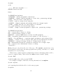
A quick reference for the vi editor. . . . . . . . . . . . . . . . . . . . . .
11
2.1
2.2
The suplane test pattern. . . . . . . . . . . . . . . . . . . . . . . . .
a) The suplane test pattern. b) the Fourier transform (time to frequency)
of the suplane test pattern via suspecfx. . . . . . . . . . . . . . . . . .
UNIX Quick Reference card p1. From the University References . . . . .
UNIX Quick Reference card p2. . . . . . . . . . . . . . . . . . . . . . .
20
2.3
2.4
3.1
3.2
3.3
3.4
3.5
3.6
3.7
5.1
5.2
Image of sonar.su data (no perc). Only the largest amplitudes are visible.
Image of sonar.su data with perc=99. Clipping the top 1 percentile of
amplitudes brings up the lower amplitude amplitudes of the plot. . . . .
Image of sonar.su data with perc=99 and legend=1. . . . . . . . . . .
Comparison of the default, hsv0, hsv2, and hsv7 colormaps. Rendering
these plots in grayscales emphasizes the location of the bright spot in the
colorbar. . . . . . . . . . . . . . . . . . . . . . . . . . . . . . . . . . . . .
Image of sonar.su data with perc=99 and legend=1. . . . . . . . . . .
Image of sonar.su data with median normalization and perc=99 . . . .
Comparison of seismic.su median-normalized, with the same data with
no median normalization. Amplitudes are clipped to 3.0 in each case. Note
that there are features visible on the plot without median normalization
that cannot be seen on the median normalized data. . . . . . . . . . . .
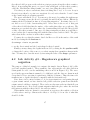
Cartoon showing the simple shifting of time to depth. The spatial coordinates x do not change in the transformation, only the time scale t is
stretched to the depth scale z. Note that vertical relief looks greater in a
depth section as compared with a time section. . . . . . . . . . . . . . .
a) Test pattern. b) Test pattern corrected from time to depth. c) Test
pattern corrected back from depth to time section. Note that the curvature
seen depth section indicates a non piecewise-constant v(t). Note that the
reconstructed time section has waveforms that are distorted by repeated
sinc interpolation. The sinc interpolation applied in the depth-to-time
calculation has not had an anti-alias filter applied. . . . . . . . . . . . .
3
22
24
25
29
30
32
33
34
35
37
54
56
5.3
6.1
6.2
6.3
6.4
6.5
6.6
6.7
6.8
6.9
a) Cartoon showing an idealized well log. b) Plot of a real well log. A
real well log is not well represented by piecewise constant layers. c) The
third plot is a linearly interpolated velocity profile following the example
in the text. This approximation is a better first-order approximation of a
real well log. . . . . . . . . . . . . . . . . . . . . . . . . . . . . . . . . .
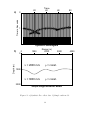
a) Synthetic Zero offset data. b) Simple earth model. . . . . . . . . . . .
The Hagedoorn method applied to the arrivals on a single seismic trace. .
Hagedoorn’s method applied to the simple data of Fig 6.1. Here circles,
each centered at time t = 0 on a specific trace, pass through the maximum
amplitudes on each arrival on each trace. The circle represents the locus
of possible reflection points in (x, z) where the signal in time could have
originated. . . . . . . . . . . . . . . . . . . . . . . . . . . . . . . . . . .
The dashed line is the interpreted reflector taken to be the envelope of the
circles. . . . . . . . . . . . . . . . . . . . . . . . . . . . . . . . . . . . .
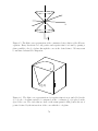
The light cone representation of the constant-velocity solution of the 2D
wave equation. Every wavefront for both positive and negative time t is
found by passing a plane parallel to the (x, z)-plane through the cone at
the desired time t. We may want to run time backwards for migration. .
The light cone representation for negative times is now embedded in the
(x, z, t)-cube. A seismic arrival to be migrated at the coordinates (ξ, τ ) is
placed at the apex of the cone. The circle that we draw on the seismogram
for that point is the set of points obtained by the intersection of the cone
with the t = 0-plane. . . . . . . . . . . . . . . . . . . . . . . . . . . . . .
Hagedoorn’s method of graphical migration applied to the diffraction from
a point scatterer. Only a few of the Hagedoorn circles are drawn, here, but
the reader should be aware that any Hagedoorn circle through a diffraction
event will intersect the apex of the diffraction hyperbola. . . . . . . . . .
The light cone for a point scatterer at (x, z). By classical geometry, a
vertical slice through the cone in (x, t) (the z = 0 plane where we record
our data) is a hyperbola. . . . . . . . . . . . . . . . . . . . . . . . . . . .
Cartoon showing the relationship between types of migration. a) shows
a point in (ξ, τ ), b) the impulse response of the migration operation in
(x, z), c) shows a diffraction, d) the diffraction stack as the output point
(x, z). . . . . . . . . . . . . . . . . . . . . . . . . . . . . . . . . . . . . .
4
57
64
68
68
69
70
70
71
72
73
Preface
I started writing these notes in 2005 to aid in the teaching of a seismic processing lab
that is part of the courses Seismic Processing GPGN561 and Advanced Seismic Methods
GPGN452 (later GPGN461) in the Department of Geophysics, Colorado School of Mines,
Golden, CO.
In October of 2005, Geophysics Department chairman Terry Young, asked me if I
would be willing to help teach the Seismic Processing Lab. This was the year following
Ken Larner’s retirement. Terry was teaching the lecture, but decided that the students
should have a practical problem to work on. The choice was between data shot in the
Geophysics Field Camp, the previous summer, or the Viking Graben dataset, which
Terry had brought with him from his time at Carnegie Mellon University. We chose
the latter, and decided that the students should produce as their final project, a poster
presentation similar to those seen at the SEG annual meeting. Terry seemed to think
that we could just hand the students the SU User’s Manual, and the data, and let them
have at it. I felt that more needed to be done to instruct students in the subject of
seismic processing, while simultaneously introducing them to the Unix operating system,
shell language programming, and of course Seismic Unx.
In the years that have elapsed my understanding of the subject of seismic processing
has continued to grow, and in each successive semester, I have gathered more examples,
and figured out how to apply more types of processing techniques to the data.
My vision of the material is that we are replicating the seismic processors’ base experience, such as a professional would have obtained in the petroleum industry in the
late 1970s. The idea is not to train students in a particular routine of processing, but
to teach them how to think like geophysicists. Because seismic processing techniques
are not exclusively used on petroleum industry data, the notion of “geophysical image
processing” rather than simply “seismic” processing is conveyed.
5
Chapter 1
Seismic Processing Lab- Preliminary
issues
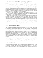
1.1
Motivation for the lab
In the lecture portion of the course GPGN452/561 (now GPGN461/561) (Advanced Seismic Methods/Seismic Processing) the student is given a word, picture, and chalkboard
introduction of the process of seismic data acquisition and the application of a myriad of
processing steps for converting raw seismic data into a scientifically useful picture of the
earth’s subsurface.
This lab is designed to provide students with a practical hands-on experience in the
reality of applying seismic processing techniques to synthetic and real data. The course,
however, is not a “training course in seismic processing,” as one might get in an industrial
setting. Rather than training a student to use a particular collection of software tools,
we believe that it is better that the student cultivate a broader understanding of the
subject of seismic processing. We seek also to help students develop some practical skills
that will serve them in a general way, even if they do not go into the field of oil and gas
exploration and development.
Consequently, we make use of freely available open-source software (the Seismic Unix
package) running on small-scale hardware (Linux-based PCs). Students are also encouraged to install the SU software on their own personal (Linux or Mac) PCs, so that they
may work (and play) with the data and with the codes at their leisure.
Given the limited scale of our available hardware and time, our goal is modest, to
introduce students to seismic data processing through a 2D single-component processing
application.
The intended range of experience is approximately that which a seismic processor
of the late 1970s would have experienced on a vastly slower, more expensive, and more
difficult to use processing platform.
6
1.2
Unix and Unix-like operating systems
The Unix operating system (as well as any other Unix-like operating system, which
includes the various forms of Linux, UBUNTU, Free BSD Unix, and Mac OS X) is
commonly used in the exploration seismic community. Consequently, learning aspects
this operating system is time well spent. Many users may have grown up with a “point
and click” environment where a given program is run via a graphical user interface (GUI)
featuring menus and assorted windows. Certainly there are such software applications in
the world of commercial seismic processing, but none of these are inexpensive, and none
give the user access to the source code of the application.
There is also an “expert user” level of work where such GUI-driven tools do not
exist, however, and programs are run from the commandline of a terminal window or are
executed as part of a processing sequence in shell script.
In this course we will use the open source CWP/SU:Seismic Unix (called simply Seismic Unix or SU) seismic processing and research environment. This software collection
was developed largely at the Colorado School of Mines (CSM) at the Center for Wave
Phenomena (CWP), with contributions from users all around the world. The SU software package is designed to run under any Unix or Unix-like operating system, and is
available as full source code. Students are free to install Linux and SU on their PCs (or
use Unix-like alternatives) and thus have the software as well as the data provided for
the course for home use, during, and beyond the time of the course.
1.2.1
Steep learning curve
The disadvantage that most beginning Unix users face is a steep learning curve owing
to the myriad commands that comprise Unix and other Unix-like operating systems.
The advantages of software portability and flexibility of applications, as well as superior
networking capability, however, makes Unix more attractive to industry than Microsoftbased systems for these expert level applications. While a user in an industrial environment may have a Microsoft-based PC on his or her desk, the more computationally
intensive processing work is done on a Unix-based system. The largest of these are
clusters composed of multi-core, multiprocessor PC systems. It is not uncommon these
days for such systems to have several thousand “cores,” which is to say subprocessors,
available.
Because a course in seismic processing is of broad interest and may draw students
with varied backgrounds and varied familiarity with computing systems, we begin with
the basics. The reader familiar with these topics may skip to the next chapter.
1.3
Logging in
As with most computer systems, there is a prompt, usually containing the word ”login”
or the word ”username” that indicates the place where the user logs in. The user is
then prompted for a password. Once on the system, the user either has a windowed user
7
interface as the default, or initiates such an interface with a command, such as startx
in Linux.
1.4
What is a Shell?
Some of the difficult and confusing aspects of Unix and Unix-like operating systems are
encountered at the very beginning of using the system. The first of these is the notion of
a shell. Unix is an hierarchical operating system that runs a program called the kernel
that is is the heart of the operating system. Everything else consists of programs that are
run by the kernel and which give the user access to the kernel and thus to the hardware
of the machine.
The program that allows the user interfaces with the computer is called the “working
shell.” The basic level of shell on all Unix systems is called sh, the Bourne shell. Under
Linux-based systems, this shell is actually an open-source rewritten version called bash
(the Bourne again shell), but it has an alias that makes it appear to be the same as the
sh that is found on all other Unix and Unix-like systems.
The common working shell environment that a user is usually set up to login in under
may be csh (the C-shell), tcsh (the T-shell, which is a non proprietary version of csh,
ksh (the Korn shell, which is proprietary), zsh which is an open source version of Korn
shell, or bash, which is an open source version of the Bourne shell.
The user has access to an application called terminal in the graphical user environment, that when launched (usually by double clicking) invokes a window called a terminal
window. (The word“terminal” harks back to an earlier day, when a physical device called
a terminal consisting of a screen and keyboard (but no mouse) constituted the users’
interface to the computer.) It is at the prompt on the terminal window that the user has
access to a commandline where Unix commands are typed.
Most “commands” on Unix-like systems are not built in commands in the shell, but
are actually programs that are run under the users’ working shell environment. The shell
commandline prompt is asking the user to input the name of an executable program.
1.5
The working environment
In the Unix world all filenames, program names, shells, and directory names, as well as
passwords are case sensitive in their input, so please be careful in running the examples
that follow.
If the user types:
$ cd
^
(don’t type the dollar sign)
<--- change directory with no argument
takes the user to his/her home
directory
In these notes, the $ symbol will represent the commandline prompt. The user does not
type this $. Because there are a large variety of possible prompt characters, or strings of
8
characters that people use for the propmt, we show here only the dollar sign $ as a generic
commmandline prompt. On your system it might be a %, a >, or some combination of
these with the computer name and or the working directory and/or the commandline
number.
$ echo $SHELL
^
type this dollar sign
<--- returns the value of the users’
working shell environment
The command echo $SHELL tells your working shell to return the value that denotes
your working shell environment. In English this command might be translated as “print
the value of the variable SHELL”. In this context the dollar sign $ in front of SHELL
should be translated as “value of”.
Common possible shells are
/bin/sh
/bin/bash
/bin/ksh
/bin/zsh
/bin/csh
/bin/tcsh
<--<--<--<--<--<---
the Bourne Shell
the Bourne again Shell
K-shell
Z-shell
C-shell
T-shell.
The environments sh, bash, ksh, and zsh are similar. We will call these the “sh-family.”
The environments csh and tcsh are similar to each other, but have many differences from
the sh-family. We refer to csh and tcsh as the csh-family.
1.6
Setting the working environment
Each of these programs have a specific syntax, which can be quite complicated. Each
is a language that allows the user to write programs called “shell scripts.” Thus Unixlike systems have scripting languages as their basic interface environment. This endows
Unix-like operating systems with vastly more flexibility and power than other operating
systems you may have encountered.
With more flexibility and power, there comes more complexity. It is possible to
perform many configuration changes and personalizations to your working environment,
which can enhance your user experience. For these notes we concentrate only on enough
of these to allow you to work effectively on the examples in the text.
1.7
Choice of editor
To edit files on a Unix-like system, the user must adopt an editor. The traditional Unix
editor is vi or one of its non-proprietary clones vim (vi-improved), gvim, or elvis. The
9
vi environment has a steep learning curve making it often unpopular among beginners.
If a person is envisioning working on Unix-like systems a lot, then taking the time to
learn vi is also time well spent. The vi editor is the only editor that is guaranteed to
be on all Unix-like systems. All other editors are third-party items that may have to be
added on some systems, sometimes with difficulty.
Similarly there is an editor called emacs that is popular among many users, largely
because it is possible to write programs in the LISP language and implement these
within emacs. There is a steep learning curve for this language, as well. There is often
substantial configuration required to get emacs working in the way the user desires.
A third editor is called pico, which comes with a mailer called “pine.” Pico is easy
to learn to use, fully menued, and runs in a terminal window.
The fourth class of editor consists of the “screen editors.” Popular screen editors
include xedit, nedit, and gedit. There is a windowed interfaced version of emacs called
xemacs that is similar to the first two editors. These are all easy to learn and to use.
Not all editors are the best to use. The user may find that invisible characters are
introduced by some editors, and that there may be issues regarding how wrapped lines
are handled that may cause problems for some applications. (More advanced issues such
as those which might be of interest to a Unix system administrator, narrow the field back
to vi.)
The choice of editor is often a highly personal one depending on what the user is
familiar with, or is trying to accomplish. Any of the above mentioned editors, or similar
third party editors likely are sufficient for the purposes of this course.
1.8
The Unix directory structure
As with other computing systems, data and programs are contained in “files” and “files”
are contained in “folders.” In Unix and all Unix-like environments “folders” are called
“directories.”
The structure of directories in Unix is that of an upside down tree, with its root at the
top, and its branches—subdirectories and the files they contain—extending downward.
The root directory is called “/” (pronounced “slash”).
While there exist graphical browsers on most Unix-like operating systems, it is more
efficient for users working on the commandline of a terminal windows to use a few simple
commands to view and navigate the contents of the directory structure. These commands
pwd (print working directory), ls (list contents), and cd (change directory).
Locating yourself on the system
If you type:
$ cd
$ pwd
$ ls
10
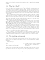
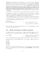
Vi Quick Reference
http://www.sfu.ca/~yzhang/linux
MOVEMENT
(lines - ends at <CR>; sentence - ends at puncuation-space; section - ends at <EOF>)
By Character
k
h
hjkl
l
j
By Line
nG
0, $
^ or _
+, -
to line n
first, last position on line
first non-whitespace char on line
first character on next, prev line
By Screen
^F, ^B
^D, ^U
^E, ^Y
L
z↵
↵
z.
z-
scroll foward, back one full screen
scroll forward, back half a screen
show one more line at bottom, top
go to the bottom of the screen
position line with cursor at top
position line with cursor at middle
position line with cursor at
Marking Position on Screen
mp
mark current position as p (a..z)
`p
move to mark position p
'p
move to first non-whitespace on line w/mark p
Miscellaneous Movement
fm
forward to character m
Fm
backward to character m
tm
forward to character before m
Tm
backward to character after m
w
move to next word (stops at puncuation)
W
move to next word (skips punctuation)
b
move to previous word (stops at punctuation)
B
move to previous word (skips punctuation)
e
end of word (puncuation not part of word)
E
end of word (punctuation part of word)
), (
next, previous sentence
]], [[ next, previous section
}, {
next, previous paragraph
%
goto matching parenthesis () {} []
EDITING TEXT
Entering Text
a
append after cursor
A or $a
append at end of line
i
insert before cursor
I or _i
insert at beginning of line
o
open line below cursor
O
open line above cursor
cm
change text (m is movement)
Cut, Copy, Paste (Working w/Buffers)
dm
delete (m is movement)
dd
delete line
D or d$
delete to end of line
x
delete char under cursor
X
delete char before cursor
ym
yank to buffer (m is movement)
yy or Y
yank to buffer current line
p
paste from buffer after cursor
P
paste from buffer before cursor
“bdd
cut line into named buffer b (a..z)
“bp
paste from named buffer b
Searching and Replacing
/w
search forward for w
?w
search backward for w
/w/+n search forward for w and move down n lines
n
repeat search (forward)
N
repeat search (backward)
:s/old/new
:s/old/new/g
:x,ys/old/new/g
:%s/old/new/g
:%s/old/new/gc
replace next occurence of old with new
replace all occurences on the line
replace all ocurrences from line x to y
replace all occurrences in file
same as above, with confirmation
Miscellaneous
n>m indent n lines (m is movement)
n<m un-indent left n lines (m is movement)
.
repeat last command
U
undo changes on current line
u
undo last command
J
join end of line with next line (at <cr>)
:rf
insert text from external file f
^G
show status
Figure 1.1: A quick reference for the vi editor.
11
You will see that your current working directory location, which is your called your “home
directory.” You should see something like
$ pwd
/home/yourusername
where “yourusername” is your username on the system. Other users likely have their
home directories in
/home
or something similar, depending on how your system administrator has set things up.
The command ls will show you the contents of your home directory, which may consist
of files or other subdirectories.
The codes for Seismic Unix are installed in some system directory path. We will
assume that all of the CWP/SU: Seismic Unix codes are located in
/usr/local/cwp
This denotes a directory “cwp,” which is the sub directory of a directory called “local,”
which is in turn a directory of the directory “usr,” that itself is a sub directory of slash.
It is worth wile for the user to spend some time learning the layout of his or her
directories. There is a command called
$ df
which shows the hardware devices that constitute the available storage on the users’
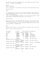
machine. A typical output from typing “df”
Filesystem
1K-blocks
Used Available Use% Mounted on
/dev/sda1
295101892 45219392 234892216 17% /
none
4070496
268
4070228
1% /dev
none
4075032
4988
4070044
1% /dev/shm
none
4075032
124
4074908
1% /var/run
none
4075032
0
4075032
0% /var/lock
none
4075032
0
4075032
0% /lib/init/rw
isengard.mines.edu:/usr/local/cwp
20314752
6037440 13228736 32% /usr/local/cwp
isengard.mines.edu:/usr/local/sedpak54
20314752
6037440 13228736 32% /usr/local/sedpak54
isengard.mines.edu:/u
206424768 50614912 145324096 26% /u
isengard.mines.edu:/data/cwpscratch
30963712
9732128 19658720 34% /cwpscratch
isengard.mines.edu:/data
103212320 19418464 78550976 20% /data
12
isengard.mines.edu:/scratch
396341312
199520 376008736
1% /scratch
the hardware devices on the far left column. Those whose names begin with “dev”
are hardware devices on the specific computer. The items that begin with a machine
name, in this case “isengard.mines.edu” exist physically on another machine (named
“isengard”), but are remotely mounted as to appear to be on this machine. The
second column from the left shows the total space on the device, the third column shows
the amount of space used, while the fourth shows the amount available, the fifth column
shows the usage as a percentage of space used. Finally the far right column shows the
directory where these devices are mounted.
In Unix devices are mounted in such a way that they appear to be files or directories.
Under Unix-like operating systems, the user sees only a directory tree, and not individual
hardware devices.
If you try editing files in some of these other directories you will find that you likely do
not have permission to read, write, or modify the contents of many those directories. Unix
is a multi-user environment, meaning that from an early day, the notion of protecting
users from each other and from themselves, as well as protecting the operating system
from the users has been a priority from day one.
In none of these examples have we used a browser, yet there are browsers available
on most Unix systems. There is no fundamental problem with using a browser, with
the exception that you have to take your hands off the keyboard to use the mouse. The
browser will not tell you where you are located within a terminal window. If you must
use a browser, use “column view” rather than “icon view” as we will have many levels of
nested directories to navigate.
1.9
Scratch and Data directories
Directories with names such “scratch” and “data” are often provided with user write
permission so that users may keep temporary files and data files out of their home directories. Like “scratch paper” a scratch directory is usually for temporary file storage, and
is not backed up. Indeed, on any computer system there may be “scratch” directories
that are not called by that name.
Also, such directories may be physically located on the specific machine were you are
seated and may not be visible on other machines. Because the redundancy of backups
require extra storage, most system administrators restrict the amount of backed up space
to a relatively small area of a computer system. To restrict user access, quotas may be
imposed that will prevent users from using so much space that a single user could fill up a
disk. However, in scratch areas there usually are no such restriction, so it is preferable to
work in these directories, and save only really important materials in your home directory.
Users should be aware, that administration of scratch directories may not be user
friendly. Using up all of the space on a partition may have dire consequences, in that the
13
administrator may simply remove items that are too big, or have a policy of removing
items that have not been accessed over a certain period of time. A system administrator may also set up an automated “grim file reaper” to automatically delete materials
that have not been accessed after a period of time. Because files are not always
automatically backed up, and because hardware failures are possible on any
system, it is a good idea for the user to purchase USB storage media and get
in the habit of making personal backups on a regular basis. A less hostile mode
of management is to institute quotas to prevent single users from hogging the available
scratch space.
You may see a scratch directory on any of the machines in your lab, but these are
different directories, each located on a different hard drive. This can lead to confusion
as a user may copy stuff into a scratch area on one day, and then work on a different
computer on a different day, thinking that their stuff has been removed.
The availability and use of scratch directories is important, because each user has a
quota that limits the amount of space that he or she may use in his/her home directory.
On systems where a scratch directory is provided, that also has write permission, the
user may create his/her personal work area via
$ cd /scratch
$ mkdir yourusername
<--- here "yourusername" is the
your user name on the system
Unless otherwise stated, this text will assume that you are conducting further operations
in your personal scratch work area.
1.10
Shell environment variables and path
The working shell is a program that has a configuration that gives the user access to
executable files on the system. Recall that echoing the value of the SHELL variable
$ echo $SHELL
<--- returns the value of the users’
working shell environment
tells you what shell program is your working shell environment. There are other environmental variables other than SHELL. Again, note that if this command returns one of
the values
/bin/sh
/bin/ksh
/bin/bash
/bin/zsh
then you are working in the SH-family and need to follow instructions for working with
that type of environment. If, on the other hand, the echo $SHELL command returns
one of the values
14
/bin/csh
/bin/tcsh
then you are working in the CSH-family and need to follow the alternate series of instructions given.
In the modern world of Linux, it is quite common for the default shell to be something
called binbash an open-source version of binsh.
1.10.1
The path or PATH
Another important variable is the “path” or “PATH”. The value path variable tells the
location that the working shell looks for executable files in. Usually, executables are
stored in a sub directory “bin” of some directory. Because there may be many software
packages installed on a system, there may be many such locations.
To find out what paths you can access, which is to say, which executables your shell
can see, type
$ echo $path
or
$ echo $PATH
The result will be a listing, separated by colons “:” of paths or by spaces “ ” to executable
programs.
1.10.2
The CWPROOT variable
The variable PATH is important, but SHELL and PATH are not the only possible environment variable. Often programmers will use an environment variable to give a users’
shell access to some attribute or information regarding a specific piece of software. This
is done because sometimes software packages are of restricted interest.
For SU the path CWPROOT is necessary for running the SU suite of programs. We
need to set this environment variable, and to put the suite of Seismic Unix programs on
the users’ path.
1.11
Shell configuration files
Because the users’ shell has as an attribute a natural programming language, many
configurations of the shell environment are possible. To find the configuration files for
your operating system, type
$ ls -a
<--- show directory listing of all
files and sub directories
<--- print working directory
$ pwd
then the user will see a number of files whose names begin with a dot ”.”.
15
1.12
Setting up the working environment
One of the most difficult and confusing aspects of working on Unix-like systems is encountered right at the beginning. This is the problem of setting up user’s personal
environment. There are two sets of instructions given here. One for the CSH-family of
shells and the other for the SH-family.
1.12.1
The CSH-family
Each of the shell types returned by $SHELL has a different configuration file. For the
csh-family (tcsh,csh), the configuration files are “.cshrc” and “.login”. To configure the
shell, edit the file .cshrc. Also, the “path” variable is lower case.
You will likely find a line beginning with
set path=(
with entries something like
set path=( /lib ~/bin /usr/bin/X11 /usr/local/bin /bin
/usr/bin . /usr/local/bin /usr/sbin )
Suppose that the Seismic Unix package is installed in the directory
/usr/local/cwp
on your system.
Then we would add one line above to set the “CWPROOT” environment variable.
And one line below to define the user’s “path”
setenv CWPROOT /usr/local/cwp
set path=( /lib ~/bin /usr/bin/X11 /usr/local/bin /bin
/usr/bin . /usr/local/bin /usr/sbin )
set path=( $path $CWPROOT/bin )
Save the file, and log out and log back in. You will need to log out completely from the
system, not just from particular terminal windows.
When you log back in, and pull up a terminal window, typing
$ echo $CWPROOT
will yield
/usr/local/cwp
16
and
$ echo $PATH
will yield
/lib /u/yourusername/bin /usr/bin/X11 /usr/local/bin /bin
/usr/bin . /usr/local/bin /usr/sbin /usr/local/cwp/bin
1.12.2
The SH-family
The process is similar for the SH-family of shells. The file of interest has a name of the
form “.profile,” .bashrc,” and the “.bash profile.” The “.bash profile” is read once by the
shell, but the “.bashrc” file is read everytime a window is opened or a shell is invoked.
Thus, what is set here influences the users complete environment. The default form of
this file may show a path line similar to
PATH=$PATH:$HOME/bin:.:/usr/local/bin
which should be edited to read
export CWPROOT=/usr/local/cwp
PATH=$PATH:$HOME/bin:.:/usr/local/bin:$CWPROOT/bin
The important part of the path is to add the
:$CWPROOT/bin
on the end of the PATH line, no matter what it says.
The user then logs out and logs back in for the changes to take effect. In each case,
the PATH and CWPROOT variables are necessary to be set for the users’ working shell
environment to find the executables of Seismic Unix.
1.13
Unix help mechanism- Unix man pages
Every program on a Unix or Unix-like system has a system manual page, called a man
page, that gives a terse description of its usage. For example, type:
$
$
$
$
$
$
man
man
man
man
man
man
ls
cd
df
sh
bash
csh
to see what the system says about these commands. For example:
17
$ man ls
LS(1)
User Commands
LS(1)
NAME
ls - list directory contents
SYNOPSIS
ls [OPTION]... [FILE]...
DESCRIPTION
List information about the FILEs (the current directory by default).
Sort entries alphabetically if none of -cftuvSUX nor --sort.
Mandatory arguments to long options are
too.
mandatory
for
short
options
-a, --all
do not ignore entries starting with .
-A, --almost-all
do not list implied . and ..
--MOREThe item at the bottom that says –MORE– indicates that the page continues. To see
the rest of the man page for ls is viewed by hitting the space bar. View the Unix man
page for each of the Unix commands you have used so far.
Most Unix commands have options such as the ls -a which allowed you to see files
beginning with dot “.” or ls -l which shows the “long listing” of programs. Remember
to view the Unix man pages of each new Unix command as it is presented.
18
Chapter 2
Lab Activity #1 - Getting started
with Unix and SU
Any program that has executable permissions and which appears on the users’ PATH
may be run by simply typing its name on the commandline. For example, if you have
set your path correctly, you should be able to do the following
$ suplane | suxwigb
&
^ this symbol, the ampersand, indicates that
the program is being run in background
^ the "pipe" symbol
The commandline itself is the interactive prompt that the shell program is providing so
that you can supply input. The proper input for a commandline is an executable file,
which may be a compiled program or a Unix shell script. The command prompt is saying,
”Type program name here.”
Try running this command with and without the ampersand &. If you run
$ suplane | suxwigb
The plot comes up, but you have to kill the plot window before you can get your commandline back, whereas
$ suplane | suxwigb
&
allows you to have the plot on the screen, and have the commandline.
To make the plot better we may add some axis labeling:
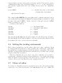
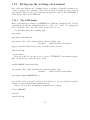
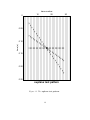
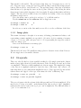
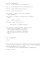
$ suplane | suxwigb title="suplane test pattern"
label1="time (s)" label2="trace number" &
^ Here the command is broken across a line
so it will fit this page of this book.
On your screen it would be typed as one
long line.
19
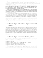
0
10
trace number
20
0.05
time (s)
0.10
0.15
0.20
0.25
suplane test pattern
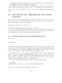
Figure 2.1: The suplane test pattern.
20
30
to see a test pattern consisting of three intersecting lines in the form of seismic traces.
The data consist of seismic traces with only single values that are nonzero. This is
variable area display in which each place where the trace is positive valued is shaded
black. See Figure 2.1.
Equivalently, you should see the same output by typing
$ suplane > junk.su
$ suxwigb < junk.su
title="suplane test pattern"
label1="time (s)" label2="trace number" &
Finally, we often need to have graphical output that can be imported into documents.
In SU we have graphics programs that write output in the PostScript language
$ supswigb < junk.su title="suplane test pattern"
label1="time (s)" label2="trace number" > suplane.eps
2.1
Pipe |, redirect in < , redirect out >, and run
in background &
In the commands in the last section we used three symbols that allow files and programs
to send data to each other and to send data between programs. The vertical bar | is
called a “pipe” on all Unix-like systems. Output sent to standard out may be piped from
one program to another program as was done in the example of
$ suplane | suxwigb
&
which, in English may be translated as ”run suplane (pipe output to the program)
suxwigb where the & says (run all commands on this line in background).” The pipe
| is a memory buffer with a “read from standard input” for an input and a “write to
standard output” for an output. You can think of this as a kind of plumbing. A stream
of data, much like a stream of water is flowing from the program suplane to the program
suxwigb.
The “greater than” sign > is called “redirect out” and
$ suplane > junk.su
says ”run suplane (writing output to the file) junk.su. The > is a buffer which reads
from standard input and writes to the file whose name is supplied to the right of the
symbol. Think of this as data pouring out of the program suplane into the file junk.su.
The “lest than” sign < is called “redirect in” and
$ suxwigb < junk.su
&
says ”run suxwigb (reading the input from the file ) junk.su (run in background).
• | = pipe from program to program
21
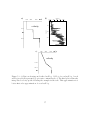
a)
0
10
trace number
20
b)
30
10
0
trace number
20
30
20
0.05
40
time (s)
Freq. Hz
0.10
60
0.15
80
0.20
100
120
0.25
suplane test pattern
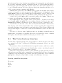
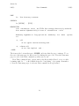
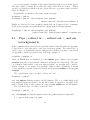
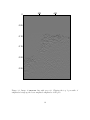
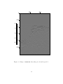
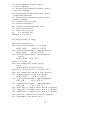
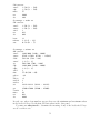
Figure 2.2: a) The suplane test pattern. b) the Fourier transform (time to frequency)
of the suplane test pattern via suspecfx.
• > = write data from program to file (redirect out)
• < = read data from file to program (redirect in)
• & = run program in background
2.2
Stringing commands together
We may string together programs via pipes (|), and input and output via redirects (>)
and (<). An example is to use the program suspecfx to look at the amplitude spectrum
of the traces in data made with suplane:
$ suplane | suspecfx | suxwigb
&
--make suplane data, find
the amplitude spectrum,
plot as wiggle traces
Equivalently, we may do
$ suplane > junk.su
$ suspecfx < junk.su > junk1.su
$ suxwigb < junk1.su
--make suplane data, write to a file.
--find the amplitude spectrum, write to
a file.
-- view the output as wiggle traces.
&
This does exactly the same thing, in terms of final output as the previous example,
with the exception that here, two files have been created. See Figure 2.2.
22
2.2.1
Questions for discussion
• What is the Fourier transform of a function?
• What is an amplitude spectrum?
• Why do the plots of the amplitude spectrum in Figure 2.2 appear as they do?
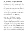
2.3
Unix Quick Reference Cards
The two figures, Fig 2.3 and Fig 2.4 are a Quick Reference cards for some Unix commands
23
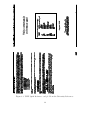
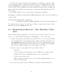
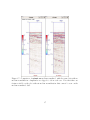
Figure 2.3: UNIX Quick Reference card p1. From the University References
24
Figure 2.4: UNIX Quick Reference card p2.
25
Chapter 3
Lab Activity #2 - viewing data
Just as scratch paper is paper that you use temporarily without the plan of saving for
the long term, a “scratch directory” is temporary working space, which is not backed up
and which may be arbitrarily cleared by the system administrator. Each computer in
this lab has a directory called /scratch that is provided as a temporary workspace for
users. It is in this location that you will be working with data. Create your own scratch
directory via:
$ mkdir /scratch/yourusername
Here “yourusername” is the actual username that you are designated as on this system.
Please feel free to ask for help as you need it.
The /scratch directory may reside physically on the computer where you are sitting,
or it may be remotely mounted. In computer environements where the directory is locally
on the a given computer, you will have to keep working on the same system. If you change
computers, you will have to transfer the items from your personal scratch area to that
new machine. In labs where the directory is remotely mounted, you may work on any
machine that has the directory mounted.
Remember: /scratch directories are not backed up. If you want to save materials
permanently, it is a good idea to make use of a USB storage device.
3.0.1
Data image examples
Three small datasets are provided. These are labeled “sonar.su,” “radar.su,” and “seismic.su” and are located in the directory
/cwpscratch/Data1/
We will pretend that these data examples are “data images,” which is to say these are
examples that require no further processing.
Do the following:
$ cd /scratch/yourusername
(this takes you to /scratch/yourusername)
26
^
This "$" represents the prompt at the beginning of the commandline.
Do not type the "$" when entering commands.
$
$
$
$
$
mkdir Temp1
(this creates the directory Temp1)
cd Temp1
(change working directory to Temp1)
cp /cwpscratch/Data1/sonar.su .
cp /cwpscratch/Data1/radar.su .
cp /cwpscratch/Data1/seismic.su .
^ This is a literal dot ".", which
means "the current directory"
$ ls
( should show the file sonar.su )
For the rest of this document, when you are directed to make “Temp” directories, it
will be assumed that you are putting these in your personal scratch directory.
3.1
Viewing an SU data file: Wiggle traces and
Image plots
Though we are assuming that the examples sonar.su, seismic.su, and radar.su are
finished products, our mode of presentation of these datasets may change the way we
view them entirely. Proper presentation can enhance features we want to see, suppress
parts of the data that we are less interested in, accentuate signal and suppress noise.
Improper presentation, on the other hand, can take turn the best images into something
that is totally useless.
3.1.1
Wiggle traces
A common mode of presentation of seismic data is the “wiggle trace.” Such a representation consists of representing the oscillations of the data as a graph of amplitude as a
function of time, with successive traces plotted side-by-side. Amplitudes of one polarity
(usually positive) are shaded black, where as negative amplitudes are not shaded. Note
that such presentation introduces a bias in the way we view the data, accentuating the
positive amplitudes. Furthermore, wiggle traces may make dipping structures appear
fatter than they actually are owing to the fact that a trace is a vertical slice through the
data.
In SU we may view a wiggle trace display of data via the program suxwigb. For
example, viewing the sonar.su data as wiggle traces is done by “redirecting in” the data
file into “suxwigb”
$ suxwigb < sonar.su
&
^ the ampersand (&) means "run in background"
27
This should look horrible! The problem is that there are 584 wiggle traces, side by
side. Place the cursor on the plot and drag, while holding down the index finger mouse
button. This is called a “rubberband box.” Try grabbing a strip of the data of width less
than 100 traces, by placing the cursor at the top line of the plot, and holding the index
finger mouse button while dragging to the lower right. Zooming in this fashion will show
wiggles. The less on here is that you need a relatively low density of data on your print
medium for wiggle traces.
Place the mouse cursor on the plot, and type ”q” to kill the window.
Try the seismic.su and the radar.su data as wiggle traces via
$ suxwigb < seismic.su
$ suxwigb < radar.su
&
&
In each case, zoom in on the data until you are able to see the oscillations of the data.
3.1.2
Image plots
The seismic data may be thought of as an array of floating point numerical values, each
representing a seismic amplitude at a specific (t, x) location. A plot consisting of an array
of gray or color dots, with each gray level or color representing the respective value is
called an “image” plot.
If we view An alternative is an image plot:
$ suximage < sonar.su
&
This should look better. We usually use image plots for datasets of more than 50 traces.
We use wiggle traces for smaller datasets.
3.2
Greyscale
There are only 256 shades of gray available in this plot. If a single point in the dataset
makes a large spike, then it is possible that most of the 256 shades are used up by that
one amplitude. Therefore scaling amplitudes is often necessary. The simplest processing
of the data is to amplitude truncate (“clip”) the data. (The term “clip” refers to old
time strip chart records, which when amplitudes were too large appeared if someone had
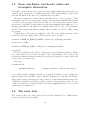
taken scissors and clipped of the tops of the sinusoids of the oscillations.) Try:
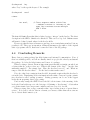
$ suximage < sonar.su perc=99
&
$ suximage < sonar.su perc=99 legend=1
The perc=99 passes only those items of the 99th percentile and below in amplitude. (You
may need to look up “percentile” on the Internet.) In other words, it “clips” (amplitude
truncates) the data to remove the top 1 per cent of amplitudes. Try different values of
”perc” to see what this does.
28
0
200
400
0.05
0.10
0.15
0.20
0.25
Figure 3.1: Image of sonar.su data (no perc). Only the largest amplitudes are visible.
29
0
200
400
0.05
0.10
0.15
0.20
0.25
Figure 3.2: Image of sonar.su data with perc=99. Clipping the top 1 percentile of
amplitudes brings up the lower amplitude amplitudes of the plot.
30
3.3
Legend ; making grayscale values scientifically
meaningful
To be scientifically useful, which is to say “quantitative” we need to be able to translate
shades of gray into numerical values. This is done via a gray scale, or ”legend”. A
“legend” is a scale or other device that allows us to see the meanings of the graphical
convention used on a plot. Try:
$ suximage < sonar.su
legend=1
&
This will show a grayscale bar.
There are a number of colorscales available. Place the mouse cursor on the plot and
press “h” you will see that further pressings of “h” will re plot the data in a different
colorscale. Now press “r” a few times. The “h” scales are scales in “hue” and the “r”
scales are in red-green-blue (rgb). Note that the brightest part of each scale is chosen to
emphasize a different amplitude.
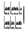
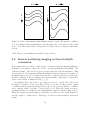
With colormapping some parts of the plot may be emphasized at the expense of other
parts. The issue of colormaps often is one of selecting the location of the “bright part”
of the colorbar, versus darker colors. Even perfectly processed data may be rendered
uninterpretable by a poor selection of colormapping. This effect may be seen in Figure 3.4.
Repeat the previous, this time clipping by percentile
$ suximage < sonar.su
legend=1
perc=99
&
The ease at which colorscales are defined, and the fact that there are no real standards
on colorscales, mean that effectively every color plot you encounter requires a colorscale
for you to be able to know what the values mean. Furthermore, some colors ranges are
brighter than others. By moving the bright color to a different part of the amplitude
range, you can totally change the image. This is a source of richness of display, but it is
also a potential source of trouble, if the proper balance of color is not chosen.
3.4
Normalization: Median balancing
A common data amplitude balancing is to balance the colorscale on the median values
in the data. The “median” is the middle value, meaning that half the values are larger
than the median value and half the data are less than the median value.
Type these commands to see that in SU:
$ sunormalize mode=med < sonar.su | suximage legend=1
$ sunormalize mode=med < sonar.su | suximage legend=1 perc=99
We will find perc=99 to be useful. Note that you may zoom in on regions of the plot
you find interesting.
31
0
200
400
0.05
4
0.10
2
0 0.15
-2
0.20
-4
0.25
Figure 3.3: Image of sonar.su data with perc=99 and legend=1.
32
Figure 3.4: Comparison of the default, hsv0, hsv2, and hsv7 colormaps. Rendering these
plots in grayscales emphasizes the location of the bright spot in the colorbar.
33
0
200
400
0.05
4
0.10
2
0 0.15
-2
0.20
-4
0.25
Figure 3.5: Image of sonar.su data with perc=99 and legend=1.
34
0
200
400
0.05
3
2 0.10
1
0 0.15
-1
-2
0.20
-3
0.25
Figure 3.6: Image of sonar.su data with median normalization and perc=99
35
Note, that if you put both the median normalized and simple perc=99 files on the
screen side-by-side, there are differences, but these may not be striking differences. The
program suximage has a feature that the user may change colormaps by pressing the
“h” key or the “r” key. Try this and you will see that the selection of the colormap can
make a considerable difference in the appearance of the image. Even with the same data,
the colormap.
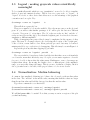
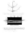
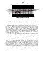
For example in Figure 3.7 we see the result of applying the commands
$ suximage < seismic.su wbox=250 hbox=600 cmap=hsv4 clip=3 title="no median" &
compared with
$ sunormalize mode=median < seismic.su
| suximage wbox=250 hbox=600 cmap=hsv4 clip=3 title="no median" &
Note that the line is broken to fit on the page. When you type this, the pipe | follows
immediately after the seismic.su. Here, the
3.5
Homework problem #1 - Due Thursday 1 Sept
2011
Repeat display gaining experiments of the previous section with “radar.su” and “seismic.su” to see what median balancing, and setting perc=... does to these data.
• Capture representative plots with axes properly labeled. You can use the Linux
screen capture feature, or find another way to capture plots into a file, (such as by
using supsimage to make PostScript plots) Feel free to use different values of perc
and different colormaps than were used in the previous examples. The OpenOffice
Word wordprocessing program is an easy program to use for this.
• Prepare a report of your results. The report should consist of:
– Your plots
– a short paragraph describing what you saw. Think of it as a figure caption.
– a listing of the actual commandlines that you ran to get the plots.
– Not more than 3 pages total!
– Make sure that your name, the due date, and the assignment number are at
the top of the first page.
• Save your report in the form of a PDF file, and email to [email protected]
36
Figure 3.7: Comparison of seismic.su median-normalized, with the same data with no
median normalization. Amplitudes are clipped to 3.0 in each case. Note that there are
features visible on the plot without median normalization that cannot be seen on the
median normalized data.
37
3.6
Concluding Remarks
There are many ways of presenting data. Two of the most important questions that
a scientist can ask when seeing a plot are ”What is the meaning of the colorscale or
grayscale of a plot?” and ”What normalization or balancing has been applied to the data
before the plot?” The answers to these questions may be as important as the answer to
the question ”What processing has been applied to these data?”
3.6.1
What do the numbers mean?
The scale divisions seen on the plots in this chapter that have been obtained by running
suximage with legend=1 show numerical values, values that are changed when we
apply display gain. Ultimately, these numbers relate to the voltage recorded from a
transducer (a geophone, hydrophone, or accelerometer). While in theory we should be
able to extract information about the size of the ground displacement in, say micrometers,
or the pressure field strength in, say megapascals there is little reason to do this. Owing
to detector and source coupling issues, and the fact that data must be gathered quickly,
we really are only interested in relative values.
38
Chapter 4
Help features in Seismic Unix
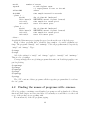
Scientific processing and data manipulation packages usually contain many commands.
Seismic Unix is no exception. As with any package there are help features to help you
navigate the collection of programs and modules. The first thing that you must do
with any software package is to locate and learn to use the help features in the package.
Usually these help mechanisms are not very “helpful” to the beginner, but are really
more like quick reference guides for people who are already familiar with the package.
There are a number of help features in SU; here we will discuss only three.
4.1
The selfdoc
All Seismic Unix programs have the feature that if the name of the program is typed
with no arguments, a self-documentation feature called a selfdoc is listed.
Try:
$
$
$
$
suplane
suximage
suxwigb
sunormalize
For example:
$ suplane
yields
SUPLANE - create common offset data file with up to 3 planes
suplane [optional parameters] >stdout
Optional Parameters:
npl=3
number of planes
nt=64
number of time samples
39
ntr=32
taper=0
number of traces
no end-of-plane taper
= 1 taper planes to zero at the end
offset
time sample interval in seconds
offset=400
dt=0.004
...plane 1 ...
dip1=0
len1= 3*ntr/4
ct1= nt/2
cx1= ntr/2
...plane 2 ...
dip2=4
len2= 3*ntr/4
ct2= nt/2
cx2= ntr/2
--More--
dip of plane #1 (ms/trace)
HORIZONTAL extent of plane (traces)
time sample for center pivot
trace for center pivot
dip of plane #2 (ms/trace)
HORIZONTAL extent of plane (traces)
time sample for center pivot
trace for center pivot
As with the Unix man pages, typing the space bar shows the rest of the help page.
Each of these programs has a relatively large number of possible argument settings. The programs “suxwigb” and “suximage” both call programs named, respectively,
“xwigb” and “ximage”. Type:
$ ximage
$ xwigb
All of the setting for “xwigb” and “ximage” apply to “suxwigb” and “suximage.”
That is a lot of settings.
Correspondingly, there are plotting programs that write out PostScript graphics output for plotting
$
$
$
$
$
$
supsimage
psimage
supswigb
pswigb
supswigp
pswigp
The “SU” versions of these programs call the respective programs that do not have
the “su” prefix.
4.2
Finding the names of programs with: suname
SU is big package containing several hundred programs as well as hundreds of library
functions, shell scripts, and associated files. Occasionally we would like to see the total
scope of the package we are working with.
For an inventory of the SU programs, typing
40
$ suname
yields
----- CWP Free Programs ----CWPROOT=/usr/local/cwp
Mains:
In CWPROOT/src/cwp/main:
* CTRLSTRIP - Strip non-graphic characters
* DOWNFORT - change Fortran programs to lower case, preserving strings
* FCAT - fast cat with 1 read per file
* ISATTY - pass on return from isatty(2)
* MAXINTS - Compute maximum and minimum sizes for integer types
* PAUSE - prompt and wait for user signal to continue
* T - time and date for non-military types
* UPFORT - change Fortran programs to upper case, preserving strings
In CWPROOT/src/par/main:
A2B - convert ascii floats to binary
B2A - convert binary floats to ascii
CSHOTPLOT - convert CSHOT data to files for CWP graphers
DZDV - determine depth derivative with respect to the velocity ",
FARITH - File ARITHmetic -- perform simple arithmetic with binary files
FTNSTRIP - convert a file of binary data plus record delimiters created
FTNUNSTRIP - convert C binary floats to Fortran style floats
GRM - Generalized Reciprocal refraction analysis for a single layer
H2B - convert 8 bit hexidecimal floats to binary
--More(3%)-Hitting the space bar shows the rest of the page. The suname output shows every
library function, shell script, and main program in the package, and may be too much
information for everyday usage.
What is more common is that we might want a bit more information than a selfdoc,
but not a complete listing. This is where the sudoc feature is useful. Typing
$ sudoc NAME
yields the sudoc entry of the program NAME.
For example we might be interested in seeing information about suplane
$ sudoc suplane
and comparing that with the selfdoc for the same program
$ suplane
41
As the number of SU programs you come in contact increases, you will find it useful
to continually be referring to the listing from suname.
The sudoc feature is an alternative to Unix man pages. The database of sudocs is
captured from the actual selfdocs in the source code automatically via a shell script, so
these do not go out of step with the actual code, the way a separately written man page
might.
4.3
Lab Activity #3 - Exploring the trace header
structure
You may have noticed that the plotting programs seem to know a lot about the data you
have been viewing. Yet, you have never been asked to give the number of samples per
trace or the number of traces. For example
$ suximage < sonar.su
perc=99
&
shows a plot without being told the dimensions of the data.
But how did the program know the number of traces and the number of samples per
trace in the data? The program knows because this, and all other SU programs read
information from a “header” that is present on each seismic trace.
4.3.1
What are the trace header fields-sukeyword?
If you type:
$ sukeyword -o
you will obtain a listing of the file segy.h, which defines the SU trace header format. The
term “segy” is derived from SEG-Y a popular data exchange standard established by the
Society of Exploration Geophysicists (SEG) in 1975 and later revised in 2005. The SU
trace header is largely the same as that defined for the SEG-Y format.
The first 240 bytes of each seismic trace in a SEG-Y dataset consist of this trace
header. The data are always uniformly sampled in time, so the “data” portion of the
trace, consisting of amplitude values only, follows immediately after the trace header.
While it may be tempting to think of a seismic section as an “array” of traces, in the
computer, these traces simply follow one after the other.
The part of the listing from sukeyword that is relevant at this point is
...skipping
typedef struct { /* segy - trace identification header */
int tracl; /* Trace sequence number within line
42
--numbers continue to increase if the
same line continues across multiple
SEG Y files.
*/
int tracr; /* Trace sequence number within SEG Y file
---each file starts with trace sequence
one
*/
int fldr; /* Original field record number */
int tracf; /* Trace number within original field record */
int ep; /* energy source point number
---Used when more than one record occurs
at the same effective surface location.
*/
int cdp; /* Ensemble number (i.e. CDP, CMP, CRP,...) */
int cdpt; /* trace number within the ensemble
---each ensemble starts with trace number one.
*/
short trid; /* trace identification code:
-1 = Other
0 = Unknown
1 = Seismic data
2 = Dead
3 = Dummy
4 = Time break
5 = Uphole
6 = Sweep
7 = Timing
8 = Water break
9 = Near-field gun signature
10 = Far-field gun signature
11 = Seismic pressure sensor
12 = Multicomponent seismic sensor
- Vertical component
13 = Multicomponent seismic sensor
- Cross-line component
43
14 = Multicomponent seismic sensor
- in-line component
15 = Rotated multicomponent seismic sensor
- Vertical component
16 = Rotated multicomponent seismic sensor
- Transverse component
17 = Rotated multicomponent seismic sensor
- Radial component
18 = Vibrator reaction mass
19 = Vibrator baseplate
20 = Vibrator estimated ground force
21 = Vibrator reference
22 = Time-velocity pairs
23 ... N = optional use
(maximum N = 32,767)
Following are CWP id flags:
109 = autocorrelation
110 = Fourier transformed - no packing
xr[0],xi[0], ..., xr[N-1],xi[N-1]
111 = Fourier transformed - unpacked Nyquist
xr[0],xi[0],...,xr[N/2],xi[N/2]
112 = Fourier transformed - packed Nyquist
even N:
xr[0],xr[N/2],xr[1],xi[1], ...,
xr[N/2 -1],xi[N/2 -1]
(note the exceptional second entry)
odd N:
xr[0],xr[(N-1)/2],xr[1],xi[1], ...,
xr[(N-1)/2 -1],xi[(N-1)/2 -1],xi[(N-1)/2]
(note the exceptional second & last entries)
113 = Complex signal in the time domain
xr[0],xi[0], ..., xr[N-1],xi[N-1]
114 = Fourier transformed - amplitude/phase
a[0],p[0], ..., a[N-1],p[N-1]
115 = Complex time signal - amplitude/phase
a[0],p[0], ..., a[N-1],p[N-1]
116 = Real part of complex trace from 0 to Nyquist
117 = Imag part of complex trace from 0 to Nyquist
118 = Amplitude of complex trace from 0 to Nyquist
119 = Phase of complex trace from 0 to Nyquist
121 = Wavenumber time domain (k-t)
44
122
123
124
125
130
143
144
145
146
147
201
202
*/
=
=
=
=
=
=
=
=
=
=
=
=
Wavenumber frequency (k-omega)
Envelope of the complex time trace
Phase of the complex time trace
Frequency of the complex time trace
Depth-Range (z-x) traces
Seismic Data, Vertical Component
Seismic Data, Horizontal Component 1
Seismic Data, Horizontal Component 2
Seismic Data, Radial Component
Seismic Data, Transverse Component
Seismic data packed to bytes (by supack1)
Seismic data packed to 2 bytes (by supack2)
short nvs; /* Number of vertically summed traces yielding
this trace. (1 is one trace,
2 is two summed traces, etc.)
*/
short nhs; /* Number of horizontally summed traces yielding
this trace. (1 is one trace
2 is two summed traces, etc.)
*/
short duse; /* Data use:
1 = Production
2 = Test
*/
int offset; /* Distance from the center of the source point
to the center of the receiver group
(negative if opposite to direction in which
the line was shot).
*/
int gelev; /* Receiver group elevation from sea level
(all elevations above the Vertical datum are
positive and below are negative).
*/
int selev; /* Surface elevation at source. */
int sdepth; /* Source depth below surface (a positive number). */
45
int gdel; /* Datum elevation at receiver group. */
int sdel; /* Datum elevation at source. */
int swdep; /* Water depth at source. */
int gwdep; /* Water depth at receiver group. */
short scalel; /* Scalar to be applied to the previous 7 entries
to give the real value.
Scalar = 1, +10, +100, +1000, +10000.
If positive, scalar is used as a multiplier,
if negative, scalar is used as a divisor.
*/
short scalco; /* Scalar to be applied to the next 4 entries
to give the real value.
Scalar = 1, +10, +100, +1000, +10000.
If positive, scalar is used as a multiplier,
if negative, scalar is used as a divisor.
*/
int
sx; /* Source coordinate - X */
int
sy; /* Source coordinate - Y */
int
gx; /* Group coordinate - X */
int
gy; /* Group coordinate - Y */
short counit; /* Coordinate units: (for previous 4 entries and
for the 7 entries before scalel)
1 = Length (meters or feet)
2 = Seconds of arc
3 = Decimal degrees
4 = Degrees, minutes, seconds (DMS)
In case 2, the X values are longitude and
the Y values are latitude, a positive value designates
the number of seconds east of Greenwich
or north of the equator
46
In case 4, to encode +-DDDMMSS
counit = +-DDD*10^4 + MM*10^2 + SS,
with scalco = 1. To encode +-DDDMMSS.ss
counit = +-DDD*10^6 + MM*10^4 + SS*10^2
with scalco = -100.
*/
short wevel; /* Weathering velocity. */
short swevel; /* Subweathering velocity. */
short sut; /* Uphole time at source in milliseconds. */
short gut; /* Uphole time at receiver group in milliseconds. */
short sstat; /* Source static correction in milliseconds. */
short gstat; /* Group static correction
in milliseconds.*/
short tstat; /* Total static applied in milliseconds.
(Zero if no static has been applied.)
*/
short laga; /* Lag time A, time in ms between end of 240byte trace identification header and time
break, positive if time break occurs after
end of header, time break is defined as
the initiation pulse which maybe recorded
on an auxiliary trace or as otherwise
specified by the recording system */
short lagb; /* lag time B, time in ms between the time break
and the initiation time of the energy source,
may be positive or negative */
short delrt; /* delay recording time, time in ms between
initiation time of energy source and time
when recording of data samples begins
(for deep water work if recording does not
start at zero time) */
short muts; /* mute time--start */
47
short mute; /* mute time--end */
unsigned short ns; /* number of samples in this trace */
unsigned short dt; /* sample interval; in micro-seconds */
short gain; /* gain type of field instruments code:
1 = fixed
2 = binary
3 = floating point
4 ---- N = optional use */
short igc; /* instrument gain constant */
short igi; /* instrument early or initial gain */
short corr; /* correlated:
1 = no
2 = yes */
short sfs; /* sweep frequency at start */
short sfe; /* sweep frequency at end */
short slen; /* sweep length in ms */
short styp; /* sweep type code:
1 = linear
2 = cos-squared
3 = other */
short stas; /* sweep trace length at start in ms */
short stae; /* sweep trace length at end in ms */
short tatyp; /* taper type: 1=linear, 2=cos^2, 3=other */
short afilf; /* alias filter frequency if used */
short afils; /* alias filter slope */
short nofilf; /* notch filter frequency if used */
48
short nofils; /* notch filter slope */
short lcf; /* low cut frequency if used */
short hcf; /* high cut frequency if used */
short lcs; /* low cut slope */
short hcs; /* high cut slope */
short year; /* year data recorded */
short day; /* day of year */
short hour; /* hour of day (24 hour clock) */
short minute; /* minute of hour */
short sec; /* second of minute */
short timbas; /* time basis code:
1 = local
2 = GMT
3 = other */
short trwf; /* trace weighting factor, defined as 1/2^N
volts for the least significant bit */
short grnors; /* geophone group number of roll switch
position one */
short grnofr; /* geophone group number of trace one within
original field record */
short grnlof; /* geophone group number of last trace within
original field record */
short gaps; /* gap size (total number of groups dropped) */
short otrav; /* overtravel taper code:
1 = down (or behind)
2 = up (or ahead) */
....
49
/* cwp local assignments */
float d1; /* sample spacing for non-seismic data */
float f1; /* first sample location for non-seismic data */
float d2; /* sample spacing between traces */
float f2; /* first trace location */
float ungpow; /* negative of power used for dynamic
range compression */
float unscale; /* reciprocal of scaling factor to normalize
range */
int ntr;
/* number of traces */
short mark; /* mark selected traces */
short shortpad; /* alignment padding */
short unass[14]; /* unassigned--NOTE: last entry causes
a break in the word alignment, if we REALLY
want to maintain 240 bytes, the following
entry should be an odd number of short/UINT2
OR do the insertion above the "mark" keyword
entry */
...
float
data[SU_NFLTS];
} segy;
Not all of these header fields get used all of the time. Some headers are more important
than others. The most relevant fields to normal SU usage are the header fields tracl,
tracr, dt, cdp, offset, sx, gx, sy, gy, and delrt.
To see the header field ranges on sonar.su, radar.su, and seismic.su type
$ surange < sonar.su
50
584 traces:
tracl
1 584 (1 - 584)
cdp
1 584 (1 - 584)
muts
75
ns
3000
dt
100
$ surange < radar.su
501 traces:
tracl
1 501 (1 - 501)
tracr
1 501 (1 - 501)
trid
1
ns
463
dt
800
hour
11
minute
3 33 (3 - 33)
sec
0 59 (41 - 7)
$ surange < seismc.su
801 traces:
tracl
1200 2000 (1200 - 2000)
tracr
67441 115081 (67441 - 115081)
fldr
594 991 (594 - 991)
tracf
1 8 (2 - 2)
ep
700 1100 (700 - 1100)
cdp
1200 2000 (1200 - 2000)
cdpt
1 8 (2 - 2)
trid
1
nhs
57 60 (60 - 60)
gelev
-10
selev
-6
scalel
1
scalco
1
sx
18212 28212 (18212 - 28212)
gx
15000 25000 (15000 - 25000)
counit
3
mute
48
ns
601
dt
4000
In each case, where four numbers appear, these are the minimum and maximum values
in the header followed by the first and last values in the data panel
You may use sukeyword to determine the meaning of any of the header field “keywords” seen here via
51
$ sukeyword
key
where ”key” is the specific keyword. For example
$ sukeyword
tracl
returns
...
int tracl;
/* Trace sequence number within line
--numbers continue to increase if the
same line continues across multiple
SEG Y files.
*/
...
The first field int tells us that this is defined as type “integer” in the header. The short
description is the SEG’s definition for this field. This can be a big deal. Ofttimes users
will want to define decimal values for the header fields.
Please note that the keyword names we use here are not an industry standard, but are
peculiar to SU. These are an invention of Einar Kjartannson, the author of the original
suite of programs call SY, that later became the basis of the SU package.
4.4
Concluding Remarks
Every data processing package has help features and internal documentation. None of
these are usually perfect, and all are usually aimed at people who already understand
the package. Look for the help features and demos of a package.
When receiving a dataset, the most important questions that a scientist can ask about
a dataset that he or she receives are: “What is the format of the data?” ”Are the data
uniformly sampled?” For seismic data: “Have the headers been set?” and “What are
ranges of the the header values?”. “Do the header values make sense?”
Note also, that data coming in from the field, frequently requires that the headers be
set in the data. Transferring header information from seismic observers logs into seismic
trace headers is called “setting geometry.” Setting geometry can be one of the biggest
headaches in preparing data for processing.
Vendors may remap the SEG-Y header fields both in terms of the meaning of the
header field and with respect to the data type. Obtaining a “header map” of data when
you obtain seismic data can prevent confusion and save you a lot of work.
When receiving data on tape, remember that “tape reading is more of an art than a
science.” It is best to ask for data in a format you can use, rather than allow someone
else to dictate that format to you.
52
Chapter 5
Lab Activity #4 Migration/Imaging as depth
conversion
Geophysical imaging, often called “migration” in the seismic context, is an example
of a general topic called “inverse-scattering imaging.” Simply stated, inverse scattering
imaging is the process of “making pictures with echos.” We have all encountered examples
of this in our daily lives. Our eyes operate by making images of the world around us
from scattered light. Medical ultrasound uses the echos of high frequency sound waves
to image structures within the human body. Ultrasound is also used in an industrial
setting for nondestructive testing (NDT). Seismic prospectors look for oil using the echos
of seismic waves. Earthquake seismologists determine the internal structure of the deep
earth with echos of waves from earthquakes. Near surface investigators use the echos of
ground penetrating radar waves to image objects in the shallow subsurface.
5.1
Imaging as the solution to an inverse problem
Acoustic and elastic waves echo off of jumps in the wavespeed and/or the density of the
medium. In the case of electromagnetic scattering, the signal is coming from a volume
of material or a layer, rather than a boundary between layers, which has a differing
conductivity from the surrounding material.
In each case, the propagating wave impinges on the boundary at some angle, and
is reflected from the boundary at an angle determined by the law of reflection for the
medium. For scalar waves, which is to say waves that do not experience mode conversion,
the angle of incidence equals the angle of reflection. For elastic waves, the angle of
reflection is a function of the angle of incidence and of the velocities and densities of the
media on either side of the reflector.
The scattered wave therefore carries information about both the orientation of the
reflector and its location. Thus, an image formed from such data is a solution to an
inverse problem wherein the wavespeed of the medium and the location and orientation
53
x
x
t
z
Figure 5.1: Cartoon showing the simple shifting of time to depth. The spatial coordinates
x do not change in the transformation, only the time scale t is stretched to the depth
scale z. Note that vertical relief looks greater in a depth section as compared with a time
section.
of the reflector are the unknown variables being solved for.
5.2
Inverse scattering imaging as time-to-depth
conversion
In geophysics there are three common types of inverse-scattering imaging techniques
that may be encountered. These are “sonar,” “ground penetrating radar (GPR),” and
“reflection seismic.” In each case a species of wave is introduced into the subsurface. This
wave is reflected off of structures within the Earth and travels back up to the surface of
the Earth where it is recorded. In the raw form, the coordinates of the data consist of the
spatial coordinates of the recording position and traveltime, which may be represented
as the ordered triple of numbers Data(x1 , x2 , t).
It is implied that some form of processing is needed to convert data collected in
the input coordinates of space and time Data(x1 , x2 , t) into an image in the output
coordinates that are purely spatial DepthImage(y1 , y2 , y3 ) or are new spatial coordinates
and a “migrated time coordinate” T imeImage(y1 , y2 , τ ). When the output is in space
and migrated time, we call the process “time migration” and the output a “time section”.
When the output is in purely spatial coordinates, we call the process “depth migration”
and the output a “depth section”. Each type of section is found useful in exploration
seismic.
54
Thus, for our “migration as depth conversion” we will consider the final step of processing as a process that converts the data from Data(y1 , y2 , τ ) to data in DepthImage(y1 , y2 , y3 )
in purely spatial coordinates.
The simplest cases of such processing occur when the output spatial coordinates on
the recording surface are such that y1 = x1 and y2 = x2 . Then the remaining problem
is to “trade time for depth”. Often the symbol z is used to represent depth, with z
increasing positively as we go deeper into the earth.
Clearly, special circumstances are needed for this simple case to exist. Effectively,
such an imaging problem is one dimensional. This type of problem may result from the
construction of synthetic well logs from migrated seismic data or making depth sections
from migrated time sections.
Sonar and GPR data usually have the attribute that the same piece of equipment is
used as both source and receiver. Furthermore, this source-receiver array is likely highly
directional, forming a beam of energy that travels straight down into the Earth. Because
the scattering occurs from roughness in the structures (“rough surface scattering”) of
the subsurface and, owing to the strength of the sources involved, we may consider the
reflection to have occurred from directly below the receiver.
To perform time-depth conversion, we need to know something about the velocities
of the subsurface.
5.3
Time-to-depth with suttoz ; depth-to-time with
suztot
The simplest approach to depth conversion is to use a simple velocity profile expressed
as a function of time v(t). How can we have velocity as a function of time? The idea is
intuitive. We expect the image to show reflectors. These reflectors are the boundaries
between media of different wavespeeds. Given auxiliary information about geology, well
logs or the result of seismic velocity analysis, we expect to be able to relate arrivals on
the seismic section to specific depth horizons, for which, in turn, we have wavespeed
information.
5.4
Time to depth conversion of a test pattern
To see what the problem of time-to-depth and depth-to-time is all about, we may try
suttoz on a test pattern made with suplane
$
$
$
$
suplane > junk.su
suttoz < junk.su t=0.0,.15,.2 v=1500,2000,3000 > junk1.su
suxwigb < junk.su title="test pattern" &
suxwigb < junk1.su title="depth section" &
The program suztot has been provided to apply depth-to-time conversion, as the
inverse of sutotz. Because we know the values of the velocity that were used, we must
55
a)
0
10
trace number
20
b)
30
10
0
trace number
20
30
0.05
100
time s
depth m
0.10
200
0.15
0.20
300
0.25
test pattern
depth section
c)
0
10
trace number
20
30
0.05
time s
0.10
0.15
0.20
time section reconstructed
Figure 5.2: a) Test pattern. b) Test pattern corrected from time to depth. c) Test
pattern corrected back from depth to time section. Note that the curvature seen depth
section indicates a non piecewise-constant v(t). Note that the reconstructed time section
has waveforms that are distorted by repeated sinc interpolation. The sinc interpolation
applied in the depth-to-time calculation has not had an anti-alias filter applied.
56
a)
1500
2000
3000
m/s
b)
0
2000
3000
velocity m/s
4000
5000
6000
500
velocity
Depth m
112.5
m
162.5
1000
1500
Well Log
c)
1500
2000
3000
m/s
velocity
131.25
193.75
m
Figure 5.3: a) Cartoon showing an idealized well log. b) Plot of a real well log. A real
well log is not well represented by piecewise constant layers. c) The third plot is a linearly
interpolated velocity profile following the example in the text. This approximation is a
better first-order approximation of a real well log.
57
try to figure out the depths Z1, Z2, and Z3, necessary to undo the operation
$ suztot < junk1.su z=Z1,Z2,Z3 v=1500,2000,3000 > junk2.su
$ suxwigb < junk2.su title="time section reconstructed" &
Please note, you don’t literally type “z=Z1,Z2,Z3” what you want is to find three numbers
representing depths to substitute in for Z1, Z2, and Z3. The first value Z1 = 0.
You will notice that on the junk1.su data, the picture does not start getting distorted
until after about depth 105. This gives a clue as to the place where the faster speeds
kick in.
You will further notice that the junk2.su data does not look very much like the
junk.su data. The first think that you should notice is that the original junk.su data
only goes to about .24 seconds, but the junk2.su data goes to more than .5 seconds.
It is a good idea to see if the header values have changed by using surange. The
original data shows
$ surange < junk.su
32 traces:
tracl
1 32 (1 - 32)
tracr
1 32 (1 - 32)
offset
400
ns
64
dt
4000
whereas the depth converted data has a greater number of samples
$ surange < junk1.su
32 traces:
tracl
1 32 (1 - 32)
tracr
1 32 (1 - 32)
trid
30
offset
400
ns
126
dt
4000
d1
3.000000
<------ ns has increased!!!
and finally, the depth-to-time converted data
$ surange < junk2.su
32 traces:
tracl
1 32 (1 - 32)
tracr
1 32 (1 - 32)
offset
400
ns
63
dt
4000
<-------- ns is now 63
shows ns=63, rather than the original ns=64 samples.
58
5.4.1
How time-depth and depth-time conversion works
The way that this works is simple. Each sample of the data is a function of time. We
have velocities to use for each time value. If the velocity is constant, then the process
of time to depth conversion is more of a relabeling process than a calculation. However,
for situations where the velocity varies as we go to later times in the data, we have to
deal with the fact that the sample spacing of the time-to-depth shifted data changes as
the velocity changes. Indeed, constant or piecewise-constant profiles rarely accurately
represent wavespeed variation in the real earth.
The depth is calculated for each sample, but because we want the output to be
uniformly sampled, we have to interpolate the missing depth values. This interpolation
may be done many ways, but in this program it is done by fitting a sinc function (sinc
interpolation) to the data points. The bandwith of this sinc function is the the band
from 0 to the Nyquist frequency of the data. When resampling to a greater number of
samples, the Nyquist frequency of the output is greater than the Nyquist frequency of the
input, so there is no possibility of aliasing. However, if we subsample data, the potential
for aliasing exists.
To repeat the test, we should be setting nt=64 to force the number of samples to be
the same on both input and output
$
$
$
$
$
$
suplane > junk.su
suttoz < junk.su t=0.0,.15,.2 v=1500,2000,3000 > junk1.su
suztot < junk1.su nt=64 z=Z1,Z2,Z3 v=1500,2000,3000 > junk2.su
suxwigb < junk.su title="test pattern" &
suxwigb < junk1.su title="depth section" &
suxwigb < junk2.su title="reconstructed time section" &
The time-to-depth may be improved by truncating the additional values
$ suwind itmax=64 < junk1.su | suxwigb title="time to depth" &
where suwind has been used to pass only the first 64 samples of each trace.
The short answer is that while the time-to-depth and depth-to-time conversions are
ostensibly simply piecewise linear operations in this simple example, the fact is that there
is the potential for errors to be introduced by the interpolation process. These errors
may make only approximately invertible process.
The main problem is deciding how the v(t) and v(z) functions are to be interpolated.
As is seen in Fig 5.3 constant step models seen in cartoon well log diagrams does not
accurately depict the complexity of actual well logs. The simplest approximation to a
real well log is a piecewise continuous curve, with piecewise linear being the simplest
curve. That is, we assume a functional form of v(t) = mt + b for velocity as a function
of time.
For the example of t = 0.0, .15, .2
v = 1500, 2000, 3000 in the region from t = 0.0
to t = .15 the velocity profile would be given by v1 (t) = (500/.15)t + 1500, and in the
region from t = .15 to t = .2, the velocity profile is given by v2 (t) = (1000/.05)t + 2000.
Calculating the values of the depths Z1, Z2, Z3, we see trivially that Z1 = 0 and that
integrating the two equations above yields Z2 = 131.25 and Z3 = 193.75, respectively.
59
5.5
Sonar and Radar, bad header values and
incomplete information
Most likely, depth conversion for sonar and radar requires simply knowing the speed of
sound in water, and the speed of light, respectively. This sounds simple, and if we had
all of the information in a neat and consistent form, it would be.
The first complication comes from the fact that SU is a seismic package. When
non-seismic data are used in a seismic package, often the time sampling interval must
be scaled to store the data. The reason for this is to save storage space in the header,
the creators of the SEG-Y data format chose the time sampling interval dt not to be a
floating point number, but rather as an unsigned short integer. On a 32 bit machine,
the size of the largest value that an unsigned short can take on is 65535. Thus, scaling
is necessary.
Usually, these scale factors are multiples of 10. Try doing depth conversion on the
sonar and radar data, using values you know for the speed of sound
$ suttoz v=SPEED_OF_SOUND_IN_WATER < sonar.su | suximage perc=99 &
and the speed of light
$ suttoz v=SPEED_OF_LIGHT < radar.su | suximage perc=99 &
respectively.
The speed of light is 2.998 × 108 m/s. The speed of sound in water is 1500m/s. Likely,
the correct values to use in each case will be off by some multiple of 10, owing to the
fact that the natural frequencies available for radar and sonar are not in the same band
as those used for seismic data.
If we type
$ sukeyword dt
...
unsigned short dt;
..
/* sample interval; in micro-seconds */
we see that the time sampling interval, dt, is expressed in microseconds. Seismic frequencies range from a few Hz, to maybe 200 hz, but likely are not up into the kilohertz
range, unless some special survey is being conducted. Sonar frequencies likely range ten’s
of kilohertz to hundreds of kilohertz. Radar operates in the megahertz range. So, it is
common for the user to fake the units on the time sampling interval so as to fit the
requirements of a seismic code.
5.6
The sonar data
The “sonar.su” file is one of the profiles collected by Dr. Henrique Tono of Duke University in a special laboratory setting.
60
According to a personal communication by Dr. Tono, the “geologic setting” of the
sonar data is thus
“The deposits and images were produced at the Saint Anthony Falls Lab of
the University of Minnesota. Here, experimental stratigraphy is produced
under precisely controlled conditions of subsidence, base level, and sediment
supply. By superimposing optical images of the sectioned deposits on seismic
images, we can directly observe the ability of seismic profiling to distinguish
different geological features.
The experimental basin is 5 m by 5 m (25 m2) and 0.61 m deep. Sediment
and water were mixed in a funnel and fed into the basin at one corner. This
produced an approximately radially-symmetrical fluvial system, which averaged 2.50 m from source to shoreline. The edges of the basin were artificially
roughened in order to direct the channels away from the walls. The ”ocean
level” was maintained through a variable-discharge siphon located in the opposite corner of the basin. Though we imposed a gradual base-level rise, in
order to simulate subsidence, the shoreline maintained a constant position
through the experiment.”
Dr. Tono goes on to describe the experimental layout:
”The outgoing pulse is generated with a Prototype JRS DPR300 (Pulser/Receiver),
which drives a 900-volt square pulse into the transducer. It is set to a
pulse/receive frequency of 100 Hz, with an input gain of 30 dB in echo mode.
The high pass filter is set at 20 KHz, and the low pass filter at 10 MHz. A
Gage-Applied Compuscope 1602 digitizer computer card (16 Bit, 2 Channel
card with acquisition memory of 1 Million samples) is used to perform the
A/D conversion, and the data is displayed on a computer screen by means
of GageScope 3.50. It is digitally recorded on the computer hard disk. A
sample rate of 2.5 MS/s is chosen (Nyquist frequency=1.25 MHz). It is then
re-formatted to SEG-Y and processed with Seismic Unix.
The data were acquired with a 5mm shotpoint and station interval (zero
offset), and 1cm separation between lines.”
In the directory /cwpscratch/Data1 you will find a number of JPEG format files
depicting the experimental setting described by Dr. Tono.
The file ”dsc01324.su” is an SU format file version of the image DSC01324.JPG,
cropped to remove parts of the image that are not the cross section. This is not exactly
the cross section of the data sonar.su, but it gives the idea. Rarely, are we able to slice
into the actual model in this fashion.
61
5.7
Homework Problem - #2 - Time-to-depth
conversion of the sonar.su and the radar.su
data. Due Thursday 8 Sept 2011
Find the necessary velocities to permit the correct time-to-depth conversion of the sonar.su
and radar.su data. You will need to figure out the appropriate units, because it is not
possible for these non-seismic datasets to have an accurate representation of the time
sampling interval represented in the trace header field dt. Make sure that you give a
justification explaining why your choice of the appropriate power of 10 scaling factor is
likely the correct one. Remember that the depth scale on you output data should make
sense.
5.8
Concluding Remarks
When receiving software, either that is given to us, or that which we purchase, it is
important to try to figure out what assumptions are built into the software. One way to
do that is to try the software out on test patterns.
When receiving data, it is important to know everything that you can possibly know
about the data, such as the spacing of the traces, the time sampling interval, any processing that has been applied.
When explaining seismic imaging to non-geophysicists, it is tempting to say that seismic imaging is “sort of like sonar”. However, sonar is a rough-surface-scattering imaging,
whereas seismic is a “specular” or mirror-reflection-scattering imaging. In rough-surface
scattering, the image may, indeed, be formed by ”straight down and straight back” reflections. In seismic, this is rarely the case. We must take offset between the source and
receiver into account. In seismic, there are also rough-surface contributions. These are
the diffractions we look for on stacked data.
In the early days of seismic (well into the 1930s) there were practitioners of the seismic
method, who thought that seismic was like sonar and expected that seismic datasets
should be “data images.”
62
Chapter 6
Zero-offset (aka poststack) migration
The first reflection seismic experiment as applied to the petroleum exploration was conducted by physicist John Clarence Karcher in Oklahoma in 1921. Oklahoma was the
center of the US oil industry at that time. It is clear from reading documents from that
era that the expectations of reflection seismic methods were that the results should be
similar to sonar. That is, the expectation was that the signal would travel straight down
into the subsurface, reflect off of a few structures, and then travel straight back up to be
recorded. There was no expectation of off-vertical reflections.
We of course know that this is not the case. By the 1930s many geophysicists were
well aware of the geometrical issues at the heart of proper seismic interpretation. With
the formation of the Society of Exploration Geophysicists in 1930, followed by the first
issue of the Society’s journal Geophysics the proper usage of seismic data for geologic
interpretation became known to the geophysical community.
In Figure 6.1 we see the classical “bowtie” feature seen over a syncline. To the
early interpreter of seismic data, this diagram would not have constituted an image of
the subsurface, but rather a source of geometrical data (such as dip) pertaining the
subsurface reflector.
Another notion that became apparent is that parts of the data on the seismic traces
is displaced from its “correct” position by the properties of wave propagation. Assuming
that all reflections are normal incidence for this zero-offset geometry, it is clear that
parts of the bowtie originate from higher positions on the sides of the syncline. Thus,
the notion of “migrating” those arrivals to their correct location became an important
idea for interpretation. Because the seismic data were analog rather than digital, such
corrections would naturally be applied graphically.
While graphical migration techniques had been applied since the 1930s, the first
notable technical paper describing this technique was published by J. G. (Mendel) Hagedoorn in 1954. This paper is important because Hagedoorn’s description of the migration
process inspired early digital computer implementations of migration.
63
a)
20
Time in Seconds
0
Trace
40
60
80
1
Synthetic Seismogram
Depth (m)
b)
0
0
1000
Range (m)
2000
v = 2000 m/s
ρ = const.
v = 3000 m/s
ρ = const.
3000
1000
2000
Simple Single-Reflector Model
Figure 6.1: a) Synthetic Zero offset data. b) Simple earth model.
64
4000
6.1
Migration as reverse time propagation.
One way of looking at migration is as a reverse time propagation. The idea may be
visualized by running the output from a forward modeling demo in reverse time. Do the
following, noting that you need to replace “yourusername” with your actual username
on the system, so that the items are copied to your personal scratch area
$ cp /cwpscratch/Data1/syncline.unif2 /scratch/yourusername/Temp1
$ cp /cwpscratch/Data1/XSyncline /scratch/yourusername/Temp1
Now
$ cd /scratch/yourusername/Temp1
If you type:
$ more syncline.unif2
0
0
4000
0
1
-99999
0
1000.
500.
1100.
1000.
1300.
2000.
1000.
2700.
1100.
3200.
1000.
4000.
1050.
1.
-99999
you will see the input data for a wavespeed profile building program called unif2. The
contents of this file define two boundaries in a velocity model. The data for the two
boundaries is separated by the values
1.
-99999
The values in the column on the left are horizontal positions and the values on the right
are depths. This model defines the same simple syncline model seen in Fig 6.1. We now
look at the contents of the shell script XSyncline
$ more XSyncline
#! /bin/sh
# Shell script to build velocity profiles with unif2
# input parameters
modelfile=syncline.unif2
velfile=syncline.bin
65
n1=200
n2=400
d1=10
d2=10
# use unif2 to build the velocity profile
unif2 <$modelfile method=$i ninf=2 nx=$n2 nz=$n1 v00=1000,2000 \
ninf=1 method=spline > $velfile
# view the velocity profile on the screen
ximage < $velfile wbox=400 hbox=200 n1=$n1 n2=$n2 d1=$d1 d2=$d2 \
wbox=800 hbox=400 legend=1 title="Syncline model" label1="depth m" \
label2="distance m " units="m/s" &
# provide input for sufdmod2
xs=1000 zs=10 hsz=10 vsx=1000 verbose=2
vsfile="vseis.su" ssfile="sseis.su" hsfile="hseis.su"
tmax=3.0 mt=10
label1="Depth m"
label2="Distance m"
# perform finite difference acoustic modeling to generate data
# for a single shot in the
sufdmod2 < $velfile nz=$n1 dz=$d1 nx=$n2 dx=$d2 verbose=1 \
xs=$xs zs=$zs hsz=$hsz vsx=$vsx hsfile=$hsfile \
vsfile=$vsfile ssfile=$ssfile verbose=$verbose \
tmax=$tmax abs=1,1,1,1 mt=$mt |
suxmovie clip=1.0 \
title="Acoustic Finite-Differencing" \
windowtitle="Movie" \
label1=$label1 label2=$label2 \
n1=$n1 d1=$d1 f1=$f1 n2=$n2 d2=$d2 f2=$f2 \
loop=1 sleep=20000 -geometry 800x400 &
exit 0
You may run the demo by typing:
$ XSyncline
The result shows the wavespeed profile for the model. This is similar to the “simple”
model that will be discussed later in the these notes. A movie showing snapshots of
the wavefield will begin. Watch the wavefront of the energy from the shot expand. You
may stop and restart the movie by pressing the far right mouse button. Of interest are
the frames at which the first reflections begin. As the movie progresses, you will see
66
the reflected field progress as the reflection point propagates along the reflector surface.
Indeed, from viewing this movie, we can see why an integral over the reflector surface,
called the “Kirchhoff modeling formula” is a way of modeling the reflected field.
Note that you only see wavefronts, there is nothing like a “ray” to be seen. A ray is
the trajectory taken by a point on a wavefront. Second, notice that the “bowtie” forms
as the caustic in the propagating wavefield.
The movie will run in a loop. You may stop the movie by pushing the right mouse
button. You may reverse the movie by pressing the middle mouse button. Effectively,
running the field backward in time is “reverse-time migration.” In seismic data, we do
not have a record of the down-traveling field. All we have is the record of that part
of the reflected field that hits the surface of the earth where there are geophones. The
migration process finds the place where the downtravelling field and the reflected field
overlay—the reflector surface. One way of looking at migration is that we would like to
cross-correlate the down-traveling field with the time-reversed reflected field. The place
where these fields correlate is at the reflector surface.
You may also see what the seismic data looks like recorded at the surface of the earth
model by viewing the file hseis.su via
$ suximage < hseis.su perc=99
to see the direct arrival and the bowtie-shaped reflected arrival.
Finally you may change the depths in the model by editing the file syncline.unif2,
or change the location of the source to see what varying these quantities changes in the
data. You may slow down the movie by increasing the value of the sleep= parameter.
6.2
Lab Activity #5 - Hagedoorn’s graphical
migration
The purpose of this lab example is to migrate the simple data in Figure 6.1a) by Hagadoorn’s graphical method. These synthetic data represent the zero-offset reflection
seismograms recorded over the undulating reflector model in Figure 6.1b). The wavespeed in the upper medium is assumed to be 2000 m/s, and the data are drawn in such
a way that 1.0 s two way time is equivalent to 1000 m of distance. Thus, the time scale
translates into a depth scale that is compatible with the horizontal scale.
If we draw a circle centered at time t = 0 of a given seismic trace and passing through
a given seismic arrival, we have sketched all possible reflection points from which the
seismic arrival could have originated. These circles are the same as the incident field seen
in the seismic movie. If we recall, seismic migration finds the place where the incident
field interacts with the reflected field—the reflector surface.
When similar circles are drawn for every arrival on every trace, the result is a collection
of circles whose envelope delineates the reflector. See Fig 6.3 for an idea of what this
should look like.
67
t=0.0
Figure 6.2: The Hagedoorn method applied to the arrivals on a single seismic trace.
20
60
80
Time in Seconds
0
Trace
40
2
Synthetic Seismogram
Figure 6.3: Hagedoorn’s method applied to the simple data of Fig 6.1. Here circles, each
centered at time t = 0 on a specific trace, pass through the maximum amplitudes on
each arrival on each trace. The circle represents the locus of possible reflection points in
(x, z) where the signal in time could have originated.
68
20
60
80
Time in Seconds
0
Trace
40
2
Synthetic Seismogram
Figure 6.4: The dashed line is the interpreted reflector taken to be the envelope of the
circles.
Mathematically this method of migration may be thought of as the reconstruction of
the reflector by defining the tangent vectors of the reflector. What then, are the circles we
have drawn? The answer can by found by looking at Figure 6.5. For our 2D constantwavespeed example, all solutions of the wave equation, which is to say all wavefronts,
can be found by passing a horizontal plane through the cone in Figure 6.5. Both physical
(causal) solutions (the positive t cone) and the nonphysical (anti-causal) solutions (the
negative t cone) are depicted. We use the causal cone for modeling, and the anti-causal
or reverse-time cone for migration.
To see what a given circle means in Hagadoorn’s method, we may look at the reverse
time cone in Figure 6.6. We may think of the curve on the t = 0-plane as the locus of
all possible positions from which the reflection originated, or we may think of this as the
wavefront of the backward-propagated wave.
If we were to apply the Hagedoorn method on the computer, we might consider
creating for each seismic trace a panel of seismic traces replicating our original seismic
arrivals, but on a semicircular pattern. “Spraying” out our seismic data for each trace
along the respective Hagedoorn circle would yield one new panel of traces for each seismic
trace. Our 80 traces would then become 80 panels of sprayed traces. We would then
sum the corresponding traces on each panel. Constructive interference would tend to
enhance the region near the reflector, and destructive interference would tend to eliminate
everything else, revealing only the reflector. Does this method work? Yes, but it is subject
to interference errors, if the data are not densely sampled in space.
Because a point at (ξ, τ ) represents an impulse in the (x, t) space, corresponding
69
z
x
t
Figure 6.5: The light cone representation of the constant-velocity solution of the 2D wave
equation. Every wavefront for both positive and negative time t is found by passing a
plane parallel to the (x, z)-plane through the cone at the desired time t. We may want
to run time backwards for migration.
z
x
t
(ξ,τ)
Figure 6.6: The light cone representation for negative times is now embedded in the
(x, z, t)-cube. A seismic arrival to be migrated at the coordinates (ξ, τ ) is placed at the
apex of the cone. The circle that we draw on the seismogram for that point is the set of
points obtained by the intersection of the cone with the t = 0-plane.
70
Time (sec)
0
1
2
Distance (km)
3
4
5
6
2
Diffraction
Figure 6.7: Hagedoorn’s method of graphical migration applied to the diffraction from
a point scatterer. Only a few of the Hagedoorn circles are drawn, here, but the reader
should be aware that any Hagedoorn circle through a diffraction event will intersect the
apex of the diffraction hyperbola.
circle drawn in Hagadoorn’s method may be thought of as the impulse response of the
migration operation.
6.3
Migration as a Diffraction stack
Another approach to migration is immediately apparent. If we apply Hagedoorn’s method
to the diffraction from a point scatterer, then we observe that the scatterer is reconstructed. However, tangent vectors are not defined with regard to a point scatter. Instead, it must be the vector from the source/receiver position to the scatterer that is being
reconstructed. In other words, the reflected ray vector is the distinguished vector associated with the imaging point. For a reflector surface, this is the perpendicularly-reflected
ray vector. See Figure 6.7.
Furthermore, we might ask: why is it necessary to draw Hagedoorn’s circles at all?
Suppose that we were to sum over all possible diffraction hyperbolae. Then the largest
arrivals would exist only where a hyperbola we sum on hits a hyperbola in the data. The
sum would then be placed at a point at the apex of the hyperbola passing through our
data. This type of migration is referred to as a diffraction stack. We sum or “stack”
data, but we do this over a diffraction curve. Furthermore the output need not be a
71
x
(x,z)
z
t
Figure 6.8: The light cone for a point scatterer at (x, z). By classical geometry, a vertical
slice through the cone in (x, t) (the z = 0 plane where we record our data) is a hyperbola.
depth section, but could be a time section.
A useful diagram for understanding the diffraction stack is the light cone diagram in
Figure 6.8. A light cone is the representation of the surface where solutions of the wave
equation live. The scatterer is located at the point (x, z). Time increases downward. A
horizontal slice through the cone reveals the circular wavefronts that are the circles drawn
in Hagedoorn’s method. A vertical slice through the cone in (x, t) reveals the hyperbola
that is the characteristic shape of a diffraction in a constant wavespeed medium.
6.4
Migration as a mathematical mapping
Another diagram that reveals migration as a type of data transformation or mapping may
be seen in Figure 6.9. Here, we see that the impulse response of the migration operator
is a circular curve in constant wavespeed media.
The diffraction in (x, t) may be thought of as the “impulse response” of the modeling
operation that made the data from a point at (x, z). Migration by diffraction stack,
therefore, consists of selecting a point (x, z), modeling the diffraction curve in (x, t), and
then summing through the data over this curve. Note that this must be done for every
output point to make the image.
Figure 6.9 represents more than migration. Going from a) to b) is Hagedoorn’s
migration method. Going from c) to d is the diffraction stack migration method. If
however, we reverse directions, mapping from from b) to a) or from d) to c then we are
modeling or doing data-based de-migration, which is the inverse of migration. The idea
then is that modeling is the forward process and migration is the inverse operation.
72
a)
t
c)
x
b)
(ξ,τ)
z
x
d)
z
t
x
x
(x,z)
Figure 6.9: Cartoon showing the relationship between types of migration. a) shows a
point in (ξ, τ ), b) the impulse response of the migration operation in (x, z), c) shows a
diffraction, d) the diffraction stack as the output point (x, z).
6.5
Concluding Remarks
The notion of the value and motivation of using seismic data has changed through the
history of seismic methods. Originally, seismic data were used to find estimates of depth
of perhaps a single important horizon. As the technique developed, the depth to and dip
of a specific target reflector was found. Most notably was Frank Rieber’s “dip finder.”
The “dip finder” was a recording system that was effectively an analog computer that
delivered an estimate of depth and dip for stronger reflectors. These data were then
used for drawing geologic cross-sections. In fact, Frank Rieber’s dip finder was doing
something similar to a variety of migration called “map migration.”
As the petroleum and natural gas industry evolved, so did the importance of the
seismic method. The technique started out as an aid in interpretation, becoming later
an “imaging technology.” Today, seismic migration is viewed by many as the “solution
to an inverse problem” wherein recorded seismic data are used as input to solve for
the reflectivity of the reflectors, as well as other important material parameters that
characterize lithology.
73