Download Semi-Automatic Classification Plugin Documentation

Semi-Automatic Classification Plugin
Documentation
Release 4.8.0.1
Luca Congedo
October 29, 2015
Contents
I
Plugin Installation
3
1
Installation in Windows 32 bit
1.1 QGIS download and installation . . . . . . . . . .
1.2 Semi-Automatic Classification Plugin installation .
1.3 Configuration of the plugin . . . . . . . . . . . .
1.4 Known issues . . . . . . . . . . . . . . . . . . . .
.
.
.
.
7
7
7
8
9
2
Installation in Windows 64 bit
2.1 QGIS download and installation . . . . . . . . . . . . . . . . . . . . . . . . . . . . . . . . . . .
2.2 Semi-Automatic Classification Plugin installation . . . . . . . . . . . . . . . . . . . . . . . . . .
2.3 Configuration of the plugin . . . . . . . . . . . . . . . . . . . . . . . . . . . . . . . . . . . . .
11
11
11
12
3
Installation in Ubuntu Linux
3.1 QGIS download and installation . . . . . . . . . . . . . . . . . . . . . . . . . . . . . . . . . . .
3.2 Semi-Automatic Classification Plugin installation . . . . . . . . . . . . . . . . . . . . . . . . . .
3.3 Configuration of the plugin . . . . . . . . . . . . . . . . . . . . . . . . . . . . . . . . . . . . .
15
15
15
16
4
Installation in Debian Linux
4.1 QGIS download and installation . . . . . . . . . . . . . . . . . . . . . . . . . . . . . . . . . . .
4.2 Semi-Automatic Classification Plugin installation . . . . . . . . . . . . . . . . . . . . . . . . . .
4.3 Configuration of the plugin . . . . . . . . . . . . . . . . . . . . . . . . . . . . . . . . . . . . .
19
19
19
20
5
Installation in Mac OS
5.1 QGIS download and installation . . . . . . . . . . . . . . . . . . . . . . . . . . . . . . . . . . .
5.2 Semi-Automatic Classification Plugin installation . . . . . . . . . . . . . . . . . . . . . . . . . .
5.3 Configuration of the plugin . . . . . . . . . . . . . . . . . . . . . . . . . . . . . . . . . . . . .
23
23
23
24
II
6
7
.
.
.
.
.
.
.
.
.
.
.
.
.
.
.
.
.
.
.
.
.
.
.
.
.
.
.
.
.
.
.
.
.
.
.
.
.
.
.
.
.
.
.
.
.
.
.
.
.
.
.
.
.
.
.
.
.
.
.
.
.
.
.
.
.
.
.
.
.
.
.
.
.
.
.
.
.
.
.
.
.
.
.
.
.
.
.
.
.
.
.
.
.
.
.
.
Brief Introduction to Remote Sensing
Basic Definitions
6.1 GIS definition . . . . . .
6.2 Remote Sensing definition
6.3 Sensors . . . . . . . . . .
6.4 Radiance and Reflectance
6.5 Spectral Signature . . . .
6.6 Landsat Satellite . . . . .
6.7 Sentinel-2 Satellite . . . .
6.8 Color Composite . . . . .
6.9 Pan-sharpening . . . . . .
27
.
.
.
.
.
.
.
.
.
31
31
31
33
33
33
34
34
35
35
Supervised Classification Definitions
7.1 Land Cover . . . . . . . . . . . . . . . . . . . . . . . . . . . . . . . . . . . . . . . . . . . . . .
39
39
.
.
.
.
.
.
.
.
.
.
.
.
.
.
.
.
.
.
.
.
.
.
.
.
.
.
.
.
.
.
.
.
.
.
.
.
.
.
.
.
.
.
.
.
.
.
.
.
.
.
.
.
.
.
.
.
.
.
.
.
.
.
.
.
.
.
.
.
.
.
.
.
.
.
.
.
.
.
.
.
.
.
.
.
.
.
.
.
.
.
.
.
.
.
.
.
.
.
.
.
.
.
.
.
.
.
.
.
.
.
.
.
.
.
.
.
.
.
.
.
.
.
.
.
.
.
.
.
.
.
.
.
.
.
.
.
.
.
.
.
.
.
.
.
.
.
.
.
.
.
.
.
.
.
.
.
.
.
.
.
.
.
.
.
.
.
.
.
.
.
.
.
.
.
.
.
.
.
.
.
.
.
.
.
.
.
.
.
.
.
.
.
.
.
.
.
.
.
.
.
.
.
.
.
.
.
.
.
.
.
.
.
.
.
.
.
.
.
.
.
.
.
.
.
.
.
.
.
.
.
.
.
.
.
.
.
.
.
.
.
.
.
.
.
.
.
.
.
.
.
.
.
.
.
.
.
.
.
.
.
.
.
.
.
.
.
.
.
.
.
.
.
.
.
.
.
.
.
.
.
.
.
.
.
.
.
.
.
.
.
.
.
.
.
.
.
.
.
.
.
.
.
.
.
.
.
.
.
.
.
.
.
.
.
.
.
.
.
.
.
.
.
.
.
.
.
.
.
.
.
.
.
.
i
7.2
7.3
7.4
7.5
7.6
7.7
7.8
8
9
III
Supervised Classification .
Training Areas . . . . . .
Classes and Macroclasses
Classification Algorithms
Spectral Distance . . . . .
Classification Result . . .
Accuracy Assessment . .
.
.
.
.
.
.
.
.
.
.
.
.
.
.
.
.
.
.
.
.
.
.
.
.
.
.
.
.
.
.
.
.
.
.
.
.
.
.
.
.
.
.
.
.
.
.
.
.
.
.
.
.
.
.
.
.
.
.
.
.
.
.
.
.
.
.
.
.
.
.
.
.
.
.
.
.
.
.
.
.
.
.
.
.
.
.
.
.
.
.
.
.
.
.
.
.
.
.
.
.
.
.
.
.
.
.
.
.
.
.
.
.
.
.
.
.
.
.
.
.
.
.
.
.
.
.
.
.
.
.
.
.
.
.
.
.
.
.
.
.
.
.
.
.
.
.
.
.
.
.
.
.
.
.
.
.
.
.
.
.
.
.
.
.
.
.
.
.
.
.
.
.
.
.
.
.
.
.
.
.
.
.
.
.
.
.
.
.
.
.
.
.
.
.
.
.
.
.
.
.
.
.
.
.
.
.
.
.
.
.
.
.
.
.
.
.
.
.
.
.
.
.
.
.
.
.
.
.
.
.
.
.
.
.
.
.
.
.
.
.
.
.
.
.
.
.
.
.
.
.
.
.
.
.
.
.
.
.
.
.
.
.
.
.
.
.
39
39
39
40
42
44
44
Landsat image conversion to reflectance and DOS1 atmospheric correction
8.1 Radiance at the Sensor’s Aperture . . . . . . . . . . . . . . . . . . . . .
8.2 Top Of Atmosphere (TOA) Reflectance . . . . . . . . . . . . . . . . . .
8.3 Surface Reflectance . . . . . . . . . . . . . . . . . . . . . . . . . . . .
8.4 DOS1 Correction . . . . . . . . . . . . . . . . . . . . . . . . . . . . . .
.
.
.
.
.
.
.
.
.
.
.
.
.
.
.
.
.
.
.
.
.
.
.
.
.
.
.
.
.
.
.
.
.
.
.
.
.
.
.
.
.
.
.
.
.
.
.
.
.
.
.
.
47
47
47
48
48
Conversion to At-Satellite Brightness Temperature
51
Basic Tutorials
53
10 Tutorial 1: Your First Land Cover Classification
10.1 Data . . . . . . . . . . . . . . . . . . . . . . . . . .
10.2 Load Data . . . . . . . . . . . . . . . . . . . . . .
10.3 Set the Input Image in SCP . . . . . . . . . . . . .
10.4 Create the Training Shapefile and Signature List File
10.5 Create the ROIs . . . . . . . . . . . . . . . . . . .
10.6 Create a Classification Preview . . . . . . . . . . .
10.7 Create the Classification Output . . . . . . . . . . .
.
.
.
.
.
.
.
.
.
.
.
.
.
.
.
.
.
.
.
.
.
.
.
.
.
.
.
.
.
.
.
.
.
.
.
.
.
.
.
.
.
.
.
.
.
.
.
.
.
.
.
.
.
.
.
.
.
.
.
.
.
.
.
.
.
.
.
.
.
.
.
.
.
.
.
.
.
.
.
.
.
.
.
.
.
.
.
.
.
.
.
.
.
.
.
.
.
.
.
.
.
.
.
.
.
.
.
.
.
.
.
.
.
.
.
.
.
.
.
.
.
.
.
.
.
.
.
.
.
.
.
.
.
.
.
.
.
.
.
.
.
.
.
.
.
.
.
.
.
.
.
.
.
.
.
.
.
.
.
.
.
.
.
.
.
.
.
.
57
57
57
58
58
58
61
61
11 Tutorial 2: Land Cover Classification of Landsat Images
11.1 Data Download . . . . . . . . . . . . . . . . . . . . .
11.2 Automatic Conversion to Surface Reflectance . . . . .
11.3 Clip Data . . . . . . . . . . . . . . . . . . . . . . . .
11.4 Create the Band Set . . . . . . . . . . . . . . . . . .
11.5 Open the Training Shapefile and Signature List File .
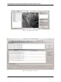
11.6 Create the ROIs . . . . . . . . . . . . . . . . . . . .
11.7 Create a Classification Preview . . . . . . . . . . . .
11.8 Assess Spectral Signatures . . . . . . . . . . . . . . .
11.9 Create the Classification Output . . . . . . . . . . . .
.
.
.
.
.
.
.
.
.
.
.
.
.
.
.
.
.
.
.
.
.
.
.
.
.
.
.
.
.
.
.
.
.
.
.
.
.
.
.
.
.
.
.
.
.
.
.
.
.
.
.
.
.
.
.
.
.
.
.
.
.
.
.
.
.
.
.
.
.
.
.
.
.
.
.
.
.
.
.
.
.
.
.
.
.
.
.
.
.
.
.
.
.
.
.
.
.
.
.
.
.
.
.
.
.
.
.
.
.
.
.
.
.
.
.
.
.
.
.
.
.
.
.
.
.
.
.
.
.
.
.
.
.
.
.
.
.
.
.
.
.
.
.
.
.
.
.
.
.
.
.
.
.
.
.
.
.
.
.
.
.
.
.
.
.
.
.
.
.
.
.
.
.
.
.
.
.
.
.
.
.
.
.
.
.
.
.
.
.
.
.
.
.
.
.
.
.
.
.
.
.
.
.
.
.
.
.
65
65
66
69
71
71
73
78
78
79
12 Other Tutorials
81
IV
83
The Interface of SCP
13 SCP menu
85
14 Toolbar
87
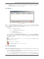
15 ROI Creation dock
15.1 Training shapefile . . .
15.2 ROI list . . . . . . . . .
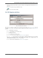
15.3 ROI parameters . . . . .
15.4 ROI creation . . . . . .
15.5 ROI Signature definition
.
.
.
.
.
.
.
.
.
.
.
.
.
.
.
.
.
.
.
.
.
.
.
.
.
.
.
.
.
.
.
.
.
.
.
.
.
.
.
.
.
.
.
.
.
.
.
.
.
.
.
.
.
.
.
.
.
.
.
.
.
.
.
.
.
.
.
.
.
.
.
.
.
.
.
.
.
.
.
.
.
.
.
.
.
.
.
.
.
.
.
.
.
.
.
.
.
.
.
.
.
.
.
.
.
.
.
.
.
.
.
.
.
.
.
.
.
.
.
.
.
.
.
.
.
.
.
.
.
.
.
.
.
.
.
.
.
.
.
.
.
.
.
.
.
.
.
.
.
.
.
.
.
.
.
.
.
.
.
.
.
.
.
.
.
.
.
.
.
.
.
.
.
.
.
.
.
.
.
.
.
.
.
.
.
.
.
.
.
.
.
.
.
.
.
89
89
91
91
92
93
16 Classification dock
16.1 Signature list file . . . .
16.2 Signature list . . . . . .
16.3 Classification algorithm
16.4 Classification preview .
.
.
.
.
.
.
.
.
.
.
.
.
.
.
.
.
.
.
.
.
.
.
.
.
.
.
.
.
.
.
.
.
.
.
.
.
.
.
.
.
.
.
.
.
.
.
.
.
.
.
.
.
.
.
.
.
.
.
.
.
.
.
.
.
.
.
.
.
.
.
.
.
.
.
.
.
.
.
.
.
.
.
.
.
.
.
.
.
.
.
.
.
.
.
.
.
.
.
.
.
.
.
.
.
.
.
.
.
.
.
.
.
.
.
.
.
.
.
.
.
.
.
.
.
.
.
.
.
.
.
.
.
.
.
.
.
.
.
.
.
.
.
.
.
.
.
.
.
.
.
.
.
.
.
.
.
95
95
95
97
98
ii
16.5 Classification style . . . . . . . . . . . . . . . . . . . . . . . . . . . . . . . . . . . . . . . . . .
16.6 Classification output . . . . . . . . . . . . . . . . . . . . . . . . . . . . . . . . . . . . . . . . .
17 Main Interface Window
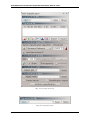
17.1 Tools . . . . . . .
17.2 Pre processing . .
17.3 Post processing . .
17.4 Band calc . . . . .
17.5 Band set . . . . .
17.6 Settings . . . . . .
.
.
.
.
.
.
.
.
.
.
.
.
.
.
.
.
.
.
.
.
.
.
.
.
.
.
.
.
.
.
.
.
.
.
.
.
.
.
.
.
.
.
.
.
.
.
.
.
.
.
.
.
.
.
.
.
.
.
.
.
.
.
.
.
.
.
.
.
.
.
.
.
.
.
.
.
.
.
.
.
.
.
.
.
.
.
.
.
.
.
.
.
.
.
.
.
.
.
.
.
.
.
.
.
.
.
.
.
.
.
.
.
.
.
.
.
.
.
.
.
.
.
.
.
.
.
.
.
.
.
.
.
.
.
.
.
.
.
.
.
.
.
.
.
.
.
.
.
.
.
.
.
.
.
.
.
.
.
.
.
.
.
.
.
.
.
.
.
.
.
.
.
.
.
.
.
.
.
.
.
.
.
.
.
.
.
.
.
.
.
.
.
.
.
.
.
.
.
.
.
.
.
.
.
.
.
.
.
.
.
.
.
.
.
.
.
.
.
.
.
.
.
.
.
.
.
.
.
.
.
.
.
.
.
.
.
.
.
.
.
.
.
.
.
.
.
.
.
.
.
.
.
99
99
101
102
114
117
125
127
129
18 Spectral Signature Plot
135
18.1 Plot Signature list . . . . . . . . . . . . . . . . . . . . . . . . . . . . . . . . . . . . . . . . . . 136
19 Scatter Plot
141
19.1 ROI List . . . . . . . . . . . . . . . . . . . . . . . . . . . . . . . . . . . . . . . . . . . . . . . 142
V
Thematic Tutorials
20 Tutorial: Land Cover Classification and Mosaic of Several Landsat images
20.1 Plugin installation . . . . . . . . . . . . . . . . . . . . . . . . . . . . .
20.2 Download and Pre processing of Landsat images . . . . . . . . . . . . .
20.3 Classification of Landsat Images . . . . . . . . . . . . . . . . . . . . . .
20.4 Enhancement of Classification Using NDVI . . . . . . . . . . . . . . . .
20.5 Cloud Masking . . . . . . . . . . . . . . . . . . . . . . . . . . . . . . .
20.6 Mosaic of Classifications . . . . . . . . . . . . . . . . . . . . . . . . . .
20.7 Accuracy Assessment . . . . . . . . . . . . . . . . . . . . . . . . . . .
20.8 Clip of the Classification . . . . . . . . . . . . . . . . . . . . . . . . . .
20.9 Classification Report . . . . . . . . . . . . . . . . . . . . . . . . . . . .
145
.
.
.
.
.
.
.
.
.
.
.
.
.
.
.
.
.
.
.
.
.
.
.
.
.
.
.
.
.
.
.
.
.
.
.
.
.
.
.
.
.
.
.
.
.
.
.
.
.
.
.
.
.
.
.
.
.
.
.
.
.
.
.
.
.
.
.
.
.
.
.
.
.
.
.
.
.
.
.
.
.
.
.
.
.
.
.
.
.
.
.
.
.
.
.
.
.
.
.
.
.
.
.
.
.
.
.
.
.
.
.
.
.
.
.
.
.
149
149
150
155
167
170
173
173
174
175
21 Tutorial: Using the tool Band calc
179
21.1 Application of a mask to multiple bands . . . . . . . . . . . . . . . . . . . . . . . . . . . . . . . 179
21.2 NDVI Calculation . . . . . . . . . . . . . . . . . . . . . . . . . . . . . . . . . . . . . . . . . . 181
21.3 Classification refinement basing on NDVI values . . . . . . . . . . . . . . . . . . . . . . . . . . 183
22 Other Tutorials
VI
187
Semi-Automatic OS
189
23 Installation in VirtualBox
193
VII
Frequently Asked Questions
197
24 Plugin installation
201
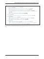
24.1 How to install the plugin manually? . . . . . . . . . . . . . . . . . . . . . . . . . . . . . . . . . 201
25 Pre processing
25.1 Which image bands should I use for a semi-automatic classification? . . . . . . . . . . . . .
25.2 Which Landsat bands can be converted to reflectance by the SCP? . . . . . . . . . . . . . . .
25.3 Can I apply the Landsat conversion and DOS correction to clipped bands? . . . . . . . . . . .
25.4 Can I apply the DOS correction to Landsat bands with black border (i.e. with NoData value)?
25.5 How to remove cloud cover from Landsat images? . . . . . . . . . . . . . . . . . . . . . . .
25.6 How do I create a virtual raster manually in QGIS? . . . . . . . . . . . . . . . . . . . . . . .
.
.
.
.
.
.
.
.
.
.
.
.
203
203
203
203
203
204
204
26 Tutorials
205
26.1 Why using only Landsat 8 band 10 in the estimation of surface temperature? . . . . . . . . . . . 205
iii
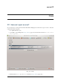
27 Errors
27.1 How can I report an error? . . . . . . . . . . . . . . . . . . . . . . . . .
27.2 Why am I having issues during the creation of the Landsat virtual raster?
27.3 Error [26] ‘The version of Numpy is outdated’. Why? . . . . . . . . . .
27.4 Error ‘Plugin is damaged. Python said: ascii’. Why? . . . . . . . . . . .
.
.
.
.
.
.
.
.
.
.
.
.
.
.
.
.
.
.
.
.
.
.
.
.
.
.
.
.
.
.
.
.
.
.
.
.
.
.
.
.
207
207
208
208
209
28 Other
28.1 What are free and valuable resources about remote sensing and GIS? . . . . . .
28.2 Where can I ask a new question? . . . . . . . . . . . . . . . . . . . . . . . . . .
28.3 Where can I find more tutorials about SCP, also in languages other than English?
28.4 How can I translate this user manual to another language? . . . . . . . . . . . .
.
.
.
.
.
.
.
.
.
.
.
.
.
.
.
.
.
.
.
.
.
.
.
.
.
.
.
.
.
.
.
.
.
.
.
.
211
211
211
211
212
iv
.
.
.
.
.
.
.
.
.
.
.
.
Semi-Automatic Classification Plugin Documentation, Release 4.8.0.1
Written by Luca Congedo, the Semi-Automatic Classification Plugin (SCP) is a free open source plugin for
QGIS that allows for the semi-automatic classification (also supervised classification) of remote sensing images.
Also, it provides several tools for the pre processing of images, the post processing of classifications, and the raster
calculation.
SCP allows for the rapid creation of ROIs (training areas), through region growing algorithm, which are stored
in a shapefile. The scatter plot or ROIs is available. Spectral signatures of training areas are calculated automatically, and can be displayed in a spectral signature plot along with the values thereof. Spectral distances among
signatures (e.g. Jeffries Matusita distance, or spectral angle) can be calculated for assessing spectral separability.
Spectral signatures can be exported and imported from external sources. Also, a tool allows for the selection and
download of spectral signatures from the USGS Spectral Library .
SCP implements a tool for searching and downloading Landsat and Sentinel images. The following tools are
available for the pre processing of images: automatic Landsat conversion to surface reflectance, clipping
multiple rasters, and splitting multi-band rasters.
The classification algorithms available are: Minimum Distance, Maximum Likelihood, Spectral Angle Mapping.
SCP allows for interactive preview of classification.
The post processing tools include: accuracy assessment, land cover change, classification report, classification
to vector, reclassification of raster values. Also, a band calc tool allows for the raster calculation using NumPy
functions .
For more information and tutorials visit the official site From GIS to Remote Sensing.
How to cite:
Congedo Luca, Munafo’ Michele, Macchi Silvia (2013). “Investigating the Relationship between Land Cover and
Vulnerability to Climate Change in Dar es Salaam”. Working Paper, Rome: Sapienza University. Available at:
http://www.planning4adaptation.eu/Docs/papers/08_NWP-DoM_for_LCC_in_Dar_using_Landsat_Imagery.pdf
License:
Except where otherwise noted, content of this work is licensed under a Creative Commons Attribution-ShareAlike
4.0 International License.
Semi-Automatic Classification Plugin is free software: you can
redistribute it and/or modify it under the terms of the GNU General Public
License as published by the Free Software Foundation, version 3 of the
License. Semi-Automatic Classification Plugin is distributed in the
hope that it will be useful, but WITHOUT ANY WARRANTY; without even the
implied warranty of MERCHANTABILITY or FITNESS FOR A PARTICULAR PURPOSE.
See the GNU General Public License for more details. You should have
received a copy of the GNU General Public License along with Semi-Automatic
Classification Plugin. If not, see http://www.gnu.org/licenses/.
The first version of the Semi-Automatic Classification Plugin was written
by Luca Congedo for the Adapting to Climate Change in Coastal Dar es Salaam
Project (http://www.planning4adaptation.eu).
Contents
1
Semi-Automatic Classification Plugin Documentation, Release 4.8.0.1
2
Contents
Part I
Plugin Installation
3
Semi-Automatic Classification Plugin Documentation, Release 4.8.0.1
The Semi-Automatic Classification Plugin requires the installation of GDAL, OGR, NumPy, SciPy and Matplotlib.
This chapter describes the installation of the Semi-Automatic Classification Plugin for the supported Operating
Systems.
5
Semi-Automatic Classification Plugin Documentation, Release 4.8.0.1
6
CHAPTER 1
Installation in Windows 32 bit
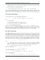
1.1 QGIS download and installation
• Download the latest QGIS version 32 bit from here (the direct download of QGIS 2.8 from this link);
• Execute the QGIS installer with administrative rights, accepting the default configuration.
Now, QGIS 2 is installed.
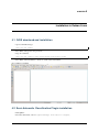
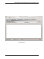
1.2 Semi-Automatic Classification Plugin installation
• Run QGIS 2;
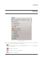
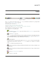
• From the main menu, select Plugins > Manage and Install Plugins;
• From the menu All, select the Semi-Automatic Classification Plugin and click the button Install
plugin;
7
Semi-Automatic Classification Plugin Documentation, Release 4.8.0.1
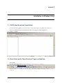
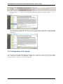
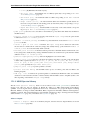
• The SCP should be automatically activated; however, be sure that the Semi-Automatic Classification Plugin is checked in the menu Installed (the restart of QGIS could be necessary to complete the SCP
installation);
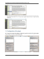
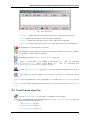
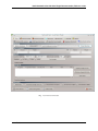
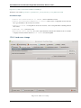
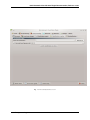
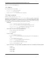
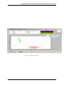
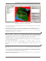
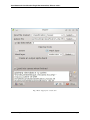
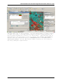
1.3 Configuration of the plugin
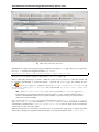
Now, the Semi-Automatic Classification Plugin is installed and two docks and a toolbar should be added to QGIS.
Also, a SCP menu is available in the Menu Bar of QGIS. It is possible to move the Toolbar (page 87) and the
docks according to your needs, as in the following image.
8
Chapter 1. Installation in Windows 32 bit
Semi-Automatic Classification Plugin Documentation, Release 4.8.0.1
1.4 Known issues
QGIS 32bit installation could include an old version of NumPy as default; in order to use some SCP tools (e.g.
Land cover change (page 120) ), the update of NumPy is required. Please, follow the instructions described in
Error [26] ‘The version of Numpy is outdated’. Why? (page 208).
1.4. Known issues
9
Semi-Automatic Classification Plugin Documentation, Release 4.8.0.1
10
Chapter 1. Installation in Windows 32 bit
CHAPTER 2
Installation in Windows 64 bit
2.1 QGIS download and installation
• Download the latest QGIS version 64 bit from here (the direct download of QGIS 2.8 from this link);
• Execute the QGIS installer with administrative rights, accepting the default configuration.
Now, QGIS 2 is installed.
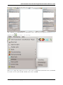
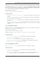
2.2 Semi-Automatic Classification Plugin installation
• Run QGIS 2;
• From the main menu, select Plugins > Manage and Install Plugins;
• From the menu All, select the Semi-Automatic Classification Plugin and click the button Install
plugin;
11
Semi-Automatic Classification Plugin Documentation, Release 4.8.0.1
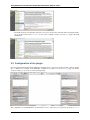
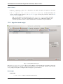
• The SCP should be automatically activated; however, be sure that the Semi-Automatic Classification Plugin is checked in the menu Installed (the restart of QGIS could be necessary to complete the SCP
installation);
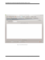
2.3 Configuration of the plugin
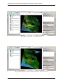
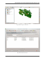
Now, the Semi-Automatic Classification Plugin is installed and two docks and a toolbar should be added to QGIS.
Also, a SCP menu is available in the Menu Bar of QGIS. It is possible to move the Toolbar (page 87) and the
docks according to your needs, as in the following image.
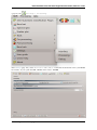
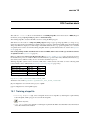
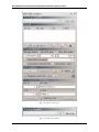
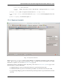
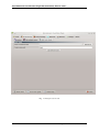
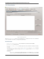
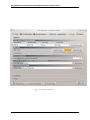
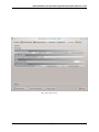
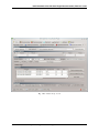
The configuration of available RAM is recommended in order to reduce the processing time. From the SCP menu
12
Chapter 2. Installation in Windows 64 bit
Semi-Automatic Classification Plugin Documentation, Release 4.8.0.1
(page 85) select
Settings > Processing .
In the Settings (page 129), set the Available RAM (MB) to a value that should be half of the system RAM.
For instance, if your system has 2GB of RAM, set the value to 1024MB.
2.3. Configuration of the plugin
13
Semi-Automatic Classification Plugin Documentation, Release 4.8.0.1
14
Chapter 2. Installation in Windows 64 bit
CHAPTER 3
Installation in Ubuntu Linux
3.1 QGIS download and installation
• Open a terminal and type:
sudo apt-get update
• Press Enter and type the user password;
• Type in a terminal:
sudo apt-get install qgis python-matplotlib python-scipy
• Press Enter and wait until the software is downloaded and installed.
Now, QGIS 2 is installed.
3.2 Semi-Automatic Classification Plugin installation
• Run QGIS 2;
• From the main menu, select Plugins > Manage and Install Plugins;
15
Semi-Automatic Classification Plugin Documentation, Release 4.8.0.1
• From the menu All, select the Semi-Automatic Classification Plugin and click the button Install
plugin;
• The SCP should be automatically activated; however, be sure that the Semi-Automatic Classification Plugin is checked in the menu Installed (the restart of QGIS could be necessary to complete the SCP
installation);
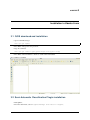
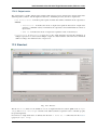
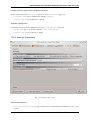
3.3 Configuration of the plugin
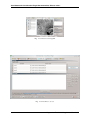
Now, the Semi-Automatic Classification Plugin is installed and two docks and a toolbar should be added to QGIS.
Also, a SCP menu is available in the Menu Bar of QGIS. It is possible to move the Toolbar (page 87) and the
docks according to your needs, as in the following image.
16
Chapter 3. Installation in Ubuntu Linux
Semi-Automatic Classification Plugin Documentation, Release 4.8.0.1
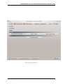
The configuration of available RAM is recommended in order to reduce the processing time. From the SCP menu
(page 85) select
Settings > Processing .
In the Settings (page 129), set the Available RAM (MB) to a value that should be half of the system RAM.
For instance, if your system has 2GB of RAM, set the value to 1024MB.
3.3. Configuration of the plugin
17
Semi-Automatic Classification Plugin Documentation, Release 4.8.0.1
18
Chapter 3. Installation in Ubuntu Linux
CHAPTER 4
Installation in Debian Linux
4.1 QGIS download and installation
• Open a terminal and type:
sudo apt-get update
• Press Enter and type the user password;
• Type in a terminal:
sudo apt-get install qgis python-matplotlib python-scipy
• Press Enter and wait until the software is downloaded and installed.
Now, QGIS 2 is installed.
4.2 Semi-Automatic Classification Plugin installation
• Run QGIS 2;
• From the main menu, select Plugins > Manage and Install Plugins;
19
Semi-Automatic Classification Plugin Documentation, Release 4.8.0.1
• From the menu All, select the Semi-Automatic Classification Plugin and click the button Install
plugin;
• The SCP should be automatically activated; however, be sure that the Semi-Automatic Classification Plugin is checked in the menu Installed (the restart of QGIS could be necessary to complete the SCP
installation);
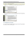
4.3 Configuration of the plugin
Now, the Semi-Automatic Classification Plugin is installed and two docks and a toolbar should be added to QGIS.
Also, a SCP menu is available in the Menu Bar of QGIS. It is possible to move the Toolbar (page 87) and the
docks according to your needs, as in the following image.
20
Chapter 4. Installation in Debian Linux
Semi-Automatic Classification Plugin Documentation, Release 4.8.0.1
The configuration of available RAM is recommended in order to reduce the processing time. From the SCP menu
(page 85) select
Settings > Processing .
In the Settings (page 129), set the Available RAM (MB) to a value that should be half of the system RAM.
For instance, if your system has 2GB of RAM, set the value to 1024MB.
4.3. Configuration of the plugin
21
Semi-Automatic Classification Plugin Documentation, Release 4.8.0.1
22
Chapter 4. Installation in Debian Linux
CHAPTER 5
Installation in Mac OS
5.1 QGIS download and installation
• Download and install the latest version of QGIS and GDAL from here .
• In addition, download and install the python modules Numpy, Scipy, and Matplotlib from this link .
Now, QGIS 2 is installed.
5.2 Semi-Automatic Classification Plugin installation
• Run QGIS 2;
• From the main menu, select Plugins > Manage and Install Plugins;
• From the menu All, select the Semi-Automatic Classification Plugin and click the button Install
plugin;
23
Semi-Automatic Classification Plugin Documentation, Release 4.8.0.1
• The SCP should be automatically activated; however, be sure that the Semi-Automatic Classification Plugin is checked in the menu Installed (the restart of QGIS could be necessary to complete the SCP
installation);
5.3 Configuration of the plugin
Now, the Semi-Automatic Classification Plugin is installed and two docks and a toolbar should be added to QGIS.
Also, a SCP menu is available in the Menu Bar of QGIS. It is possible to move the Toolbar (page 87) and the
docks according to your needs, as in the following image.
The configuration of available RAM is recommended in order to reduce the processing time. From the SCP menu
24
Chapter 5. Installation in Mac OS
Semi-Automatic Classification Plugin Documentation, Release 4.8.0.1
(page 85) select
Settings > Processing .
In the Settings (page 129), set the Available RAM (MB) to a value that should be half of the system RAM.
For instance, if your system has 2GB of RAM, set the value to 1024MB.
5.3. Configuration of the plugin
25
Semi-Automatic Classification Plugin Documentation, Release 4.8.0.1
26
Chapter 5. Installation in Mac OS
Part II
Brief Introduction to Remote Sensing
27
Semi-Automatic Classification Plugin Documentation, Release 4.8.0.1
• Basic Definitions (page 31)
– GIS definition (page 31)
– Remote Sensing definition (page 31)
– Sensors (page 33)
– Radiance and Reflectance (page 33)
– Spectral Signature (page 33)
– Landsat Satellite (page 34)
– Sentinel-2 Satellite (page 34)
– Color Composite (page 35)
– Pan-sharpening (page 35)
• Supervised Classification Definitions (page 39)
– Land Cover (page 39)
– Supervised Classification (page 39)
– Training Areas (page 39)
– Classes and Macroclasses (page 39)
– Classification Algorithms (page 40)
– Spectral Distance (page 42)
– Classification Result (page 44)
– Accuracy Assessment (page 44)
• Landsat image conversion to reflectance and DOS1 atmospheric correction (page 47)
– Radiance at the Sensor’s Aperture (page 47)
– Top Of Atmosphere (TOA) Reflectance (page 47)
– Surface Reflectance (page 48)
– DOS1 Correction (page 48)
• Conversion to At-Satellite Brightness Temperature (page 51)
29
Semi-Automatic Classification Plugin Documentation, Release 4.8.0.1
30
CHAPTER 6
Basic Definitions
This chapter provides basic definitions about GIS and remote sensing.
6.1 GIS definition
There are several definitions of GIS (Geographic Information Systems), which is not simply a program. In general,
GIS are systems that allow for the use of geographic information (data have spatial coordinates). In particular,
GIS allow for the view, query, calculation and analysis of spatial data, which are mainly distinguished in raster
or vector data structures. Vector is made of objects that can be points, lines or polygons, and each object can
have one ore more attribute values; a raster is a grid (or image) where each cell has an attribute value (Fisher and
Unwin, 2005). Several GIS applications use raster images that are derived from remote sensing.
6.2 Remote Sensing definition
A general definition of Remote Sensing is “the science and technology by which the characteristics of objects of
interest can be identified, measured or analyzed the characteristics without direct contact” (JARS, 1993).
Usually, remote sensing is the measurement of the energy that is emanated from the Earth’s surface. If the source
of the measured energy is the sun, then it is called passive remote sensing, and the result of this measurement can
be a digital image (Richards and Jia, 2006). If the measured energy is not emitted by the Sun but from the sensor
platform then it is defined as active remote sensing, such as radar sensors which work in the microwave range
(Richards and Jia, 2006).
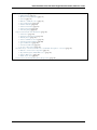
The electromagnetic spectrum is “the system that classifies, according to wavelength, all energy (from short
cosmic to long radio) that moves, harmonically, at the constant velocity of light” (NASA, 2013). Passive sensors
measure energy from the optical regions of the electromagnetic spectrum: visible, near infrared (i.e. IR), shortwave IR, and thermal IR (see Figure Electromagnetic-Spectrum (page 32)).
The interaction between solar energy and materials depends on the wavelength; solar energy goes from the Sun to
the Earth and then to the sensor. Along this path, solar energy is (NASA, 2013):
• Transmitted - The energy passes through with a change in velocity as determined by the index of refraction
for the two media in question.
• Absorbed - The energy is given up to the object through electron or molecular reactions.
• Reflected - The energy is returned unchanged with the angle of incidence equal to the angle of reflection. Reflectance is the ratio of reflected energy to that incident on a body. The wavelength reflected (not
absorbed) determines the color of an object.
• Scattered - The direction of energy propagation is randomly changed. Rayleigh and Mie scatter are the two
most important types of scatter in the atmosphere.
• Emitted - Actually, the energy is first absorbed, then re-emitted, usually at longer wavelengths. The object
heats up.
31
Semi-Automatic Classification Plugin Documentation, Release 4.8.0.1
Fig. 6.1: Electromagnetic-Spectrum
32
by Victor Blacus (SVG version of File:Electromagnetic-Spectrum.png)
Chapter 6. Basic Definitions
[CC-BY-SA-3.0 (http://creativecommons.org/licenses/by-sa/3.0)]
via Wikimedia Commons
http://commons.wikimedia.org/wiki/File%3AElectromagnetic-Spectrum.svg
Semi-Automatic Classification Plugin Documentation, Release 4.8.0.1
6.3 Sensors
Sensors can be on board of airplanes or on board of satellites, measuring the electromagnetic radiation at specific
ranges (usually called bands). As a result, the measures are quantized and converted into a digital image, where
each picture elements (i.e. pixel) has a discrete value in units of Digital Number (DN) (NASA, 2013). The
resulting images have different characteristics (resolutions) depending on the sensor. There are several kinds of
resolutions:
• Spatial resolution, usually measured in pixel size, “is the resolving power of an instrument needed for the
discrimination of features and is based on detector size, focal length, and sensor altitude” (NASA, 2013);
spatial resolution is also referred to as geometric resolution or IFOV;
• Spectral resolution, is the number and location in the electromagnetic spectrum (defined by two wavelengths) of the spectral bands (NASA, 2013) in multispectral sensors, for each band corresponds an image;
• Radiometric resolution, usually measured in bits (binary digits), is the range of available brightness values,
which in the image correspond to the maximum range of DNs; for example an image with 8 bit resolution
has 256 levels of brightness (Richards and Jia, 2006);
• For satellites sensors, there is also the temporal resolution, which is the time required for revisiting the
same area of the Earth (NASA, 2013).
6.4 Radiance and Reflectance
Sensors measure the radiance, which corresponds to the brightness in a given direction toward the sensor; it useful
to define also the reflectance as the ratio of reflected versus total power energy.
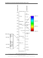
6.5 Spectral Signature
The spectral signature is the reflectance as a function of wavelength (see Figure Spectral Reflectance Curves
of Four Different Targets (page 33)); each material has a unique signature, therefore it can be used for material
classification (NASA, 2013).
Fig. 6.2: Spectral Reflectance Curves of Four Different Targets
(from NASA, 2013)
6.3. Sensors
33
Semi-Automatic Classification Plugin Documentation, Release 4.8.0.1
6.6 Landsat Satellite
Landsat is a set of multispectral satellites developed by the NASA (National Aeronautics and Space Administration of USA), since the early 1970’s.
Landsat images are very used for environmental research. The resolutions of Landsat 4 and Landsat 5 sensors
are reported in the following table (from http://landsat.usgs.gov/band_designations_landsat_satellites.php); also,
Landsat temporal resolution is 16 days (NASA, 2013).
Landsat 4, Landsat 5 Bands
Band 1 - Blue
Band 2 - Green
Band 3 - Red
Band 4 - Near Infrared (NIR)
Band 5 - SWIR
Band 6 - Thermal Infrared
Band 7 - SWIR
Wavelength [micrometers]
0.45 - 0.52
0.52 - 0.60
0.63 - 0.69
0.76 - 0.90
1.55 - 1.75
10.40 - 12.50
2.08 - 2.35
Resolution [meters]
30
30
30
30
30
120 (resampled to 30)
30
The resolutions of Landsat 7 sensor are reported in the following table (from
http://landsat.usgs.gov/band_designations_landsat_satellites.php); also, Landsat temporal resolution is 16
days (NASA, 2013).
Landsat 7 Bands
Band 1 - Blue
Band 2 - Green
Band 3 - Red
Band 4 - Near Infrared (NIR)
Band 5 - SWIR
Band 6 - Thermal Infrared
Band 7 - SWIR
Band 8 - Panchromatic
Wavelength [micrometers]
0.45 - 0.52
0.52 - 0.60
0.63 - 0.69
0.77 - 0.90
1.57 - 1.75
10.40 - 12.50
2.09 - 2.35
0.52 - 0.90
Resolution [meters]
30
30
30
30
30
60 (resampled to 30)
30
15
The resolutions of Landsat 8 sensor are reported in the following table (from
http://landsat.usgs.gov/band_designations_landsat_satellites.php); also, Landsat temporal resolution is 16
days (NASA, 2013).
Landsat 8 Bands
Band 1 - Coastal aerosol
Band 2 - Blue
Band 3 - Green
Band 4 - Red
Band 5 - Near Infrared (NIR)
Band 6 - SWIR 1
Band 7 - SWIR 2
Band 8 - Panchromatic
Band 9 - Cirrus
Band 10 - Thermal Infrared (TIRS) 1
Band 11 - Thermal Infrared (TIRS) 2
Wavelength [micrometers]
0.43 - 0.45
0.45 - 0.51
0.53 - 0.59
0.64 - 0.67
0.85 - 0.88
1.57 - 1.65
2.11 - 2.29
0.50 - 0.68
1.36 - 1.38
10.60 - 11.19
11.50 - 12.51
Resolution [meters]
30
30
30
30
30
30
30
15
30
100 (resampled to 30)
100 (resampled to 30)
A vast archive of images is freely available from the U.S. Geological Survey . For more information about how to
freely download Landsat images read this .
6.7 Sentinel-2 Satellite
Sentinel-2 is a multispectral satellite developed by the European Space Agency (ESA) in the frame of Copernicus
land monitoring services. Sentinel-2 acquires 13 spectral bands with the spatial resolution of 10m, 20m and 60m
depending on the band, as illustrated in the following table (ESA, 2015).
34
Chapter 6. Basic Definitions
Semi-Automatic Classification Plugin Documentation, Release 4.8.0.1
Sentinel-2 Bands
Band 1 - Coastal aerosol
Band 2 - Blue
Band 3 - Green
Band 4 - Red
Band 5 - Vegetation Red Edge
Band 6 - Vegetation Red Edge
Band 7 - Vegetation Red Edge
Band 8 - NIR
Band 8A - Vegetation Red Edge
Band 9 - Water vapour
Band 10 - SWIR - Cirrus
Band 11 - SWIR
Band 12 - SWIR
Central Wavelength [micrometers]
0.443
0.490
0.560
0.665
0.705
0.740
0.783
0.842
0.865
0.945
1.375
1.610
2.190
Resolution [meters]
60
10
10
10
20
20
20
10
20
60
60
20
20
Sentinel-2 images are freely available from the ESA website https://scihub.esa.int/dhus/ .
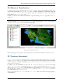
6.8 Color Composite
Often, a combination is created of three individual monochrome images, in which each is assigned a given color;
this is defined color composite and is useful for photo interpretation (NASA, 2013). Color composites are usually
expressed as:
“R G B = Br Bg Bb”
where:
• R stands for Red;
• G stands for Green;
• B stands for Blue;
• Br is the band number associated to the Red color;
• Bg is the band number associated to the Green color;
• Bb is the band number associated to the Blue color.
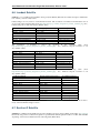
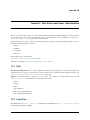
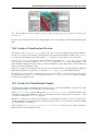
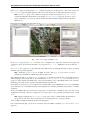
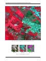
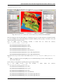
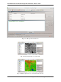
The following Figure Color composite of a Landsat 8 image (page 36) shows a color composite “R G B = 4 3 2”
of a Landsat 8 image (for Landsat 7 the same color composite is R G B = 3 2 1) and a color composite “R G B =
5 4 3” (for Landsat 7 the same color composite is R G B = 4 3 2). The composite “R G B = 5 4 3” is useful for
the interpretation of the image because vegetation pixels appear red (healthy vegetation reflects a large part of the
incident light in the near-infrared wavelength, resulting in higher reflectance values for band 5, thus higher values
for the associated color red).
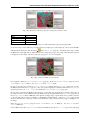
6.9 Pan-sharpening
Pan-sharpening is the combination of the spectral information of multispectral bands (MS), which have lower
spatial resolution (for Landsat bands, spatial resolution is 30m), with the spatial resolution of a panchromatic
band (PAN), which for Landsat 7 and 8 it is 15m. The result is a multispectral image with the spatial resolution
of the panchromatic band (e.g. 15m). In SCP, a Brovey Transform is applied, where the pan-sharpened values of
each multispectral band are calculated as (Johnson, Tateishi and Hoan, 2012):
𝑀 𝑆𝑝𝑎𝑛 = 𝑀 𝑆 * 𝑃 𝐴𝑁/𝐼
where 𝐼 is Intensity, which is a function of multispectral bands.
6.8. Color Composite
35
Semi-Automatic Classification Plugin Documentation, Release 4.8.0.1
Fig. 6.3: Color composite of a Landsat 8 image
Data available from the U.S. Geological Survey
The following weights for I are defined, basing on several tests performed using the SCP. For Landsat 8, Intensity
is calculated as:
𝐼 = (0.42 * 𝐵𝑙𝑢𝑒𝑏𝑎𝑛𝑑 + 0.98 * 𝐺𝑟𝑒𝑒𝑛𝑏𝑎𝑛𝑑 + 0.6 * 𝑅𝑒𝑑𝑏𝑎𝑛𝑑)/2
For Landsat 7, Intensity is calculated as:
𝐼 = (0.42 * 𝐵𝑙𝑢𝑒𝑏𝑎𝑛𝑑 + 0.98 * 𝐺𝑟𝑒𝑒𝑛𝑏𝑎𝑛𝑑 + 0.6 * 𝑅𝑒𝑑𝑏𝑎𝑛𝑑 + 𝑁 𝐼𝑅𝑏𝑎𝑛𝑑)/3
36
Chapter 6. Basic Definitions
Semi-Automatic Classification Plugin Documentation, Release 4.8.0.1
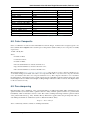
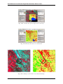
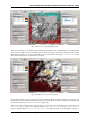
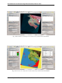
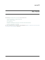
Fig. 6.4: Example of pan-sharpening of a Landsat 8 image. Left, original multispectral bands (30m); right,
pan-sharpened bands (15m)
Data available from the U.S. Geological Survey
6.9. Pan-sharpening
37
Semi-Automatic Classification Plugin Documentation, Release 4.8.0.1
38
Chapter 6. Basic Definitions
CHAPTER 7
Supervised Classification Definitions
This chapter provides basic definitions about supervised classifications.
7.1 Land Cover
Land cover is the material at the ground, such as soil, vegetation, water, asphalt, etc. (Fisher and Unwin, 2005).
Depending on the sensor resolutions, the number and kind of land cover classes that can be identified in the image
can vary significantly.
7.2 Supervised Classification
A semi-automatic classification (also supervised classification) is an image processing technique that allows
for the identification of materials in an image, according to their spectral signatures. There are several kinds of
classification algorithms, but the general purpose is to produce a thematic map of the land cover.
Image processing and GIS spatial analyses require specific software such as the Semi-Automatic Classification
Plugin for QGIS.
7.3 Training Areas
Usually, supervised classifications require the user to select one or more Regions of Interest (ROIs, also Training
Areas) for each land cover class identified in the image. ROIs are polygons drawn over homogeneous areas of the
image that overlay pixels belonging to the same land cover class.
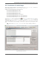
7.4 Classes and Macroclasses
Land cover classes are identified with an arbitrary ID code (i.e. Identifier). SCP allows for the definition of
Macroclass ID (i.e. MC ID) and Class ID (i.e. C ID), which are the identification codes of land cover classes.
A Macroclass is a group of ROIs having different Class ID, which is useful when one needs to classify materials
that have different spectral signatures in the same land cover class. For instance, one can identify grass (e.g. ID
class = 1 and Macroclass ID = 1 ) and trees (e.g. ID class = 2 and Macroclass ID = 1 ) as
vegetation class (e.g. Macroclass ID = 1 ). Multiple Class IDs can be assigned to the same Macroclass ID,
but the same Class ID cannot be assigned to multiple Macroclass IDs, as shown in the following table.
Macroclass name
Vegetation
Vegetation
Built-up
Macroclass ID
1
1
2
Class name
Grass
Trees
Road
Class ID
1
2
3
39
Semi-Automatic Classification Plugin Documentation, Release 4.8.0.1
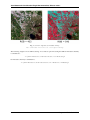
Therefore, Classes are subsets of a Macroclass as illustrated in Figure Macroclass example (page 40).
Fig. 7.1: Macroclass example
If the use of Macroclass is not required for the study purpose, then the same Macroclass ID can be defined for all
the ROIs (e.g. Macroclass ID = 1) and Macroclass values are ignored in the classification process.
7.5 Classification Algorithms
The spectral signatures (spectral characteristics) of reference land cover classes are calculated considering the
values of pixels under each ROI having the same Class ID (or Macroclass ID). Therefore, the classification algorithm classifies the whole image by comparing the spectral characteristics of each pixel to the spectral characteristics of reference land cover classes. SCP implements the following classification algorithms.
7.5.1 Minimum Distance
Minimum Distance algorithm calculates the Euclidean distance 𝑑(𝑥, 𝑦) between spectral signatures of image pixels
and training spectral signatures, according to the following equation:
⎯
⎸ 𝑛
⎸∑︁
𝑑(𝑥, 𝑦) = ⎷ (𝑥𝑖 − 𝑦𝑖 )2
𝑖=1
where:
• 𝑥 = spectral signature vector of an image pixel;
• 𝑦 = spectral signature vector of a training area;
40
Chapter 7. Supervised Classification Definitions
Semi-Automatic Classification Plugin Documentation, Release 4.8.0.1
• 𝑛 = number of image bands.
Therefore, the distance is calculated for every pixel in the image, assigning the class of the spectral signature that
is closer, according to the following discriminant function (adapted from Richards and Jia, 2006):
𝑥 ∈ 𝐶𝑘 ⇐⇒ 𝑑(𝑥, 𝑦𝑘 ) < 𝑑(𝑥, 𝑦𝑗 )∀𝑘 ̸= 𝑗
where:
• 𝐶𝑘 = land cover class 𝑘;
• 𝑦𝑘 = spectral signature of class 𝑘;
• 𝑦𝑗 = spectral signature of class 𝑗.
It is possible to define a threshold 𝑇𝑖 in order to exclude pixels below this value from the classification:
𝑥 ∈ 𝐶𝑘 ⇐⇒ 𝑑(𝑥, 𝑦𝑘 ) < 𝑑(𝑥, 𝑦𝑗 )∀𝑘 ̸= 𝑗
𝑎𝑛𝑑
𝑑(𝑥, 𝑦𝑘 ) < 𝑇𝑖
7.5.2 Maximum Likelihood
Maximum Likelihood algorithm calculates the probability distributions for the classes, related to Bayes’ theorem,
estimating if a pixel belongs to a land cover class. In particular, the probability distributions for the classes are
assumed the of form of multivariate normal models (Richards & Jia, 2006). In order to use this algorithm, a
sufficient number of pixels is required for each training area allowing for the calculation of the covariance matrix.
The discriminant function, described by Richards and Jia (2006), is calculated for every pixel as:
𝑔𝑘 (𝑥) = ln 𝑝(𝐶𝑘 ) −
1
1
ln |Σ𝑘 | − (𝑥 − 𝑦𝑘 )𝑡 Σ−1
𝑘 (𝑥 − 𝑦𝑘 )
2
2
where:
• 𝐶𝑘 = land cover class 𝑘;
• 𝑥 = spectral signature vector of a image pixel;
• 𝑝(𝐶𝑘 ) = probability that the correct class is 𝐶𝑘 ;
• |Σ𝑘 | = determinant of the covariance matrix of the data in class 𝐶𝑘 ;
• Σ−1
𝑘 = inverse of the covariance matrix;
• 𝑦𝑘 = spectral signature vector of class 𝑘.
Therefore:
𝑥 ∈ 𝐶𝑘 ⇐⇒ 𝑔𝑘 (𝑥) > 𝑔𝑗 (𝑥)∀𝑘 ̸= 𝑗
In addition, it is possible to define a threshold to the discriminant function in order to exclude pixels below this
value from the classification. Considering a threshold 𝑇𝑖 the classification condition becomes:
𝑥 ∈ 𝐶𝑘 ⇐⇒ 𝑔𝑘 (𝑥) > 𝑔𝑗 (𝑥)∀𝑘 ̸= 𝑗
𝑎𝑛𝑑
𝑔𝑘 (𝑥) > 𝑇𝑖
Maximum likelihood is one of the most common supervised classifications, however the classification process can
be slower than Minimum Distance (page 40).
7.5. Classification Algorithms
41
Semi-Automatic Classification Plugin Documentation, Release 4.8.0.1
7.5.3 Spectra Angle Mapping
The Spectral Angle Mapping calculates the spectral angle between spectral signatures of image pixels and training
spectral signatures. The spectral angle 𝜃 is defined as (Kruse et al., 1993):
(︃
)︃
∑︀𝑛
𝑥
𝑦
𝑖
𝑖
𝑖=1
𝜃(𝑥, 𝑦) = cos−1
1
1
∑︀𝑛
∑︀𝑛
( 𝑖=1 𝑥2𝑖 ) 2 * ( 𝑖=1 𝑦𝑖2 ) 2
Where:
• 𝑥 = spectral signature vector of an image pixel;
• 𝑦 = spectral signature vector of a training area;
• 𝑛 = number of image bands.
Therefore a pixel belongs to the class having the lowest angle, that is:
𝑥 ∈ 𝐶𝑘 ⇐⇒ 𝜃(𝑥, 𝑦𝑘 ) < 𝜃(𝑥, 𝑦𝑗 )∀𝑘 ̸= 𝑗
where:
• 𝐶𝑘 = land cover class 𝑘;
• 𝑦𝑘 = spectral signature of class 𝑘;
• 𝑦𝑗 = spectral signature of class 𝑗.
In order to exclude pixels below this value from the classification it is possible to define a threshold 𝑇𝑖 :
𝑥 ∈ 𝐶𝑘 ⇐⇒ 𝜃(𝑥, 𝑦𝑘 ) < 𝜃(𝑥, 𝑦𝑗 )∀𝑘 ̸= 𝑗
𝑎𝑛𝑑
𝜃(𝑥, 𝑦𝑘 ) < 𝑇𝑖
Spectral Angle Mapping is largely used, especially with hyperspectral data.
7.6 Spectral Distance
It is useful to evaluate the spectral distance (or separability) between training signatures or pixels, in order to
assess if different classes that are too similar could cause classification errors. The SCP implements the following
algorithms for assessing similarity of spectral signatures.
7.6.1 Jeffries-Matusita Distance
Jeffries-Matusita Distance calculates the separability of a pair of probability distributions. This can be particularly
meaningful for evaluating the results of Maximum Likelihood (page 41) classifications.
The Jeffries-Matusita Distance 𝐽𝑥𝑦 is calculated as (Richards and Jia, 2006):
(︀
)︀
𝐽𝑥𝑦 = 2 1 − 𝑒−𝐵
where:
1
𝐵 = (𝑥 − 𝑦)𝑡
8
(︂
Σ𝑥 + Σ 𝑦
2
)︂−1
1
(𝑥 − 𝑦) + ln
2
(︃
|
)︃
Σ𝑥 +Σ𝑦
|
2
1
1
|Σ𝑥 | 2 |Σ𝑦 | 2
where:
• 𝑥 = first spectral signature vector;
• 𝑦 = second spectral signature vector;
42
Chapter 7. Supervised Classification Definitions
Semi-Automatic Classification Plugin Documentation, Release 4.8.0.1
• Σ𝑥 = covariance matrix of sample 𝑥;
• Σ𝑦 = covariance matrix of sample 𝑦;
The Jeffries-Matusita Distance is asymptotic to 2 when signatures are completely different, and tends to 0 when
signatures are identical.
7.6.2 Spectral Angle
The Spectral Angle is the most appropriate for assessing the Spectra Angle Mapping (page 42) algorithm. The
spectral angle 𝜃 is defined as (Kruse et al., 1993):
)︃
(︃
∑︀𝑛
−1
𝑖=1 𝑥𝑖 𝑦𝑖
𝜃(𝑥, 𝑦) = cos
1
1
∑︀𝑛
∑︀𝑛
( 𝑖=1 𝑥2𝑖 ) 2 * ( 𝑖=1 𝑦𝑖2 ) 2
Where:
• 𝑥 = spectral signature vector of an image pixel;
• 𝑦 = spectral signature vector of a training area;
• 𝑛 = number of image bands.
Spectral angle goes from 0 when signatures are identical to 90 when signatures are completely different.
7.6.3 Euclidean Distance
The Euclidean Distance is particularly useful for the evaluating the result of Minimum Distance (page 40) classifications. In fact, the distance is defined as:
⎯
⎸ 𝑛
⎸∑︁
𝑑(𝑥, 𝑦) = ⎷ (𝑥𝑖 − 𝑦𝑖 )2
𝑖=1
where:
• 𝑥 = first spectral signature vector;
• 𝑦 = second spectral signature vector;
• 𝑛 = number of image bands.
The Euclidean Distance is 0 when signatures are identical and tends to increase according to the spectral distance
of signatures.
7.6.4 Bray-Curtis Similarity
The Bray-Curtis Similarity is a statistic used for assessing the relationship between two samples (read this). It is
useful in general for assessing the similarity of spectral signatures, and Bray-Curtis Similarity 𝑆(𝑥, 𝑦) is calculated
as:
)︂
(︂ ∑︀𝑛
|(𝑥𝑖 − 𝑦𝑖 )|
∑︀𝑛
* 100
𝑆(𝑥, 𝑦) = 100 − ∑︀𝑛 𝑖=1
𝑖=1 𝑥𝑖 +
𝑖=1 𝑦𝑖
where:
• 𝑥 = first spectral signature vector;
• 𝑦 = second spectral signature vector;
• 𝑛 = number of image bands.
The Bray-Curtis similarity is calculated as percentage and ranges from 0 when signatures are completely different
to 100 when spectral signatures are identical.
7.6. Spectral Distance
43
Semi-Automatic Classification Plugin Documentation, Release 4.8.0.1
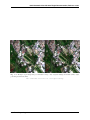
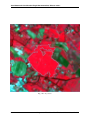
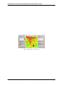
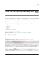
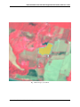
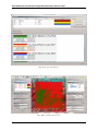
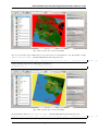
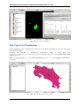
7.7 Classification Result
The result of the classification process is a raster (see an example of Landsat classification in Figure Landsat
classification (page 44)), where pixel values correspond to class IDs and each color represent a land cover class.
Fig. 7.2: Landsat classification
Data available from the U.S. Geological Survey
A certain amount of errors can occur in the land cover classification (i.e. pixels assigned to a wrong land cover
class), due to spectral similarity of classes, or wrong class definition during the ROI collection.
7.8 Accuracy Assessment
After the classification process, it is useful to assess the accuracy of land cover classification, in order to identify
and measure map errors. Usually, accuracy assessment is performed with the calculation of an error matrix,
which is a table that compares map information with reference data (i.e. ground truth data) for a number of
sample areas (Congalton and Green, 2009).
The following table is a scheme of error matrix, where k is the number of classes identified in the land cover
classification, and n is the total number of collected sample units. The items in the major diagonal (aii) are the
number of samples correctly identified, while the other items are classification error.
Class 1
Class 2
...
Class k
Total
Ground truth 1
𝑎11
𝑎21
...
𝑎𝑘1
𝑎+1
Ground truth 2
𝑎12
𝑎22
...
𝑎𝑘2
𝑎+2
...
...
...
...
...
...
Ground truth k
𝑎1𝑘
𝑎2𝑘
...
𝑎𝑘𝑘
𝑎+𝑘
Total
𝑎1+
𝑎2+
...
𝑎𝑘+
𝑛
Therefore, it is possible to calculate the overall accuracy as the ratio between the number of samples that are
correctly classified (the sum of the major diagonal), and the total number of sample units n (Congalton and Green,
2009).
For further information, the following documentation is freely available: Landsat 7 Science Data User’s Handbook, Remote Sensing Note , or Wikipedia.
References
• Congalton, R. and Green, K., 2009. Assessing the Accuracy of Remotely Sensed Data: Principles and
Practices. Boca Raton, FL: CRC Press.
• ESA, 2015. Sentinel-2 User Handbook. Available at https://sentinel.esa.int/documents/247904/685211/Sentinel2_User_Handbook
• Fisher, P. F. and Unwin, D. J., eds. 2005. Representing GIS. Chichester, England: John Wiley & Sons.
• JARS, 1993.
Remote Sensing Note.
http://www.jars1974.net/pdf/rsnote_e.html
44
Japan Association on Remote Sensing.
Available at
Chapter 7. Supervised Classification Definitions
Semi-Automatic Classification Plugin Documentation, Release 4.8.0.1
• Johnson, B. A., Tateishi, R. and Hoan, N. T., 2012. Satellite Image Pansharpening Using a Hybrid Approach
for Object-Based Image Analysis ISPRS International Journal of Geo-Information, 1, 228. Available at
http://www.mdpi.com/2220-9964/1/3/228)
• Kruse, F. A., et al., 1993. The Spectral Image Processing System (SIPS) - Interactive Visualization and
Analysis of Imaging spectrometer. Data Remote Sensing of Environment.
• NASA, 2013. Landsat 7 Science Data User’s Handbook. Available at http://landsathandbook.gsfc.nasa.gov
• Richards, J. A. and Jia, X., 2006. Remote Sensing Digital Image Analysis: An Introduction. Berlin,
Germany: Springer.
7.8. Accuracy Assessment
45
Semi-Automatic Classification Plugin Documentation, Release 4.8.0.1
46
Chapter 7. Supervised Classification Definitions
CHAPTER 8
Landsat image conversion to reflectance and DOS1 atmospheric
correction
This chapter provides information about the Landsat conversion to reflectance implemented in SCP Landsat
(page 114).
Landsat images downloaded from http://earthexplorer.usgs.gov or through the SCP tool Download Landsat
(page 108) are composed of several bands and a metadata file (MTL) which contains useful information about
image data.
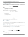
8.1 Radiance at the Sensor’s Aperture
Radiance is the “flux of energy (primarily irradiant or incident energy) per solid angle leaving a unit surface area
in a given direction”, “Radiance is what is measured at the sensor and is somewhat dependent on reflectance”
(NASA, 2011, p. 47).
The Spectral Radiance at the sensor’s aperture (𝐿𝜆 ) is measured in [watts/(meter squared * ster * 𝜇𝑚)] and for
Landsat images it is given by (https://landsat.usgs.gov/Landsat8_Using_Product.php):
𝐿𝜆 = 𝑀𝐿 * 𝑄𝑐𝑎𝑙 + 𝐴𝐿
where:
• 𝑀𝐿 = Band-specific multiplicative rescaling
ANCE_MULT_BAND_x, where x is the band number)
factor
from
Landsat
metadata
(RADI-
• 𝐴𝐿 = Band-specific additive rescaling factor from Landsat metadata (RADIANCE_ADD_BAND_x, where
x is the band number)
• 𝑄𝑐𝑎𝑙 = Quantized and calibrated standard product pixel values (DN)
8.2 Top Of Atmosphere (TOA) Reflectance
“For relatively clear Landsat scenes, a reduction in between-scene variability can be achieved through a normalization for solar irradiance by converting spectral radiance, as calculated above, to planetary reflectance or
albedo. This combined surface and atmospheric reflectance of the Earth is computed with the following formula” (NASA, 2011, p. 119):
𝜌𝑝 = (𝜋 * 𝐿𝜆 * 𝑑2 )/(𝐸𝑆𝑈 𝑁𝜆 * 𝑐𝑜𝑠𝜃𝑠 )
where:
• 𝜌𝑝 = Unitless TOA reflectance, which is “the ratio of reflected versus total power energy” (NASA, 2011, p.
47)
• 𝐿𝜆 = Spectral radiance at the sensor’s aperture (at-satellite radiance)
47
Semi-Automatic Classification Plugin Documentation, Release 4.8.0.1
• 𝑑 = Earth-Sun distance in astronomical units (provided with Landsat 8 metafile, and an excel file is available
from http://landsathandbook.gsfc.nasa.gov/excel_docs/d.xls)
• 𝐸𝑆𝑈 𝑁𝜆 = Mean solar exo-atmospheric irradiances
• 𝜃𝑠 = Solar zenith angle in degrees, which is equal to 𝜃𝑠 = 90° - 𝜃𝑒 where 𝜃𝑒 is the Sun elevation
It is worth pointing out that Landsat 8 images are provided with band-specific rescaling factors that allow for the
direct conversion from DN to TOA reflectance. However, the effects of the atmosphere (i.e. a disturbance on the
reflectance that varies with the wavelength) should be considered in order to measure the reflectance at the ground.
8.3 Surface Reflectance
As described by Moran et al. (1992), the land surface reflectance (𝜌) is:
𝜌 = [𝜋 * (𝐿𝜆 − 𝐿𝑝 ) * 𝑑2 ]/[𝑇𝑣 * ((𝐸𝑆𝑈 𝑁𝜆 * 𝑐𝑜𝑠𝜃𝑠 * 𝑇𝑧 ) + 𝐸𝑑𝑜𝑤𝑛 )]
where:
• 𝐿𝑝 is the path radiance
• 𝑇𝑣 is the atmospheric transmittance in the viewing direction
• 𝑇𝑧 is the atmospheric transmittance in the illumination direction
• 𝐸𝑑𝑜𝑤𝑛 is the downwelling diffuse irradiance
Therefore, we need several atmospheric measurements in order to calculate 𝜌 (physically-based corrections).
Alternatively, it is possible to use image-based techniques for the calculation of these parameters, without in-situ
measurements during image acquisition. It is worth mentioning that Landsat Surface Reflectance High Level Data
Products for Landsat 8 are available (for more information read http://landsat.usgs.gov/CDR_LSR.php).
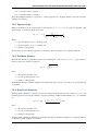
8.4 DOS1 Correction
The Dark Object Subtraction (DOS) is a family of image-based atmospheric corrections. Chavez (1996) explains
that “the basic assumption is that within the image some pixels are in complete shadow and their radiances received
at the satellite are due to atmospheric scattering (path radiance). This assumption is combined with the fact that
very few targets on the Earth’s surface are absolute black, so an assumed one-percent minimum reflectance is
better than zero percent”. It is worth pointing out that the accuracy of image-based techniques is generally lower
than physically-based corrections, but they are very useful when no atmospheric measurements are available as
they can improve the estimation of land surface reflectance. The path radiance is given by (Sobrino, et al., 2004):
𝐿𝑝 = 𝐿𝑚𝑖𝑛 − 𝐿𝐷𝑂1%
where:
• 𝐿𝑚𝑖𝑛 = “radiance that corresponds to a digital count value for which the sum of all the pixels with digital
counts lower or equal to this value is equal to the 0.01% of all the pixels from the image considered”
(Sobrino, et al., 2004, p. 437), therefore the radiance obtained with that digital count value (𝐷𝑁𝑚𝑖𝑛 )
• 𝐿𝐷𝑂1% = radiance of Dark Object, assumed to have a reflectance value of 0.01
Therfore for Landsat images:
𝐿𝑚𝑖𝑛 = 𝑀𝐿 * 𝐷𝑁𝑚𝑖𝑛 + 𝐴𝐿
The radiance of Dark Object is given by (Sobrino, et al., 2004):
𝐿𝐷𝑂1% = 0.01 * [(𝐸𝑆𝑈 𝑁𝜆 * 𝑐𝑜𝑠𝜃𝑠 * 𝑇𝑧 ) + 𝐸𝑑𝑜𝑤𝑛 ] * 𝑇𝑣 /(𝜋 * 𝑑2 )
Therefore the path radiance is:
𝐿𝑝 = 𝑀𝐿 * 𝐷𝑁𝑚𝑖𝑛 + 𝐴𝐿 − 0.01 * [(𝐸𝑆𝑈 𝑁𝜆 * 𝑐𝑜𝑠𝜃𝑠 * 𝑇𝑧 ) + 𝐸𝑑𝑜𝑤𝑛 ] * 𝑇𝑣 /(𝜋 * 𝑑2 )
48
Chapter 8. Landsat image conversion to reflectance and DOS1 atmospheric correction
Semi-Automatic Classification Plugin Documentation, Release 4.8.0.1
There are several DOS techniques (e.g. DOS1, DOS2, DOS3, DOS4), based on different assumption about 𝑇𝑣 ,
𝑇𝑧 , and 𝐸𝑑𝑜𝑤𝑛 . The simplest technique is the DOS1, where the following assumptions are made (Moran et al.,
1992):
• 𝑇𝑣 = 1
• 𝑇𝑧 = 1
• 𝐸𝑑𝑜𝑤𝑛 = 0
Therefore the path radiance is:
𝐿𝑝 = 𝑀𝐿 * 𝐷𝑁𝑚𝑖𝑛 + 𝐴𝐿 − 0.01 * 𝐸𝑆𝑈 𝑁𝜆 * 𝑐𝑜𝑠𝜃𝑠 /(𝜋 * 𝑑2 )
And the resulting land surface reflectance is given by:
𝜌 = [𝜋 * (𝐿𝜆 − 𝐿𝑝 ) * 𝑑2 ]/(𝐸𝑆𝑈 𝑁𝜆 * 𝑐𝑜𝑠𝜃𝑠 )
ESUN [W /(m2 * 𝜇𝑚)] values for Landsat sensors are provided in the following table.
Band
1
2
3
4
5
7
Landsat 4*
1957
1825
1557
1033
214.9
80.72
Landsat 5**
1983
1769
1536
1031
220
83.44
Landsat 7**
1997
1812
1533
1039
230.8
84.90
* from Chander & Markham (2003)
** from Finn, et al. (2012)
For Landsat 8, 𝐸𝑆𝑈 𝑁 can be calculated as (from http://grass.osgeo.org/grass65/manuals/i.landsat.toar.html):
𝐸𝑆𝑈 𝑁 = (𝜋 * 𝑑2 ) * 𝑅𝐴𝐷𝐼𝐴𝑁 𝐶𝐸_𝑀 𝐴𝑋𝐼𝑀 𝑈 𝑀/𝑅𝐸𝐹 𝐿𝐸𝐶𝑇 𝐴𝑁 𝐶𝐸_𝑀 𝐴𝑋𝐼𝑀 𝑈 𝑀
where RADIANCE_MAXIMUM and REFLECTANCE_MAXIMUM are provided by image metadata.
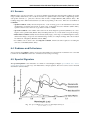
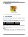
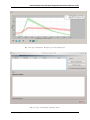
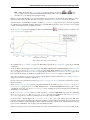
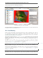
An example of comparison of to TOA reflectance, DOS1 corrected reflectance and the Landsat Surface Reflectance
High Level Data Products (ground truth) is provided in Figure Spectral signatures of a built-up pixel (page 49).
Fig. 8.1: Spectral signatures of a built-up pixel
Comparison of TOA reflectance, DOS1 corrected reflectance and Landsat Surface
Reflectance High Level Data Products
References
• Chander, G. & Markham, B. 2003. Revised Landsat-5 TM radiometric calibration procedures and postcalibration dynamic ranges Geoscience and Remote Sensing, IEEE Transactions on, 41, 2674 - 2677
8.4. DOS1 Correction
49
Semi-Automatic Classification Plugin Documentation, Release 4.8.0.1
• Chavez, P. S. 1996. Image-Based Atmospheric Corrections - Revisited and Improved Photogrammetric
Engineering and Remote Sensing, [Falls Church, Va.] American Society of Photogrammetry, 62, 10251036
• Finn, M.P., Reed, M.D, and Yamamoto, K.H. 2012.
A Straight Forward Guide for Processing Radiance and Reflectance for EO-1 ALI, Landsat 5 TM, Landsat 7 ETM+, and ASTER.
Unpublished Report from USGS/Center of Excellence for Geospatial Information Science, 8 p,
http://cegis.usgs.gov/soil_moisture/pdf/A%20Straight%20Forward%20guide%20for%20Processing%20Radiance%20and%2
• Moran, M.; Jackson, R.; Slater, P. & Teillet, P. 1992. Evaluation of simplified procedures for retrieval of
land surface reflectance factors from satellite sensor output Remote Sensing of Environment, 41, 169-184
• NASA (Ed.)
2011.
Landsat 7 Science Data Users Handbook Landsat Project
Science
Office
at
NASA’s
Goddard
Space
Flight
Center
in
Greenbelt,
186
http://landsathandbook.gsfc.nasa.gov/pdfs/Landsat7_Handbook.pdf
• Sobrino, J.; Jiménez-Muñoz, J. C. & Paolini, L. 2004. Land surface temperature retrieval from LANDSAT
TM 5 Remote Sensing of Environment, Elsevier, 90, 434-440
50
Chapter 8. Landsat image conversion to reflectance and DOS1 atmospheric correction
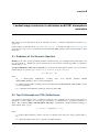
CHAPTER 9
Conversion to At-Satellite Brightness Temperature
This chapter provides information about the Landsat conversion to At-Satellite Brightness Temperature implemented in SCP Landsat (page 114). For information about how to estimate surface temperature read this post
.
For Landsat thermal bands, the conversion of DN to At-Satellite Brightness Temperature is given by (from
https://landsat.usgs.gov/Landsat8_Using_Product.php):
𝑇𝐵 = 𝐾2 /𝑙𝑛[(𝐾1 /𝐿𝜆 ) + 1]
where:
• 𝐾1 = Band-specific thermal conversion constant (in watts/meter squared * ster * 𝜇𝑚)
• 𝐾2 = Band-specific thermal conversion constant (in kelvin)
and 𝐿𝜆 is the Spectral Radiance at the sensor’s aperture, measured in watts/(meter squared * ster * 𝜇𝑚); for
Landsat images it is given by (from https://landsat.usgs.gov/Landsat8_Using_Product.php):
𝐿𝜆 = 𝑀𝐿 * 𝑄𝑐𝑎𝑙 + 𝐴𝐿
where:
• 𝑀𝐿 = Band-specific multiplicative rescaling
ANCE_MULT_BAND_x, where x is the band number)
factor
from
Landsat
metadata
(RADI-
• 𝐴𝐿 = Band-specific additive rescaling factor from Landsat metadata (RADIANCE_ADD_BAND_x, where
x is the band number)
• 𝑄𝑐𝑎𝑙 = Quantized and calibrated standard product pixel values (DN)
The 𝐾1 and 𝐾2 constant for Landsat sensors are provided in the following table:
Constant
𝐾1 (watts/meter squared * ster * 𝜇𝑚)
𝐾2 (Kelvin)
Landsat 4*
671.62
1284.30
Landsat 5*
607.76
1260.56
Landsat 7**
666.09
1282.71
* from Chander & Markham (2003)
** from NASA (2011)
For Landsat 8, the 𝐾1 and 𝐾2 values are provided in the image metafile.
References
• Chander, G. & Markham, B. 2003. Revised Landsat-5 TM radiometric calibration procedures and postcalibration dynamic ranges Geoscience and Remote Sensing, IEEE Transactions on, 41, 2674 - 2677
• NASA (Ed.)
2011.
Landsat 7 Science Data Users Handbook Landsat Project
Science
Office
at
NASA’s
Goddard
Space
Flight
Center
in
Greenbelt,
186
http://landsathandbook.gsfc.nasa.gov/pdfs/Landsat7_Handbook.pdf
51
Semi-Automatic Classification Plugin Documentation, Release 4.8.0.1
52
Chapter 9. Conversion to At-Satellite Brightness Temperature
Part III
Basic Tutorials
53
Semi-Automatic Classification Plugin Documentation, Release 4.8.0.1
Following, the list of basic tutorials that guide you through the steps of a land cover classification:
• Tutorial 1: Your First Land Cover Classification (page 57)
– Data (page 57)
– Load Data (page 57)
– Set the Input Image in SCP (page 58)
– Create the Training Shapefile and Signature List File (page 58)
– Create the ROIs (page 58)
– Create a Classification Preview (page 61)
– Create the Classification Output (page 61)
• Tutorial 2: Land Cover Classification of Landsat Images (page 65)
– Data Download (page 65)
– Automatic Conversion to Surface Reflectance (page 66)
– Clip Data (page 69)
– Create the Band Set (page 71)
– Open the Training Shapefile and Signature List File (page 71)
– Create the ROIs (page 73)
– Create a Classification Preview (page 78)
– Assess Spectral Signatures (page 78)
– Create the Classification Output (page 79)
• Other Tutorials (page 81)
55
Semi-Automatic Classification Plugin Documentation, Release 4.8.0.1
56
CHAPTER 10
Tutorial 1: Your First Land Cover Classification
This is a basic tutorial about the use of the Semi-Automatic Classification Plugin (SCP) for the classification
of a generic image. It is worth noticing that the image is multi-spectral. It is recommended to read the Brief
Introduction to Remote Sensing (page 29) before this tutorial.
In this tutorial we are going to classify a remote sensing image acquired over Frascati (Rome, Italy) in order to
identify the following land cover classes:
1. Water;
2. Built-up;
3. Vegetation;
4. Bare soil.
Following the video of this tutorial.
http://www.youtube.com/watch?v=nZffzX_sMnk
Alternative video link https://archive.org/details/video_basic_tutorial_1
10.1 Data
Download the image data from here (data available from the U.S. Geological Survey). It is a Landsat image, but
in this tutorial we are going to use this raster as a generic dataset. For a specific tutorial about Landsat images read
Tutorial 2: Land Cover Classification of Landsat Images (page 65) .
Unzip the downloaded file in a directory of your choice. The dataset is a multi-spectral raster (the file
sample_image.tif ) that includes the following Landsat bands:
1. Blue;
2. Green;
3. Red;
4. Near-Infrared;
5. Short Wavelength Infrared 1;
6. Short Wavelength Infrared 2.
10.2 Load Data
Start QGIS and load sample_image.tif in QGIS (from the QGIS menu Layer > Add Raster Layer
). The image is displayed in QGIS.
57
Semi-Automatic Classification Plugin Documentation, Release 4.8.0.1
Fig. 10.1: Image loaded in QGIS
10.3 Set the Input Image in SCP
In the SCP Toolbar (page 87) click the button
image select sample_image .
for refreshing the list Input image . In the list Input
In the list RGB select the item 4-3-2 for displaying a Color Composite (page 35) of Near-Infrared, Red, and
Green. The image in QGIS will be updated accordingly.
Fig. 10.2: Color composite RGB=4-3-2 of Input image
10.4 Create the Training Shapefile and Signature List File
In order to collect Training Areas (page 39) (ROIs) and calculate the Spectral Signature (page 33) thereof, we
need to create the Training shapefile and Signature list file in SCP.
In the ROI Creation dock (page 89) click the button New shp and define a name (e.g. ROI.shp ) in order to
create the Training shapefile that will store ROI polygons. The shapefile is created and added to QGIS.
The name of the Training shapefile is displayed in Training shapefile (page 89) .
Also, click the button Save in the Classification dock (page 95) and define a name (e.g. SIG.xml ) in order
to create the Signature list file that will store spectral signatures. The path of the Signature list
file is displayed in Signature list file (page 95) .
10.5 Create the ROIs
We are going to create ROIs defining the Classes and Macroclasses (page 39) . The Macroclass ID codes are
illustrated in the following table (of course, one can define different codes and classes according to the needs).
58
Chapter 10. Tutorial 1: Your First Land Cover Classification
Semi-Automatic Classification Plugin Documentation, Release 4.8.0.1
Fig. 10.3: Definition of Training shapefile and Signature list file in SCP
Macroclass name
Water
Built-up
Vegetation
Bare soil
Macroclass ID
1
2
3
4
ROIs can be created by manually drawing a polygon or with an automatic region growing algorithm.
Zoom in the map over the dark area (it is a lake) in the lower right region of the image. In order to create manually
a ROI inside the dark area, click the button
in the ROI creation (page 92) . Left click on the map to define
the ROI vertices and right click to define the last vertex closing the polygon. An orange semi-transparent polygon
is displayed over the image, which is a temporary polygon (i.e. it is not a shapefile).
Fig. 10.4: A temporary ROI created manually
It is required to define the Classes and Macroclasses (page 39) . In the ROI Signature definition (page 93) set MC
ID = 1 and MC Info = “Water” ; also set C ID = 1 and C Info = “Lake”.
In order to save the polygon in the Training shapefile click the button Save ROI . After a few seconds,
the ROI is listed in the ROI list (page 91) . Also, the spectral signature is calculated and listed in Signature list
(page 95) (because Add sig. list was checked in Classes and Macroclasses (page 39)).
Now we have created the first ROI. Zoom in the map over the blue area (it is built-up) in the upper left region of
the image. In order to create a ROI with the automatic region growing algorithm, in ROI parameters (page 91) set
the Range radius value to 2000 (this value depends on image range of pixel values). It is possible to increase
or decrease this value in order to create large or small ROIs. Click the button + in the ROI creation (page 92) and
click over the blue area of the map. After a few moments the orange semi-transparent polygon is displayed over
the image.
In the ROI Signature definition (page 93) set MC ID = 2 and MC Info = “Built-up” ; also set C ID = 2 and C
Info = “Buildings”.
Create a ROI for the class Vegetation (red areas) and a ROI for the class Bare soil (green areas) following
10.5. Create the ROIs
59
Semi-Automatic Classification Plugin Documentation, Release 4.8.0.1
Fig. 10.5: The ROI saved in the Training shapefile and the corresponding spectral signature displayed in the
Signature list
Fig. 10.6: A temporary ROI created with the automatic region growing algorithm
60
Chapter 10. Tutorial 1: Your First Land Cover Classification
Semi-Automatic Classification Plugin Documentation, Release 4.8.0.1
Fig. 10.7: The ROI saved in the Training shapefile and the corresponding spectral signature displayed in the
Signature list
the same steps described previously. The following images show a few examples of these classes identified in the
map.
10.6 Create a Classification Preview
It is useful to create a Classification preview (page 98) in order to assess the results before the final classification.
Set the colors of the spectral signatures, which will represent classes in the classification output: in the Signature
list (page 95) double click the color in the column Color and choose a representative color of each class.
In the Classification algorithm (page 97) select the classification algorithm Spectral Angle Mapping that
we are going to use in this tutorial. In Classification preview (page 98) set Size = 500 , click the button + and
then left click the image in the map in order to create a classification preview. The result is a square in the map
which represent the classification output.
Previews are temporary classifications and are useful for assessing the effects of spectral signatures during the
ROI collection. Previews are placed in a group named Class_temp_group in the QGIS panel Layers.
In general, it is good to perform a classification preview every time a ROI (or a spectral signature) is added to the
list. Therefore, the phases Create the ROIs (page 58) and Create a Classification Preview (page 61) should be
iterative and concurrent processes.
10.7 Create the Classification Output
Assuming that the results of classification previews were good (i.e. classes were identified correctly), it is possible
to perform the actual land cover classification of the whole image.
In the Classification output (page 99) click the button Perform classification and define the name of the
classification output. The classification output is a raster file (.tif) where each pixel value corresponds to a land
cover class (defined in the Signature list (page 95)).
Well done! You have just performed your first land cover classification. However, you can see that there are
several classification errors (especially soil classified as built-up and vice versa), because the number of ROIs
(spectral signatures) is insufficient.
In the following Tutorial 2: Land Cover Classification of Landsat Images (page 65) we are going to create more
ROIs and improve the classification results.
10.6. Create a Classification Preview
61
Semi-Automatic Classification Plugin Documentation, Release 4.8.0.1
Fig. 10.8: Vegetation
62
Chapter 10. Tutorial 1: Your First Land Cover Classification
Semi-Automatic Classification Plugin Documentation, Release 4.8.0.1
Fig. 10.9: Bare soil
TIP : The region growing algorithm can create more homogeneous spectral signatures than ROI created manually, which is
good for the use of the algorithm Spectral Angel Mapping and Maximum Likelihood. The manual creation of
ROIs can be useful in order to account for the spectral variability of a class, especially when using the algorithm Maximum
Likelihood.
Fig. 10.10: Definition of class colors in the table Signature list
10.7. Create the Classification Output
63
Semi-Automatic Classification Plugin Documentation, Release 4.8.0.1
Fig. 10.11: Classification preview displayed over the image
Fig. 10.12: Result of the land cover classification
Fig. 10.13: Example of error: Bare soil classified as Built-up
64
Chapter 10. Tutorial 1: Your First Land Cover Classification
CHAPTER 11
Tutorial 2: Land Cover Classification of Landsat Images
This tutorial describes the main phases for the classification of images acquired by Landsat Satellite (page 34) .
In addition, some of the SCP tools are illustrated.
In this tutorial we are going to classify a Landsat 8 image acquired over Frascati (Rome, Italy) in order to identify
the following land cover classes:
1. Water;
2. Built-up;
3. Vegetation;
4. Bare soil.
Following the video of this tutorial.
http://www.youtube.com/watch?v=ImbYhiIgl1g
Alternative video link https://archive.org/details/video_basic_tutorial_2
11.1 Data Download
We are going to download the Landsat 8 image using the SCP tool Download Landsat (page 108).
The dataset we are going to download is a Landsat 8 image that includes the metadata file (the file
LC81910312015006LGN00_MTL.txt) and the following Landsat 8 bands (for more information read Landsat
Satellite (page 34) ) :
• LC81910312015006LGN00_B2.tif = Blue;
• LC81910312015006LGN00_B3.tif = Green;
• LC81910312015006LGN00_B4.tif = Red;
• LC81910312015006LGN00_B5.tif = Near-Infrared;
• LC81910312015006LGN00_B6.tif = Short Wavelength Infrared 1;
• LC81910312015006LGN00_B7.tif = Short Wavelength Infrared 2.
Landsat images are available from the U.S. Geological Survey, and these bands are downloaded through the
Amazon Web Services.
Start a new QGIS project. Open the tab Download Landsat (page 108) clicking the button
(page 85) or the Toolbar (page 87).
in the SCP menu
First, we need to download the Landsat database. Click the button Select database directory in order
to define where to save the database. It is preferable to create a new directory (e.g. LandsatDB) in the user
directory. Check the option only Landsat 8 in order to download the database of Landsat 8 only. Click the
button Update database and click Yes in the following question about updating the image database.
65
Semi-Automatic Classification Plugin Documentation, Release 4.8.0.1
Fig. 11.1: Download Landsat 8 database
The download should start (about 7 MB).
When the download is completed, in the search box Image ID paste the Landsat ID:
LC81910312015006LGN00 . Now click the button Find images and after a few seconds the image
will be listed in the Image list.
Click the tab Download options and leave checked only bands from 2 to 7 (we don’t need the other bands
for this tutorial). Also, uncheck all the options only if preview in Layers, Pre process images,
and Load bands in QGIS (we are going to see these functions in other tutorials).
In order to start the image download, click the button Download images from list and select a directory
where bands are saved (i.e. Desktop). The download could last a few minutes according to your internet connection speed (each Landsat band is about 50MB). The progress bar inform you about the downloading process. After
the download, all the bands and the metadata file are saved in a new directory LC81910312015006LGN00 (i.e.
the Landsat ID) created automatically.
11.2 Automatic Conversion to Surface Reflectance
The metadata file contains information that is useful for the automatic conversion of bands to Radiance and
Reflectance (page 33) . Read Landsat image conversion to reflectance and DOS1 atmospheric correction (page 47)
for information about the calculation.
In order to convert automatically Landsat bands to reflectance, open the tab Landsat (page 114) clicking the button
in the SCP menu (page 85) or the Toolbar (page 87) .
Click the button Select directory and select the Directory containing Landsat bands (i.e.
the directory LC81910312015006LGN00). The list of bands will be automatically loaded in the table Metadata
66
Chapter 11. Tutorial 2: Land Cover Classification of Landsat Images
Semi-Automatic Classification Plugin Documentation, Release 4.8.0.1
Fig. 11.2: Downloading Landsat 8 database
Fig. 11.3: Search Landsat 8 image
11.2. Automatic Conversion to Surface Reflectance
67
Semi-Automatic Classification Plugin Documentation, Release 4.8.0.1
Fig. 11.4: Select Landsat 8 bands for download
Fig. 11.5: Download Landsat 8 bands
68
Chapter 11. Tutorial 2: Land Cover Classification of Landsat Images
Semi-Automatic Classification Plugin Documentation, Release 4.8.0.1
(page 115) . Also, the metadata information for each band is loaded (because the metadata file MTL.txt is inside
the same directory).
TIP : If the metadata file MTL.txt was in a different directory, one can click the button Select
MTL file and select the file. Also, it is possible to edit the metadata information inside the table
Metadata (page 115) .
In order to calculate surface reflectance we are going to apply the DOS1 Correction (page 48) ; therefore, enable
the option Apply DOS1 atmospheric correction .
TIP : It is recommended to perform the DOS1 atmospheric correction to the entire Landsat image
(before clipping the image) in order to improve the calculation of parameters based on the image.
Uncheck the option Create Band set (already enabled). In order to start the conversion process, click the
button Perform conversion and select the directory where converted bands are saved (e.g. LandsatRT).
Fig. 11.6: Landsat conversion to reflectance
After a few minutes, converted bands are loaded in QGIS.
11.3 Clip Data
We are going to clip Landsat bands to our study area (of course this is optional in case the study is focused on
a certain area of the image). Download the shapefile of the study area from here . Unzip the file and load the
shapefile study_area_Frascati in QGIS.
Open the tab Clip multiple rasters (page 116) clicking the button
in the SCP menu (page 85) or the Toolbar (page 87) . Under Raster list , click the button Refresh list and the Landsat bands loaded in
QGIS will be listed in the table. Click the button Select all in order to clip all the images. Under Clip
coordinates, check Use shapefile for clipping and click the button Refresh list in order
11.3. Clip Data
69
Semi-Automatic Classification Plugin Documentation, Release 4.8.0.1
Fig. 11.7: Converted Landsat bands
Fig. 11.8: The study area shapefile
70
Chapter 11. Tutorial 2: Land Cover Classification of Landsat Images
Semi-Automatic Classification Plugin Documentation, Release 4.8.0.1
to see the shapefile in the list. Click the button Clip selected rasters and select a directory (e.g.
Landsat_clip) where clipped bands are saved (with the file name prefix clip_).
Fig. 11.9: The tool for clipping the bands with the shapefile
When the process is completed, clipped rasters are loaded in QGIS. We can remove the original Landsat bands
from QGIS.
11.4 Create the Band Set
Now we need to define the Band set which is the input image for SCP. Open the tab Band set (page 127)
in the SCP menu (page 85) or the Toolbar (page 87). Click the button Select All,
clicking the button
then Add rasters to set (order the band names in ascending order, from top to bottom, using the arrow
buttons). Finally, select Landsat 8 OLI from the combo box Quick wavelength settings, in order
to set automatically the center wavelength of each band (this is required for the spectral signature calculation).
You can notice that the item << band set >> is selected as Input image in the Toolbar (page 87).
11.5 Open the Training Shapefile and Signature List File
We are going to open the Training Shapefile and Signature list file already created in Tutorial
1: Your First Land Cover Classification (page 57). If you don’t have these files, follow the instructions Create the
Training Shapefile and Signature List File (page 58).
Load in QGIS the Training shapefile saved previously (e.g. ROI.shp) from the QGIS menu Layer >
Add Vector Layer. The shapefile is displayed in QGIS.
11.4. Create the Band Set
71
Semi-Automatic Classification Plugin Documentation, Release 4.8.0.1
Fig. 11.10: Clipped Landsat bands
Fig. 11.11: Definition of a band set
72
Chapter 11. Tutorial 2: Land Cover Classification of Landsat Images
Semi-Automatic Classification Plugin Documentation, Release 4.8.0.1
Fig. 11.12: Band set defined
The name of the Training shapefile is displayed in Training shapefile (page 89) of the ROI Creation dock
(page 89) and ROIs are listed in the ROI list (page 91).
Also, click the button Open in the Classification dock (page 95) and select the Signature list file previously created (e.g. SIG.xml ) . The path of the Signature list file is displayed in Signature list file
(page 95) and the spectral signatures are loaded in the Signature list (page 95).
11.6 Create the ROIs
We are going to create several ROIs using the Macroclass ID defined in the following table.
Macroclass name
Water
Built-up
Vegetation
Bare soil
Macroclass ID
1
2
3
4
11.6. Create the ROIs
73
Semi-Automatic Classification Plugin Documentation, Release 4.8.0.1
In the Toolbar (page 87) select the item 3-2-1 (which is natural color) in the list RGB=. After a few seconds, the
Color Composite (page 35) will be displayed. We can see that urban areas are white and vegetation is green.
TIP : If a Band set (page 127) is defined, a temporary virtual raster (named band_set.vrt) is
created automatically, which allows for the display of Color Composite (page 35). In order to speed
up the visualization, you can show only the virtual raster and hide all the single band rasters from the
QGIS Layers.
Fig. 11.13: Color composite RGB = 3-2-1
In the Toolbar (page 87) type 3-4-6 in the list RGB=. Using this color composite, urban areas are purple and
vegetation is green. You can notice that this color composite RGB = 3-4-6 highlights roads more than RGB =
3-2-1.
See Create the ROIs (page 58) for the details about the ROI creation by manually drawing a polygon or with an
automatic region growing algorithm.
TIP : Install the OpenLayers Plugin in QGIS, and add a map (e.g. OpenStreetMap) in order to
facilitate the identification of ROIs using high resolution data.
After clicking the button + in the ROI creation (page 92) you should notice that the cursor in the map displays a
value changing over the image. This is due to the function Display cursor for NDVI in the ROI creation
(page 92), which displays the NDVI value of the pixel beneath the cursor. The NDVI value can be useful for
identifying pure pixels, in fact vegetation has higher NDVI values than soil.
For instance, move the mouse over a vegetation area and left click to create a ROI when you see a local maximum
value. This way, the created ROI and the spectral signature thereof will be particularly representative of healthy
vegetation.
Create several ROIs (the more is the better). In general, you should create one ROI for each color that you can
distinguish in the image. Therefore, change the color composite in order to identify the different types of land
cover.
TIP : Change frequently the Color Composite (page 35) in order to clearly identify the materials at
the ground; use the mouse wheel on the list RGB= for changing the color composite rapidly.
A few examples of ROIs are illustrated in the following figures.
It is worth mentioning that you can show or hide the temporary ROI by switching Show ROI in ROI creation
(page 92).
74
Chapter 11. Tutorial 2: Land Cover Classification of Landsat Images
Semi-Automatic Classification Plugin Documentation, Release 4.8.0.1
Fig. 11.14: Color composite RGB = 3-4-6
Fig. 11.15: Creation of a ROI displaying OpenStreetMap
Fig. 11.16: The same ROI displaying the color composite RGB = 3-2-1
11.6. Create the ROIs
75
Semi-Automatic Classification Plugin Documentation, Release 4.8.0.1
Fig. 11.17: Example of NDVI value of vegetation displayed in the map
Fig. 11.18: Built-up ROI: large buildings
76
Chapter 11. Tutorial 2: Land Cover Classification of Landsat Images
Semi-Automatic Classification Plugin Documentation, Release 4.8.0.1
Fig. 11.19: Built-up ROI: road
Fig. 11.20: Built-up ROI: buildings and narrow roads
Fig. 11.21: Bare soil ROI: uncultivated land
Fig. 11.22: Vegetation ROI: deciduous trees
11.6. Create the ROIs
77
Semi-Automatic Classification Plugin Documentation, Release 4.8.0.1
Fig. 11.23: Vegetation ROI: crop
11.7 Create a Classification Preview
As pointed out in Tutorial 1: Your First Land Cover Classification (page 57), previews are temporary classifications that are useful for assessing the effects of spectral signatures during the ROI collection.
Set the colors of the spectral signatures in the Signature list (page 95); then, in the Classification algorithm
(page 97) select the classification algorithm Spectral Angle Mapping. In Classification preview (page 98)
set Size = 500 , click the button + and then left click the map in order to create a classification preview.
The preview result is displayed in the map. Previews are temporary rasters (deleted after QGIS is closed) placed
in a group named Class_temp_group in the QGIS panel Layers.
Place the Class_temp_group to the top of layers in order to display the preview over the image. Also, in
Classification preview (page 98) switch the button Show in order to show or hide the previews.
In QGIS, you could notice one or more warnings similar to this Warning [9]: The following
signature has wavelength different from band set. Macro: 1 ID: 1 (see the following Figure Warning [9] (page 79)). This is because in Open the Training Shapefile and Signature List File
(page 71) we have loaded the Signature list file, created in Tutorial 1: Your First Land Cover Classification (page 57) without defining the center wavelength of each band.
We need to delete the signatures created in Tutorial 1: Your First Land Cover Classification (page 57) from
the Signature list file (page 95): highlight (with mouse selection in the table) these signatures and click the button
. Then highlight (with mouse selection in the table) the corresponding ROIs in the ROI list (page 91) and click
the button Add to signature. The spectral signatures will be calculated with the correct center wavelength
and added to the Signature list file (page 95).
11.8 Assess Spectral Signatures
The classification algorithm uses spectral signatures for classifying the image. In general, one should use spectral
signatures that are not similar, in order to avoid classification errors. Therefore, it is useful to assess signatures in
78
Chapter 11. Tutorial 2: Land Cover Classification of Landsat Images
Semi-Automatic Classification Plugin Documentation, Release 4.8.0.1
Fig. 11.24: Warning [9]
order to find similar spectral signatures and delete them.
Highlight (with mouse selection in the table) two or more spectral signatures in the Signature list (page 95) then
click the button
. The Spectral Signature Plot (page 135) is displayed in a new window. In this window you
can see the spectral Plot (page 136) of signatures, the Signature details (page 138), and assess Spectral distances
(page 138). Move inside the Plot (page 136) and see if signatures are similar (i.e. very close) or dissimilar (i.e.
not very close).
11.9 Create the Classification Output
Repeat iteratively the phases Create the ROIs (page 73) and Create a Classification Preview (page 78) until the
classification previews are good.
In order to create a classification output using only the Macroclass ID defined in Create the ROIs (page 73) activate
the checkbox Use Macroclass ID in Classification algorithm (page 97).
In order to classify the entire image, in the Classification output (page 99) click the button Perform
classification and define the name of the classification output.
You can notice that the resulting classification is better than the one created in Tutorial 1: Your First Land Cover
Classification (page 57). However, there are other tools and techniques that can improve the results which are
described in Other Tutorials (page 81).
11.9. Create the Classification Output
79
Semi-Automatic Classification Plugin Documentation, Release 4.8.0.1
Fig. 11.25: Resulting classification
80
Chapter 11. Tutorial 2: Land Cover Classification of Landsat Images
CHAPTER 12
Other Tutorials
Other Thematic Tutorials (page 147) are available about SCP functions.
Also, visit the blog From GIS to Remote Sensing for other tutorials such as:
• Supervised Classification of Hyperspectral Data;
• Monitoring Deforestation;
• Flood Monitoring;
• Estimation of Land Surface Temperature with Landsat Thermal Infrared Band;
• Land Cover Classification of Cropland.
For other unofficial tutorials, also in languages other than English, see Where can I find more tutorials about SCP,
also in languages other than English? (page 211).
81
Semi-Automatic Classification Plugin Documentation, Release 4.8.0.1
82
Chapter 12. Other Tutorials
Part IV
The Interface of SCP
83
CHAPTER 13
SCP menu
Fig. 13.1: SCP menu
The SCP menu allows for the selection of the main functions of the Main Interface Window (page 101), the
Spectral Signature Plot (page 135), and the Scatter Plot (page 141).
•
: show the Main Interface Window (page 101) and display the ROI Creation dock (page 89) and the
Classification dock (page 95);
•
: open the Band set (page 127);
•
: open the Spectral Signature Plot (page 135);
•
: open the Scatter Plot (page 141);
85
Semi-Automatic Classification Plugin Documentation, Release 4.8.0.1
•
: open the Tools (page 102) and the sub-menu thereof;
•
: open the Pre processing (page 114) and the sub-menu thereof;
•
: open the Post processing (page 117) and the sub-menu thereof;
•
: open the Band calc (page 125);
•
: open the Settings (page 129) and the sub-menu thereof;
•
: open the online user manual in a web browser;
•
86
: open the Online help in a web browser; also, a Facebook group and a Google+ Community are
available for sharing information and asking for help about SCP.
Chapter 13. SCP menu
CHAPTER 14
Toolbar
Fig. 14.1: Toolbar
The Toolbar allows for the selection of the Input image, and includes several buttons for opening the main
functions of the Main Interface Window (page 101).
The following video shows this tool.
http://www.youtube.com/watch?t=140&v=nZffzX_sMnk
Alternative video link https://archive.org/details/video_basic_tutorial_1?start=140
[P] = Configuration stored in the active project of QGIS
[Q] = Configuration stored in QGIS registry
•
•
: show the Main Interface Window (page 101) and display the ROI Creation dock (page 89) and the
Classification dock (page 95);
: open the Band set (page 127);
• Input image [P]: select the input image from a list of multi-spectral images loaded in QGIS; input image
can be a multi-spectral raster or a set of single bands defined in the Band set (page 127) (if the Band set
(page 127) is defined, then this list will contain the item << band set >>;
•
: refresh image list;
• RGB= [P]: select a color composites that is applied to the Input image ; new color composites can be
defined typing the band numbers separated by - or ; or , (e.g. RGB = 4-3-2 or RGB = 4;3;2 or RGB =
4,3,2);
• < Show >: show/hide the input image in the map;
•
: display the input image stretching the minimum and maximum values according to cumulative count
of current extent;
•
: display the input image stretching the minimum and maximum values according to standard deviation
of current extent;
•
: open the Spectral Signature Plot (page 135);
•
: open the Tools (page 102);
87
Semi-Automatic Classification Plugin Documentation, Release 4.8.0.1
•
: open the Pre processing (page 114);
•
: open the Post processing (page 117);
•
: open the Band calc (page 125);
•
: open the Settings (page 129);
•
: open the online user manual in a web browser;
•
88
: open the Online help in a web browser; also, a Facebook group and a Google+ Community are
available for sharing information and asking for help about SCP.
Chapter 14. Toolbar
CHAPTER 15
ROI Creation dock
The dock ROI creation allows for the definition of a training shapefile, and for the creation of ROIs (Regions
Of Interest) using a region growing algorithm or manual drawing.
The training shapefile, created with SCP, is used for storing the ROI polygons.
SCP allows for the creation of temporary ROI polygons using a region growing algorithm (i.e. image is segmented around a pixel seed including spectrally homogeneous pixels). Alternatively, ROIs can be drawn manually.
Temporary ROIs are displayed over the image. If the ROI characteristics (e.g. spectral signature) are considered
acceptable, then it can be saved in the training shapefile and the spectral characteristics are saved in the Signature
list file (page 95).
It is worth pointing out that classification is not based on ROIs, but it is based on the spectral characteristics
of signatures in the Signature list (page 95) .
ROIs are defined with a Macroclass ID and Class ID (see Classes and Macroclasses (page 39)) that are used for
the classification process; in addition, Macroclass Information (e.g. macroclass name) and Class Information (e.g.
class name) can be defined, but they are not used in the classification process.
Training shapefiles (which can be created by SCP) must contain at least four fields as in the following table
(custom names can be defined in the Field names of training shapefile (page 129)).
Description
Macroclass ID
Macroclass Information
Class ID
Class Information
Field name
MC_ID
MC_info
C_ID
C_info
Field type
int
string
int
string
The following video shows this tool.
http://www.youtube.com/watch?t=230&v=nZffzX_sMnk
Alternative video link https://archive.org/details/video_basic_tutorial_1?start=230
[P] = Configuration stored in the active project of QGIS
[Q] = Configuration stored in QGIS registry
15.1 Training shapefile
• Training shapefile [P]: select a shapefile from a list of shapefiles (containing the required fields)
loaded in QGIS; ; ROIs polygons are saved in this shapefile;
•
: refresh layer list;
• [ New shp ]: create a new shapefile containing the required fields Macroclass ID, Macroclass Information
, Class ID, and Class Information.
89
Semi-Automatic Classification Plugin Documentation, Release 4.8.0.1
Fig. 15.1: ROI creation dock
Fig. 15.2: Training shapefile
90
Chapter 15. ROI Creation dock
Semi-Automatic Classification Plugin Documentation, Release 4.8.0.1
WARNING: In order to avoid data loss, do not edit the Training shapefile in QGIS
while it is loaded in the Training shapefile (page 89).
15.2 ROI list
Fig. 15.3: ROI list
The ROI list displays the ROI polygons collected in the Training shapefile. Double click on any table
item to zoom in the map to that ROI; also, ROIs can be edited within this table (changes affect also the shapefile).
In order to highlight items perform a mouse selection in the table.
• Table fields:
– MC ID : ROI Macroclass ID [int];
– MC Info : ROI Macroclass Information [text];
– C ID : ROI Class ID [int];
– C Info : ROI Class Information [text];
• [ Add to signature ]: calculate ROI spectral signature (from Input image pixels under ROI polygon) of highlighted ROIs in the table; signatures are added to the Signature list (page 95); if multiple highlighted ROIs share the same MC ID and C_ID, then only one spectral signature is calculated considering
these ROIs as one polygon;
•
: show the ROI spectral signature the Spectral Signature Plot (page 135); spectral signature is calculated from the Input image;
•
: open the Scatter Plot (page 141);
•
: delete highlighted ROIs from the Training shapefile.
15.3 ROI parameters
ROI parameters are required for the ROI creation using a region growing algorithm. Region growing works on the
Input image defined in the Toolbar (page 87).
• Range radius [P]: set the interval which defines the maximum spectral distance between the seed pixel
and the surrounding pixels (in radiometry unit);
• Min ROI size [P]: set the minimum area of a ROI (in pixel unit); this setting overrides the Range
radius until the minimum ROI size is reached; if Rapid ROI on band is checked, then ROI will
15.2. ROI list
91
Semi-Automatic Classification Plugin Documentation, Release 4.8.0.1
Fig. 15.4: ROI parameters
have at least the size defined Min ROI size; if Rapid ROI on band is unchecked, then ROI could
have a size smaller than Min ROI size;
• Max ROI width [P]: set the maximum width of a ROI (i.e. the side length of a square, centred at the
seed pixel, which inscribes the ROI) in pixel unit;
• Rapid ROI on band [P]: if checked, ROI is created using only the selected band of the Input image
defined in the combo box (the process is quicker); if unchecked, ROI is the result of the intersection between
ROIs calculated using every band (the process is longer, but ROI is spectrally homogeneous on every band);
• Automatic refresh ROI : create automatically a new ROI while Range radius , Min ROI
size , or Max ROI width are changed;
• Automatic plot : calculate automatically the ROI spectral signature and display it in the Spectral
Signature Plot (page 135) (spectral signature has MC Info = tempo_ROI).
15.4 ROI creation
Fig. 15.5: ROI creation
ROI creation is used for creating ROI polygons; these ROIs are temporary until they are saved in the Training
shapefile (page 89) .
• [+]: recall the pointer for ROI creation using the region growing algorithm; left click on the map for creating
the ROI: right click on the map for displaying the spectral signature of a pixel of the Input image;
• [ Redo ]: create a new ROI using the region growing algorithm at the same point of the previous one;
•
•
: create a ROI by manual drawing a polygon on the map; after clicking the button, left click on the
map to define the ROI vertices and right click to define the last vertex closing the polygon;
: open the Multiple ROI Creation (page 102);
• < Display cursor for > [P]: if the ROI creation pointer is active, display vegetation index values
on the map; vegetation indices available in the combo box are NDVI (Normalized Difference Vegetation
Index) and EVI (Enhanced Vegetation Index); NDVI requires the near-infrared and red bands; EVI requires
92
Chapter 15. ROI Creation dock
Semi-Automatic Classification Plugin Documentation, Release 4.8.0.1
the blue, near-infrared and red bands converted to reflectance; wavelengths must be defined in the Band set
(page 127);
• < Show >: show/hide the temporary ROI in the map;
•
: zoom to the last temporary ROI.
15.5 ROI Signature definition
Fig. 15.6: ROI Signature definition
This allows for the definition of ROI’s class and saving the temporary ROI to the Training shapefile (page 89)
; in addition, it is possible to automatically calculate the ROI spectral signature and add it to the Signature list
(page 95) .
• MC ID [P]: ROI Macroclass ID [int];
• MC Info [P]: ROI Macroclass information [text];
• C ID [P]: ROI Class ID [int];
• C Info [P]: ROI Class information [text];
• [ Save ROI ]: save the temporary ROI to the Training shapefile (page 89) ;
• Add sig. list [P]: if checked, the spectral signature is calculated (the ROI mean value, and standard
deviation for each raster band, and the covariance matrix) while the ROI is saved to shapefile (it takes some
time depending on the number of Input image bands);
• [ Undo ]: delete the last saved ROI from the Training shapefile (page 89) .
15.5. ROI Signature definition
93
Semi-Automatic Classification Plugin Documentation, Release 4.8.0.1
94
Chapter 15. ROI Creation dock
CHAPTER 16
Classification dock
The dock Classification is designed to manage the spectral signatures, and classify the Input image.
Spectral signatures define the characteristics of land cover classes. Only spectral signatures in the Signature list
(page 95) are used by classification algorithms. Spectral signatures are calculated from the ROIs of a Training
shapefile (defined in the ROI Creation dock (page 89)). In addition, spectral signatures can be imported from
files, from ASTER spectral libraries, or from the USGS Spectral Library (page 104).
Spectral signatures are saved in signature list file (.xml).
The use of the Macroclass ID or Class ID for classifications is defined with the option Use
Macroclass ID in the Classification algorithm (page 97).
The classification can be performed for the entire image ( Classification output (page 99) ) or a part of it, creating
a Classification preview (page 98).
The following video shows this tool.
http://www.youtube.com/watch?t=718&v=nZffzX_sMnk
Alternative video link https://archive.org/details/video_basic_tutorial_1?start=718
[P] = Configuration stored in the active project of QGIS
[Q] = Configuration stored in QGIS registry
16.1 Signature list file
• Open [P]: open a signature list file (a .xml file) loading the signatures in the Signature list (page 95) and
displaying the file path (absolute or relative path according to QGIS project settings);
• Save : save the signature list to the open file; if no signature list is open, a window will ask for the creation
of a new signature file;
• Reset : clear the path of the signature list file.
16.2 Signature list
The Signature list displays loaded spectral signatures. Spectral signatures are automatically saved in the
Signature list file (page 95) every time the QGIS project is saved, or when the button Save is clicked. In order to
highlight items perform a mouse selection in the table.
• Table fields:
– S : checkbox field; only the spectral signatures checked in this list are used for the classification
process; double click on any item to check/uncheck all the items in the list;
– MC ID : signature Macroclass ID [int]; it can be edited with a single click;
95
Semi-Automatic Classification Plugin Documentation, Release 4.8.0.1
Fig. 16.1: Classification dock
Fig. 16.2: Signature list file
96
Chapter 16. Classification dock
Semi-Automatic Classification Plugin Documentation, Release 4.8.0.1
Fig. 16.3: Signature list
– MC Info : signature Macroclass Information [text]; it can be edited with a single click;
– C ID : signature Class ID [int]; it can be edited with a single click;
– C Info : signature Class Information [text]; it can be edited with a single click;
– Color : color field; double click to select a color for the class that is used in the classification.
•
•
•
: delete highlighted spectral signatures from the list;
: merge highlighted spectral signatures obtaining a new signature calculated as the average of signature
values for each band (covariance matrix is excluded);
: add highlighted signatures to the Spectral Signature Plot (page 135);
•
: import a spectral library from ASTER spectral libraries (i.e.
files .txt downloaded
from http://speclib.jpl.nasa.gov), USGS spectral libraries (i.e.
files .asc downloaded from
http://speclab.cr.usgs.gov/spectral-lib.html), or generic .csv files;
•
: open the USGS Spectral Library (page 104) for importing USGS spectral libraries directly from
internet;
•
: open a window for exporting signatures; every signature is exported as a .csv file in the selected
directory;
• Export: export the signature list to a new signature file (i.e. a .xml file for the Signature list file (page 95)
);
• Import: import a .xml file, adding the spectral signatures to the ones already loeaded in the Signature
list.
16.3 Classification algorithm
•
: open the Algorithm band weight (page 106) for the definition of band weights;
• Select a classification algorithm [select one of the Classification Algorithms (page 40);
available classification algorithms are:]
– Minimum Distance (page 40);
– Maximum Likelihood (page 41);
– Spectra Angle Mapping (page 42);
16.3. Classification algorithm
97
Semi-Automatic Classification Plugin Documentation, Release 4.8.0.1
Fig. 16.4: Classification algorithm
• Threshold [optional]: allows for the definition of a classification threshold for all the spectral signatures (for individ
– for Minimum Distance, pixels are unclassified if distance is greater than threshold value;
– for Maximum Likelihood, pixels are unclassified if probability is less than threshold value (max
100);
– for Spectral Angle Mapping, pixels are unclassified if spectral angle distance is greater than
threshold value (max 90);
• Use Macroclass ID : if checked, the classification is performed using the Macroclass ID (code MC
ID of the signature); if unchecked, then the classification is performed using the Class ID (code C ID of the
signature);
•
: open the Signature threshold (page 107) for the definition of signature thresholds.
16.4 Classification preview
Fig. 16.5: Classification preview
Classification previews are temporary classifications of part of the input image (every pixel has a value that represents a class). Also, a algorithm raster can be displayed with a click on the map; algorithm raster represents the
distance of the classified pixel to the corresponding signature (every pixel has a value calculated by the algorithm
with the spectral signature); algorithm raster is useful for assessing how much a pixel classified as class X is distant from the corresponding spectral signature X (black pixels are distant from the spectral signature and white
pixels are closer). After the creation of a new preview, old previews are placed in QGIS Layers inside a layer
group named Class_temp_group (custom name can be defined in Temporary group name (page 131) ) and
are deleted when the QGIS session is closed.
• < Size >: size in pixel unit of a classification preview (i.e. the side length of a square, centred at the clicked
pixel);
• [ Redo ]: create a new classification preview centred at the same pixel of the previous one;
• [+]: activate the pointer for the creation of a classification preview ; left click the map for starting the classification process and showing the classification preview; right click for starting the classification process
and showing the algorithm raster of the preview;
98
Chapter 16. Classification dock
Semi-Automatic Classification Plugin Documentation, Release 4.8.0.1
•
: zoom to the last temporary preview in the map;
• < Show >: show/hide the temporary preview in the map;
• [- Transparency -]: change temporary preview transparency on the fly, which is useful for comparing
the results to input image.
16.5 Classification style
Fig. 16.6: Classification style
Class colors (for classifications and previews) are defined in the Signature list (page 95) ; in addition, a classification style can be loaded from a QGIS .qml file saved previously.
• [ Select qml ] [P]: select a .qml file overriding the colors defined in the Signature list (page 95) ;
• [ Reset ]: reset style to default (i.e. class colors are derived from the Signature list (page 95)).
16.6 Classification output
Fig. 16.7: Classification output
The classification output is a .tif raster file.
• Apply mask [optional]: if checked, a mask shapefile can be selected and used for masking the classification (i.e. the part of input image that is outside the mask shapefile will not be classified);
• [ Reset ]: reset the shapefile mask;
• Create vector [optional]: if checked, when Perform classification is clicked, a shapefile
of the classification is saved inside the same folder and with the same name defined for the classification
output; conversion to vector can also be performed later in Classification to vector (page 121);
• Classification report [optional]: if checked, when Perform classification is clicked, a
report about the land cover classification is calculated providing the pixel count, the percentage and area
for each class; the report is saved as a .csv file in the same folder and with the same name defined for the
classification output and the suffix _report; in addition, the results are shown in the Classification report
(page 121);
• [ Perform classification ]: define a classification output (a .tif file) and perform the image classification (the .qml file of the QGIS style is saved along with the classification).
16.5. Classification style
99
Semi-Automatic Classification Plugin Documentation, Release 4.8.0.1
100
Chapter 16. Classification dock
CHAPTER 17
Main Interface Window
The Main Interface Window is composed of several tabs grouped in sections. Each section contains several
functions that are useful for the classification process, the pre processing of images, and the post processing of
land cover classifications.
Three buttons are always available:
• Show docks : show the ROI Creation dock (page 89) and the Classification dock (page 95) if closed;
• Quick user guide : open the online user manual in a web browser;
• Online help : open the Online help in a web browser; also, a Facebook group and a Google+ Community are available for sharing information and asking for help about SCP.
[P] = Configuration stored in the active project of QGIS
[Q] = Configuration stored in QGIS registry
Following, the list of tabs and the description thereof:
101
Semi-Automatic Classification Plugin Documentation, Release 4.8.0.1
• Tools (page 102)
– Multiple ROI Creation (page 102)
– USGS Spectral Library (page 104)
– Algorithm band weight (page 106)
– Signature threshold (page 107)
– Download Landsat (page 108)
– Download Sentinel (page 112)
• Pre processing (page 114)
– Landsat (page 114)
– Clip multiple rasters (page 116)
– Split raster bands (page 117)
• Post processing (page 117)
– Accuracy (page 117)
– Land cover change (page 120)
– Classification report (page 121)
– Classification to vector (page 121)
– Reclassification (page 124)
• Band calc (page 125)
– Band list (page 126)
– Expression (page 126)
– Output raster (page 127)
• Band set (page 127)
– Band list (page 128)
– Band set definition (page 128)
• Settings (page 129)
– Settings: Interface (page 129)
– Settings: Processing (page 131)
– Settings: Debug (page 132)
17.1 Tools
The tab Tools includes several tools for the creation and manipulation of ROI and spectral signatures.
17.1.1 Multiple ROI Creation
The tab Multiple ROI Creation allows for the automatic creation of ROIs, useful for the rapid classification of multi-temporal images, or for accuracy assessment (see this tutorial ). It performs the region growing of
ROIs at user defined points, requiring a list of point coordinates and class definitions. Created ROIs are automatically saved to the Training shapefile (page 89).
The following video shows this tool.
http://www.youtube.com/watch?v=MxBwMQnyZKw
Point coordinates and ROI definition
• Table fields:
– X [float] : point X coordinate;
– Y [float] : point Y coordinate;
– MC ID [P]: ROI Macroclass ID [int];
– MC Info [P]: ROI Macroclass information [text];
– C ID [P]: ROI Class ID [int];
102
Chapter 17. Main Interface Window
Semi-Automatic Classification Plugin Documentation, Release 4.8.0.1
Fig. 17.1: Multiple ROI Creation
17.1. Tools
103
Semi-Automatic Classification Plugin Documentation, Release 4.8.0.1
– C Info [P]: ROI Class information [text];
– Min size [int] : the minimum area of a ROI (in pixel unit) corresponding to Min ROI
size in ROI parameters (page 91) ;
– Max width [int] : the maximum width of a ROI corresponding to Max ROI width in
ROI parameters (page 91) ;
– Range radius [float] : the interval which defines the maximum spectral distance between the seed pixel and the surrounding pixels (in radiometry unit) corresponding to Range
radius in ROI parameters (page 91) ;
– Rapid ROI band [int] : if defined, ROI is created only on the selected band; corresponding to Rapid ROI on band in ROI parameters (page 91) ;
• [ Add point ]: add a new row to the table for the definition a point; all the table fields must be filled for
the ROI creation;
• [ Create random points ]: create random points inside the input image area; the point amount
is defined in Number of random points;
• [ Number of random points ]: set a number of points that will be created when Create random
points is clicked;
• inside a grid of cell size: if checked, the input image area is divided in cells where
the size thereof is defined in the combobox [image unit, usually meters]; points defined in Number of
random points are created randomly within each cell;
• minimum point distance: if checked, random points have a minimum distance defined in the combobox [image unit, usually meters]; setting a minimum distance can result in fewer points than the number
defined in Number of random points;
• [ Remove highlighted points ]: delete the highlighted rows from the table;
• [ Import point list ]: import a point list from text file to the table; every line of the text file must
contain values separated by tabs of X [float], Y [float], MC ID [int], MC Info [text],
Class ID [int], C Info [text], Min size [int], Max width [int], Range radius
[float], and optionally the Rapid ROI band [int];
• [ Export point list ]: export the point list to text file;
• [ Create and save ROIs ]: start the ROI creation process for all the points and save ROIs to the
Training shapefile;
• Add sig. list: if checked, the spectral signature is calculated (the ROI mean value, and standard
deviation for each raster band, and the covariance matrix) while the ROI is saved to shapefile (it takes some
time depending on the number of Input image bands).
17.1.2 USGS Spectral Library
The tab USGS Spectral Library allows for the download of the USGS spectral library (Clark, R.N.,
Swayze, G.A., Wise, R., Livo, E., Hoefen, T., Kokaly, R., Sutley, S.J., 2007, USGS digital spectral library
splib06a: U.S. Geological Survey, Digital Data Series 231). The libraries are grouped in chapters including
Minerals, Mixtures, Coatings, Volatiles, Man-Made, Plants, Vegetation Communities, Mixtures with Vegetation,
and Microorganisms. The downloaded library is automatically sampled according to the image band wavelengths
defined in the Band set (page 127), and added to the Signature list (page 95).
Select a chapter
• Select a chapter : select one of the library chapters; after the selection, chapter libraries are shown
in Select a library (page 106);
104
Chapter 17. Main Interface Window
Semi-Automatic Classification Plugin Documentation, Release 4.8.0.1
Fig. 17.2: USGS Spectral Library
17.1. Tools
105
Semi-Automatic Classification Plugin Documentation, Release 4.8.0.1
Select a library
• Select a library : select one of the libraries; the library description is displayed in the frame
Library description;
• Add to signature list [internet connection required] : download the library and
add the sampled spectral signature to the Signature list (page 95) using the parameters defined in ROI
Signature definition (page 93).
Tip: spectral libraries downloaded from the USGS Spectral Library can be used with
Minimum Distance or Spectral Angle Mapping algorithms, but not Maximum Likelihood because this algorithm needs the covariance matrix that is not included in the spectral libraries.
17.1.3 Algorithm band weight
Fig. 17.3: Algorithm band weight
The tab Algorithm band weight allows for the definition of band weights that are useful for improving
the spectral separability of materials. During the classification process, the spectral signature values and the
corresponding band weights are multiplied thus modifying the spectral distances.
Band weight
• Table fields:
– Band number : number of the band in the band set;
106
Chapter 17. Main Interface Window
Semi-Automatic Classification Plugin Documentation, Release 4.8.0.1
– Band name : name of the band;
– Weight : weight of the band; it can be edited directly or through the button Set weight
value;
• [ Weight value ]: value of weight used with the button Set weight value;
• [ Set weight value ]: set the value defined in Weight value for all the highlighted bands in the
table;
• [ Reset weights ]: reset all band weights to 1.
17.1.4 Signature threshold
Fig. 17.4: Signature threshold
The tab Signature threshold allows for the definition of a classification threshold for each spectral signature. This is useful for improving the classification results, especially when spectral signatures are similar.
Thresholds of signatures are saved in the Signature list file (page 95).
If threshold is 0 then no threshold is applied. Depending on the selected Classification algorithm (page 97) the
threshold value is considered differently:
• for Minimum Distance, pixels are unclassified if distance is greater than threshold value;
• for Maximum Likelihood, pixels are unclassified if probability is less than threshold value (max 100);
• for Spectral Angle Mapping, pixels are unclassified if spectral angle distance is greater than threshold value
(max 90).
17.1. Tools
107
Semi-Automatic Classification Plugin Documentation, Release 4.8.0.1
Signature threshold
• Table fields:
– MC ID : signature Macroclass ID;
– MC Info : signature Macroclass Information;
– C ID : signature Class ID;
– C Info : signature Class Information;
– Threshold : signature threshold;
• [ Threshold value ]: value of threshold used with the button Set threshold value;
• [ Set threshold value ]: set the value defined in Threshold value for all the highlighted signatures in the table;
• [ Reset thresholds ]: reset all signatures thresholds to 0 (i.e. no threshold used);
• [ Automatic thresholds ]: calculate automatically a threshold for all the highlighted signatures based
on the standard deviation thereof (currently works for Minimum Distance and Spectral Angle Mapping
calculating the distance or angle between mean signature and mean + standard deviation signature);
• [ Multiplicative value ]: each threshold value calculated with Automatic thresholds is
multiplied by this value.
17.1.5 Download Landsat
The tab Download Landsat allows for searching and downloading the Landsat Satellite (page 34) 4, 5, 7, and
8 images of the whole world from the 80s to present days, freely available through the Google Earth Engine and
the Amazon Web Services (AWS) . Before the use of this tool, the download of the Landsat image dabatase (about
500MB) is required, which consist of the following files (updated daily):
• http://landsat-pds.s3.amazonaws.com/scene_list.gz
• http://landsat.usgs.gov/metadata_service/bulk_metadata_files/LANDSAT_8.csv.gz
• http://landsat.usgs.gov/metadata_service/bulk_metadata_files/LANDSAT_ETM.csv.gz
• http://landsat.usgs.gov/metadata_service/bulk_metadata_files/LANDSAT_ETM_SLC_OFF.csv.gz
• http://landsat.usgs.gov/metadata_service/bulk_metadata_files/LANDSAT_TM-1980-1989.csv.gz
• http://landsat.usgs.gov/metadata_service/bulk_metadata_files/LANDSAT_TM-1990-1999.csv.gz
• http://landsat.usgs.gov/metadata_service/bulk_metadata_files/LANDSAT_TM-2000-2009.csv.gz
• http://landsat.usgs.gov/metadata_service/bulk_metadata_files/LANDSAT_TM-2010-2012.csv.gz
Images from the Amazon Web Services allows for the download of single bands.
The following video shows this tool.
http://www.youtube.com/watch?v=sI6Rz0BHW8I
Database
• [ Update database ]: update Landsat database; only the databases of the satellites checked in
Satellites under the tool Search (page 110) are downloaded;
• only Landsat 8 : if checked, only the Landsat 8 database is downloaded from the Amazon Web Services;
• [ Select database directory ] [Q]: select a directory where the Landsat database is stored; it is
recommended to select a custom directory in order to prevent the database deletion when upgrading SCP;
108
Chapter 17. Main Interface Window
Semi-Automatic Classification Plugin Documentation, Release 4.8.0.1
Fig. 17.5: Download Landsat
17.1. Tools
109
Semi-Automatic Classification Plugin Documentation, Release 4.8.0.1
• [ Reset directory ]: reset the database directory to the default SCP installation directory;
Area coordinates
Define the search area.
• [+]: click the map for the definition of the Upper Left (UL) and Lower Right (LR) point coordinates (X and
Y) of the rectangle defining the search area; it is possible to enter the coordinates manually;
Search
Define search settings such as the date of acquisition, maximum cloud cover, or search for specific Landsat images
using the Image ID. In addition it is possible to limit the search to certain Landsat satellites.
• Acquisition date from to : define the range of acquisition dates; a narrow date range can make
the search faster;
• Max cloud cover (%) : define the maximum percentage of cloud cover present in the image;
• Image ID : search only the Image ID of Landsat images (e.g. LC81910312015006LGN00); it is possible to enter multiple Image IDs separated by comma or semicolon (e.g. LC81910312015006LGN00,
LC81910312013224LGN00 );
• Satellites : search only the databases of the Landsat satellites checked here; deselecting unwanted
satellites can make the search faster;
• [ Find images ]: start searching Landsat images; the search can last a few minutes depending on the
settings thereof; results are displayed inside the table in Landsat images (page 110).
Landsat images
Image list
This table displays the results of the Landsat search.
• Table fields:
– ImageID : the Landsat Image ID;
– AcquisitionDate : date of acquisition of Landsat image;
– CloudCover : percentage of cloud cover in the image;
– Path : path of the image;
– Row : row of the image;
– min_lat : minimum latitude of the image;
– min_lon : minimum longitude of the image;
– max_lat : maximum latitude of the image;
– max_lon : maximum longitude of the image;
– Service : download service of the image;
– Preview : URL of the image preview;
• [ Display image preview ]: display image preview of highlighted images in the map; preview are
roughly georeferenced on the fly;
• [ Remove images from list ]: remove highlighted images from the list;
• [ Clear table ]: remove all images from the list;
110
Chapter 17. Main Interface Window
Semi-Automatic Classification Plugin Documentation, Release 4.8.0.1
Download options
Fig. 17.6: Download options
Landsat 8 bands
• Bands : Only checked bands are downloaded (if the image is provided by the Amazon Web Services);
• [ Check/uncheck all bands ]: select or deselect all Landsat 8 bands;
Download
It is possible to download multiple images (i.e. all the images in the image list table) and select which bands to
download for each image. During the download it is recommended not to interact with QGIS.
• [ Export links ]: export the download links to a text file;
• [ Download images from list ]: start the download process of all the images listed in Landsat
images (page 110);
• only if preview in Layers : if checked, the download is performed only for the images listed in
Landsat images (page 110) that are also displayed as previews in the map;
• Pre process images : if checked, bands are converted to reflectance (and temperature) after the
download, according to the settings defined in Landsat (page 114);
• Load bands in QGIS : if checked, bands are loaded in QGIS after the download.
17.1. Tools
111
Semi-Automatic Classification Plugin Documentation, Release 4.8.0.1
17.1.6 Download Sentinel
Fig. 17.7: Download Sentinel
The tab Download Sentinel allows for searching and downloading the free Sentinel-2 images from the ESA
(European Space Agency) website https://scihub.esa.int/dhus/ . Sentinel-2 is a new European satellite developed
in the frame of Copernicus land monitoring services, which acquires 13 spectral bands with the spatial resolution
of 10m, 20m and 60m depending on the band (see Sentinel-2 Satellite (page 34)).
A free registration is required in order to access to ESA data, see https://scihub.esa.int/userguide/1SelfRegistration
. The search is performed using the Data Hub API .
The following video shows this tool.
http://www.youtube.com/watch?v=fVS2Ls2bUbk
Alternative video link https://archive.org/details/video_tutorial_download_sentinel_SCP
Login Sentinels https://scihub.esa.int/dhus/
In
order
to
access
to
Sentinel
data
a
free
registration
is
required
at
https://scihub.esa.int/userguide/1SelfRegistration . After the registration, enter the user name and password
for searching and accessing data.
112
Chapter 17. Main Interface Window
Semi-Automatic Classification Plugin Documentation, Release 4.8.0.1
• User : enter the user name;
• Password : enter the password;
• remember : remember user name and password in QGIS.
Area coordinates
Define the search area.
• [+]: click the map for the definition of the Upper Left (UL) and Lower Right (LR) point coordinates (X and
Y) of the rectangle defining the search area; it is possible to enter the coordinates manually;
Search
Define search settings such as the date of acquisition or search for specific Sentinel images using the Image ID or
name.
• Acquisition date from to : define the range of acquisition dates;
• Image ID : search only the Image ID or name of Sentinel images;
• [ Find images ]: start searching Sentinel images; results are displayed inside the table in Sentinel images
(page 113).
Sentinel images
Image list
This table displays the results of the Sentinel search.
• Table fields:
– ImageName : the Sentinel image name;
– AcquisitionDate : date of acquisition of Sentinel image;
– CloudCover : percentage of cloud cover in the image (not used);
– Path : path of the image (not used);
– Row : row of the image (not used);
– min_lat : minimum latitude of the image;
– min_lon : minimum longitude of the image;
– max_lat : maximum latitude of the image;
– max_lon : maximum longitude of the image;
– Size : the size of the image;
– Preview : URL of the image preview;
– ImageID : the Sentinel Image ID;
• [ Display image preview ]: display image preview of highlighted images in the map; preview are
roughly georeferenced on the fly;
• [ Remove images from list ]: remove highlighted images from the list;
• [ Clear table ]: remove all images from the list;
17.1. Tools
113
Semi-Automatic Classification Plugin Documentation, Release 4.8.0.1
Download
It is possible to download multiple images (i.e. all the images in the image list table). During the download it is
recommended not to interact with QGIS.
• [ Export links ]: export the download links to a text file;
• [ Download images from list ]: start the download process of all the images listed in Sentinel
images (page 113);
• only if preview in Layers : if checked, the download is performed only for the images listed in
Sentinel images (page 113) that are also displayed as previews in the map;
• Load bands in QGIS : if checked, bands are loaded in QGIS after the download.
17.2 Pre processing
The Pre processing tab allows for the manipulation of images before the actual classification process.
17.2.1 Landsat
Fig. 17.8: Landsat
The tab Landsat allows for the conversion of Landsat 1, 2, and 3 MSS and Landsat 4, 5, 7, and 8 images from
DN (i.e. Digital Numbers) to the physical measure of Top Of Atmosphere reflectance (TOA), or the application
114
Chapter 17. Main Interface Window
Semi-Automatic Classification Plugin Documentation, Release 4.8.0.1
of a simple atmospheric correction using the DOS1 method (Dark Object Subtraction 1), which is an image-based
technique (for more information about the Landsat conversion to TOA and DOS1 correction, see Landsat image
conversion to reflectance and DOS1 atmospheric correction (page 47)).
Pan-sharpening is also available; for more information read Pan-sharpening (page 35).
The following video shows this tool.
http://www.youtube.com/watch?t=430&v=ImbYhiIgl1g
Alternative video link https://archive.org/details/video_basic_tutorial_2?start=430
Landsat conversion to TOA reflectance and brightness temperature
• [ Select directory ]: select the Directory containing Landsat bands; names of Landsat bands must end with the respective number; if the metafile (a .txt or .met file whit the suffix MTL) is
inside this directory then Metadata (page 115) are filled;
• [ Select directory ] [optional]: Select MTL file if the metafile (a .txt or .met file whit the
suffix MTL) is in a directory different than the Directory containing Landsat bands;
• Brightness temperature in Celsius : if checked, convert brightness temperature to Celsius (if
a Landsat thermal band is listed in Metadata (page 115)); if unchecked temperature is in Kelvin;
• Apply DOS1 atmospheric correction : if checked, the DOS1 Correction (page 48) is applied to
all the bands (thermal bands excluded);
• Use NoData value (image has black border) : if checked, pixels having ‘NoData’ value
are not counted during the DOS1 calculation of DNmin; it is useful when Landsat image has a black border
(usually pixel value = 0).
• Perform pan-sharpening : if checked, a Brovey Transform is applied for the Pan-sharpening
(page 35) of Landsat bands.
Metadata
All the bands found in the Directory containing Landsat bands are listed in the metadata table.
Metadata for the corresponding bands are automatically filled using the metafile found inside the Directory
containing Landsat bands or defined in Select MTL file. In addition, it is possible to edit the
metadata manually. For information about metadata fields read this page and this one .
• < Satellite >: satellite name (e.g. Landsat8);
• < Date >: date acquired (e.g. 2013-04-15);
• < Sun elevation >: Sun elevation in degrees;
• < Earth sun distance >: Earth sun distance in astronomical units (automatically calculated if Date
is filled;
• [ Remove band ]: remove highlighted bands from the table list;
• Table fields:
– RADIANCE_MULT : multiplicative rescaling factor;
– RADIANCE_ADD : additive rescaling factor;
– REFLECTANCE_MULT : multiplicative rescaling factor;
– REFLECTANCE_ADD : additive rescaling factor;
– RADIANCE_MAXIMUM : radiance maximum;
– REFLECTANCE_MAXIMUM : reflectance maximum;
– K1_CONSTANT : thermal conversion constant;
17.2. Pre processing
115
Semi-Automatic Classification Plugin Documentation, Release 4.8.0.1
– K2_CONSTANT : thermal conversion constant;
– LMAX : spectral radiance that is scaled to QCALMAX;
– LMIN : spectral radiance that is scaled to QCALMIN;
– QCALMAX : minimum quantized calibrated pixel value;
– QCALMIN : maximum quantized calibrated pixel value;
• Create Virtual Raster : if checked, a virtual raster named landast.vrt is created and loaded
in QGIS after the conversion;
• Create Band set : if checked, the Band set is created using converted bands after that Perform
conversion is clicked;
• [ Perform conversion ]: select an output directory and start the conversion process; only bands listed
in the Metadata table are converted; converted Landsat bands are saved in the output directory with the
prefix RT_, and automatically loaded in QGIS.
17.2.2 Clip multiple rasters
Fig. 17.9: Clip multiple rasters
116
Chapter 17. Main Interface Window
Semi-Automatic Classification Plugin Documentation, Release 4.8.0.1
The tab Clip multiple rasters allows for cutting several image bands at once, using a rectangle defined
with point coordinates or a boundary defined with a shapefile.
The following video shows this tool.
http://www.youtube.com/watch?t=650&v=ImbYhiIgl1g
Alternative video link https://archive.org/details/video_basic_tutorial_2?start=650
Raster list
• [ Refresh list ]: refresh layer list;
• [ Select all ]: select all the rasters to be clipped.
Clip coordinates
• [+]: click the map for the definition of the Upper Left (UL) and Lower Right (LR) point coordinates (X and
Y) of the rectangle used for clipping; it is possible to enter the coordinates manually;
• Use shapefile for clipping: if checked, use the selected shapefile (already loaded in QGIS) for
clipping, overriding point coordinates;
• < No data value >: set the value for ‘NoData’ pixels (e.g. pixel outside the clipped area);
• < Output name prefix >: set the prefix for output file names;
• [ Clip selected rasters ]: choose the output destination and clip selected rasters; only rasters
selected in the Raster list (page 117) are clipped and automatically loaded in QGIS.
17.2.3 Split raster bands
Split a multiband raster to single bands.
• Select a multiband raster: select a multiband raster already loaded in QGIS;
• < Output name prefix >: set the prefix for output file names;
• [ Split selected rasters ]: choose the output destination and split selected raster; output bands
are automatically loaded in QGIS.
Raster input
17.3 Post processing
The tab Post processing provides several functions that can be applied to the classification output.
17.3.1 Accuracy
The tab Accuracy allows for the validation of a classification (read Accuracy Assessment (page 44) ). Classification is compared to a reference raster or reference shapefile (which is automatically converted to raster). If a
shapefile is selected as reference, it is possible to choose a field describing class values.
Several statistics are calculated such as overall accuracy, user’s accuracy, producer’s accuracy, and Kappa hat. The
output is an error raster that is a .tif file showing the errors in the map, where pixel values represent the
categories of comparison (i.e. combinations identified by the ErrorMatrixCode in the error matrix) between
the classification and reference. Also, a text file containing the error matrix (i.e. a .csv file separated by tab) is
created with the same name defined for the .tif file.
The following video shows this tool.
17.3. Post processing
117
Semi-Automatic Classification Plugin Documentation, Release 4.8.0.1
Fig. 17.10: Split raster bands
118
Chapter 17. Main Interface Window
Semi-Automatic Classification Plugin Documentation, Release 4.8.0.1
Fig. 17.11: Accuracy
17.3. Post processing
119
Semi-Automatic Classification Plugin Documentation, Release 4.8.0.1
http://www.youtube.com/watch?t=2780&v=acxmIrM-Qns
Alternative video link https://archive.org/details/video_tutorial_Landsat_mosaic_ENG?start=2780
Error Matrix Input
• Select the classification to assess : select a classification raster;
• Select the reference shapefile or raster : select a raster or a shapefile, used as reference
layer (ground truth) for the accuracy assessment;
• Shapefile field : if a shapefile is selected as reference, select a shapefile field containing numeric
class values;
• [ Refresh list ]: refresh layer list;
• [ Calculate error matrix ]: choose the output destination and start the calculation; the error matrix
is displayed in the tab frame and the error raster is loaded in QGIS.
17.3.2 Land cover change
Fig. 17.12: Land cover change
120
Chapter 17. Main Interface Window
Semi-Automatic Classification Plugin Documentation, Release 4.8.0.1
The tab Land cover change allows for the comparison between two classifications in order to assess land
cover changes. Output is a land cover change raster (i.e. a .tif file showing the changes in the map,
where each pixel represents a category of comparison (i.e. combinations) between the two classifications, which
is the ChangeCode in the land cover change statistics) and a text file containing the land cover change statistics
(i.e. a .csv file separated by tab, with the same name defined for the .tif file).
The following video shows this tool.
http://www.youtube.com/watch?t=834&v=TCBpKvr3AI8
Classification input
• Select the reference classification : select a reference classification raster (already loaded
in QGIS);
• Select the new classification : select a new classification raster (already loaded in QGIS), to
be compared with the reference classification;
• Report unchanged pixels: if checked, report also unchanged pixels (having the same value in both
classifications);
• [ Calculate land cover change ]: choose the output destination and start the calculation; the land
cover change statistics are displayed in the tab frame and the land cover change raster is loaded
in QGIS.
17.3.3 Classification report
The tab Classification report allows for the calculation of class statistics as number of pixels, percentage and area (area unit is defined from the image itself).
The following video shows this tool.
http://www.youtube.com/watch?t=3070&v=acxmIrM-Qns
Alternative video link https://archive.org/details/video_tutorial_Landsat_mosaic_ENG?start=3070
Classification input
• Select the classification : select a classification raster (already loaded in QGIS);
• [ Refresh list ]: refresh layer list;
• Use NoData value : if checked, ‘NoData’ value will be excluded from the report;
• [ Calculate classification report ]: calculate the report and display it in the tab frame;
• [ Save report to file ]: save the report to a .csv file.
17.3.4 Classification to vector
The Classification to vector allows for the conversion of a classification to shapefile.
Classification input
• Select the classification : select a classification raster (already loaded in QGIS);
• [ Refresh list ]: refresh layer list;
• Use code from Signature list : if checked, color and class information are defined from Signature list (page 95), according to the selection between MC ID and C ID in the combobox;
17.3. Post processing
121
Semi-Automatic Classification Plugin Documentation, Release 4.8.0.1
Fig. 17.13: Classification report
122
Chapter 17. Main Interface Window
Semi-Automatic Classification Plugin Documentation, Release 4.8.0.1
Fig. 17.14: Classification to vector
17.3. Post processing
123
Semi-Automatic Classification Plugin Documentation, Release 4.8.0.1
17.3.5 Reclassification
Fig. 17.15: Reclassification
The tab Reclassification allows for the reclassification (i.e. assigning a new class code to classification
pixels). In particular, it is useful for converting C ID to MC ID values.
Classification input
• Select the classification : select a classification raster (already loaded in QGIS);
• [ Refresh list ]: refresh layer list;
• [ Calculate unique values ]: calculate unique values in the classification and fill the reclassification table;
• automatic C ID to MC ID values using codes from Signature list: if checked,
the reclassification table is filled according to the Signature list (page 95) when Calculate unique
values is clicked;
• Table fields:
– Old value : set the expression defining old values to be reclassified; Old value can be a
value or an expressions defined using the variable name raster (custom names can be defined
124
Chapter 17. Main Interface Window
Semi-Automatic Classification Plugin Documentation, Release 4.8.0.1
in Variable name for expressions (tab Reclassification) (page 131) ), following Python operators
(e.g. raster > 3 select all pixels having value > 3 ; raster > 5 | raster < 2 select
all pixels having value > 5 or < 2 ; raster >= 2 & raster <= 5 select all pixel values
between 2 and 5);
– New value : set the new value for the old values defined in Old value;
• [ Add value ]: add a row to the table;
• [ Remove highlighted values ]: remove highlighted rows from the table;
• [ Reclassify ]: choose the output destination and start the calculation; reclassified raster is loaded in
QGIS;
• Apply symbology from Signature list : if checked, color and class information are defined
from Signature list (page 95), according to the selection between MC ID and C ID in the combobox.
17.4 Band calc
Fig. 17.16: Band calc tab
The Band calc allows for the raster calculation for bands (i.e. calculation of pixel values) using NumPy
functions . Raster bands must be already loaded in QGIS. Input rasters must be in the same projection.
The following video shows this tool.
http://www.youtube.com/watch?v=vjKX00jML64
Alternative video link https://archive.org/details/video_band_calc
17.4. Band calc
125
Semi-Automatic Classification Plugin Documentation, Release 4.8.0.1
17.4.1 Band list
Band list is a list of single band rasters loaded in QGIS.
• Fields of Raster bands table:
– Variable : automatic variable name for the specific band (e.g. raster1);
– Band name : band name (i.e. the layer name in QGIS);
• [ Refresh list ]: refresh image list;
17.4.2 Expression
Enter a mathematical expression for bands. In particular, NumPy functions can be used with the prefix np. (e.g.
np.log10(raster1) ). For a list of NumPy functions see the NumPy page .
The expression can work both with Variable and Band name between quotes. Also, bands in the Band set
(page 127) can be referenced directly; for example bandset#b1 refers to band 1 of the Band set. Double click
on any item in the Band list (page 126) for adding its name to the expression.
If text in the Expression is green, then the syntax is correct; if text is red, then the syntax is incorrect and it is
not possible to execute the calculation.
It is possible to enter multiple expressions separated by newlines like in the following example:
raster1 + raster2
raster3 - raster4
The above example calculates two new rasters in the output directory with the suffix _1 (e.g. output_1 ) for the
first expression and _2 (e.g. output_2 ) for the second expression. The following buttons are available:
• [ + ]: plus;
• [ - ]: minus;
• [ * ]: product;
• [ / ]: ratio;
• [ ^ ]: power;
• [ V ]: square-root;
• [ ( ]: open parenthesis;
• [ ) ]: close parenthesis;
• [ exp ]: natural exponential;
• [ sin ]: sine;
• [ asin ]: inverse sine;
• [ cos ]: cosine;
• [ acos ]: inverse cosine;
• [ tan ]: tangent;
• [ atan ]: inverse tangent;
• [ log ]: natural logarithm;
• [ 𝜋 ]: pi;
• [ np.where ]: conditional expression with the syntax np.where( condition , value if
true, value if false) ;
126
Chapter 17. Main Interface Window
Semi-Automatic Classification Plugin Documentation, Release 4.8.0.1
17.4.3 Output raster
The output raster is a .tif file, with the same spatial resolution and projection of input rasters; if input rasters have
different spatial resolutions, then the highest resolution (i.e. minimum pixel size) is used for output raster.
• Use NoData value : if checked, pixels equal to NoData value will be excluded from the output raster;
• Extent:
– Intersection : if checked, the extent of output raster equals the intersection of input raster
extents (i.e. minimum extent); if unchecked, the output raster extent will include the extents of
input rasters;
– Same as : if checked, the extent of output raster equals the extent of selected layer;
• [ Calculate ]: if Expression is green, choose the output destination and start the calculation; if
multiple expressions are entered, then multiple outputs are created with the same name and a numerical
suffix according to the numerical order of expressions.
17.5 Band set
Fig. 17.17: Band set
The tab Band set allows for the definition of a set of single band rasters loaded in QGIS, used as Input
image. The Center wavelength of bands can be defined, which is required in order to calculate properly
the spectral signatures.
If a band set of single band rasters is defined, then the item << band set >> will be listed in the Toolbar
(page 87) as Input image.
17.5. Band set
127
Semi-Automatic Classification Plugin Documentation, Release 4.8.0.1
The Band set is stored in the QGIS project.
17.5.1 Band list
List of single band rasters loaded in QGIS.
• [ Refresh list ]: refresh raster band list;
• [ Select all ]: select all raster bands;
• [ Add rasters to set ]: add selected rasters to the band set.
17.5.2 Band set definition
Definition of bands composing the Input image .
Although it is recommended to define the Center wavelength of bands, it is possible to assign the band
number instead of the wavelength. Of course, the USGS Spectral Library (page 104) will not be useful, but the
ROI collection and the classification process will still be working. It is possible to define a multiplicative rescaling
factor and additive rescaling factor for each band (for instance using the values in Landsat metadata), which allow
for on the fly conversion to TOA while calculating spectral signatures or classifying.
• Table fields:
– Band name [P]: name of the band; this element cannot be edited;
– Center wavelength [P]: center of the wavelength of the band; enter a value;
– Multiplicative Factor [P]: multiplicative rescaling factor; enter a value;
– Additive Factor [P]: additive rescaling factor; enter a value;
• Wavelength unit [P]: select the wavelength unit among:
– [ Band number ]: no unit, only band number;
– [ 𝜇𝑚 ]: micrometres;
– [ nm ]: nanometres;
• Control bands:
– [ ↑ ]: move highlighted bands upward;
– [ Sort by name ]: sort automatically bands by name, giving priority to the ending numbers of
name;
– [ ↓ ]: move highlighted bands downward;
– [ Remove band ]: remove highlighted bands from the band set;
– [ Clear all ]: clear all bands from band set;
– [ Import ]: import a previously saved band set from file;
– [ Export ]: export the band set to a file.
• Quick wavelength settings [optional]: rapid definition of band center wavelength for the following satellite sen
– GeoEye-1;
– Landsat 8 OLI;
– Landsat 7 ETM+;
– Landsat 5 TM;
– Landsat 4 TM;
128
Chapter 17. Main Interface Window
Semi-Automatic Classification Plugin Documentation, Release 4.8.0.1
– Landsat 1, 2, and 3 MSS;
– Pleiades;
– QuickBird;
– RapidEye;
– Sentinel-2;
– SPOT 4;
– SPOT 5;
– SPOT 6;
– WorldView-2;
– WorldView-3.
• [ Create virtual raster of band set ]: create a virtual raster of bands;
• [ Create raster of band set (stack bands) ]: stack all the bands and create a unique .tif
raster;
• [ Build band overviews ]: build raster overviews (i.e. pyramids) for improving display performance.
17.6 Settings
The tab Settings allows for the customization of SCP settings.
17.6.1 Settings: Interface
Customization of the interface.
Field names of training shapefile
Set the names of fields in the Training shapefile (page 89) . Changing field names according to the fields of an
existing shapefile is effective for using external shapefiles as Training shapefile (page 89) (see this video ).
• MC ID field [Q]: name of the Macroclass ID field (default is MC_ID);
• MC Info field [Q]: name of the Macroclass Information field (default is MC_info);
• C ID field [Q]: name of the Class ID field (default is C_ID);
• C Info field [Q]: name of the Class Information field (default is C_info);
• [ Reset field names ]: reset field names to default.
ROI style
Change ROI colour and transparency for a better visualization of temporary ROIs on the map.
• [ Change colour ] [Q]: change ROI colour;
• [ Reset ROI style ]: reset ROI colour and transparency to default;
• [- Transparency -] [Q]: change ROI transparency.
Spectral signature
• < Plot legend Max number of characters >: limit the text length of names in the Plot Signature list (page 136) legend.
17.6. Settings
129
Semi-Automatic Classification Plugin Documentation, Release 4.8.0.1
Fig. 17.18: Settings: Interface
130
Chapter 17. Main Interface Window
Semi-Automatic Classification Plugin Documentation, Release 4.8.0.1
Variable name for expressions (tab Reclassification)
Set the variable name used in Old value expressions of the Reclassification (page 124) .
• Variable name [Q]: set variable name (default is raster);
• [ Reset name ]: reset variable name to default.
Temporary group name
Set the temporary group name in QGIS Layers used for Classification preview (page 98) .
• Group name [Q]: set group name (default is Class_temp_group);
• [ Reset name ]: reset group name to default.
17.6.2 Settings: Processing
Fig. 17.19: Settings: Processing
Classification process
• Play sound when finished [Q]: if checked, play a sound when the classification process is completed;
17.6. Settings
131
Semi-Automatic Classification Plugin Documentation, Release 4.8.0.1
• Save algorithm files [Q]: if checked, in addition to the classification output, save the intermediate files calculated by the classification algorithm (one .tif file for each land cover class representing the
similarity of each pixel to the class thereof);
• Use virtual rasters for temp files [Q]: if checked, create virtual rasters for certain temporary files, instead of creating real rasters; it is useful for reducing disk space usage during calculations;
• Raster compression [Q]: if checked, a lossless compression (DEFLATE OR PACKBITS) is applied
to raster outputs in order to save disk space; however, using raster compression sometimes can produce files
larger than rasters without compression.
Image calculation
• Raster data type for image calculations [Q]: select the raster data type between Float32
(default) and Float64, which is used for the creation of raster outputs;
RAM
• < Available RAM (MB) > [Q]: set the available RAM (in MB) that will be used during the processes;
this value should be half of the system RAM (e.g. 1024MB if system has 2GB of RAM);
Temporary directory
• temporary directory [Q]: path to the temporary directory;
• [ Change directory ]: select a new temporary directory where temporary files are saved during processing;
• [ Reset to default ]: reset to system default temporary directory.
17.6.3 Settings: Debug
Debugging utilities for the creation of a Log file (i.e. recording of SCP activities for reporting issues) and testing
SCP dependencies.
If you found a plugin error, please read How can I report an error? (page 207) .
Log file
• Records events in a log file [Q]: start recording events in a Log file;
• [ Export Log file ]: open a window for choosing where to save the Log file (i.e. a .txt file);
• [ Clear Log file content ]: clear the content of Log file.
Test
• [ Test dependencies ]: test SCP dependencies (GDAL, GDAL subprocess, NumPy, SciPy, Matplotlib, Internet connection); a window displays the test results.
132
Chapter 17. Main Interface Window
Semi-Automatic Classification Plugin Documentation, Release 4.8.0.1
Fig. 17.20: Settings: Debug
17.6. Settings
133
Semi-Automatic Classification Plugin Documentation, Release 4.8.0.1
134
Chapter 17. Main Interface Window
CHAPTER 18
Spectral Signature Plot
The Spectral Signature Plot window allows for the displaying of spectral signature plots, which are the
signature values (usually reflectance) as a function of wavelength. Signatures can be added to the Spectral
Signature Plot through the ROI Creation dock (page 89) and the Classification dock (page 95). Only signatures checked in the Plot Signature list (page 136) are displayed (which is independent from Signature list
(page 95) in the Classification dock (page 95) ).
Fig. 18.1: Spectral Signature Plot
The following video shows this tool.
http://www.youtube.com/watch?t=900&v=acxmIrM-Qns
135
Semi-Automatic Classification Plugin Documentation, Release 4.8.0.1
Alternative video link https://archive.org/details/video_tutorial_Landsat_mosaic_ENG?start=900
18.1 Plot Signature list
• Table fields:
– S : checkbox field; if checked, then signature is displayed in the plot;
– MC ID : Macroclass ID;
– MC Info : Macroclass Information;
– Class ID : Class ID;
– C Info : Class Information;
– Color : color field; double click to select a color for the plot;
• Plot 𝜎 : if checked, plot the standard deviation for each signature;
• [ Remove signatures ]: remove highlighted signatures from this list;
• [ Fit to data ]: resize the plot to fit to all the data;
• Calculate spectral distances [if checked, calculate the following spectral distances:]
– Jeffries-Matusita Distance (page 42);
– Spectral Angle (page 43);
– Euclidean Distance (page 43);
– Bray-Curtis Similarity (page 43).
18.1.1 Plot
It is possible to move the legend inside the plot with the mouse.
• Plot commands (from Matplotlib):
136
–
: Reset to original view;
–
: Back to previous view;
–
: Forward to next view;
–
: Pan axes with left mouse, zoom with right;
–
: Zoom to rectangle;
–
: Unused;
–
: Save plot to a figure (e.g. JPG file);
–
: Unused.
Chapter 18. Spectral Signature Plot
Semi-Automatic Classification Plugin Documentation, Release 4.8.0.1
Fig. 18.2: Spectral Signature: Example of spectral signature plot
Fig. 18.3: Spectral Signature: Signature details
18.1. Plot Signature list
137
Semi-Automatic Classification Plugin Documentation, Release 4.8.0.1
18.1.2 Signature details
Display the details about spectral signatures (i.e. Wavelength, Values, and Standard deviation).
This is useful for comparing the values of different spectral signatures or pixels.
Fig. 18.4: Spectral Signature: Example of signature details
18.1.3 Spectral distances
Display spectral distances for each combination of signatures, if Calculate spectral distances is
checked in Plot Signature list (page 136) . It is useful for assessing ROI separability (see Spectral Distance
(page 42)).
The following spectral distances are calculated :
• Jeffries-Matusita distance: range [0 = identical, 2 = different]; useful in particular for Maximum Likelihood
(page 41) classifications;
• Spectral angle: range [0 = identical, 90 = different]; useful in particular for Spectra Angle Mapping (page 42)
classifications;
• Euclidean distance: useful in particular for Minimum Distance (page 40) classifications;
• Bray-Curtis similarity [%]: range [0 = different, 100 = identical]; useful in general.
Values are displayed in red if signatures are particularly similar.
138
Chapter 18. Spectral Signature Plot
Semi-Automatic Classification Plugin Documentation, Release 4.8.0.1
Fig. 18.5: Spectral Signature: Spectral distances
Fig. 18.6: Spectral Signature: Example of spectral distances
18.1. Plot Signature list
139
Semi-Automatic Classification Plugin Documentation, Release 4.8.0.1
140
Chapter 18. Spectral Signature Plot
CHAPTER 19
Scatter Plot
The Scatter plot window allows for the calculation of the ROI scatter plots, which are useful for assessing
ROI separability between two bands. Pixel values for two raster bands are represented as points in the 2D space.
Fig. 19.1: Scatter Plot
141
Semi-Automatic Classification Plugin Documentation, Release 4.8.0.1
19.1 ROI List
• Table fields:
– S : checkbox field;
– MC ID : Macroclass ID;
– MC Info : Macroclass Information;
– C ID : Class ID;
– C Info : Class Information;
– Color : color field; double click to select a color for the plot;
• < Band X >: X band of the plot;
• < Band Y >: Y band of the plot;
• [ Calculate scatter plot ]: calculate the scatter plot for the ROI checked in the list (it can be time
consuming).
• Plot commands (from Matplotlib):
142
–
: Reset to original view;
–
: Back to previous view;
–
: Forward to next view;
–
: Pan axes with left mouse, zoom with right;
–
: Zoom to rectangle;
–
: Unused;
–
: Save plot to a figure (e.g. JPG file);
–
: Unused.
Chapter 19. Scatter Plot
Semi-Automatic Classification Plugin Documentation, Release 4.8.0.1
Fig. 19.2: Example Scatter Plot
19.1. ROI List
143
Semi-Automatic Classification Plugin Documentation, Release 4.8.0.1
144
Chapter 19. Scatter Plot
Part V
Thematic Tutorials
145
Semi-Automatic Classification Plugin Documentation, Release 4.8.0.1
The following are thematic tutorials. Before these tutorials, it is recommended to read the Basic Tutorials
(page 55).
• Tutorial: Land Cover Classification and Mosaic of Several Landsat images (page 149)
– Plugin installation (page 149)
– Download and Pre processing of Landsat images (page 150)
– Classification of Landsat Images (page 155)
– Enhancement of Classification Using NDVI (page 167)
– Cloud Masking (page 170)
– Mosaic of Classifications (page 173)
– Accuracy Assessment (page 173)
– Clip of the Classification (page 174)
– Classification Report (page 175)
• Tutorial: Using the tool Band calc (page 179)
– Application of a mask to multiple bands (page 179)
– NDVI Calculation (page 181)
– Classification refinement basing on NDVI values (page 183)
• Other Tutorials (page 187)
147
Semi-Automatic Classification Plugin Documentation, Release 4.8.0.1
148
CHAPTER 20
Tutorial: Land Cover Classification and Mosaic of Several Landsat
images
This tutorial is about the land cover classification of several Landsat images in order to create a classification
of a large study area using the Semi-Automatic Classification Plugin (SCP). For very basic tutorials see Tutorial
1: Your First Land Cover Classification (page 57) and Tutorial 2: Land Cover Classification of Landsat Images
(page 65).
The study area of this tutorial is Costa Rica , a Country in Central America that has an extension of about 51,000
square kilometres. In particular, we are going to classify Landsat 8 and Landsat 7 images, masking clouds and
creating a mosaic of classifications. We are going to identify the following land cover classes:
1. Built-up;
2. Vegetation;
3. Soil;
4. Water.
Following the video of this tutorial.
http://www.youtube.com/watch?v=acxmIrM-Qns
Alternative video link https://archive.org/details/video_tutorial_Landsat_mosaic_ENG
20.1 Plugin installation
First, install the SCP. For information about the installation of QGIS in various systems see Plugin Installation
(page 5).
Open QGIS; from the main menu, select Plugins > Manage and Install Plugins;
From the menu All, select the Semi-Automatic Classification Plugin and click the button Install plugin;
The SCP should be automatically activated; however, be sure that the Semi-Automatic Classification Plugin is
checked in the menu Installed (the restart of QGIS could be necessary to complete the SCP installation);
We are going to set some of the SCP options in order to optimize the following processes. Open the Settings
(page 129) clicking the button
and select Settings: Processing (page 131). Now, in Classification process
(page 131) check the options Use virtual rasters for temp files and Raster compression,
in order to save disk space during the processing.
149
Semi-Automatic Classification Plugin Documentation, Release 4.8.0.1
In RAM (page 132) set the available RAM (in MB) for processing entering half of the system RAM; for instance
it your system has 2GB of RAM enter 1024. If the system is 32bit, due to system limitations you should not enter
values higher than 512MB.
In order to ease the photo interpretation in the following steps, we are going to use also the OpenLayers Plugin
which allows for the display of several maps. If you don’t have already installed, follow the same steps previously
described and install the OpenLayers Plugin in QGIS.
20.2 Download and Pre processing of Landsat images
We are going to download Landsat 7 and 8 images using the SCP tool Download Landsat (page 108). Landsat
images are available from the U.S. Geological Survey, and these bands are downloaded through the Google Earth
Engine and the Amazon Web Services. Also, we are going to convert Landsat images to reflectance and apply
the DOS1 atmospheric correction (see Landsat image conversion to reflectance and DOS1 atmospheric correction
(page 47)).
First, we need to download the Landsat database in SCP. Open the tab Download Landsat (page 108) clicking
the button
in the SCP menu (page 85) or the Toolbar (page 87). Click the button Select database
directory in order to define where to save the database. It is preferable to create a new directory (e.g.
LandsatDB) in the user directory. Click the button Update database and click Yes in the following question about updating the image database.
TIP : Landsat databases are updated daily, therefore when you need up to date images you should
click the button Update database in order to the get the latest Landsat images.
Now we could define the Area coordinates (page 110) of the study area, click Find images and browse Landsat
images. Each Landsat image has a unique ID (i.e. identifier). In this tutorial we are going to use two Landsat
8 images acquired on February 2014 (IDs: LC80150532014050LGN00 and LC80160532014057LGN00) and a
Landsat 7 image acquired on March 2014 (ID: LE70150532014090EDC00); of course, more images are required
for the classification of the whole Country.
150
Chapter 20. Tutorial: Land Cover Classification and Mosaic of Several Landsat images
Semi-Automatic Classification Plugin Documentation, Release 4.8.0.1
Fig. 20.1: SCP settings
20.2. Download and Pre processing of Landsat images
151
Semi-Automatic Classification Plugin Documentation, Release 4.8.0.1
Fig. 20.2: Landsat database download
With SCP, it is possible to find an image basing on the ID thereof using the Search (page 110) options. In particular,
in Image ID paste the following IDs and click Find images:
LC80150532014050LGN00; LC80160532014057LGN00; LE70150532014090EDC00
After a few seconds, the three images are listed in the Landsat images (page 110).
Before downloading the images, we need to define the options for the conversion to reflectance which will
be performed automatically to downloaded images. Open the tab Landsat (page 114) clicking the button
in the Toolbar (page 87) ; enable the options Apply DOS1 atmospheric correction and
Brightness temperature in Celsius. Also, leave checked Use NoData value (image has
black border).
TIP : check Perform pan-sharpening in order to perform the Pan-sharpening (page 35) of
Landsat images producing bands with 15m spatial resolution; of course, using pan-sharpened images
increases the classification time (because a greater number of pixels need to be processed) and can
increase the spectral variability.
Now, open the tab Download Landsat (page 108) and uncheck the options only if preview in Layers
and Load bands in QGIS (leave checked Pre process images in order to convert bands to reflectance
automatically). Click the button Download images from list to select an output directory and start the
download process (this may take a while).
When the download process is finished, several directories are created in the output directory with the name like
Landsat ID, containing the original Landsat bands and the converted bands (with the suffix _converted).
152
Chapter 20. Tutorial: Land Cover Classification and Mosaic of Several Landsat images
Semi-Automatic Classification Plugin Documentation, Release 4.8.0.1
Fig. 20.3: Landsat image search
20.2. Download and Pre processing of Landsat images
153
Semi-Automatic Classification Plugin Documentation, Release 4.8.0.1
Fig. 20.4: Landsat pre processing
Fig. 20.5: Landsat download
154
Chapter 20. Tutorial: Land Cover Classification and Mosaic of Several Landsat images
Semi-Automatic Classification Plugin Documentation, Release 4.8.0.1
20.3 Classification of Landsat Images
We are going to start the classification of the Landsat 8 image LC80150532014050LGN00 converted to reflectance. Open the directory LC80150532014050LGN00_converted.
In QGIS, open the following bands (also with drag and drop):
• RT_LC80150532014050LGN00_B2.tif = Blue;
• RT_LC80150532014050LGN00_B3.tif = Green;
• RT_LC80150532014050LGN00_B4.tif = Red;
• RT_LC80150532014050LGN00_B5.tif = Near-Infrared;
• RT_LC80150532014050LGN00_B6.tif = Short Wavelength Infrared 1;
• RT_LC80150532014050LGN00_B7.tif = Short Wavelength Infrared 2.
in the SCP menu (page 85) or the Toolbar (page 87).
Open the tab Band set (page 127) clicking the button
Click the button Select All, then Add rasters to set, and then Sort by name for ordering bands
automatically. Finally, select Landsat 8 OLI from the combo box Quick wavelength settings, in
order to set automatically the center wavelength of each band (this is required for the spectral signature calculation).
TIP : click the button Build band overviews in order to improve display performance of
bands.
Fig. 20.6: Definition of Band set
20.3. Classification of Landsat Images
155
Semi-Automatic Classification Plugin Documentation, Release 4.8.0.1
In the list RGB select the item 4-3-2 for displaying a Color Composite (page 35) of Near-Infrared, Red, and
Green. A temporary virtual raster of the Band set will be created in QGIS, allowing for the photo interpretation of
the image.
Now we need to create Training shapefile and Signature list file in order to collect Training
Areas (page 39) (ROIs) and calculate the Spectral Signature (page 33) thereof (for very basic definitions see
Tutorial 1: Your First Land Cover Classification (page 57)).
In the ROI Creation dock (page 89) click the button New shp and define a name (e.g. ROI.shp ) in order to
create the Training shapefile that will store ROI polygons. The shapefile is created and added to QGIS.
The name of the Training shapefile is displayed in Training shapefile (page 89) .
Also, click the button Save in the Classification dock (page 95) and define a name (e.g. SIG.xml ) in order
to create the Signature list file that will store spectral signatures. The path of the Signature list
file is displayed in Signature list file (page 95) .
Fig. 20.7: Definition of SCP input for the Landsat image LC80150532014050LGN00
Now we are ready for the creation of ROIs. We are going to use the same codes for ROIs in all the Landsat images,
according to the following table.
Macroclass name
Built-up
Vegetation
Soil
Water
Macroclass ID
1
2
3
4
About the basics of ROI creation see Create the ROIs (page 58). It is possible to create ROIs by drawing manually
a polygon using the button
or with region growing pressing the button + and then clicking the map. Use the
button
in ROI creation (page 92) for zooming to the polygon extent of the ROI, and Show for showing or
hiding the temporary ROI.
With the ROI Creation dock (page 89) create as many ROIs as possible, assigning a unique Class ID (C_ID) to
each ROI, and the Macroclass ID (MC_ID) of the corresponding Macroclass. If Display cursor for is
checked in the ROI creation (page 92), the NDVI value of the pixel beneath the cursor is displayed in the map: it
is useful for detecting vegetation pixels (characterized by high NDVI values).
156
Chapter 20. Tutorial: Land Cover Classification and Mosaic of Several Landsat images
Semi-Automatic Classification Plugin Documentation, Release 4.8.0.1
Fig. 20.8: Example of Built-up ROI
20.3. Classification of Landsat Images
157
Semi-Automatic Classification Plugin Documentation, Release 4.8.0.1
Fig. 20.9: Example of Vegetation ROI
158
Chapter 20. Tutorial: Land Cover Classification and Mosaic of Several Landsat images
Semi-Automatic Classification Plugin Documentation, Release 4.8.0.1
Fig. 20.10: Example of Soil ROI
20.3. Classification of Landsat Images
159
Semi-Automatic Classification Plugin Documentation, Release 4.8.0.1
Fig. 20.11: Example of Water ROI
160
Chapter 20. Tutorial: Land Cover Classification and Mosaic of Several Landsat images
Semi-Automatic Classification Plugin Documentation, Release 4.8.0.1
TIP : change frequently the Color Composite (page 35) and use the buttons
and
in the
Toolbar (page 87) for stretching the minimum and maximum values of the displayed image; also, use
the button Show for hiding and showing the image.
ROIs are used for the calculation of spectral signatures that are used by the classification algorithm in order to
classify the entire image. In this tutorial we are going to use the Maximum Likelihood (page 41) algorithm.
After the creation of each ROI it is useful to check the Spectral Distance (page 42) in order to assess the separability of ROI; in fact, each ROI should be different (i.e. spectrally distant) from the others, in order to avoid spectral
confusion and achieve better classification results.
In the Signature list (page 95) highlight the ROIs and click the button
Spectral Signature Plot (page 135).
. Spectral signature are added to the
Fig. 20.12: Plot of spectral signatures
Now click the tab Spectral distances (page 138). Each table represent the Spectral Distance (page 42) of each ROI
combination.
As shown in the following figure, the comparison of the Built-up ROI and the Soil ROI highlights very low Spectral
Angle (page 43) and Euclidean Distance (page 43); this means high similarity if we used the Spectra Angle
Mapping (page 42) or the Minimum Distance (page 40) algorithms. The Jeffries-Matusita Distance (page 42) is
near 2; this means that the two ROIs are separable for the Maximum Likelihood (page 41) algorithm.
Since we are using the Maximum Likelihood (page 41) algorithm, it is important that the Jeffries-Matusita Distance
(page 42) is near 2 for each ROI combination.
Now we can create a classification preview (see Create a Classification Preview (page 61) for the basics of classification previews).
In the Classification algorithm (page 97) select the classification algorithm Maximum Likelihood. In Classification preview (page 98) set Size = 500 , click the button + and then left click in the map in order to create
a classification preview. Use the Transparency tool for changing the preview transparency and display the
classification over the image.
In the Classification algorithm (page 97), click the button + and then right click in the map for calculating
the algorithm raster. The algorithm raster represents the calculation result of the Classification
Algorithms (page 40); it is useful for locating where we need to create new ROIs.
As shown in the following figure, the algorithm raster has a grey scale symbology, where dark areas
represent pixels that the algorithm found distant from all the spectral signatures and white areas represents pixels
that are very similar to spectral signatures. In these dark areas we have a greater level of uncertainty, therefore we
need to create new ROIs in order to improve the classification results.
We can notice the presence of clouds in the image. In order to avoid classification errors, we need to mask clouds.
20.3. Classification of Landsat Images
161
Semi-Automatic Classification Plugin Documentation, Release 4.8.0.1
Fig. 20.13: Spectral distances
Fig. 20.14: Classification preview
162
Chapter 20. Tutorial: Land Cover Classification and Mosaic of Several Landsat images
Semi-Automatic Classification Plugin Documentation, Release 4.8.0.1
Fig. 20.15: Preview of the algorithm raster
There are several methods for masking clouds; during the classification step, a simple method for masking clouds
is the creation of ROIs. Create a new ROI inside a cloud in the image, and assign a unique Class ID and the
Macroclass ID equals to 0. In fact, the MC ID = 0 is used by SCP for the category Unclassified, which
means that cloud pixels are not classified (i.e. masked).
Fig. 20.16: ROI created for cloud masking
In the following image, we can see that clouds are now masked. However, pixels near the border of clouds are
classified incorrectly as Built-up. In the next paragraphs, more effective methods are described for masking clouds
after the classification process (see Cloud Masking (page 170)).
When we are happy with the results of the previews, we can perform the classification of the whole image. In
Classification algorithm (page 97), activate the checkbox Use Macroclass ID. In the Classification output
(page 99) click the button Perform classification and define the name of the classification output (e.g.
20.3. Classification of Landsat Images
163
Semi-Automatic Classification Plugin Documentation, Release 4.8.0.1
Fig. 20.17: Classification preview over clouds
TIP : load a service such as OpenStreetMap using the OpenLayers Plugin, which can ease the photo interpretation and the
ROI creation.
Fig. 20.18: OpenStreetMap loaded in QGIS
164
Chapter 20. Tutorial: Land Cover Classification and Mosaic of Several Landsat images
Semi-Automatic Classification Plugin Documentation, Release 4.8.0.1
classification_1.tif).
Fig. 20.19: Land cover classification 1 of the Landsat image LC80150532014050LGN00
We can see that part of the clouds are black (i.e. unclassified), however several cloud pixels are classified as Builtup. Also, the black border of the Landsat image is classified as Built-up. We are going to correct these errors and
refine the classification in the next steps.
Now,
in QGIS open the following
LC80160532014057LGN00_converted.
Landsat
8
bands
that
are
inside
the
directory
• RT_LC80160532014057LGN00_B2.tif = Blue;
• RT_LC80160532014057LGN00_B3.tif = Green;
• RT_LC80160532014057LGN00_B4.tif = Red;
• RT_LC80160532014057LGN00_B5.tif = Near-Infrared;
• RT_LC80160532014057LGN00_B6.tif = Short Wavelength Infrared 1;
• RT_LC80160532014057LGN00_B7.tif = Short Wavelength Infrared 2.
Repeat the above steps for the creation of the Band set, the Training shapefile and Signature list
file.
TIP : close QGIS and create a new QGIS project for each Landsat image, in order to delete temporary
files and free disk space.
Create a land cover classification repeating the steps previously described.
In
a
new
QGIS
project,
open
LE70150532014090EDC00_converted:
the
Landsat
7
bands
inside
the
directory
• RT_LE70150532014090EDC00_B1.tif = Blue;
• RT_LE70150532014090EDC00_B2.tif = Green;
• RT_LE70150532014090EDC00_B3.tif = Red;
• RT_LE70150532014090EDC00_B4.tif = Near-Infrared;
• RT_LE70150532014090EDC00_B5.tif = Short Wavelength Infrared 1;
• RT_LE70150532014090EDC00_B7.tif = Short Wavelength Infrared 2.
20.3. Classification of Landsat Images
165
Semi-Automatic Classification Plugin Documentation, Release 4.8.0.1
Fig. 20.20: Definition of SCP input for the Landsat image LC80160532014057LGN00
Fig. 20.21: Land cover classification 2 of the Landsat image LC80160532014057LGN00
166
Chapter 20. Tutorial: Land Cover Classification and Mosaic of Several Landsat images
Semi-Automatic Classification Plugin Documentation, Release 4.8.0.1
You can see that this image covers the same area as the Landsat 8 image LC80150532014050LGN00. In fact,
we are going to use the classification of this Landsat 7 image in order to fill the Unclassified pixels of the Landsat
8 image.
Fig. 20.22: Definition of SCP input for the Landsat image LE70150532014090EDC00
Again, create a land cover classification following the steps previously described.
Now, we have 3 land cover classifications that we can enhance in several ways.
20.4 Enhancement of Classification Using NDVI
We are going to calculate NDVI for enhancing the classification using the Band calc (page 125) (see Tutorial:
Using the tool Band calc (page 179)). In particular, pixels where NDVI value is above a certain threshold will
be classified as vegetation (code 2). Below this NDVI threshold, the Maximum Likelihood classification is untouched.
Of course, this is an example of integration of ancillary data; we could use other data such as other vegetation
indices or the result of other classifications (e.g. using Spectra Angle Mapping (page 42)).
Now, in QGIS load the bands of the Landsat 8 image LC80150532014050LGN00 and the respective land cover
classification. Open the Band calc (page 125) and click the button Refresh list. In the Band calc (page 125),
calculate the NDVI copying the following Expression (page 126):
("RT_LC80150532014050LGN00_B5" - "RT_LC80150532014050LGN00_B4")
/
("RT_LC80150532014050LGN00_B5"
Click the button Calculate, select where to save the NDVI (e.g. a new file named NDVI_1.tif).
Then, calculate the following Expression (page 126) for enhancing the classification basing on the NDVI:
np.where("NDVI_1" > 0.6, 2, "classification_1")
Click the button Calculate, and select where to save the new classification (e.g.
classification_1_NDVI.tif). We can see in the following figure that the area classified as vegetation has increased.
In this case we have used a NDVI threshold equals to 0.6 . However, the threshold value has to be chosen for every
image, because NDVI can vary from image to image.
20.4. Enhancement of Classification Using NDVI
167
Semi-Automatic Classification Plugin Documentation, Release 4.8.0.1
Fig. 20.23: Land cover classification 3 of the Landsat image LE70150532014090EDC00
Fig. 20.24: NDVI calculation
168
Chapter 20. Tutorial: Land Cover Classification and Mosaic of Several Landsat images
Semi-Automatic Classification Plugin Documentation, Release 4.8.0.1
Fig. 20.25: Classification 1 refined with NDVI
Now we perform the same enhancement for the other land cover classifications. For the Landsat 8 image
LC80160532014057LGN00 calculate NDVI with the following expression:
("RT_LC80160532014057LGN00_B5" - "RT_LC80160532014057LGN00_B4")
/
("RT_LC80160532014057LGN00_B5"
and the following expression for enhancing the classification:
np.where("NDVI_2" > 0.5, 2, "classification_2")
Fig. 20.26: Classification 2 refined with NDVI
For the Landsat 7 image LE70150532014090EDC00 calculate NDVI with the following expression:
("RT_LE70150532014090EDC00_B4" - "RT_LE70150532014090EDC00_B3")
20.4. Enhancement of Classification Using NDVI
/
("RT_LE70150532014090EDC00_B4"
169
Semi-Automatic Classification Plugin Documentation, Release 4.8.0.1
and the following expression for enhancing the classification:
np.where("NDVI_3" > 0.5, 2, "classification_3")
Fig. 20.27: Classification 3 refined with NDVI
Now that the classification of vegetation has been enhanced for the three images, we are going to mask clouds and
border pixels in order to avoid classification errors.
20.5 Cloud Masking
Landsat 8 images include Quality Assessment bands (QA) that are useful for identifying clouds. Pixel values of QA bands are codes that represent combinations of surface and atmosphere conditions. These values indicate with high confidence cirrus or clouds pixels (for the description of these codes see the table at
http://landsat.usgs.gov/L8QualityAssessmentBand.php ).
The QA band of the Landsat 8 image LC80150532014050LGN00 includes mainly the values 53248 and 61440
indicating clouds, and the value 36864 indicating potential clouds. Therefore, we are going to write an expression
that masks our classification (i.e. classification_1_NDVI) where pixels of the QA band are equal to one
of these values.
In QGIS, open the band LC80150532014050LGN00_BQA that is inside the directory
LC80150532014050LGN00 of the downloaded Landsat image and the classification_1_NDVI.
Copy the following Expression (page 126) in the Band calc (page 125):
np.where(("LC80150532014050LGN00_BQA" == 53248) | ("LC80150532014050LGN00_BQA" == 36864) | ("LC801
Click the button Calculate, and
classification_1_clouds.tif).
select
where
to
save
the
new
classification
(e.g.
Clouds are almost completely masked (i.e. Unclassified); however, some pixels are still classified as Built-up (in
red). We can do the same for the image LC80160532014057LGN00 using the following Expression (page 126)
in the Band calc (page 125):
np.where(("LC80160532014057LGN00_BQA" == 53248) | ("LC80160532014057LGN00_BQA" == 36864) | ("LC801
The Landsat 7 image does not have the QA band. Another method for masking clouds uses the Blue and the
Thermal Infrared (converted to temperature) bands, basing on the fact that clouds are generally colder than soil
170
Chapter 20. Tutorial: Land Cover Classification and Mosaic of Several Landsat images
Semi-Automatic Classification Plugin Documentation, Release 4.8.0.1
Fig. 20.28: Classification 1 with masked clouds
and have high reflectance values in the blue band. Landsat 7 is also affected by black stripes (i.e. SLC-off) that
we are going to mask as well.
We are going to create an expression that identifies pixel values below a certain temperature threshold for the
Thermal band (band 6 for Landsat 7), and above a certain reflectance threshold for the Blue band (band 1).
In QGIS load all the Landsat bands inside the directory LE70150532014090EDC00_converted. Use the
following expression in the Band calc (page 125):
np.where((("RT_LE70150532014090EDC00_B6_VCID_1"<23) & ("RT_LE70150532014090EDC00_B1">0.1)) | ("RT_
The
first
part
(("RT_LE70150532014090EDC00_B6_VCID_1"<23) &
("RT_LE70150532014090EDC00_B1">0.1)) means that we are going to mask pixels that have
both temperature lower than 23°C and Blue band reflectance greater than 0.1 . These threshold values have been
identified in the image, using the tool Identify of QGIS for cloud pixels in band 1 and band 6.
The character | means or , so that the other expressions (e.g. "RT_LE70150532014090EDC00_B1" ==
0) identify pixel values equal to 0 (which are NoData) for every Landsat band, in order to mask the black stripes
due to SLC-off and the black border.
We could use the same method of cloud masking also for Landsat 8 images.
For the image LC80150532014050LGN00 load the bands RT_LC80150532014050LGN00_B10 and
RT_LC80150532014050LGN00_B2, and use the following Expression (page 126) in the Band calc
(page 125):
np.where((("RT_LC80150532014050LGN00_B2" > 0.03) & ("RT_LC80150532014050LGN00_B10" < 24)) | ("RT_L
The condition "RT_LC80160532014057LGN00_B2" == 0 allows for the masking of the image black border.
As you can see, there are still gaps (Unclassified pixels) in the classification; we would require the classification
of other Landsat images in order to fill those gaps. After the cloud masking of these three classifications, we can
create one mosaic that is the classification of the whole study area.
Part of the unclassified gaps has been filled with the Landsat 7 classification. Of course, we would require more
classifications in order to fill all the gaps.
20.5. Cloud Masking
171
Semi-Automatic Classification Plugin Documentation, Release 4.8.0.1
Fig. 20.29: Classification 3 with masked clouds
Fig. 20.30: Classification 1 with clouds masked using the alternative method
172
Chapter 20. Tutorial: Land Cover Classification and Mosaic of Several Landsat images
Semi-Automatic Classification Plugin Documentation, Release 4.8.0.1
20.6 Mosaic of Classifications
In order to create a mosaic of classifications, we are going to write an expression that will fill Unclassified pixels
of the Landsat 8 image (ID LC80150532014050LGN00) with the classification of the Landsat 7 image (ID
LE70150532014090EDC00). Also, we are going to merge these classifications to third one (the Landsat 8
image with ID LC80160532014057LGN00).
In QGIS open the three cloud masked classifications. Copy the following Expression (page 126) in Band calc
(page 125):
np.where("classification_1_clouds" == 0,
np.where("classification_3_clouds" == 0, "classification
Uncheck the checkbox Intersection in Output raster (page 127) and click Calculate. The result (e.g.
classification_mosaic) is shown in the following image.
Fig. 20.31: Classification mosaic
In the following steps we are going to perform the accuracy assessment and the estimation of land cover area.
20.7 Accuracy Assessment
Accuracy Assessment (page 44) is an important step of a land cover classification. In this tutorial we are going to
use the Training shapefile as reference for assessing classification accuracy. However, there other methods that can improve the validation reliability (see http://fromgistors.blogspot.com/2014/09/accuracy-assessmentusing-random-points.html ).
In QGIS, load the classification mosaic and the Training shapefile used for the image
LC80150532014050LGN00. In SCP open the tab Accuracy (page 117) and click the buttons Refresh list.
Select classification_mosaic as the classification to assess and the Training shapefile as reference shapefile. Also, select MC_ID as Shapefile field. Click Calculate error matrix and choose
the output destination (e.g. accuracy.tif).
The process produces an error matrix and an error raster which are useful for assessing the quality of
our classification.
20.6. Mosaic of Classifications
173
Semi-Automatic Classification Plugin Documentation, Release 4.8.0.1
Fig. 20.32: Accuracy assessment
20.8 Clip of the Classification
Before calculating the area of each land cover class, we need to clip the classification to the extent of the study
area, which is Costa Rica.
Download
the
Shapefile
of
Sub-National
Administrative
Units
of
Costa
Rica
from
http://data.fao.org/map?entryId=c7a0f990-88fd-11da-a88f-000d939bc5d8&tab=metadata (clicking the Download
button) by the FAO .
Extract the downloaded file (1173.zip) and load the shapefile costa rica.shp in QGIS (select WGS84 as
projection).
Fig. 20.33: The shapefile of Costa Rica by FAO
174
Chapter 20. Tutorial: Land Cover Classification and Mosaic of Several Landsat images
Semi-Automatic Classification Plugin Documentation, Release 4.8.0.1
In this case, we need to define the projection of this shapefile. In QGIS, open the command Vector > Data
management tool > Define current projection; select the shapefile costa rica as Input
vector layer and choose EPSG:4326 - WGS 84 as spatial reference, and click OK.
Fig. 20.34: Define the shapefile projection
Now we can clip the classification_mosaic.tif. Load the classification in QGIS. Open the command
Raster > Extraction > Clipper. Select the classification_mosaic as input raster; set the output file (e.g. classification_clip.tif), and set No data value equals to 0. In Clipping mode
enable Mask layer and select costa rica, then click OK.
Finally, we have a classification clipped to the extent of Costa Rica (as you can see we would need other classifications for covering the whole extent of Costa Rica), and we can calculate the classification report.
20.9 Classification Report
In SCP open the tab Classification report (page 121) and click the buttons Refresh list. Check Use
NoData value setting the value equals to 0 and click the button Calculate classification report.
The classification report is displayed with the count of pixels, the area, and percentage of each land cover class.
You can save the report to text file clicking the button Save report to file.
We have completed this tutorial about the land cover classification of a large area, using multiple Landsat images
and creating a classification mosaic. It is worth pointing out that classification results depend on the season of the
images. Therefore, the input images should be acquired in the same period, in order to avoid differences due for
instance to the phenological state of vegetation or occurred land cover change.
20.9. Classification Report
175
Semi-Automatic Classification Plugin Documentation, Release 4.8.0.1
Fig. 20.35: Clipping the classification
176
Chapter 20. Tutorial: Land Cover Classification and Mosaic of Several Landsat images
Semi-Automatic Classification Plugin Documentation, Release 4.8.0.1
Fig. 20.36: The clipped classification
Fig. 20.37: Classification report
20.9. Classification Report
177
Semi-Automatic Classification Plugin Documentation, Release 4.8.0.1
178
Chapter 20. Tutorial: Land Cover Classification and Mosaic of Several Landsat images
CHAPTER 21
Tutorial: Using the tool Band calc
This is a tutorial about the use of the tool Band calc (page 125) that allows for the raster calculation for bands.
In particular, we are going to calculate the NDVI (Normalized Difference Vegetation Index) of a Landsat image,
and then apply a condition in order to refine a land cover classification (see Tutorial 2: Land Cover Classification
of Landsat Images (page 65) ) basing on NDVI values (a sort of Decision Tree Classifier).
The Band calc (page 125) can perform multiple calculations in sequence. We are going to apply a mask to every
Landsat bands in order to exclude cirrus and cloud pixels from the NDVI calculation, and avoid anomalous values.
In particular, Landsat 8 includes a Quality Assessment Band ) that can be used for masking cirrus and cloud pixels.
The values that indicate with high confidence cirrus or clouds pixels are (for the description of these codes see the
table at http://landsat.usgs.gov/L8QualityAssessmentBand.php ):
• 61440;
• 59424;
• 57344;
• 56320;
• 53248;
• 31744;
• 28672 .
In particular, the Quality Assessment Band of the sample dataset includes mainly the value 53248 indicating
clouds. Therefore, in this tutorial we are going to exclude the pixels with the value 53248 from all the Landsat
bands.
Following the video of this tutorial.
http://www.youtube.com/watch?v=vjKX00jML64
Alternative video link https://archive.org/details/video_band_calc
First, download the sample dataset, which is a Landsat 8 image already converted to reflectance (see Automatic
Conversion to Surface Reflectance (page 66)) from this link (data available from the U.S. Geological Survey).
Also, download the land cover classification from here .
21.1 Application of a mask to multiple bands
Unzip the downloaded dataset and load all the raster bands in QGIS.
Open the Band calc (page 125) and click the button Refresh list.
We are going to use conditional expressions (i.e. np.where, for more information see this page) with the
following structure:
179
Semi-Automatic Classification Plugin Documentation, Release 4.8.0.1
Fig. 21.1: Bands loaded in QGIS
Fig. 21.2: The Band calc tool
180
Chapter 21. Tutorial: Using the tool Band calc
Semi-Automatic Classification Plugin Documentation, Release 4.8.0.1
np.where( condition , value if true, value if false)
Where:
• condition is a logical condition between bands or values;
• value if true and value if false can be a numerical value, a band, or another expression.
In Expression enter the following block of expressions:
np.where("LC81910312015006LGN00_BQA"
np.where("LC81910312015006LGN00_BQA"
np.where("LC81910312015006LGN00_BQA"
np.where("LC81910312015006LGN00_BQA"
np.where("LC81910312015006LGN00_BQA"
np.where("LC81910312015006LGN00_BQA"
==
==
==
==
==
==
53248,
53248,
53248,
53248,
53248,
53248,
0,
0,
0,
0,
0,
0,
"RT_LC81910312015006LGN00_B2")
"RT_LC81910312015006LGN00_B3")
"RT_LC81910312015006LGN00_B4")
"RT_LC81910312015006LGN00_B5")
"RT_LC81910312015006LGN00_B6")
"RT_LC81910312015006LGN00_B7")
Fig. 21.3: The expression in Band calc
TIP : If the text in Expression is green it means that the syntax is correct, otherwise it is red and the button Calculate
is disabled.
Click the button Calculate, select where to save the bands (e.g. a new directory named masked_bands) and
write the output name (e.g. masked). Multiple outputs are created with the same output name and a numerical
suffix based on the numerical order of the expressions. Calculated bands are also added to QGIS.
According to the order of expressions, the file masked_1 corresponds to the
RT_LC81910312015006LGN00_B2,
the
file
masked_2
corresponds
to
the
RT_LC81910312015006LGN00_B3, and so on. Masked pixels have NoData values (i.e. nan).
band
band
21.2 NDVI Calculation
NDVI is an index calculated as ( Near Infrared band - Red band ) / (Near Infrared
band + Red band) which ranges from -1 to 1 . Green vegetation has the highest NDVI values tending to
21.2. NDVI Calculation
181
Semi-Automatic Classification Plugin Documentation, Release 4.8.0.1
Fig. 21.4: Masked bands
1.
Open the Band calc (page 125) and click the button Refresh list. Clear the content of Expression and write the
following expression for the calculation of NDVI:
("masked_4.tif" - "masked_3.tif") / ("masked_4.tif" + "masked_3.tif")
where masked_4.tif is the Near Infrared band and masked_3.tif is the Red band.
Fig. 21.5: The expression in Band calc
TIP : The expression can work both with Variable and Band name between quotes. Also, bands in the Band set
(page 127) can be referenced directly; for example bandset#b1 refers to band 1 of the Band set. Double click on any item
in the Band list (page 126) for adding its name to the expression.
Click the button Calculate, select where to save the NDVI (e.g. a new file named NDVI). The NDVI is added
to QGIS.
182
Chapter 21. Tutorial: Using the tool Band calc
Semi-Automatic Classification Plugin Documentation, Release 4.8.0.1
Fig. 21.6: The NDVI calculated
21.3 Classification refinement basing on NDVI values
Load the downloaded classification in QGIS.
Fig. 21.7: The land cover classification
The classification is the result of Tutorial 2: Land Cover Classification of Landsat Images (page 65) where the
land cover classes described in the following table were identified.
Class name
Water
Built-up
Vegetation
Bare soil
Pixel value
1
2
3
4
We are going to refine this classification defining the following condition: pixels having NDVI > 0.5 are classified
Vegetation. The value 0.5 is an arbitrary value that should be changed according to the image condition (i.e.
phenological state of vegetation).
Open the Band calc (page 125) and click the button Refresh list. Clear the content of Expression and write the
following expression:
np.where("NDVI.tif" > 0.5, 3, "classification")
which means that if NDVI value is greater than 0.5, assign the pixel value 3 (i.e. Vegetation), otherwise leave the
original classification value.
Click the button Calculate, select where to save the new classification (e.g.
refined_classification). The new classification is added to QGIS.
a new file named
It is possible to copy the style from the original classification (in QGIS Layers right click on the layer name
and select Copy style) and paste it to the new classification (right click on the layer name and select Paste
style).
21.3. Classification refinement basing on NDVI values
183
Semi-Automatic Classification Plugin Documentation, Release 4.8.0.1
Fig. 21.8: The expression in Band calc
Fig. 21.9: The output land cover classification
Fig. 21.10: The output land cover classification with color style
184
Chapter 21. Tutorial: Using the tool Band calc
Semi-Automatic Classification Plugin Documentation, Release 4.8.0.1
You can see that now a larger area is classified as vegetation.
21.3. Classification refinement basing on NDVI values
185
Semi-Automatic Classification Plugin Documentation, Release 4.8.0.1
186
Chapter 21. Tutorial: Using the tool Band calc
CHAPTER 22
Other Tutorials
Visit the blog From GIS to Remote Sensing for other tutorials such as:
• Supervised Classification of Hyperspectral Data;
• Monitoring Deforestation;
• Flood Monitoring;
• Estimation of Land Surface Temperature with Landsat Thermal Infrared Band;
• Land Cover Classification of Cropland.
For other unofficial tutorials, also in languages other than English, see Where can I find more tutorials about SCP,
also in languages other than English? (page 211).
187
Semi-Automatic Classification Plugin Documentation, Release 4.8.0.1
188
Chapter 22. Other Tutorials
Part VI
Semi-Automatic OS
189
Semi-Automatic Classification Plugin Documentation, Release 4.8.0.1
The Semi-Automatic OS is a lightweight virtual machine for the land cover classification of remote sensing images. It includes the Semi-Automatic Classification Plugin for QGIS, already configured along with all the required dependencies.
Fig. 22.1: Semi-Automatic OS desktop
The Semi-Automatic OS is based on Debian , and it is designed to require very little hardware resources. It
uses LXDE and Openbox as main desktop environment. This virtual machine can be useful for testing the SemiAutomatic Classification Plugin, or when the installation of the required programs in the host system is problematic.
The Semi-Automatic OS is available as a 32 bit and 64 bit virtual machine that can be run in the open source VirtualBox, or any other virtualization program. The following is a guide for the installation of the Semi-Automatic
OS in the open source program of virtualization VirtualBox.
191
Semi-Automatic Classification Plugin Documentation, Release 4.8.0.1
192
CHAPTER 23
Installation in VirtualBox
1. Download VirtualBox open source software (select a proper version depending on your OS) and install it;
at the end of the installation restart the system;
2. Download the Semi-Automatic OS virtual machine (about 600 MB) from here (32 bit or 64 bit);
3. Extract the virtual machine content in a directory (it requires about 3 GB of disk space); the file is compressed in 7z format (if needed, download the open source extraction software from http://www.7-zip.org/);
4. Run VirtualBox and create a new Debian virtual machine;
(a) Click the New button;
(b) Type a name for the virtual machine (for instance Semi-Automatic OS); select Linux and Debian (32
or 64 bit) as Type and Version respectively; click Next;
(c) Set the memory size; the more is the better, but this parameter should not exceed a half of he host
system RAM (for instance if the host system has 1 GB of RAM, type 512 MB); click Next;
193
Semi-Automatic Classification Plugin Documentation, Release 4.8.0.1
(d) In the Hard drive settings select Use an existing virtual hard drive file and select the downloaded file
SemiAutomaticOS.vmdk; click Create;
5. Start the Semi-Automatic OS by clicking the Start button;
6. It is recommended to install the virtualbox-guest-utils in the virtual machine, from the Menu > Preferences
> Synaptic Package Manager; it allows for a better integration of the Semi-Automatic OS in the host system,
such as: the resize of the system window, or the folder sharing.
The Semi-Automatic OS includes a sample dataset (Landsat 8 images available from the U.S. Geological Survey)
that can be used for testing purposes.
194
Chapter 23. Installation in VirtualBox
Semi-Automatic Classification Plugin Documentation, Release 4.8.0.1
Semi-Automatic OS is free software: you can redistribute it and/or modify
it under the terms of the GNU General Public License as published by the
Free Software Foundation, version 3 of the License. Semi-Automatic OS is
distributed in the hope that it will be useful, but WITHOUT ANY WARRANTY;
without even the implied warranty of MERCHANTABILITY or FITNESS FOR A
PARTICULAR PURPOSE. See the GNU General Public License for more details.
See http://www.gnu.org/licenses/.
195
Semi-Automatic Classification Plugin Documentation, Release 4.8.0.1
196
Chapter 23. Installation in VirtualBox
Part VII
Frequently Asked Questions
197
Semi-Automatic Classification Plugin Documentation, Release 4.8.0.1
• Plugin installation (page 201)
– How to install the plugin manually? (page 201)
• Pre processing (page 203)
– Which image bands should I use for a semi-automatic classification? (page 203)
– Which Landsat bands can be converted to reflectance by the SCP? (page 203)
– Can I apply the Landsat conversion and DOS correction to clipped bands? (page 203)
– Can I apply the DOS correction to Landsat bands with black border (i.e. with NoData value)?
(page 203)
– How to remove cloud cover from Landsat images? (page 204)
– How do I create a virtual raster manually in QGIS? (page 204)
• Tutorials (page 205)
– Why using only Landsat 8 band 10 in the estimation of surface temperature? (page 205)
• Errors (page 207)
– How can I report an error? (page 207)
– Why am I having issues during the creation of the Landsat virtual raster? (page 208)
– Error [26] ‘The version of Numpy is outdated’. Why? (page 208)
– Error ‘Plugin is damaged. Python said: ascii’. Why? (page 209)
• Other (page 211)
– What are free and valuable resources about remote sensing and GIS? (page 211)
– Where can I ask a new question? (page 211)
– Where can I find more tutorials about SCP, also in languages other than English? (page 211)
– How can I translate this user manual to another language? (page 212)
This is a collection of Frequently Asked Questions. For other questions please visit From GIS to Remote Sensing
FAQ
199
Semi-Automatic Classification Plugin Documentation, Release 4.8.0.1
200
CHAPTER 24
Plugin installation
24.1 How to install the plugin manually?
In order to install the plugin manually:
1. download the zip file from the QGIS Python Plugins Repository;
2. open the directory .qgis2/python/plugins that is inside the User/Home directory and delete the
folder SemiAutomaticClassificationPlugin if present;
3. extract the downloaded zip file inside the directory .qgis2/python/plugins;
4. the plugin should be installed; start QGIS, open the Plugin Manager and be sure that Semi-Automatic
Classification Plugin is checked.
201
Semi-Automatic Classification Plugin Documentation, Release 4.8.0.1
202
Chapter 24. Plugin installation
CHAPTER 25
Pre processing
25.1 Which image bands should I use for a semi-automatic classification?
In general, it is preferable to avoid thermal infrared bands. If you are using Landsat 4, 5 or 7 you should select
bands: 1, 2, 3, 4, 5, 7 avoiding band 6 that is thermal infrared; for Landsat 8 you should select bands: 2, 3, 4, 5, 6,
7.
25.2 Which Landsat bands can be converted to reflectance by the
SCP?
All Landsat 1,2, and 3 MSS and Landsat 4, 5, 7, and 8 images downloaded from http://earthexplorer.usgs.gov/
and processed with the Level 1 Product Generation System (LPGS) can be converted to reflectance automatically
by the SCP; products generated by the LPGS have a MTL file included that is required for the conversion. Since
version 3.1.1 the SCP can also convert images from the Global Land Cover Facility (images available for free
from ftp://ftp.glcf.umd.edu/glcf/Landsat/). In particular, images having an old format of the MTL file (or a .met
file) can be processed through the automatic conversion to reflectance and the DOS correction. However, some
images do not have the required information and cannot be processed. Also, notice that some images available
from the Global Land Cover Facility are already converted to reflectance. For this process, image bands must be
renamed in order to remove the final 0 if present (e.g. rename B10 to B1).
25.3 Can I apply the Landsat conversion and DOS correction to
clipped bands?
Yes, you can clip the images before the conversion to reflectance and then copy the MTL file (contained in the
Landsat dataset) inside the directory with the clipped bands. If you want to apply the DOS correction (which
is an image based technique) you should convert the original Landsat bands (the entire image) and then clip the
conversion output (i.e. bands converted to reflectance).
25.4 Can I apply the DOS correction to Landsat bands with black
border (i.e. with NoData value)?
If you want to apply the DOS correction to an entire Landsat band which has NoData values (the black border with
value = 0) then you have to check the checkbox Use NoData value and set the value to 0. This is because
DOS is an image based technique, and NoData values must be excluded from the calculation.
203
Semi-Automatic Classification Plugin Documentation, Release 4.8.0.1
25.5 How to remove cloud cover from Landsat images?
DOS1 correction does not remove clouds from the image. However, Landsat 8 images include Band 9 that identifies clouds (see this NASA site). You can use this band for the creation of a mask.
For other Landsat satellites, clouds can be masked using the approach described this paper.
Also, see the following video-tutorial.
25.6 How do I create a virtual raster manually in QGIS?
In order to create a multi-spectral virtual raster in QGIS:
1. from the menu Raster select Miscellaneous > Build Virtual Raster (catalog);
2. click the button Select... and select all the Landsat bands (in numerical order);
3. select the output file (for instance rgb.vrt); check Separate (bands will be separated) and click OK.
204
Chapter 25. Pre processing
CHAPTER 26
Tutorials
26.1 Why using only Landsat 8 band 10 in the estimation of surface
temperature?
There are several methods for estimating surface temperature. The method described in this tutorial requires only
one band and can be applied also to Landsat 5 and 7. Moreover, USGS recommends that users refrain from relying
on Landsat 8 Band 11 data in quantitative analysis of the Thermal Infrared Sensor data (see Changes to Thermal
Infrared Sensor (TIRS) data by USGS).
205
Semi-Automatic Classification Plugin Documentation, Release 4.8.0.1
206
Chapter 26. Tutorials
CHAPTER 27
Errors
27.1 How can I report an error?
If you found an error of the Semi-Automatic Classification Plugin please follow these steps in order to collect the
required information (log file):
1. close QGIS if already open;
2. open QGIS, open the Plugin tab Settings: Debug (page 132) and check the checkbox Records events
in a log file ;
Fig. 27.1: Debug
3. click the button Test dependencies in the tab Settings: Debug (page 132) ;
207
Semi-Automatic Classification Plugin Documentation, Release 4.8.0.1
4. load the data in QGIS (or open a previously saved QGIS project) and repeat all the steps that cause the error in the Pl
• if the issue could be related to the image data, please use this sample dataset ;
5. if an error message appears (like the one in the following image), copy the whole content of the message in
a text file;
Fig. 27.2: Error message
6. open the tab Settings: Debug (page 132) and uncheck the checkbox Records events in a log
file, then click the button Export Log file and save the log file (which is a text file containing
information about the Plugin processes);
7. open the log file and copy the whole content of the file;
8. join the Facebook group or the Google+ community , create a new post and copy the error message and the
log file (or attach them).
27.2 Why am I having issues during the creation of the Landsat
virtual raster?
The automatic creation of the virtual raster after Landsat conversion to reflectance is not required for the classification. Errors could happen if the output destination path contains special characters (such as accented letters)
or spaces; try to rename directories (e.g. rename new directory to new_directory). If you still get the
same error you can create a virtual raster manually.
27.3 Error [26] ‘The version of Numpy is outdated’. Why?
QGIS 32bit could have an older version of Numpy as default; in order to update Numpy:
1. download this file (which is based on WinPython installer and PyParsing);
2. extract the file with 7-zip;
3. copy
the
content
of
the
extracted
directory
inside
the
directory
apps\Python27\Lib\site-packages inside the QGIS installation directory (e.g. C:\Program
Files (x86)\QGIS Chugiak\apps\Python27\Lib\site-packages) overwriting the files
pyparsing, numpy, matplotlib, and scipy.
208
Chapter 27. Errors
Semi-Automatic Classification Plugin Documentation, Release 4.8.0.1
Alternatively, you should be able to install QGIS and Numpy with the OSGEO4W advanced installer.
27.4 Error ‘Plugin is damaged. Python said: ascii’. Why?
It could be related to a wrong installation. Please, uninstall QGIS and install it again with administrative rights.
Delete also the directory .qgis2 in your user directory. Then run QGIS 2 and try to install the plugin following the
Plugin Installation (page 5) guide.
Also, it could be related to the user name containing special characters. Please try the installation creating a new
user without special characters (e.g. user).
Also, if the error message contains something like: sfnt4 = sfnt4.decode(’ascii’).lower()
it could be related to a known issue of Matplotlib (a Python library); in order to solve this, you should (as reported
at stackoverflow):
1. open in a text editor the file font_manager.py which is inside the directory
C:\PROGRA~1\QGISCH~1\apps\Python27\lib\site-packages\matplotlib\
2. search for the line sfnt4 = sfnt4.decode(’ascii’).lower()
3. and replace it with the line sfnt4 = sfnt4.decode(’ascii’, ’ignore’).lower()
Alternatively, try to install QGIS through the OSGEO4W installer, which includes an updated Matplotlib version.
27.4. Error ‘Plugin is damaged. Python said: ascii’. Why?
209
Semi-Automatic Classification Plugin Documentation, Release 4.8.0.1
210
Chapter 27. Errors
CHAPTER 28
Other
28.1 What are free and valuable resources about remote sensing
and GIS?
The following links are remote sensing and Landsat images:
• The Landsat 8 Data Users Handbook by USGS;
• The Landsat 7 Science Data Users Handbook by NASA;
• Remote Sensing Note by JARS.
28.2 Where can I ask a new question?
A Facebook group and a Google+ Community are available for sharing information and asking for help.
28.3 Where can I find more tutorials about SCP, also in languages
other than English?
There are several tutorials about SCP on the internet. Following an incomplete list of these resources:
• French: Suivre l’impact des feux de forêts par imagerie satellite avec le plugin Qgis SCP;
• German: 2015 Jakob Erfassung von Landnutzungsveränderungen mit FOSS Image Processing Tools;
• Italian: Classificazione e Mosaico di Varie Immagini Landsat;
• Korean: QGIS Semi-Automatic Classification Plugin;
• Portuguese: Classificação Supervisionada de Imagens Orbitais com o Semi-Automatic Classification Plugin;
• Portuguese: Tutorial Classificação e caracterização de imagens de satélites;
• Portuguese: Aprendizagem Supervisionada usando o SCP no QGIS;
• Portuguese: Classificação supervisionada utilizando o QGIS e SCP;
• Spanish: Ejercicio Clasificación Semiautomática Plugin (SCP);
• Spanish: Aplicaciones de Teledetección con el QGIS y el plugin Semi-Automatic Classification;
• Spanish: Descarga de Landsat 8, 7, 5 y 4 Semi Automatic Classification Plugin Qgis 2.8;
• Swedish: Landsat 8 och fjärranalys med QGIS;
• Ukrainian:
;
211
Semi-Automatic Classification Plugin Documentation, Release 4.8.0.1
28.4 How can I translate this user manual to another language?
It is possible to easily translate the user manual to any language, because it is written in reStructuredText as
markup language (using Sphinx). Therefore, your contribution is fundamental for the translation of the manual to
your language. The following guide illustrates the main steps for the translation, which can be performed:
• using the free online service Transifex;
• using the gettext .po files.
Method 1. Translation using the free online service Transifex
This is probably the easiest way to translate the manual using an online service.
1. Transifex free registration
Go to the Transifex login page (https://www.transifex.com/signin/). You can sign in using your
Google or Facebook account, or with a free registration.
2. Join the Semi-automatic Classification Manual project
Go to the page https://www.transifex.com/semi-automatic-classification/semi-automaticclassification-plugin-4-manual/ . Select your language and click the button Join team. If your
language is not listed, click the button Request language.
3. Translation
There are several files to be translated, which refer to the sections of the SCP manual. The
translation is performed through an online application, which shows you each sentence in the
original English version, and a text editor allows for the translation to your language. This
should make the translation process very rapid and easy.
Method 2. Translation using the gettext .po files
In order to use this method, you should be familiar with GitHub. This translation method allows for the translation
of the PO files locally.
1. Download the translation files
Go to the GitHub project https://github.com/semiautomaticgit/SemiAutomaticClassificationManual_v4/tree/master/local
and download the .po files of your language (you can add your language, if it is not listed), or
you can fork the repository. Every file .po is a text file that refers to a section of the User Manual.
2. Edit the translation files
Now you can edit the .po files. It is convenient to edit those file using one of the following
programs: for instance Poedit for Windows and Mac OS X, or Gtranslator for Linux or OmegaT
(Java based) for Windows, Linux and Mac OS X. These editors allow for an easy translation of
every sentence in the User Manual.
212
Chapter 28. Other