Download VTT Working papers 20, 2005

ESPOO 2005
VTT WORKING PAPERS 20
MASIFIRE –
Map based simulation of fires
in forest-urban interface
Reference and user's guide
for version 1.0
Simo Hostikka & Johan Mangs
VTT Building and Transport
ISBN 951–38–6571–1 (URL: http://www.vtt.fi/inf/pdf/)
ISSN 1459–7683 (URL: http://www.vtt.fi/inf/pdf/)
Copyright © VTT 2005
JULKAISIJA –UTGIVARE –PUBLISHER
VTT, Vuorimiehentie 5, PL 2000, 02044 VTT
puh. vaihde 020 722 111, faksi 020 722 4374
VTT, Bergsmansvägen 5, PB 2000, 02044 VTT
tel. växel 020 722 111, fax 020 722 4374
VTT Technical Research Centre of Finland, Vuorimiehentie 5, P.O.Box 2000, FIN–02044 VTT, Finland
phone internat. +358 20 722 111, fax +358 20 722 4374
VTT Rakennus- ja yhdyskuntatekniikka, Kivimiehentie 4, PL 1803, 02044 VTT
puh. vaihde 020 722 111, faksi 020 722 4815
VTT Bygg och transport, Stenkarlsvägen 4, PB 1803, 02044 VTT
tel. växel 020 722 111, fax 020 722 4815
VTT Building and Transport, Kivimiehentie 4, P.O.Box 1803, FIN–02044 VTT, Finland
phone internat. +358 20 722 111, fax +358 20 722 4815
Technical editing Marja Kettunen
Published by
Series title, number and
report code of publication
VTT Working Papers 20
VTT–WORK–20
Author(s)
Hostikka, Simo & Mangs, Johan
Title
MASIFIRE - Map based simulation of fires in forest-urban
interface
Abstract
This document provides the technical background and user's guide for MASIFIRE – a
software for Map based Simulation of Fires in Forest-Urban Environment. The software
can be used for the simulation of fire spread in forests with surface and canopy
vegetation, and the spreading of fire from the forest to buildings. The model includes
the effects of fuel type, wind, moisture and the shape of the terrain. Model results
include the fire spread, total heat release rate, production of toxic species and necessary
evacuation area for people. The fire spread algorithm is based on the BEHAVE model.
Keywords
forest fire, surface fire, canopy fire, wildland-urban interface
Activity unit
VTT Building and Transport, Kivimiehentie 4, P.O.Box 1803, FIN–02044 VTT, Finland
ISBN
Project number
951–38–6571–1 (URL: http://www.vtt.fi/inf/pdf/)
Date
February 2005
Name of project
Language
English
Pages
52 p. + app. 2 p.
Commissioned by
Scientific Advisory Board for Defence, MATINE
Series title and ISSN
Publisher
VTT Working Papers
1459–7683 (URL: http://www.vtt.fi/inf/pdf/)
VTT Information Service
P.O. Box 2000, FIN–02044 VTT, Finland
Phone internat. +358 20 722 4404
Fax +358 20 722 4374
Preface
MASIFIRE program has been developed at VTT Building and Transport, Espoo,
Finland. The work has been financed by the Scientific Advisory Board for Defence
(Maanpuolustuksen tieteellinen neuvottelukunta, MATINE).
VTT makes no warranty, expressed or implied, to users of MASIFIRE, and accepts no
responsibility for its use. Throughout this document, the mention of computer hardware
or commercial software does not constitute endorsement by VTT, nor does it indicate
that the products are necessarily those best suited for the intended purpose.
5
Contents
Preface.......................................................................................................................... 5
1. Introduction............................................................................................................. 8
2. Model description.................................................................................................. 10
2.1 Surface fire spread........................................................................................ 10
2.2 Crown fire spread ......................................................................................... 10
2.3 Spreading algorithm ..................................................................................... 11
2.4 Transport of toxic products........................................................................... 12
2.5 Ignition of buildings from forest fire............................................................. 14
2.6 Ignition of surface fires from explosion ........................................................ 16
3. System requirements and installing MASIFIRE..................................................... 18
3.1 Hardware and software requirements ............................................................ 18
3.2 Installing MASIFIRE ................................................................................... 19
4. User interface ........................................................................................................ 20
4.1 Main window ............................................................................................... 20
4.2 Fuel setup window........................................................................................ 24
4.3 Building setup window................................................................................. 28
4.4 General parameters....................................................................................... 33
4.5 Menus .......................................................................................................... 35
5. Operational instructions......................................................................................... 38
5.1 Steps of a typical simulation process ............................................................ 38
5.2 Using maps................................................................................................... 40
5.3 Defining fuels............................................................................................... 41
6. Summary............................................................................................................... 48
Acknowledgements..................................................................................................... 49
References .................................................................................................................. 50
Appendix A: Glossary
6
List of symbols
CBH
canopy base height (m)
CBD
canopy bulk density (kg/m3)
CFB
crown fraction burned
FMC
foliar moisture concentration (%)
FME
foliar moisture effect
I
fireline intensity (W/m)
I'
critical fireline intensity (W/m)
m& X
Q& ¢¢
mass loss rate of species X (kg/s)
reaction intensity, heat release rate per unit area (kW/m2)
Qig
heat of pre-ignition (kJ/kg)
R'initiation
rate of spread of the surface fire leading to initiation of crown fire
Rsurface
rate of spread of the surface fire (m/min)
Ractive
rate of spread of the active crown fire (m/min)
Rfinal
final rate of spread (m/min)
T
temperature (K)
Ta
ambient temperature (K)
Tw
wall temperature (K)
Uw
wind speed (m/s)
Dt
simulation time step (min)
Dx
cell size of the map (m)
e
effective heating number of surface fireline
fw
wind coefficient
fs
slope coefficient
rb, rw
bulk density of fuel material, density of wall (kg/m3)
x
propagating flux ratio
7
1. Introduction
Forest fires may cause a significant risk for the buildings that are close to dense
combustible vegetation. This risk becomes especially important if the buildings are used
to store explosive materials. The combination of an explosion hazard and combustible
forest vegetation may lead to extremely fast fire spread and a catastrophic situation if
the explosion storage is close to housing or industry. Mathematical modelling of the fire
spread in wildland-urban interface may be used to identify the potential of such a
catastrophe and to study the possible ways to reduce the risk.
The development and properties of various wildland fire models were recently
presented in the review article of Pastor et al. [2003]. According to their article, the
most widespread modelling systems for wildland fires is BEHAVE [Andrews 1986]
which is based on the Rothermel's [1972] model for the spreading rate and fire line
intensity in the surface fuels and the classification system of the vegetation fuel
[Anderson 1982] . The model includes the effects of fuel load and type, wind, slope and
moisture by the use of experimental correlations supporting the relatively simple
physical models. Rothermel's model has been used in other computer models too, like
FARSITE [Finney 1998].
One of the problems of semi empirical fireline progress models like BEHAVE is their
incapability to handle the three-dimensionality and inhomogeneous structure of the
vegetation fuel. To avoid such problems Morvan & Dupuy [2004] have developed and
validated a computational fluid dynamics model (CFD) for the simulation of fire spread
in Mediterranean shrub. The model includes a detailed description of the physical
processes including hydrodynamics, radiation and pyrolysis in the vegetation. Due to
the complexity of the model, the presented applications have only included twodimensional cases. Despite this restriction, the model can be used to produce important
relations of the fire behaviour and environmental conditions.
For the modelling of the fire spreading from forest to buildings and structures, the
traditional models have only been of limited use. A few models have been proposed for
the handling of the wildland-urban interface (WUI) fires. Cohen & Butler [1998]
studied the ignition of wood materials from the radiation of the forest fire, but included
no fire spread model for the vegetation. Rehm et al. [2002, 2003] used CFD to predict
the three-dimensional flow field around the buildings and were able to model the
vegetation fire spread using multi-phase formulation. Despite the rapid development of
the computer resources, this models is still difficult and slow to use for a comprehensive
analysis of real targets, including relatively large forest area, realistic altitude terrain and
buildings. In case explosives storage areas, some kind of mechanism is needed to ignite
the neighbouring vegetation in case of explosion.
8
In this work, a software tool has been developed which combines the BEHAVE model
with numerical models to predict ignition of buildings, and spreading of fire through the
explosions. The crown fires are simulated using the model of Scott & Reinhardt [2001].
The software is called Map based Simulation of Fires in Forest-Urban Environment
(MASIFIRE), and includes the effects of fuel type, wind, moisture and the shape of the
terrain. Model results include the fire spread, total heat release rate, production of toxic
species and necessary evacuation area for people. The model user interface allows the
use of digitized maps to describe the fuel types and terrain.
9
2. Model description
2.1 Surface fire spread
The model for the spreading of surface fire in the forest bed is based on the BEHAVE
model [Andrews 1986]. In BEHAVE the physical and empirical models for surface fire
spread, originally presented by Rothermel [1972], were combined with 13 standardized
ground fuel types, described by Anderson [1982]. Rothermel proposed that the spread
rate of the surface fire is
R surface =
Q& ¢¢x (1 + f w + f s )
r b eQig
(1)
where Q& ¢¢ is the reaction intensity (kW/m2), x is the propagating flux ratio, fw and fs are
the wind and slope coefficients, rb is the oven dry bulk density (kg/m3), e is the
effective heating number and Qig is the heat of pre-ignition (kJ/kg) (heat that is required
to bring a unit mass of fuel to ignition temperature). See the original article [Rothermel
1972] for details.
The models were incorporated into MASIFIRE program using fireLib library [Bevins
1996] which provides the models of BEHAVE as an ANSI-C programming library. The
fireLib version 1.01 was used, with the following modifications: Two combustion
variables, Fuel_ResidenceTimeMax and Fuel_HpuaTot were added, which contain the
fire residence time corresponding to smallest surface-area-to-volume-ratio and total
amount of heat per unit area, respectively.
2.2 Crown fire spread
The initiation and spreading of crown fires are described by the model of Scott &
Reinhardt [2001] which combined the BEHAVE surface fire model with the simple
correlations for the crown fire spread. The model calculates the spread rate of active
crown fire (see explanations in Appendix A) using the equation
Ractive = 3.34 ×
FME
× (R10 )40%
FME0
(2)
where (R10)40% is the surface fire spread rate given by the standard surface fuel number
10 at 40 % of the current free wind speed and current slope. FME is the foliar moisture
effect which takes into account the effect of foliar moisture content (FMC). FME0 refers
to 100% foliar moisture content. The initiation of crown fires is triggered by the
10
Byram's fireline intensity of the surface fire I. When the intensity I reaches a critical
value I', the crown fires are possible. I' is calculated from the canopy base height CBH
and FMC with the following formula
é CBH (460 + 25.9 FMC ) ù
I'= ê
ú
100
ë
û
3/ 2
(3)
The distinction of active and passive crown fires is made based on the value of Ractive. A
crown fire becomes active when Ractive reaches a critical value R' active = 3.0 / CBD where
CBD is the canopy bulk density.
The final spread rate is calculated as
R final = R surface + CFB (R active - R surface )
(4)
where CFB is the crown fraction burned by the fire. Following the example of Scott &
Reinhardt [2001], we calculate CFB as a linear function of surface fire spread rate
CFB =
R surface - R ' initiation
(5)
R ' SA - R 'initiation
where R'initiation is the surface spread rate leading to initiation of crown fire and R'SA is
the surface spread rate at limit Ractive = R'active. By definition, R'initiation = 60 I' / HPA,
where HPA is the heat per unit area available for combustion. Note that the unit of
spread rate is m/min, while the Byram's fireline intensity has units W/m.
2.3 Spreading algorithm
The spreading of the fire is calculated by dividing the simulation area to square cells.
The cells correspond to the pixels of the map image. At each time step, the code loops
through all the cells that are already burning and calculates the ignition times of the
neighbouring cells, based on the rate of spread to that particular direction. Separate
spread rates are used for the surface and crown fires.
The fire spread neighbourhood may contain only eight closest neighbours or a larger
area, up to radius given by the user. When larger fire spread neighbourhood is used, the
spread pattern becomes smoother. On the other hand, large neighbourhood may cause
unexpected behaviour in some cases like narrow fire barriers (e.g. water streams).
11
The simulation proceeds with a time step Dt which is automatically adjusted to limit the
distance of fire spread within the time step to 0.2 times the cell size Dx, i.e.
Dt £
0. 2D x
Rmax
(6)
where Rmax is the maximum rate of spread. The initial value for Dt is one minute. An
additional limiter is introduced to prevent time step from getting smaller than five
seconds.
2.4 Transport of toxic products
Both the forest and building fires produce species that may be harmful for people. A
capability to calculate the transport of toxic species by the wind is therefore
implemented in MASIFIRE. Memarzadeh [1995] presented a model for Gaussian
dispersion downwind from a point source. According to Memarzadeh's model, the
ground level concentration of species X at downwind distance x and normal distance y is
é
æ y
m& X
× exp ê - 0.5ç
c X ( x, y ) =
çs
pU ws ys z
ê
è y
ë
ö
÷
÷
ø
2
2
ù
é
æ
ö ù
ú × exp ê - 0.5ç h( x) ÷ ú
ç s ÷
ú
êë
è z ø úû
û
(7)
where m& X is the mass loss rate of the species (kg/s), Uw is the wind speed (m/s) and sy
and sz are the plume dispersion parameters in lateral and vertical directions,
respectively. The plume rise h(x) is calculated using Netterville's [1990] solution of the
buoyant plume equations in windy environment. Currently, a neutral atmosphere is
assumed, which leads to the following solution of the plume rise
1/ 3
3
ìï
æ R0 ö üï
3
- fx / U w
+ çç ÷÷ ý
h( x ) = í 2 2
F0 + fM 0 - { fM 0 + F0 (t + 1)}e
ïî b f U w
è b ø ïþ
[
]
R
- 0
b
(8)
where f is the atmospheric turbulent buffet frequency, b is the entrainment coefficient,
F0, M0 and R0 are the initial values of plume buoyancy, momentum and radius after the
plume has bent over. In the current implementation of the model the following
assumptions have been made:
12
dTa
g
=(neutral environm.)
dz
Cp
Ta = 293.15 K
DT = 70 K
b = 0. 6
i E = 0.25
L E = 250 m
f = 2b i EU w / L E
P = 1013 mbar
where, Ta is the ambient temperature, DT is the temperature rise in the smoke, iE is the
dimensionless intensity of Eulerian atmospheric turbulence, LE is the length scale of the
atmospheric eddies and P is the background pressure.
The above equations are used to calculate the ground level concentrations of the toxic
products in the downwind direction, based on the total heat release rate, mass release
rate of each species, fire diameter and wind speed. The critical distance in the
downwind and perpendicular to that are found based on the 8h and 15 min concentration
limits given by the user. When the program starts, CO2, CO and PM 10 particles are
included as species. PM10 particles are the fine particles smaller than 10 mm. The default
emission factors (mass of released species per mass of burned fuel) and concentration
limits of these species are given in Table 1. The user should always use values that are
proper for the particular case, and add more species if necessary.
MASIFIRE calculates the evacuation areas based on the ground level concentrations
and both 8h and 15 concentration limits. These areas are not based on the 8h or 15 min
averages but calculated using instantaneous values of the concentrations. They don't
take into account the transport time delays either.
Table 1. The default species, their emission factors and concentration limits.
Emission factors (kg/kg)
Concentration limits (kg/m3)
Forest [1]
Buildings
8h
15 min
CO2
1.521
1.6 [2]
9.1´10-3 [4]
-
CO
0.14
0.06 [2]
35.0´10-6 [4]
87.0´10-6 [4]
Particles PM10
0.014
0.015 [3]
150´10-9 [5]
-
[1] From Battye & Battye [2002].
[2] From Persson & Simonson [1998].
[3] From Table 3-4.14 of Tewarson [2002]
[4] From HTP-arvot 2002.
[5] From Sandberg et al. [2002].
13
2.5 Ignition of buildings from forest fire
As the surface or forest fire approaches a building, it heats up the walls of the building
due to the radiation and convection. As the walls heat up, they may ignite or simply
break down, exposing the contents of the building to the fire. In MASIFIRE, the surface
or forest fire spreads from cell to cell. These cells are also used when the heat transfer
from fire to building walls is calculated. For the calculation of the radiative heat flux,
each map cell is associated with a radiating point source above the centre of the cell, as
shown in Figure 1. The radiative power is set to 30 % of the local heat release rate. For
each cell and each wall of the building (N, E, S and W), a configuration factor is
calculated based on the angle between the wall normal and the line of sight. It is
assumed that the point sources are on the same height as the wall midpoint. The total
incoming radiative flux is a sum of the cells with non-zero configuration factors. In
practice, the summation is limited inside some radius, outside which the radiation
contributions are assumed to have no practical importance. At the moment, this radius is
50 m.
BURNING AREA
BUILDING
Figure 1. Calculation of radiative heat flux from forest fire to building walls.
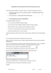
For the computation of the convective heat transfer one needs to know both the
temperature and the velocity of the gas close to the surface. Unfortunately, there is no
good model available that would give these quantities for a point downwind from a
burning area of arbitrary shape. Therefore, a series of CFD simulations was carried out
using the NIST Fire Dynamics Simulator software [McGrattan et al. 2002] where the
properties of leaning fire plume flowing over a building was studied in a twodimensional geometry. An example of the flow is shown in Figure 2 showing the
temperature field of a leaning fire plume. The building is on the left and the distance
14
from the building wall to the 5 m wide fire is 15 m. The wall height is 4 m. In the
simulations, the wall to fire distance L was varied from 5 to 20 m, heat release rate of
the fire Q& ¢¢ was varied from 50 to 1000 kW/m2 and windspeed Uw from 0 to 15 m/s. At
each combination, the maximum gas temperature in the vicinity of the wall and the
corresponding flow velocity were used for the calculation of the convective heat flux. A
first order (linear) polynomial was then fitted to the data using the least-squares
technique. As a result, we got the following formula that gives the convective heat flux
to a wall at ambient temperature (20 °C)
q& c¢¢ (U w , L, Q& ¢¢) = 282.9 + 0.8948Q& ¢¢ - 52.27 L + 166.1U w (W)
(9)
This formula is valid for the ranges mentioned above. During the application to the wall,
the convection flux must be corrected for the increased wall temperature. This is done
by decreasing the convective heat transfer by h (Twall - T0), assuming h = 5 W/mK.
Figure 2. An example of the FDS simulation of the interaction of a building (on the left)
and a wind driven fire plume with windspeed of 5 m/s, heat release rate of 1 MW/m2
and fire to wall distance of 15 m.
We assume that all the cells that are located within a 90 degrees wide sector upwind
from the building may contribute to the convective heat transfer. This 'upwind' area is
found by going to each cell inside the ignition neighbourhood (see Appendix A), and
calculating the angle between the wind direction and line from cell centre to building
centre. If the angle is less or equal to 45 degrees, the cell belongs to the 'upwind' area.
This technique is illustrated in Figure 3. The above correlation is then applied to each
cell inside the 'upwind' area, and the highest heat flux is chosen to for the heat transfer
calculation of all four walls of the building. This is somewhat inaccurate but
conservative approximation. To summarize, the radiative heat flux of the building wall
depends on the direction of the wall (north, east, south or west) but the gross convective
heat flux is the same for each wall.
15
'UPWIND' AREA
OF CONVECTION
BUILDING
WIND
DIRECTION
Figure 3. Defining the upwind area of convective heat transfer from forest fire to
building walls.
For the calculation of the wall heat transfer, the walls are assumed to be thermally thick,
and one-dimensional heat conduction equation for the material temperature is applied in
the direction x pointing into the solid (the point x = 0 represents the surface)
r w cw
¶Tw
¶T
¶ æ ¶T ö
= ç k w w ÷ ; - k w w (0, t ) = q& c¢¢ + q& ¢r¢
¶t
¶x è
¶x ø
¶x
(10)
where rw, cw and kw are the constant density, specific heat and conductivity of the
material; q& c¢¢ is the convective heat flux and q& ¢r¢ is the net radiative heat flux to the
surface. Similar boundary condition is applied to the back surface, assuming convection
and radiation to a space at ambient temperature. The above equation is solved using a
finite difference method with uniform grid in the x-direction and the same time step that
is used for the forest fire spread. An implicit Crank-Nicholson scheme is used for the
time integration. The temperature field of the wall is solved only to the point when the
surface reaches the ignition or breaking temperature given by the user.
2.6 Ignition of surface fires from explosion
During the explosions hot and burning fragments are ejected to the surroundings. These
fragments may ignite the forest fuels and cause a rapid spreading of the forest fire to a
large area. The formation mechanism of the fragments is an extremely complicated
process that depends on the mass and properties of the explosive material and its
container. In MASIFIRE, we do not attempt to predict the explosion behaviour of the
16
explosive objects, but let the user define all the necessary information. Starkenberg et
al. [2001] have studied the propagation probabilities of ammunition stacks, being able
to produce probability vs. distance curves for various propagation mechanisms, i.e.
detonation, burning, mechanical damage or mechanical hit. Here we assume that the
probability of ignition of the dead surface fuels behaves analogously and define a
probability curve using two distances R1 and R2: The probability of ignition is measured
as number of ignitions per area. At distances shorter than or equal to R1, the number of
ignitions is 1/m2. At R2 the number of ignitions is 0.1/m2 and zero outside the radius of
R2. Between these two values the ignition density varies proportional to 1/r2. The
definition of the ignition density curve is illustrated in Figure 4. The parameters R1 and
R2 are always associated with the storage building and are not affected by the contents
of the building.
Figure 4. Definition of the surface fire ignition curve.
17
3. System requirements and installing MASIFIRE
3.1 Hardware and software requirements
Both the speed of the computation and the memory requirement are strongly dependent
on the size of the map used in the simulation. For speed, the rule is simple: Faster CPU
is always better. A rough estimate of the memory requirement set by MASIFIRE is
Memory requirement = 22 * N * 8 / 1E6 [MBytes]
where N is the number of pixels in the map. In addition to this, Matlab itself typically
requires tens of megabytes of memory. For a map with 1000 ´ 500 pixels, the
MASIFIRE's memory requirement would therefore be approximately 88 MB. Similarly,
for a map with 2000 ´ 2000 cells, it would be 704 MB! It is easy to see, that the use of
maps with too high resolution or too wide area should be avoided. For graphics, a
monitor with a minimum of 1152 by 864 resolution and 16 bit colours is needed. A
1280 by 1024 resolution is recommended.
MASIFIRE is a Matlab GUI-application (GUI = graphical user interface) with
additional simulation routines (MEX-libraries) programmed with C-language. To run
MASIFIRE either of the following environments is needed:
·
Matlab 7.0 (R14) or higher.
·
Matlab Component Runtime (MCR) of release R14 or higher installed on the
computer. (This option is not valid until a precompiled version of MASIFIRE
becomes available.)
Binary versions (.dll) of the MASIFIRE MEX-libraries are available for Microsoft
Windows operating system. For other operating systems (e.g. Linux), users have to
compile the mex files by themselves. The following steps are required to compile:
mex
mex
mex
mex
runmasi.c fireLibmex.c
firelibgetfuel.c fireLibmex.c
mapimg.c
mapfix.c
18
3.2 Installing MASIFIRE
MASIFIRE is distributed as a Matlab GUI package that needs many files to work.
Below is a list files needed in MASIFIRE 1.0. Copy these files to an installation
directory, and add that directory to Matlab path.
M-files:
BuildingSetup.m
arrow.m
FuelCatalogManager.m showwindow.m
FuelSetup.m
findtoxicarea.m
windplume.m
mfsettings.m
GetNumberDialog.m
masifire.m
Fig-files:
BuildingSetup.fig
masifire.fig
GetNumberDialog.fig
FuelSetup.fig
FuelCatalogManager.fig
mfsettings.fig
MEX-files (dll-files on Windows systems)
fireLibGetFuel.dll
mapfix.dll
mapimg.dll
runmasi.dll
Alternatively, MASIFIRE can be distributed as an executable masifire.exe, compiled
with Matlab Compiler. To run masifire.exe, install first Matlab Component Runtime
(MCR) by running the MCRInstaller.exe.
IMPORTANT: Make sure that the directory path of Matlab
Component Runtime does not contain spaces. In general, any
Matlab components should not be installed under C:\Program
files -directory. Spaces in directory names may cause errors in
some Matlab functions.
19
4. User interface
4.1 Main window
When you start MASIFIRE, either by typing 'masifire' to a MATLAB prompt, or by
running the masifire.exe (MCR version), the main window opens on your screen. By
default, the window is maximized to full your screen, but you can make it smaller as usual.
Figure 5. MASIFIRE main window.
The main window contains the following areas:
4.1.1 Map axis
The map axis is used to visualize the map image and to show the proceeding of the fire
fronts and burning area. The burning and burn-out areas are shown by changing the
colour of the map. The colours depend on the original colour of the map. The colours
for white background colour are shown in Figure 6. You can zoom the map with mouse
by selecting the zoom-tool from the toolbar, or by pressing z-key.
20
Figure 6. The colours of the burning and burn-out surface fuel (left image) and canopy
fuel (right image) on a white background.
4.1.2 Fuel map tools
On the 'Fuel map tools' panel you can choose any of the available fuel models from the
scrollable list box, and either make it a default fuel, or bind that fuel to some of the map
colours. To bind or unbind a fuel model, click on the button with lock
or open lock
, respectively.
New colours can be added to the map by painting and outlining. In both operations,
mouse is used to define the area. In painting, the mouse pointer is used moved by left
mouse button down to add the colour. In outlining, the borders of the coloured area
should be given. After the painting, the colour should be bound with some of the fuel
models, but outlining always uses the fuel currently selected.
4.1.3 Object tools
The second panel on the left hand side is the 'Object tools' panel. There you can choose
some of the object types, add the objects on the map or delete existing objects. The
object types are
·
Ignition point. Add ignition points by clicking the left mouse button over the
map. Stop adding by clicking the right mouse button. The ignition points appear
21
on the map as red circles. When you add an ignition point, the ignition time of
the corresponding cell of the fuel map is set to the current time. Delete ignition
points one by one by selecting Ignition points from the menu, pressing 'Delete'
button and clicking the mouse over the point.
·
Ignition area. A larger area of the map can be set on fire in the beginning by
adding an ignition area. Add the corners of the area (as many as you wish) by
clicking the left mouse button. Right mouse button adds the last corner. Be sure
not to bring any other program window on the top of the MASIFIRE window
when adding ignition area. Delete and existing ignition area by selecting Ignition
area from the menu, pressing 'Delete' button and clicking the mouse over the
area.
·
Altitude contours. For the definition of the terrain you can add altitude contours
by clicking the points of the contour with left mouse button. Right button adds
the last point, after which you are asked to click the mouse inside the contour if
you are defining a hill, or outside if you are defining a pit. All the contours must
be closed and non-overlapping. If the contour continues outside the map you
should add at least two points outside the visible map area, as shown in Figure 7.
The accurate locations of the points outside the map are usually not very
important. When you have added all the contours, you should generate the
terrain (Tools-menu) and visually check it (Tools-menu /Show terrain). The map
should have the correct scaling before the adding of the contours because the
contours are not updated by any scaling operations. Delete an altitude contour by
selecting Altitude contour from the menu, pressing 'Delete' button and clicking
the mouse inside the contour.
·
Adding and deleting buildings. In the end of the object Pop-up menu are listed
the available building types. Add a building by pressing 'Add' button and
clicking your left mouse button over the map. Delete a building by pressing
'Delete' and clicking over an existing building. The available building types are
defined in the 'Building definitions' -tool (Settings menu).
22
Figure 7. Adding an altitude contour on the edge of the map.
4.1.4 Simulation tools
The third panel on the left hand side of the MASIFIRE main window is used for
running the simulations. Give the simulation time by typing it into the text box in
minutes, and run the simulation for the given amount of time by pressing the 'Run'
button. MASIFIRE will
Pressing 'Clear' will clear the results and set the time to zero. Select additional results by
selecting one of the following:
·
HRR. When selected, MASIFIRE plots the total heat release rate in a separate
window in the end of the simulation period.
·
Species. When selected, MASIFIRE plots the production rates of the current list
of species in a separate window in the end of the simulation period.
23
·
Evacuation. When selected, MASIFIRE plots the evacuation areas on the map,
and plots the maximum evacuation distance for each species in a separate
window. The evacuation areas are shown with colourful lines. One line
corresponds to one species and one concentration limit (8h or 15 min exposure).
The legend on the right hand side of the main window explains the colours. If
the legend goes under the map, deselect the 'Evacuation' and select again.
4.1.5 Wind
The last panel on the left hand side of the MASIFIRE main window is used for the
definition of wind speed (m/s) and direction. The wind speed should correspond to the
speed in the open flat terrain, at height of 6.1 m. The direction is defined as degrees
from north in clock-wise direction. Set the direction either by typing in the degrees as a
number or by dragging the red arrow with left mouse button. The left arrow becomes
visible when the map is read in.
4.2 Fuel setup window
The calculation of fire spread in forest and surface fuels is based on the definition of
fuel models and their association to the different areas of the map. Every type of
vegetation that appears on the map should have an own fuel model. MASIFIRE stores
the fuel models in fuel catalogs, which makes it easier to organize, save and load the
fuel models. The fuel catalogs and fuel models are defined on a Fuel setup window,
which starts from the Settings menu of the main window. Fuel setup window is shown
in Figure 8.
4.2.1 Fuel catalog
In the 'Fuel catalog' panel you can create new catalogs, save the selected catalog on the
hard disk, load a previously saved catalog and close the selected catalog. Pressing 'Fuel
catalog manager' button opens a separate dialog, where you can copy individual fuel
models from a catalog to another. This is very useful when you create new fuel models
by modifying existing models, and want to collect the new fuel models to a separate
catalog.
When MASIFIRE is started, the fuel catalog is initialized with 13 standard fuel models
[Anderson 1982].
24
Figure 8. Fuel setup window.
4.2.2 Fuel model
The individual fuel models of the currently selected fuel catalog are defined in the 'Fuel
model' panel. In the top of the panel is a Pop-up menu which is used to select the fuel
model. If the fuel model is modified, the changes should be saved by pressing the
'Apply' buttons. Buttons are also available for removing the fuel model from the catalog,
creating a new model, or copying the current fuel to the end of the catalog (Clone).
Fuel model's Name and Description are text strings, used to identify the model.
Wind reduction factor is used to calculate the actual wind speed at the ground fire flame
height (typically 1 to 2 m), by multiplying the open terrain wind speed given in the main
window. The default value is 0.3 but even values 0.1 may be used for dense fuels.
25
4.2.3 Surface fuel
In 'Surface fuel' panel you should give the following properties for the surface fuel:
·
Depth (m) is the height of the fuel layer from the ground.
·
Moisture content of dead fuel extinction (%) is the critical moisture of dead
fuels, above which they are not assumed to burn.
The natural fuels are not homogenous material but a wide distribution of different
grasses, shrubs, litter and live vegetation. To describe this kind of mixture of fuels with
a relatively small number of properties, strong simplifications must be made. To
describe the range of the different contents, each surface fuel may consist of up to four
(minimum one) classes of fuel types, called particles. Each particle class has the
following properties:
·
Particle type is either dead, live herbaceous, or live woody stem.
·
Load is the mass of particles per unit area (kg/m2).
·
The particle size is defined as surface area to volume ratio (AVR), which can be
calculated for spherical particles as AVR = 6/d and for cylindrical particles as
4/d. Here d is the particle diameter. AVR has units 1/m.
·
Density is the oven-dry density of the material (kg/m3).
·
Heat of combustion is the energy that is released when one unit mass of particle
mass burns (MJ/kg).
·
Total mineral content (%), effective mineral content (%). See Rothermel [1972]
for details.
·
Moisture content. Each particle type may be given own moisture content. These
values are used only if 'Fuel dependent moisture' is checked on the 'Moisture
scenario' panel of the Fuel setup window. (This feature is not implemented in
MASIFIRE 1.0).
26
4.2.4 Canopy fuel
In order to predict the initiation and spreading of crown fires, the properties of the
canopy should be defined for all fuel models. The 13 standard fuel models do not have
canopy at all. The definition of canopy fuel is simpler than the surface fuels, as there is
only one class of fuel particles. 'Canopy fuel' panel has the following fields:
·
Load is the available canopy fuel per unit area (kg/m2). This can be estimated
using the information on the canopy biomass of trees and the number of trees per
square meter.
·
Canopy height is approximately the height of the trees from the ground (m).
·
Canopy base height is the lowest height above the ground at which there is a
sufficient amount of canopy fuel to propagate fire vertically into the canopy.
·
Heat of combustion is the energy that is released when one unit mass of canopy
mass burns (MJ/kg).
·
Foliar moisture content is the moisture content of the fuel particles (%).
·
Area to volume ratio (1/m) is the measure of typical particle size. See the
explanation of the surface fuel properties.
4.2.5 Toxic species yields
This panel is used to define what is the yield of each toxic species for the current fuel
model. The yield is defined as a released mass per one kg of burned fuel. To modify the
yield values, choose the species from the list, type in the new value into the text box
below, and press enter.
4.2.6 Moisture scenario
The moisture of the fuel may be either fuel specific or global. Global settings are handy
when you want to study the effect of the weather or daytime on the whole simulation
area. (The fuel dependent moisture scenario is not implemented in MASIFIRE 1.0).
Five different moisture content values are used:
27
·
Wood means the moisture of the live woody fuels. The default is 150 %. Woody
fuels are perennial and usually have surface-area-to-volume ratios from 3300 to
6600 1/m.
·
1h, 10 h and 100 h mean the moisture contents of size categories of dead fuels
corresponding to one-hour, ten-hour and hundred-hour drying times. The onehour (1-h) timelag dead fuel category includes fuels from 0 to 0.64 cm in
diameter, the ten-hour (10-h) timelag dead fuel category includes fuels from
0.64 to 2.54 cm in diameter, and the hundred-hour (100-h) timelag fuel category
includes fuels from 2.54 to 7.62 cm in diameter. Larger fuels are not considered
in the simulation.
·
Herbaceous means the moisture of live herbaceous fuels. Live herbaceous fuels
usually have surface-area-to-volume ratios from 4900 to 11,500 1/m.
4.3 Building setup window
For the definition of building types, a separate Building Setup window is used. You can
enter Building Setup from the Settings menu of the MASIFIRE main window. Building
Setup window has three sections; the actual building types are defined in own panel on
the right. Possible contents of the building and wall types are also defined in own
panels. The basic rule is that before the ignition, the behaviour of the building is
determined by its wall type, as the walls are heated up by the forest fire. After the
ignition the contents of the building determine its behaviour.
In the up left corner of the window are buttons for saving and loading of the whole
setup on the hard disk. 'Load' button replaces the current settings by the contents of the
loaded file. 'Load Increm.' load the contents incrementally, adding the building, content
and wall types to the end of the corresponding lists of current types. Building Setup
window is shown in Figure 9.
4.3.1 Content Types
After the ignition, the behaviour of the building is determined by its contents. In this
panel you can modify or remove the existing content types, create new types or make a
clone of the current type. Press 'Apply' to save the modifications to the currently visible
content type. Each content type has the following fields:
28
Figure 9. Building Setup window.
·
Name and Description are used to identify the content type.
·
Type defines the hazard division, and is one of the following
o Combustible
- No explosion can take place
o Explosive 1.1 - Explosives with a mass explosion hazard
o Explosive 1.2 - Explosives with a projection hazard
o Explosive 1.3
- Explosives with predominantly a fire hazard
This information is currently used only to make a distinction between
combustible and explosive materials. How the material actually behaves,
must be defined by the user.
·
Ignition delay (s) is the time that is needed from the ignition or breaking of the
building walls to the ignition of the content. However, if some of the explosive
contents of the building ignites (explodes), all the other contents are also ignited.
Ignition delay and growth time parameters are explained in Figures 10 and 11
for combustible and explosive fuels, respectively.
29
·
HRRPUA, the heat release rate per unit area (kW/m2), is used to calculate the
heat release rate of combustible content.
·
Heat of combustion DHc (MJ/kg) is used to predict burning time of combustible
content.
·
Growth time (s) tg determines the time constant of the heat release rate
development. For combustible fuels it is the growth rate of the t2-type heat
release rate curve (the time when the heat release rate reaches 1000 kW). In fire
safety engineering, the growth times are usually defined based on the following
categories:
Growth type
Growth time tg (s)
Typical material
Slow
600
Floor coverings
Medium
300
Shop counters, office furniture
Fast
150
Bedding, displays and padded workstation partitioning
Ultra fast
75
Lightweight furnishing, upholstered
furniture, packing material in rubbish
pile, cardboard or plastic boxes in
vertical storage arrangement
< 75
Combustible liquids
For explosives, the growth time is the duration of the explosions. Ignition delay
and growth time parameters are explained in Figures 10 and 11 for combustible
and explosive fuels, respectively.
·
The yields of toxic species from the burning or explosion of the content is
defined in a way similar to the fuel model definition, in the previous section.
30
Figure 10. Definition of the heat release rate curve for combustible fuel.
4.3.2 Wall types
Each building has walls of some defined type. This panel allows the modification and
removing of existing wall types, definition of new wall types and cloning of the current
wall type to the end of the list. Press 'Apply' to save the modifications to the currently
visible wall type. Each wall has the following properties:
·
Name and Description are used to identify the wall type.
·
Thickness, conductivity, density and Specific heat are the physical and thermal
properties of the wall. These properties should include the effect of the moisture,
as the moisture content of the material is not separately defined.
·
Ignition temperature is the critical wall surface temperature where the wall is
assumed to ignite. This method can be applied to, for example, wooden walls.
·
Breaking temperature is the critical wall surface temperature where the wall is
assumed to break down. This method can be applied to wall that are made of, for
example, gypsum board.
31
Figure 11. Definition of the heat release rate curve for explosive fuel.
4.3.3 Building Types
This panel allows the modification and removing of existing building types, definition
of new types and copying (Clone) of the building type to the end of the list for further
modification. Press 'Apply' to save the modifications to the currently visible building
type. Each building has the following properties:
·
Name and Description are used to identify the building type.
·
To start the fire from the building, the checkbox with text 'Ignite in the
beginning' should be selected. The contents of the building will then ignite after
the ignition delays corresponding to each content type.
·
Wall type refers to one of the types defined in the 'Wall Types' panel. Each
building is assumed to have four walls (north, east, south and west) of same type.
·
Vent area (m2) is area of openings on each wall. (This property is here for future,
not used in MASIFIRE 1.0.)
·
To reduce the probability of fire spread from a forest fire to a building, the forest
fuel is typically cleared from the close neighbourhood of the building. Inside the
outer clearing distance there is some fuel, which is defined in the 'Fuel' Pop-up
menu. This is typically some surface fuel like grass. Inside the inner clearing
distance there is no fuel at all. This is typically from zero to few meters.
32
·
Each building may have up to four types of content. These types of contents are
selected from the four pop-up menus, and the mass (kg) and surface area (m2) of
the content are given below.
·
Both the combustible and explosive content may cause the ignition of the
surface fuels surrounding the building. The ignitions take place during the time
period set by the shortest ignition delay and heat release rate growth time of the
current contents. The probability of ignitions is defined as number of ignitions
per square meter of forest. The first radius corresponds to the ignition density of
1/m2 and the second for 0.001 ignitions /m2. See Figure 4 for more details.
4.4 General parameters
Some general parameters of MASIFIRE can be set using the 'General parameters'
window, which is entered from the Settings menu of the main window. A picture of the
window is shown in Figure 12. The available parameters are
·
Simulation time step (min). This is the initial and maximum value of the
simulation time step. During the simulation the time step is adjusted as
explained in Section 2.3.
·
Map pixel size (m). The scale of the map is determined by the size of the pixels
in meters. The scale can be modified either by typing the pixel size directly, or
by calibrating the map scale using some known distance on the map. See section
5.2.1.
·
Mapfix neighbourhood. This integer number determines the radius of the
neighbourhood during the MapFix operation. See Appendix A and Section 4.4.
·
Ignition point radius (m) is the size of the red circles showing the location of
ignition points on the map. The same length is also used as a size of the
buildings.
·
Printing interval (min) determines how often the proceeding of the simulation is
shown on the map.
·
Spread neighbourhood determines the number of cells in each direction for
which the ignition time is calculated during the fire spread modelling. Higher
number gives smoother spreading patterns, but may lead to unexpected
behaviour in some cases like narrow fire barriers (e.g. water streams).
33
·
Height difference between altitude contours (m) is used in the generation of
altitude terrain.
·
Resolution for the 3D terrain visualization (200) is the number of points in xdirection when the 3D surface of the terrain is generated.
·
'Show map objects in 3D image' should be selected if the objects like buildings
and ignition areas should be displayed in the 3D surface of the terrain.
·
The list of toxic species is defined here. The buttons on the right let the user
introduce new species, remove some of the current species and save the changes.
To modify the properties of a species, select it from the menu and type in the
emission factors and concentration limits to the corresponding text boxes. Use
NaN, if the information is not available. Remember to save the changes.
Figure 12. General parameters window.
34
4.5 Menus
4.5.1 File menu
The file menu contains the following items:
Open Workspace
Opens previously saved workspace. Workspace is a binary file
with extension .mat. The workspace files of the future MASIFIRE
versions are not necessarily backward compatible.
Save Workspace
Saves the current workspace to a binary file with extension .mat.
The workspace file contains all the necessary information for later
continuation of the work.
Save As Workspace
Saves the current workspace to a new file.
Read Map
Asks the file name of the map image and reads it using Matlab's
imread -function. The requirements for map images are explained
in Section 5.2.1.
Load terrain
Loads previously saved terrain information. Terrain files are
binary files with extension .ter. The loaded terrain must be
compatible with the current map.
Save terrain
Saves the current terrain and the altitude contours to a binary file.
Export time series
Writes the current time series data to a text file. The file contains
the following information: Time (s), heat release rate (kW), the x
and y-co-ordinates of the fire center point (m), fire area (m2),
emissions of the toxic species (kg/s) and evacuation distances
(km) corresponding to each species, if the evacuation was
selected from the Main window simulation tools.
Close
Exits MASIFIRE. Please note that the program always exits
without asking if the workspace should be saved.
35
4.5.2 Settings menu
Building setup
Opens the Building setup window (Section 4.3)
Fuel setup
Opens the Fuel setup window (Section 4.2)
General parameters Opens the General parameters window (Section 4.4)
Grid on
Toggles the visibility of grid on the map.
Show altitude contours Toggles the visibility of altitude contours on the map.
Highlight map altitudes with colour
Toggles the visualization of altitude information on the map. If
selected, high areas are shown as red in the map.
Show building names Toggles the visibility of building type next to each building object
on the map.
Show building wall temperatures
Toggles the visibility of the building wall surface temperature
inside each building object on the map. Maximum of the four
walls (north, east, south, west) is shown.
Save images
Toggles the saving of the map images during the simulation. If
selected, MASIFIRE will save an image of the map, including the
fire spread patterns, at every print interval. The jpg-images are
saved into a runmasi directory under the current working
directory.
Figure menu
Toggles the visibility of Matlab's Figure window menus. These
menus contain many useful tools for the controlling of figures.
4.5.3 Tools menu
Calibrate map scale
This tool allows the calibration map pixel size (i.e. scale) by
letting the user click two points from the map, and then asking for
the distance between the points in meters. This is useful, if the
map contains some landmarks with known distance.
36
Resample map image This tool allows the resampling of the map image in order to
increase or decrease the resolution. The tool asks for a new pixel
size in meters, and then calculates new map image. After the
operation the size of the map has changed in terms of pixels, but
the distances are the same. The new pixel size is usually not
exactly the one that was asked, but as close to that as possible.
Due to the strong dependence of the simulation speed and
memory requirements on the size of the map image. It is often
useful to decrease the resolution.
Reduce map colors
This tool can be used to reduce the number of colours on the map.
A set of new colours is determined from the original colour
palette by the reduction factor given by the user and then all the
colours are mapped to the closest colour of the new palette. The
user can accept or reject the result. Different values of the
reduction factor should be tested. The tool should be used before
any simulations have been made.
Add altitude contour
Asks user to click the points for a new altitude contour. Same
operation as pressing 'Add' button on the 'Object tools' panel
when Altitude contour is selected from the menu.
Generate terrain
Calculates the altitude terrain, i.e. the altitude of each map pixel,
by interpolating from the altitude contours. Cubical interpolation
is used.
Show terrain
Visualization of the altitude terrain as three-dimensional surface.
The altitudes are multiplied by a factor of five to improve the
visualization.
37
5. Operational instructions
5.1 Steps of a typical simulation process
The steps of a typical simulation process are listed below.
1.
Have the map image available as a file on your hard disk. See Section 5.2.1 for
requirements on the image. It is best to make a separate folder for your
simulation.
2.
Start Matlab, change to the directory where you have the map, and start
MASIFIRE by typing masifire to the Matlab prompt (This assumes you
have the MASIFIRE installation directory in the Matlab toolbox path.)
Alternatively, start masifire.exe (not available for MASIFIRE 1.0).
3.
Read in the map. See Sections 4.5 and 5.2.
4.
If necessary, reduce the map colours using the tool available in Tools menu.
5.
Set the map scale (Section 5.2.2). It is important to scale the map before any
other operations below.
6.
Define the altitude terrain by first adding the altitude contours (Section 4.1.3)
and then generating the terrain (Section 4.5.3). Check the terrain visually.
7.
Set the list of toxic species on the General parameters window (Section 4.4).
The species list should always be defined before the definition of fuel and
building types because the changing of the species list initializes the emission
factors of fuel models and building content types.
8.
Define fuels models. You may use the standard fuels that are available when
the program starts, define some of your own or load an existing fuel catalog.
(Section 4.2).
9.
Bind fuel models to the existing map colours. If one vegetation type is
dominant in the simulation area, the corresponding fuel model should be made
the default fuel. Or if most of the map area is non-combustible, make 'No fuel'
the default. See Section 4.1.2 for more information on binding.
38
10. Bind the map colours that are used for map symbols, altitude contours and texts
to the text type appearing in the list of fuel models. If some of the map line
types consist of two or more colours, it is best to bind the outmost colour first.
Experiment with different MapFix neighbourhoods if the fire spread patterns
are not what you expected (Section 4.4).
11. Define new areas on the map using the Outline tool, Section 4.1.2. It is
important to bind the text types before the use of the outline tool.
12. Define building types. First define the wall and content types, then the actual
building types (Section 4.3). If the definitions are available in an existing
database, load the database. It is important to have the forest fuel types defined
before the building definition.
13. Add building on the map (Section 4.1.3).
14. Add ignition source. It may be either one or more ignition point, ignition area
or a building serving as ignition source (Sections 4.1.3 and 4.3).
15. Set wind speed and direction (Section 4.1.5).
16. Select the desired additional output: HRR curve, Species emissions or
evacuation distances (Section 4.1.4).
17. Set the simulation time in minutes and run the simulation (Section 4.1.4).
18. Repeat the steps 14 to 17 as long as needed. However, you may not add other
ignition source than ignition points.
19. Export time series, if needed (Section 4.5.1).
20. Save the workspace for later use (Section 4.5.1).
21. Close MASIFIRE (Section 4.5.1).
39
5.2 Using maps
5.2.1 Map image
Map image is the basis for the whole simulation. The method how the image is obtained
is not important, but the quality of the map image is important. Therefore, scanned
images should be used with care. The following properties are important for the image:
·
The image file should contain three colour components for each pixel (R,G,B).
·
The image should contain as few colours as practical to enable the easy but
sufficient identification of the vegetation types. If the map colours are
continuous or shading, decrease the colour depth using some image processing
software. Do not use image formats with lossy compression (typically JPEG)
because the lossy compression will alter the colours slightly. Colour reduction
tool is available in the Tools menu, Section 4.5.3.
·
The resolution should be sufficient so that all the important details can be found,
but not too high to keep the simulation times and memory requirements
reasonable. The map should not cover too large area. Use image processing
software to include only the area of importance. The map resolution can be
changed in MASIFIRE using the 'Resample map image' tool available in the
Tools menu, Section 4.5.3.
The supported file types are
JPEG
8-bit and 12-bit lossless compressed RGB images
TIFF
24-bit uncompressed images; 24-bit images with packbits compression; and
48-bit RGB images
BMP
24-bit, and 32-bit uncompressed images
PNG
24-bit and 48-bit RGB images.
5.2.2 Setting map scale
Digitized maps consist of pixels, and each pixel has therefore some finite area that it
covers. In MASIFIRE, each pixel is used as a cell for the spreading algorithm. It is
therefore extremely important that the size of the pixel is correctly set. There are two
ways of doing this:
40
1. User may enter the pixel size in meters to the General parameters window
(Section 4.4). This is useful when the map comes from some commercial
computer map library, where the pixel size can be found.
2. User may calibrate the map by choosing the calibration tool (Section 4.5.3).
User is asked to click on two points on the map, and then type the distance
between the points in meters.
5.3 Defining fuels
5.3.1 Choosing one of the standard fuels
The following instructions are taken from BEHAVE 2.0. They give a step-by-step
procedure how to choose the best surface fuel model of the 13 standard models. The
standard models and their properties are listed in Table 2.
Table 2. The standard surface fuel models [Anderson 1982]. Mo.Ext. is the moisture
concentration where the fuel does not burn anymore.
Fuel loading (kg/m 2)
Surface-area-to-volume-ratio (1/m)
Fuel no
1h
10 h
100 h
Live
1h
1
0.17
0
0
0
11483
2
0.45
0.22
0.11
0.11
9842
3
0.67
0
0
0
4921
4
1.12
0.90
0.45
1.12
6562
358
5
0.22
0.11
0
0.45
6562
358
6
0.34
0.56
0.45
0
5741
358
98
7
0.25
0.42
0.34
0.08
5741
358
98
8
0.34
0.22
0.56
0
6562
358
98
30
9
0.65
0.09
0.03
0
8202
358
98
25
10
0.67
0.45
1.12
0.45
6562
358
98
11
0.34
1.01
1.24
0
4921
358
98
15
12
0.90
3.15
3.71
0
4921
358
98
20
13
1.57
5.16
6.29
0
4921
358
98
25
1h
=
0... 0.64 cm
10 h
=
0.64 ... 2.54 cm
100 h
=
2.57 ... 7.62 cm
41
10 h
100 h
Live
Mo.Ext (%)
12
358
98
4921
15
25
98
4921
20
4921
20
25
5085
4921
40
25
Observations
1. Determine the general vegetation type, i.e., grass, brush, timber litter, or slash.
2. Estimate which stratum of surface fuel is most likely to carry the spreading fire.
For instance, the fire may be in a timbered area, but the timber is relatively open
and the dead grass, not needle litter, would carry the fire. In this case, fuel model
2, which is not listed as a timber model, should be considered. In the same area
if the grass is sparse and there is no wind or slope, the needle litter would be the
stratum carrying the fire and fuel model 9 would be a better choice.
3. Note the general depth and compactness of the fuel. This information will be
needed when using the fuel model key. These are very important considerations,
particularly in the grass and timber types.
4. Determine which fuel classes are present and estimate their influence on fire
behaviour. For instance, green fuel may be present, but will it play a significant
role in fire behaviour? Large fuels may be present, but are they sound or
decaying and breaking up? Do they have limbs and twigs attached or are they
bare cylinders? You must look for fine fuels and choose a model that represents
their depth, compactness, and to some extent, the amount of live fuel and its
contribution to fire. Do not be restricted by the fuel model name or category.
Using these observations, proceed through the fuel model key and the descriptions
provided by Anderson (1982) to select a model.
Key to the Standard Fire Behaviour Fuel Models
I. PRIMARY CARRIER OF THE FIRE IS GRASS
Expected rate of spread is moderate to high, with low to moderate intensity (flame length).
A. Grass is fine structured, generally below knee level, and cured or primarily dead.
Grass is essentially continuous. Consider fuel model 1.
B. Grass is coarse structured. above knee level (averaging about 3 feet), and is
difficult to walk through. Consider fuel model 3.
C. Grass is usually under an open timber or brush overstory. Litter from the
overstory is involved, but grass carries the fire. Expected spread rate is slower
than fuel model 1 and intensity is less than fuel model 3. Consider fuel model 2.
42
II. PRIMARY CARRIER OF THE FIRE IS BRUSH OR LITTER BENEATH BRUSH
Expected rate of spread and fireline intensity (flame length) is moderate to high.
A. Vegetative type is southern rough or low pocosin. Brush is generally 2 to 4 feet
high. Consider fuel model 7.
B. Live fuels are absent or sparse. Brush height averages 2 to 4 feet. Brush requires
moderate winds to carry the fire. Consider fuel model 6.
C. Live fuel moisture can have a significant effect on fire behaviour.
1. Brush is about 2 feet high with light loading of brush litter underneath. Litter
may carry the fire, especially at low wind speed. Consider fuel model 5.
2. Brush is head high (6 feet) with a heavy loading of dead woody fuel. Very
intense fire with high spread rates are expected. Consider fuel model 4.
3. Vegetative type is high pocosin. Consider fuel model 4.
III. PRIMARY CARRIER OF THE FIRE IS LITTER BENEATH A TIMBER STAND.
Spread rate is low to moderate; fireline intensity (flame length) may be low to high.
A. Surface fuels are mostly foliage litter. Large fuels are scattered and lie on the
foliage litter; i.e., large fuels are not supported above the litter by their branches.
Green fuels are scattered enough to be insignificant to fire behaviour.
1. Dead foliage is tightly compacted, short needle (2 inches or less) conifer
litter or hardwood litter. Consider fuel model 8.
2. Dead foliage litter is loosely compacted long needle pine or hardwoods.
Consider fuel model 9.
B. There is a significant amount of larger fuel. Larger fuel has attached branches
and twigs, or has rotted enough that it is splintered and broken. The larger fuels
are fairly well distributed over the area. Some green fuel may be present. The
overall depth of the fuel is probably below the knees, but some fuel may be
higher. Consider fuel model 10.
43
IV. PRIMARY CARRIER OF THE FIRE IS LOGGING SLASH.
Spread rate is low to high; fireline intensity (flame length) is low to very high.
A. Slash is aged and overgrown.
1. Slash is from hardwood trees. Leaves have fallen and cured. Considerable
vegetation (tall weeds) has grown in amid the slash and has cured or dried
out. Consider fuel model 6.
2. Slash is from conifers. Needles have fallen and considerable vegetation (tall
weeds and some shrubs) has overgrown the slash. Consider fuel model 10.
B. Slash is fresh (0-3 years or so) and not overly compacted.
1. Slash is not continuous. Needle litter or small amounts of grass or shrubs
must be present to help carry the fire, but the primary carrier is still slash.
Live fuels are absent or do not play a significant role in fire behaviour. The
slash depth is about 1 foot. Consider fuel model 11.
2. Slash generally covers the ground (heavier loadings than fuel model 11),
though there may be some bare spots or areas of light coverage. Average
slash depth is about 2 feet. Slash is not excessively compacted.
Approximately one-half of the needles may still be on the branches but are
not red. Live fuels are absent, or are not expected to affect fire behaviour.
Consider fuel model 12.
3. Slash is continuous or nearly so (heavier loadings than fuel model 12). Slash
is not excessively compacted and has an average depth of 3 feet.
Approximately one-half of the needles are still on the branches and are red,
OR all the needles are on the branches but they are green. Live fuels are not
expected to influence fire behaviour. Consider fuel model 13.
4. Same as previous, EXCEPT all the needles are attached and are red.
Consider fuel model 4.
44
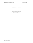
5.3.2 Determining the forest biomass
Surface fuels consists of bushes and small trees, understorey vegetation (dwarf shrubs
such as lingonberry and bilberry, grasses, mosses and lichen) and litter. A study of the
organic matter content of an old spruce forest in Northern Finland determined surface
fuel biomass to 1.05 kg/m2 [Havas & Kubin 1983]. About 30 % (0.15 kg/m2) of the
litter in the old spruce forest was larger than 6 mm in size and about 70 % (0.34 kg/m2)
smaller than 6 mm. Figure 13 gives the variation in understorey vegetation biomass in
coniferous forests with age of stand.
Canopy fuel consists of foliage and branches. The canopy biomass in an old spruce
forest was determined to 2.80 kg/m2 [Havas & Kubin 1983]. A tree-dependent estimate
is obtained by counting the number of trees per unit area and estimating an average
diameter at breast height for the trees. Figure 14 gives an average foliage + branch
biomass for one tree. The mass of canopy fuel per unit area can be calculated by
multiplying the average biomass of one tree with the number of trees per unit area.
0,8
Biomass (kg/m2)
0,6
0,4
0,2
Figure 13. Total biomass of understorey vegetation in coniferous forests (Muukkonen &
Mäkipää 2003).
45
175
Spruce, branch
Biomass/tree (kg)
150
Spruce, foliage
125
Spruce, total
100
Havas & Kubin
1983
75
50
25
0
0
10
20
dbh (cm)
30
40
125
Pine, branch
Pine, foliage
Biomass/tree (kg)
100
Pine, total
75
50
25
0
0
10
20
30
40
dbh (cm)
Figure 14. Generalised foliage and branch biomass curves for boreal spruce and pine
(Muukkonen 2004). Total = foliage + branch, dbh is diameter at breast height. Estimate
for average canopy biomass/tree in an old spruce forest in Northern Finland (Havas &
Kubin 1983) is added for spruce.
46
5.3.3 Creating new fuel models
If none of the standard fuel models appropriately describes the surface fuel, or the
crown fires should be included in the simulation, a new model should be created. The
easiest way of doing this is by copying the standard fuels to a new fuel catalog, and
modifying them. When you have modified any of the fuel model properties, remember
to press the 'Apply' button of the Fuel Setup window. Otherwise the changes are not
retained when you exit the Fuel Setup. When you have created a new catalog with
custom fuel models, you should save the whole catalog on the disk for later use.
47
6. Summary
Software for Map based Simulation of Fires in Forest-Urban Environment (MASIFIRE)
is described. The software can be used for the simulation of fire spread in forests with
surface and canopy vegetation, and the spreading of fire from the forest to buildings.
The model includes the effects of fuel type, wind, moisture and the shape of the terrain.
Model results include the fire spread, total heat release rate, production of toxic species
and necessary evacuation area for people. The fire spread algorithm is based on the
BEHAVE model developed by the U.S. Department of Agriculture, Forest Service. The
features of the user interface and the basic procedure of the use are also described.
48
Acknowledgements
The contributions of the following people are greatly acknowledged: Mr. Henri Biström
of VTT developed and implemented the treatment of altitude information. Dr. Tuomas
Paloposki and Dr. Esko Mikkola also of VTT provided important background
information, especially on the emission factors and concentration limits of toxic species.
Dr. Patricia Andrews of USDA Forest Service helped with the details of BEHAVE
model.
49
References
Andrews, P.L. 1986. BEHAVE: Fire Behaviour Prediction and Fuel Modeling System-BURN Subsystem Part 1. General Technical Report INT-194. Ogden, UT: U.S.
Department of Agriculture, Forest Service, Intermountain Research Station. 130 p.
Anderson, H.E. 1982. Aids to determining fuel models for estimating fire behavior.
General Technical Report INT-122. Ogden, UT: U.S. Department of Agriculture, Forest
Service, Intermountain Forest and Range Experiment Station. 22 p.
Battye, W. & Battye, R. 2002. Development of Emissions Inventory Methods for
Wildland Fire, Final Report. EPA Contract No. 68-D-98-046. Research Triangle Park,
NC: US Environmental Protection Agency. 82 p.
Bevins, C.D. 1996. fireLib User Manual and Technical Reference. Systems for
Environmental Management. 47 p.
Cohen, J.D. & Butler, B.W. 1998. Modeling Potential Structure Ignitions from Flame
Radiation Exposure with Implications for Wildland/Urban Interface Fire Management.
IAWF. 13th Fire and Forest Meteorology Conference. Lorne, Australia 1996. Pp. 81–86.
Finney, M.A. 1998. FARSITE: Fire Area Simulator-Model Development and
Evaluation. Res. Pap. RMRS-RP-4, Odgen, UT: U.S. Department of Agriculture, Forest
Service, Rocky Mountain Research Station. 47 p.
Havas, P. & Kubin, E. 1983. Structure, growth and organic matter content in the
vegetation cover of an old spruce forest in Northern Finland. Annales Botanici Fennici
Vol. 20, pp. 115–149.
HTP-arvot 2002. (Occupational exposure limits). Ministry of Social Affairs and Health.
Tampere. 55 p. (In Finnish).
McGrattan, K.B., Baum, H.R., Rehm, R.G., Forney, G.P., Floyd, J.E., Hostikka, S. &
Prasad. K. 2002. Fire Dynamics Simulator (Version 3) – Technical Reference Guide.
Technical Report NISTIR 6783, 2002 Edition, National Institute of Standards and
Technology, Gaithersburg, Maryland.
Memarzadeh, F. 1995. A Functional Explanation of a Point Source Gaussian Plume
Dispersion Model. 1995 ASME Cogen-Turbo Power Conference, August 23–24, 1995,
Vienna, Austria. 11 p.
50
Morvan, D. & Dupuy, J.L. 2004. Modeling the propagation of a wildfire through a
Mediterranean shrub using a multiphase formulation. Combustion and Flame 138
(2004), pp. 199–210.
Muukkonen, P. 2004. Generalised allometric volume and biomass functions for some
European tree species Cost e21 meeting "Task Force Meeting on biomass expansion
factors (BEFs) and allometric biomass equations". Hauho 16–19.5.2004. 11 slides.
Muukkonen. P. & Mäkipää, R. 2003. Biomass models of understorey vegetation
according to stand age and site quality in boreal coniferous forests. 15 slides.
Netterville, D.D.J. 1990. Plume Rise, Entrainment and Dispersion in Turbulent Winds.
Atmospheric Environment, Vol. 24A, No. 5, pp. 1061–1081.
Pastor, E., Zárate, L., Planas, E. & Arnaldos, J. 2003. Mathematical models and calculation
systems for the study of wildland fire behaviour. Progress in Energy and Combustion
Science, Vol. 29, pp. 139–153.
Persson, B. & Simonson, M. 1998. Fire Emissions into the Atmosphere. Fire
Technology, Vol. 34, No. 3, pp. 266–279.
Rehm, R., McGrattan, K.B. & Baum, H.R. 2002. Large eddy simulation of flow over a
wooded building complex. Wind & Structures, Vol. 5, No. 2–4(2002), pp. 291–300.
Rehm, R., Evans, D., Mell, W., Hostikka, S., McGrattan, K., Forney, G., Bouldin, C. &
Baker, E. 2003. Neighbourhood-scale fire spread. 5th Symposium on Fire and Forest
Meteorology, Orlando, FL, 16–20 Nov. 2003. The American Meteorological Society.
Rothermel, R.C. 1972. A mathematical model for predicting fire spread in wildland
fuels. Res. Pap. INT-115. Ogden, UT; U.S. Department of Agriculture, Forest Service,
Intermountain Forest and Range Experiment Station. 40 p.
Sandberg, D.V., Ottmar, R.D., Peterson, J.L. & Core, J. 2002. Wildland fire on
ecosystems: effects of fire on air. Gen. Tech. Rep. RMRS-GTR-42-vol. 5. Ogden, UT:
U.S. Department of Agriculture, Forest Service, Rocky Mountain Research Station. 79 p.
Scott, J.H. & Reinhardt, E.D. 2001. Assessing crown fire potential by linking models of
surface and crown fire behaviour. Research Paper RMRS-RP-29. Fort Collins, CO: U.S.
Department of Agriculture, Forest Service, Rocky Mountain Research Station. 59 p.
51
Starkenberg, J., Sullivan, J.D., Hillstrom, W.W., Lottero, R.E., Chin, W.K. & Mulkern, T.J.
2001. A Summary of Analysis and Test Support for the Munitions Survivability
Technology Program. ARL-TR-2506. Army Research Laboratory, MD. 42 p.
Tewarson, A. 2002. Generation of heat and chemical compounds in fires. In: DiNenno, P.J.,
Drysdale, D., Beyler, C.L. & Walton, W.D. (Eds.). SFPE Handbook of Fire Protection
Engineering, 3rd edition. Pp. 3-85–3-161.
52
Appendix A: Glossary
This glossary is mainly based on the glossary of Scott & Reinhardt [2001].
Active crown fire — A continuous crown fire in which the entire fuel complex
becomes involved and the fire spreads in the canopy fuels.
Available canopy fuel — The mass of canopy fuel per unit area consumed in a
crownfire. There is no post-frontal combustion in canopy fuels, so only fine canopy
fuels are consumed. We assume that only the foliage and a small fraction of the
branchwood is available.
Canopy base height — The lowest height above the ground at which there is a
sufficient amount of canopy fuel to propagate fire vertically into the canopy. Canopy
base height is an effective value that incorporates ladder fuels such as shrubs and
understory trees.
Canopy bulk density — The mass of available canopy fuel per unit canopy volume. It
is a bulk property of a stand, not an individual tree.
Canopy fuels — The live and dead foliage, live and dead branches, and lichen of trees
and tall shrubs that lie above the surface fuels. See also available canopy fuel.
Continuous crown fire — See active crown fire.
Crown fire — Any fire that burns in canopy fuels.
Fireline intensity — The rate of heat release in the flaming front per unit length of fire front.
Flaming front — The zone at a fire’s edge where solid flame is maintained.
Foliar moisture content — Moisture content (dry weight basis) of live foliage,
expressed as a percent.
Foliar moisture effect — A theoretical effect of foliar moisture content on active
crown fire spread rate.
Fuel model — A set of surface fuel bed characteristics (load and surface-area-tovolume-ratio by size class, heat content, and depth) organized for input to a fire model.
Standard fuel models (Anderson 1982) have been stylized to represent specific fuel
conditions.
A1
Ground fire — A slow-burning, smouldering fire in ground fuels. Contrast with
surface fire. Ground fuels— Fuels that lie beneath surface fuels, such as organic soils,
duff, decomposing litter, buried logs, roots, and the below-surface portion of stumps.
Compare with surface fuels.
Ignition neighbourhood — A rectangular area of the map around a building where the
forest fire may contribute to the heating of the building walls. Width and height of the
area are 2 ´ IgnitionRadius (100 m at the moment).
MapFix operation — An operation where MASIFIRE tries to determine the actual fuel
type of the cells that are marked as 'Text' type. For each 'Text' type cell, the most
common fuel type inside the MapFix neighbourhood is applied.
Passive crown fire — A crown fire in which individual or small groups of trees torch
out, but solid flaming in the canopy cannot be maintained except for short periods.
Passive crown fire encompasses a wide range of crown fire behaviour from the
occasional torching of an isolated tree to a nearly active crown fire. Also called torching
and candling. See also intermittent crown fire.
Plume-dominated fire — A fire for which the power of the fire exceeds the power of
the wind, leading to a tall convection column and atypical spread patterns. The fire
spread models used in MASIFIRE do not address plume-dominated fire behaviour.
Contrast with wind-driven fire.
Reaction intensity — The heat release rate of fire per unit area.
Surface fire — A fire spreading through surface fuels.
Surface fuels — Needles, leaves, grass, forbs, dead and down branches and boles,
stumps, shrubs, and short trees.
Total fuel load — The mass of fuel per unit area that could possibly be consumed in a
hypothetical fire of the highest intensity in the driest fuels.
Wind reduction factor — The ratio of the midflame windspeed to the open (6.1-m)
windspeed. For convenience of measurement eye-level winds are usually substituted for
midflame winds.
A2
VTT WORKING PAPERS
VTT RAKENNUS- JA YHDYSKUNTATEKNIIKKA –
VTT BYGG OCH TRANSPORT –VTT BUILDING AND TRANSPORT
4
Hietaniemi, Jukka, Hostikka, Simo & Vaari, Jukka. FDS simulation of fire spread - comparison of model
results with experimental data. 2004. 46 p. + app. 6 p.
6
Viitanen, Hannu. Betonin ja siihen liittyvien materiaalien homehtumisen kriittiset olosuhteet - betonin
homeenkesto. 2004. 25 s.
7
Gerlander, Riitta & Koivu, Tapio. Asiantuntijapalvelu yritysten innovaatiojohtamisen kehittämiseksi
Piilaakson osaamiseen tukeutuen. IMIT SV -hankkeen loppuraportti. 2004. 25 s. + liitt. 11 s.
11
Lakka, Antti. Rakennustyömaan tuottavuus. 2004. 26 s. + liitt. 15 s.
14
Koivu, Tapio, Tukiainen, Sampo, Nummelin, Johanna, Atkin, Brian & Tainio, Risto. Institutional complexity
affecting the outcomes of global projects. 2004. 59 p. + app. 2 p.
15
Rönty, Vesa, Keski-Rahkonen, Olavi & Hassinen, Jukka-Pekka. Reliability of sprinkler systems. Exploration
and analysis of data from nuclear and non-nuclear installations. 2004. 89 p. + app. 9 p.
18
Nyyssönen, Teemu, Rajakko, Jaana & Keski-Rahkonen, Olavi. On the reliability of fire detection and alarm
systems. Exploration and analysis of data from nuclear and non-nuclear installations. 2005. 62 p. + app. 6 p.
20
Simo Hostikka & Johan Mangs. MASIFIRE – Map Based Simulation of Fires in Forest-Urban Interface.
Reference and user's guide for version 1.0. 2005. 52 p. + app. 2 p.
ISBN 951–38–6571–1 (URL: http://www.vtt.fi/inf/pdf/)
ISSN 1459–7683 (URL: http://www.vtt.fi/inf/pdf/)