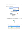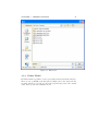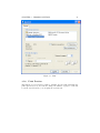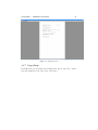
1
Gsi
User’s Manual
CMLP
SRR
2012
Contents
1 Introduction
6
2 Installing the program
2.1 Installation steps of the interface . . . . . . . . . . . . . . . . . .
2.2 Steps to incorporate the transportation program to the interface
8
8
15
3 Program Options
3.1 Models . . . . . . . . . . . . . . . . .
3.1.1 Add Model . . . . . . . . . .
3.1.2 Choose Model . . . . . . . . .
3.1.3 Edit Model . . . . . . . . . .
3.1.4 Delete Model . . . . . . . . .
3.1.5 Print . . . . . . . . . . . . . .
3.1.6 Print Preview . . . . . . . . .
3.1.7 Page Setup . . . . . . . . . .
3.1.8 Exit . . . . . . . . . . . . . .
3.2 Configuration . . . . . . . . . . . . .
3.2.1 Programs . . . . . . . . . . .
3.2.2 Number of Images . . . . . .
3.3 Edit . . . . . . . . . . . . . . . . . .
3.3.1 Find . . . . . . . . . . . . . .
3.3.2 Find Next . . . . . . . . . . .
3.3.3 Find Error . . . . . . . . . .
3.3.4 Font . . . . . . . . . . . . . .
3.4 Aggregations . . . . . . . . . . . . .
3.4.1 New Simple Aggregation . . .
3.4.2 New Composite Aggregation
3.4.3 Edit Aggregations . . . . . .
3.4.4 Delete Aggregations . . . . .
3.5 Simulations . . . . . . . . . . . . . .
3.5.1 New Simulation . . . . . . . .
3.5.2 Edit Simulations . . . . . . .
3.5.3 Delete Simulations . . . . . .
3.6 Results . . . . . . . . . . . . . . . . .
19
19
19
20
20
21
22
23
24
25
26
26
26
27
27
27
28
28
28
29
30
30
32
33
33
35
37
37
1
.
.
.
.
.
.
.
.
.
.
.
.
.
.
.
.
.
.
.
.
.
.
.
.
.
.
.
.
.
.
.
.
.
.
.
.
.
.
.
.
.
.
.
.
.
.
.
.
.
.
.
.
.
.
.
.
.
.
.
.
.
.
.
.
.
.
.
.
.
.
.
.
.
.
.
.
.
.
.
.
.
.
.
.
.
.
.
.
.
.
.
.
.
.
.
.
.
.
.
.
.
.
.
.
.
.
.
.
.
.
.
.
.
.
.
.
.
.
.
.
.
.
.
.
.
.
.
.
.
.
.
.
.
.
.
.
.
.
.
.
.
.
.
.
.
.
.
.
.
.
.
.
.
.
.
.
.
.
.
.
.
.
.
.
.
.
.
.
.
.
.
.
.
.
.
.
.
.
.
.
.
.
.
.
.
.
.
.
.
.
.
.
.
.
.
.
.
.
.
.
.
.
.
.
.
.
.
.
.
.
.
.
.
.
.
.
.
.
.
.
.
.
.
.
.
.
.
.
.
.
.
.
.
.
.
.
.
.
.
.
.
.
.
.
.
.
.
.
.
.
.
.
.
.
.
.
.
.
.
.
.
.
.
.
.
.
.
.
.
.
.
.
.
.
.
.
.
.
.
.
.
.
.
.
.
.
.
.
.
.
.
.
.
.
.
.
.
.
.
.
.
.
.
.
.
.
.
.
.
.
.
.
.
.
.
.
.
.
.
.
.
.
.
.
.
.
.
.
.
.
.
.
.
.
.
.
.
.
.
.
.
.
.
.
.
.
.
.
.
.
.
.
.
.
.
.
.
.
.
.
.
.
.
.
.
.
.
.
.
.
.
.
.
.
.
.
.
.
.
.
.
.
.
.
.
.
.
.
.
.
.
.
.
.
.
.
.
.
.
.
.
.
.
.
.
.
.
.
.
.
.
.
.
.
.
.
.
.
.
.
.
.
.
.
.
.
.
.
.
.
.
.
CONTENTS
3.6.1
3.6.2
3.7
3.8
Text . . . . . . . . . . . . . . . . . . . . . .
GDX-Charts . . . . . . . . . . . . . . . . .
3.6.2.1 Show L Values Only
43
3.6.2.2 Filter Data
44
3.6.2.3 Transform Table
47
3.6.2.4 Swap Indices
51
3.6.2.5 Configure chart
53
3.6.2.6 Precision
57
3.6.2.7 Save Template and Update Charts
58
3.6.3 Listings . . . . . . . . . . . . . . . . . . . .
3.6.3.1 Edit Listing . . . . . . . . . . . .
3.6.3.2 Delete Listings . . . . . . . . . . .
3.6.4 Excel . . . . . . . . . . . . . . . . . . . . .
3.6.4.1 Within Gsi . . . . . . . . . . . . .
3.6.4.2 Open with Excel . . . . . . . . . .
Window . . . . . . . . . . . . . . . . . . . . . . . .
3.7.1 Horizontal . . . . . . . . . . . . . . . . . . .
3.7.2 Vertical . . . . . . . . . . . . . . . . . . . .
3.7.3 Cacade . . . . . . . . . . . . . . . . . . . .
Help . . . . . . . . . . . . . . . . . . . . . . . . . .
3.8.1 Introduction . . . . . . . . . . . . . . . . .
3.8.2 Gsi Manual . . . . . . . . . . . . . . . . . .
3.8.3 Model . . . . . . . . . . . . . . . . . . . . .
3.8.4 About . . . . . . . . . . . . . . . . . . . . .
2
. . . . . . . .
. . . . . . . .
37
38
.
.
.
.
.
.
.
.
.
.
.
.
.
.
.
58
58
60
61
61
61
62
63
63
64
64
65
65
65
65
.
.
.
.
.
.
.
.
.
.
.
.
.
.
.
.
.
.
.
.
.
.
.
.
.
.
.
.
.
.
.
.
.
.
.
.
.
.
.
.
.
.
.
.
.
.
.
.
.
.
.
.
.
.
.
.
.
.
.
.
.
.
.
.
.
.
.
.
.
.
.
.
.
.
.
.
.
.
.
.
.
.
.
.
.
.
.
.
.
.
.
.
.
.
.
.
.
.
.
.
.
.
.
.
.
List of Figures
1.1
General diagram . . . . . . . . . . . . . . . . . . . . . . . . . . .
2.1
2.2
2.3
2.4
2.5
2.6
2.7
2.8
2.9
2.10
2.11
2.12
2.13
2.14
2.15
2.16
2.17
2.18
Installation files . . . . . .
Welcome screen . . . . . .
Licence agreement . . . .
Select Installation Folder .
Readme . . . . . . . . . .
Confirm Installation . . .
Installing . . . . . . . . .
Installation Complete . .
Icon . . . . . . . . . . . .
Main Window . . . . . . .
Programs’ Paths . . . . .
Add model data . . . . . .
Choose model . . . . . . .
Selected model . . . . . .
Choose aggregation . . . .
Choose simulation . . . .
Run button . . . . . . . .
Running model . . . . . .
.
.
.
.
.
.
.
.
.
.
.
.
.
.
.
.
.
.
.
.
.
.
.
.
.
.
.
.
.
.
.
.
.
.
.
.
.
.
.
.
.
.
.
.
.
.
.
.
.
.
.
.
.
.
.
.
.
.
.
.
.
.
.
.
.
.
.
.
.
.
.
.
.
.
.
.
.
.
.
.
.
.
.
.
.
.
.
.
.
.
.
.
.
.
.
.
.
.
.
.
.
.
.
.
.
.
.
.
.
.
.
.
.
.
.
.
.
.
.
.
.
.
.
.
.
.
.
.
.
.
.
.
.
.
.
.
.
.
.
.
.
.
.
.
.
.
.
.
.
.
.
.
.
.
.
.
.
.
.
.
.
.
.
.
.
.
.
.
.
.
.
.
.
.
.
.
.
.
.
.
.
.
.
.
.
.
.
.
.
.
.
.
.
.
.
.
.
.
.
.
.
.
.
.
.
.
.
.
.
.
.
.
.
.
.
.
.
.
.
.
.
.
.
.
.
.
.
.
.
.
.
.
.
.
.
.
.
.
.
.
.
.
.
.
.
.
.
.
.
.
.
.
.
.
.
.
.
.
.
.
.
.
.
.
.
.
.
.
.
.
.
.
.
.
.
.
.
.
.
.
.
.
.
.
.
.
.
.
.
.
.
.
.
.
.
.
.
.
.
.
.
.
.
.
.
.
.
.
.
.
.
.
.
.
.
.
.
.
.
.
.
.
.
.
.
.
.
.
.
.
.
.
.
.
.
.
.
.
.
.
.
.
.
.
.
.
.
.
.
.
.
.
.
.
.
.
.
.
.
.
.
.
.
.
.
.
.
.
.
.
.
.
.
.
.
.
.
.
.
.
.
.
.
.
.
.
.
.
.
.
.
.
.
.
.
.
8
9
10
11
12
13
14
15
15
16
16
17
17
17
18
18
18
18
3.1
3.2
3.3
3.4
3.5
3.6
3.7
3.8
3.9
3.10
3.11
3.12
3.13
Add model . . . .
Choose model . . .
Edit model . . . .
Delete model . . .
Print . . . . . . . .
Print preview . . .
Page setup . . . .
Programs’ Paths .
Number of images
Find . . . . . . . .
Font . . . . . . . .
Start screen . . . .
Set . . . . . . . . .
.
.
.
.
.
.
.
.
.
.
.
.
.
.
.
.
.
.
.
.
.
.
.
.
.
.
.
.
.
.
.
.
.
.
.
.
.
.
.
.
.
.
.
.
.
.
.
.
.
.
.
.
.
.
.
.
.
.
.
.
.
.
.
.
.
.
.
.
.
.
.
.
.
.
.
.
.
.
.
.
.
.
.
.
.
.
.
.
.
.
.
.
.
.
.
.
.
.
.
.
.
.
.
.
.
.
.
.
.
.
.
.
.
.
.
.
.
.
.
.
.
.
.
.
.
.
.
.
.
.
.
.
.
.
.
.
.
.
.
.
.
.
.
.
.
.
.
.
.
.
.
.
.
.
.
.
.
.
.
.
.
.
.
.
.
.
.
.
.
.
.
.
.
.
.
.
.
.
.
.
.
.
.
.
.
.
.
.
.
.
.
.
.
.
.
.
.
.
.
.
.
.
.
.
.
.
.
.
.
.
.
.
.
.
.
.
.
.
.
.
.
.
.
.
.
.
.
.
.
.
.
.
.
.
.
.
.
.
.
.
.
.
.
.
.
.
.
.
.
.
.
.
.
.
.
.
.
.
.
.
.
.
.
.
.
.
.
.
.
.
.
.
.
.
.
.
.
.
.
.
.
.
.
.
.
.
20
20
21
22
23
24
25
26
27
27
28
29
29
.
.
.
.
.
.
.
.
.
.
.
.
.
.
.
.
.
.
.
.
.
.
.
.
.
.
.
.
.
.
.
.
.
.
.
.
.
.
.
.
.
.
.
.
.
.
.
.
.
.
.
.
3
7
LIST OF FIGURES
3.14
3.15
3.16
3.17
3.18
3.19
3.20
3.21
3.22
3.23
3.24
3.25
3.26
3.27
3.28
3.29
3.30
3.31
3.32
3.33
3.34
3.35
3.36
3.37
3.38
3.39
3.40
3.41
3.42
3.43
3.44
3.45
3.46
3.47
3.48
3.49
3.50
3.51
3.52
3.53
3.54
3.55
3.56
3.57
3.58
3.59
Mapping . . . . . . . . . . . . .
Description . . . . . . . . . . .
New composite aggregation . .
Set . . . . . . . . . . . . . . . .
Mapping . . . . . . . . . . . . .
Descripción . . . . . . . . . . .
Delete aggregations . . . . . . .
Scalars . . . . . . . . . . . . . .
Parameters . . . . . . . . . . .
Description . . . . . . . . . . .
Start screen . . . . . . . . . . .
Scalars . . . . . . . . . . . . . .
Parameters . . . . . . . . . . .
Description . . . . . . . . . . .
Delete simulations . . . . . . .
Choosing files . . . . . . . . . .
Results display . . . . . . . . .
Create Chart . . . . . . . . . .
Open GDX . . . . . . . . . . .
Loaded symbols . . . . . . . . .
Selected symbol . . . . . . . . .
Select chart . . . . . . . . . . .
Generated chart . . . . . . . .
Show L values . . . . . . . . . .
Filter data . . . . . . . . . . . .
Filter data - Index values . . .
Filtered table . . . . . . . . . .
Original Table . . . . . . . . . .
Select Indices . . . . . . . . . .
Transformed Table . . . . . . .
Chart of the Transformed Table
Swap indices . . . . . . . . . .
Configure chart . . . . . . . . .
Configure chart - Series . . . .
Configure chart - Visualization
3-dimensional chart . . . . . . .
Marker . . . . . . . . . . . . . .
Axis Y Break . . . . . . . . . .
Precision . . . . . . . . . . . . .
Start screen . . . . . . . . . . .
Showing images . . . . . . . . .
Description of the image listing
Right menu . . . . . . . . . . .
Delete listings . . . . . . . . . .
Within Gsi . . . . . . . . . . .
Open with Excel . . . . . . . .
4
.
.
.
.
.
.
.
.
.
.
.
.
.
.
.
.
.
.
.
.
.
.
.
.
.
.
.
.
.
.
.
.
.
.
.
.
.
.
.
.
.
.
.
.
.
.
.
.
.
.
.
.
.
.
.
.
.
.
.
.
.
.
.
.
.
.
.
.
.
.
.
.
.
.
.
.
.
.
.
.
.
.
.
.
.
.
.
.
.
.
.
.
.
.
.
.
.
.
.
.
.
.
.
.
.
.
.
.
.
.
.
.
.
.
.
.
.
.
.
.
.
.
.
.
.
.
.
.
.
.
.
.
.
.
.
.
.
.
.
.
.
.
.
.
.
.
.
.
.
.
.
.
.
.
.
.
.
.
.
.
.
.
.
.
.
.
.
.
.
.
.
.
.
.
.
.
.
.
.
.
.
.
.
.
.
.
.
.
.
.
.
.
.
.
.
.
.
.
.
.
.
.
.
.
.
.
.
.
.
.
.
.
.
.
.
.
.
.
.
.
.
.
.
.
.
.
.
.
.
.
.
.
.
.
.
.
.
.
.
.
.
.
.
.
.
.
.
.
.
.
.
.
.
.
.
.
.
.
.
.
.
.
.
.
.
.
.
.
.
.
.
.
.
.
.
.
.
.
.
.
.
.
.
.
.
.
.
.
.
.
.
.
.
.
.
.
.
.
.
.
.
.
.
.
.
.
.
.
.
.
.
.
.
.
.
.
.
.
.
.
.
.
.
.
.
.
.
.
.
.
.
.
.
.
.
.
.
.
.
.
.
.
.
.
.
.
.
.
.
.
.
.
.
.
.
.
.
.
.
.
.
.
.
.
.
.
.
.
.
.
.
.
.
.
.
.
.
.
.
.
.
.
.
.
.
.
.
.
.
.
.
.
.
.
.
.
.
.
.
.
.
.
.
.
.
.
.
.
.
.
.
.
.
.
.
.
.
.
.
.
.
.
.
.
.
.
.
.
.
.
.
.
.
.
.
.
.
.
.
.
.
.
.
.
.
.
.
.
.
.
.
.
.
.
.
.
.
.
.
.
.
.
.
.
.
.
.
.
.
.
.
.
.
.
.
.
.
.
.
.
.
.
.
.
.
.
.
.
.
.
.
.
.
.
.
.
.
.
.
.
.
.
.
.
.
.
.
.
.
.
.
.
.
.
.
.
.
.
.
.
.
.
.
.
.
.
.
.
.
.
.
.
.
.
.
.
.
.
.
.
.
.
.
.
.
.
.
.
.
.
.
.
.
.
.
.
.
.
.
.
.
.
.
.
.
.
.
.
.
.
.
.
.
.
.
.
.
.
.
.
.
.
.
.
.
.
.
.
.
.
.
.
.
.
.
.
.
.
.
.
.
.
.
.
.
.
.
.
.
.
.
.
.
.
.
.
.
.
.
.
.
.
.
.
.
.
.
.
.
.
.
.
.
.
.
.
.
.
.
.
.
.
.
.
.
.
.
.
.
.
.
.
.
.
.
.
.
.
.
.
.
.
.
.
.
.
.
.
.
.
.
.
.
.
.
.
.
.
.
.
.
.
.
.
.
.
.
.
.
.
.
.
.
.
.
.
.
.
.
.
.
.
.
.
.
.
.
.
.
.
.
.
.
.
.
.
.
.
.
.
.
.
.
.
.
.
.
.
.
.
.
.
.
.
.
.
.
.
.
.
.
.
.
.
.
.
.
.
.
.
.
.
.
.
.
.
.
.
.
.
.
.
.
.
.
.
.
.
.
.
.
.
.
.
.
.
.
.
.
.
.
.
.
.
.
.
.
.
.
.
.
.
.
.
.
.
.
.
.
.
.
.
.
.
.
.
.
.
.
.
.
.
.
.
.
.
.
.
.
.
.
.
.
.
.
.
.
.
.
.
.
.
.
.
.
.
.
.
.
.
.
.
.
.
.
.
.
.
.
.
.
.
.
.
.
.
.
.
.
.
.
.
.
.
.
.
.
.
.
.
.
.
.
.
29
30
30
31
31
32
33
34
34
35
35
36
36
36
37
38
38
39
40
41
41
42
42
44
45
46
47
48
49
50
51
52
53
54
54
55
56
57
57
58
59
59
60
60
61
62
LIST OF FIGURES
3.60
3.61
3.62
3.63
3.64
3.65
3.66
3.67
Window . . . .
Horizontal tile .
Vertical tile . .
Cascade tile . .
Window Menu
Help . . . . . .
Help Menu . .
About . . . . .
5
.
.
.
.
.
.
.
.
.
.
.
.
.
.
.
.
.
.
.
.
.
.
.
.
.
.
.
.
.
.
.
.
.
.
.
.
.
.
.
.
.
.
.
.
.
.
.
.
.
.
.
.
.
.
.
.
.
.
.
.
.
.
.
.
.
.
.
.
.
.
.
.
.
.
.
.
.
.
.
.
.
.
.
.
.
.
.
.
.
.
.
.
.
.
.
.
.
.
.
.
.
.
.
.
.
.
.
.
.
.
.
.
.
.
.
.
.
.
.
.
.
.
.
.
.
.
.
.
.
.
.
.
.
.
.
.
.
.
.
.
.
.
.
.
.
.
.
.
.
.
.
.
.
.
.
.
.
.
.
.
.
.
.
.
.
.
.
.
.
.
.
.
.
.
.
.
.
.
.
.
.
.
.
.
.
.
.
.
.
.
.
.
.
.
.
.
.
.
.
.
.
.
.
.
.
.
.
.
.
.
.
.
.
.
.
.
.
.
.
.
.
.
.
.
62
63
63
64
64
65
65
66
Chapter 1
Introduction
Gsi is a graphical interface that greatly facilitates the implementation and configuration of large economic models in GAMS. This also facilitates the possibility
to run several scenarios for the same model and from the interface itself can compare the different results generated. This tool simplifies the task of studying
the different solutions and draw solutions through them. The following figure
illustrates how the system is structured:
6
CHAPTER 1. INTRODUCTION
7
Figure 1.1: General diagram
This document will detail the steps needed to install the interface as well as
the steps necessary to incorporate a specific pattern on it. Also be reflected in
those paragraphs graphically the way in order to facilitate the understanding of
them.
Chapter 2
Installing the program
2.1
Installation steps of the interface
To install the program on your computer you must have the installer that you
have received from some digital media. The installer is basically a root directory
containing two files: setup.exe and Gsi.msi Installer as follows:
Figure 2.1: Installation files
After double clicking the setup.exe file we submitted the initial screen of the
wizard that will guide us to install the program:
8
CHAPTER 2. INSTALLING THE PROGRAM
9
Figure 2.2: Welcome screen
After clicking the Next button will display showing the license agreement
governing the use of this program. To continue with the installation should be
accepted in terms of the agreement and click Next:
CHAPTER 2. INSTALLING THE PROGRAM
10
Figure 2.3: Licence agreement
You must then tell the installer the path where the program files stored.
Although the installer offers a default and can be changed by pressing the Browse
button. In addition also provides the ability to install the program for the
current user of the system or for all those in it. After choosing the desired
options, click on Next:
CHAPTER 2. INSTALLING THE PROGRAM
11
Figure 2.4: Select Installation Folder
In the new screen that appears, we find additional information about the
program, of interest to those who will use:
CHAPTER 2. INSTALLING THE PROGRAM
12
Figure 2.5: Readme
After all the previous steps, and all data collected, whether it is ready to
begin installing the program. The new window requires us to confirm the installation of the program by clicking Next:
CHAPTER 2. INSTALLING THE PROGRAM
13
Figure 2.6: Confirm Installation
After accepting the installation, we will see a progress bar will inform us of
the status of the backup files needed by the program.
CHAPTER 2. INSTALLING THE PROGRAM
14
Figure 2.7: Installing
After copying files, we see a final screen informing that the installation is
finished correctly. Is just click on Close to finish the wizard and provide for
program installation finished.
CHAPTER 2. INSTALLING THE PROGRAM
15
Figure 2.8: Installation Complete
2.2
Steps to incorporate the transportation program to the interface
After installing the software correctly, you can start to operate it for use in
models prepared for the interface. To run the program simply double click the
program icon located on the desktop:
Figure 2.9: Icon
After starting the program, see the main window:
CHAPTER 2. INSTALLING THE PROGRAM
16
Figure 2.10: Main Window
First you have to configure the program. Then you must specify the path
to the GAMS executable to run models. In the interface is shown through
Configuration ! Programs. You have to specify the paths to the executable
gams.exe first case and optionally the path to Microsoft Excel (EXCEL.exe) to
use such programs. Once the paths are selected by pressing the buttons on the
left, they are saved by clicking OK.
Figure 2.11: Programs’ Paths
To add the transport model to the interface, you must have a folder (call
Basic_Transport) all the files needed to function in the interface. The folder
is in the root directory C:\ in this example. If you have these elements can be
incorporated to the interface model from the option Models ! Add Model. In
the window that appears fill in the details you request the interface: the name
you want for the model (Transporte_Basico), the path where the files folder
(C:\Basic_Transport\) and GAMS or BAT file from where it begins model run
CHAPTER 2. INSTALLING THE PROGRAM
17
(in this example trnsport0.gms). Finally, if you want to modify the files from the
interface you can click on the "Read Only Model"to avoid unwanted changes.
After entering all data is completed by clicking OK.
Figure 2.12: Add model data
After adding the model, you must specify to the interface the model to use.
To do this, we turn to Models ! Choose Model and choose the newly added
option: Basic_Transport.
Figure 2.13: Choose model
From the status bar of the interface located at the bottom we see the model
selected and the path where. This will facilitate the task of knowing which is
the active approach in working with several.
Figure 2.14: Selected model
Now it only remains to indicate that aggregation and simulation are selected
to be used in the model. In the interface we can click the dropdown at the
CHAPTER 2. INSTALLING THE PROGRAM
18
top and choose among the various possibilities that arise. In the case of the
simulations are performed similarly.
Figure 2.15: Choose aggregation
Figure 2.16: Choose simulation
When you have selected the aggregation and simulation to use, just enough
to click on the button located to the right to run the model:
Figure 2.17: Run button
Now we just wait for it to run the model to visualize the results. While the
model is running a window closing inform us once the model has been completed.
Figure 2.18: Running model
Chapter 3
Program Options
Over the next chapter will describe each of the features that hosts the program
with a trip to your options menu and explaining each of its features and detailing
those aspects of greatest interest.
3.1
Models
From the menu entry models are the possibilities related to the management
of the program models and options to print text files, either code or results of
executions. The program has a set of basic features that allow preview, page
setup and printing of texts.
3.1.1
Add Model
Any model needs four parameters to create:
• Name: Name of the model (must be unique)
• Folder Path: Folder where you store all the files needed to run the model
• Main File: File from which to begin the execution of the model
• Read Only: Whether you can change the source code files of the model to
modify its operation.
19
CHAPTER 3. PROGRAM OPTIONS
20
Figure 3.1: Add model
3.1.2
Choose Model
This section lists all models registered by the program. This is where you choose
the model which will work during the session to use the program.
Figure 3.2: Choose model
3.1.3
Edit Model
From this option the user can see the main file of the model (or others) and edit
it if you wish, provided they do not have checked the option "Read Only" when
he added the model.
CHAPTER 3. PROGRAM OPTIONS
21
Figure 3.3: Edit model
3.1.4
Delete Model
From this form it is possible to remove previously added models in the interface.
There are two possibilities, the first pass by simply remove the entry from the
program, and the second, also to remove the program entry, delete the contents
of the directory associated with the model.
CHAPTER 3. PROGRAM OPTIONS
22
Figure 3.4: Delete model
3.1.5
Print
From this option the user can print text files such as the code of the model
chosen, or the results and records returned by the model after running. In the
figure below can be seen as not only possible to indicate the printer you want
to print, but as you can also choose the page range is required and the number
of copies.
CHAPTER 3. PROGRAM OPTIONS
23
Figure 3.5: Print
3.1.6
Print Preview
Through the second option is possible to visualize how it would print using the
print options selected. You can also change the number of pages to view and
zoom the text. From here you can print the text directly.
CHAPTER 3. PROGRAM OPTIONS
24
Figure 3.6: Print preview
3.1.7
Page Setup
From this form you can change the following print options: paper size, orientation and margins for each of the edges of the paper.
CHAPTER 3. PROGRAM OPTIONS
Figure 3.7: Page setup
3.1.8
Exit
To exit the program.
25
CHAPTER 3. PROGRAM OPTIONS
3.2
3.2.1
26
Configuration
Programs
This section specifies the path to the executable GAMS and Microsoft Excel if
necessary.
Figure 3.8: Programs’ Paths
3.2.2
Number of Images
This section indicates how many images you want to see when the results show
graphics.
CHAPTER 3. PROGRAM OPTIONS
27
Figure 3.9: Number of images
3.3
3.3.1
Edit
Find
From this option you can search for text strings in files. Searches the string in the
file requested is currently selected. The search string can be up or down within
the meaning of the text, and allows the possibility of distinguishing between
uppercase and lowercase.
Figure 3.10: Find
3.3.2
Find Next
Repeat the search started from the previous option to find (if any) the next
occurrence of the string with the same options that were introduced in the
form.
CHAPTER 3. PROGRAM OPTIONS
3.3.3
28
Find Error
This option is recommended to use for files. lst of GAMS displayed through
the program. This option searches for the specific string "****" where GAMS
indicates the result of model execution and the errors if any.
3.3.4
Font
From this menu option the user can change the font of the text document you
are viewing at that time. You can change the font, style, size, and apply various
effects as seen in the figure below:
Figure 3.11: Font
3.4
Aggregations
From the Data entry are the options regarding the management of aggregations.
You can create simple and composite aggregations, modify and delete existing
aggregations that are no longer necessary.
CHAPTER 3. PROGRAM OPTIONS
3.4.1
29
New Simple Aggregation
Through this you can create simple aggregations, which will have a. smap.
First you have to choose the index to add and then the number of elements that
make up the aggregate. After entering both information, click on the button to
create:
Figure 3.12: Start screen
After it appears to the right elements that form the aggregation. The figure
looks like there are two elements: "City 1 "and "City 2", but names can be
changed if the user wishes by clicking them and entering that is most suitable.
Figure 3.13: Set
Through the Matching tab perform the matching between the unbundled
elements and new elements of aggregation:
Figure 3.14: Mapping
Besides, you can add the resulting file a description of the characteristics of
the aggregation created:
CHAPTER 3. PROGRAM OPTIONS
30
Figure 3.15: Description
3.4.2
New Composite Aggregation
Through this option creates composite aggregations whose files have a. map
extension. In this case, simply choose a simple aggregation for each index:
Figure 3.16: New composite aggregation
3.4.3
Edit Aggregations
This option will display all aggregations created for the model, both single and
composite. In addition it will also be possible to modify them. When loading
the form, appear to the left of aggregations in the model. Clicking on any of
them, will be shown on the right side of the form as set created, as the mapping
done. First you can see the set of two elements:
CHAPTER 3. PROGRAM OPTIONS
Figure 3.17: Set
On the Matching tab you can view and modify the mapping done:
Figure 3.18: Mapping
And the same with the description:
31
CHAPTER 3. PROGRAM OPTIONS
32
Figure 3.19: Descripción
3.4.4
Delete Aggregations
From this menu option displays all created aggregations, which choose to delete
the program (which also erased the hard disk). You can delete a single or more
than once by choosing:
CHAPTER 3. PROGRAM OPTIONS
33
Figure 3.20: Delete aggregations
3.5
3.5.1
Simulations
New Simulation
From this menu option will create the new simulations for the model. That is,
it will give values to all variables of the same for both variables such as the
alphanumeric number. All variables have a default value, so you only need to
modify as needed. If at any time you want to reset the values of all variables,
it can be done from the button. First we show the scalar, the numeric type.
For these variables need to specify the quantity to be within minimum and
maximum limits. For non-numeric scalar can only choose a value from those
available.
CHAPTER 3. PROGRAM OPTIONS
34
Figure 3.21: Scalars
Other parameters are multidimensional numerical variables (from 1 to 4
dimensions). For each variable there is a chart displayed rates and descriptions,
and a column to enter the value:
Figure 3.22: Parameters
You can also add a description to the simulation indicating the characteristics
of it. This makes it easier to identify which is the function of the simulation:
CHAPTER 3. PROGRAM OPTIONS
35
Figure 3.23: Description
3.5.2
Edit Simulations
In this section you can view all the simulations that have been created previously,
and the values that were given to each variable at the time that created the
simulation. Furthermore, a simulation can be updated by modifying existing
values, or create a new one from an existing one. To the left of the form lists
all the simulations and previously created:
Figure 3.24: Start screen
Once chosen one of the list shows all the variables of the simulation with
their corresponding values. Whether scalar:
CHAPTER 3. PROGRAM OPTIONS
36
Figure 3.25: Scalars
Or multidimensional:
Figure 3.26: Parameters
It also shows the description of aggregation:
Figure 3.27: Description
Once aggregation changed with the new values that are desired by clicking
CHAPTER 3. PROGRAM OPTIONS
37
on the Save button updates the simulation. If you click Save As New will
create a new simulation that will appear in the list of simulations.
3.5.3
Delete Simulations
From this option the user can delete those simulations that no longer interest
you. You can choose one or more to remove them at once:
Figure 3.28: Delete simulations
3.6
3.6.1
Results
Text
This section will allow the user to view the different results of the type of text
file generated by the model, whether the output values of variables (. lst) or log
files (. log). All this is possible from this option. As can be seen in the figure
below you can select more than one at a time:
CHAPTER 3. PROGRAM OPTIONS
38
Figure 3.29: Choosing files
to open them at once:
Figure 3.30: Results display
3.6.2
GDX-Charts
If you click on Create Chart you will see the window that will allow us to create
charts from the results generated by the model after having executed a concrete
aggregate and simulation. This requires that the model generates a file gdx with
all the needed symbols .
CHAPTER 3. PROGRAM OPTIONS
39
Figure 3.31: Create Chart
Then, from File ! Open GDX we can select the GDX file that suits us. If
we have ran the model previously, the application will go to the corresponding
directory to the selected aggregation and simulation. If not, the directory will
be the corresponding to the model.
CHAPTER 3. PROGRAM OPTIONS
40
Figure 3.32: Open GDX
After opening the GDX, the window displays on the left side the loaded
symbols (sets, parameters, scalars, variables and equations) and the bottom of
the window shows the loaded file:
CHAPTER 3. PROGRAM OPTIONS
41
Figure 3.33: Loaded symbols
Double-clicking on the name of a symbol will appear on the right in a new
tab a table with the values of the symbol. The columns show the indices that
make up if any:
Figure 3.34: Selected symbol
To generate a chart from the selected symbol just press the right mouse
button on the table with the values or its corresponding entry in the symbol list
CHAPTER 3. PROGRAM OPTIONS
42
and select the desired chart type:
Figure 3.35: Select chart
After that it will be created the chart in a new tab (next to the data symbol
if any). This new tab will be entitled "Chart d [2D Column]" indicating the
name of the symbol and the type of chart generated. The resulting chart is as
follows:
Figure 3.36: Generated chart
CHAPTER 3. PROGRAM OPTIONS
43
NOTE: Those variables and equations containing infinite values these will be
shown as zeros on the created charts.
3.6.2.1
Show L Values Only
In the case of variables and equations, the program displays all types of values
for these symbols. In the event that only want to display values of type L you
must choose the Options ! Show L Values Only. The table is updated to display
only these values:
CHAPTER 3. PROGRAM OPTIONS
44
(a) Original table
(b) Updated table
Figure 3.37: Show L values
3.6.2.2
Filter Data
The program allows to filter data from the table associated with a particular
symbol. With the table in the selected tab, select the menu item Options !
Filter Data. To window to filter data is:
CHAPTER 3. PROGRAM OPTIONS
45
Figure 3.38: Filter data
Select one of the indices and we see on the right side the possible values for
this index:
CHAPTER 3. PROGRAM OPTIONS
46
Figure 3.39: Filter data - Index values
Choose one of the values (or more) and click OK. This creates a new tab
with the filtered table according to the query. The new tab will have as tooltip
text the query for information:
CHAPTER 3. PROGRAM OPTIONS
47
Figure 3.40: Filtered table
The query may include multiple indexes and even with the filtered table is
possible make new charts using the way explained above.
3.6.2.3
Transform Table
Given a table associated with a symbol which has 3 or more indices, the application creates a new table from the original specifying which indices are to each
axis (X and Y). From the following table:
CHAPTER 3. PROGRAM OPTIONS
48
Figure 3.41: Original Table
Select Options ! Transform Table and we will see a window like the one shown
below to specify that indices are to each axis:
CHAPTER 3. PROGRAM OPTIONS
49
(a)
(b)
Figure 3.42: Select Indices
CHAPTER 3. PROGRAM OPTIONS
50
For example, we can select the indices i and j and by clicking on the "> X"
button we can see how these indices are removed from the list on the left and
placed on the list of axis X. It operates similarly with the index scen to put it
on the Y axis. Pressing the button "X", the selected indices from that list are
back to the Indices list. After pressing OK, we see the result:
Figure 3.43: Transformed Table
Once the table is transformed, you can create a chart in the usual way to
view data:
CHAPTER 3. PROGRAM OPTIONS
51
Figure 3.44: Chart of the Transformed Table
3.6.2.4
Swap Indices
Given a chart in two dimensions and having it in the active tab you can swap
indices of the axes X and Y and see the new resulting chart. For this select the
option menu Options -> Swap Indices. The chart is updated to show the result:
CHAPTER 3. PROGRAM OPTIONS
52
(a) Original chart
(b) Chart with swapped indices
Figure 3.45: Swap indices
The entry menu will be marked to indicate that the chart has swapped
indices. This option can be run with a swapped indices chart to re-let the chart
in its original state.
CHAPTER 3. PROGRAM OPTIONS
3.6.2.5
53
Configure chart
The application allows to change certain aspects of the appearance of charts.
To change the appearance of a chart that we have selected in the current tab
we go to Options ! Configure Chart. We will see a window like the following:
Figure 3.46: Configure chart
The window is divided into 3 tabs: Global, Series and Visualization. In the
first one are the general options for the chart: labels and other common features
to all series that make up the chart. The Series tab allows you to modify each of
the series in the chart on an individual basis, giving priority over the equivalent
global option.
CHAPTER 3. PROGRAM OPTIONS
54
Figure 3.47: Configure chart - Series
In the last tab, display, are the options for the vision of the chart in 3
dimensions. We can make the chart is seen in perspective and some associated
parameters to it.
Figure 3.48: Configure chart - Visualization
CHAPTER 3. PROGRAM OPTIONS
55
The 3-dimensional chart is as follows:
Figure 3.49: 3-dimensional chart
List of options
Title: To put a chart title. By default, the program places the symbol name.
Axis X: To put a label to the axis X.
Axis Y: To put a label to the axis Y.
Font: To change the font of the label for either the title or one of the two axes.
Color: To change the color of the label for either the title or one of the two
axes.
Type: To change the visual style of the columns associated with each series. There are 5 different: Default, Cylinder, Emboss, LightToDark and
Wedge.
Marker Style: To show markers in the series values. There are 10 different.
CHAPTER 3. PROGRAM OPTIONS
56
Figure 3.50: Marker
Marker Width: To modify the size of the marker.
Show Values: To show values in the series chart.
Show Grid: To show the grid in the chart.
Activate Break Axis Y: It allows reduce the differences between the series
values for better viewing.
CHAPTER 3. PROGRAM OPTIONS
57
Figure 3.51: Axis Y Break
Color (Serie): To indicate the color of the series individually.
3D: To enable display of the chart in 3 dimensions.
Inclination: To modify the inclination of the chart when it is shown in three
dimensions.
Rotation: To modify the rotation of the chart when it is shown in three dimensions.
Wall Width: To modify the wall width of the chart when it is shown in three
dimensions.
Perspective: To modify the perspective of the chart when it is shown in three
dimensions.
3.6.2.6
Precision
The number of decimal places for data can be changed from Options -> Precision. It will show a window like this:
Figure 3.52: Precision
CHAPTER 3. PROGRAM OPTIONS
58
You can round from 0 to 6 digits or specify that you do not want rounding
choosing "MAX".
3.6.2.7
Save Template and Update Charts
After creating all the charts you need, you can save them as a template by
choosing File ! Save Template. This allows you to save all the generated charts
as images in the directory of the current simulation, and they can be seen in the
3.6.3.1Edit Listing section. It also saves the displayed tables. If there is a stored
template for a particular GDX, the next time you open the same GDX from a
different simulation, the application will load the same tables and generate the
same charts using data from the selected GDX.
Once created a template, as stated above, the charts will be updated from
the current simulation, but also you can create the same charts for the rest of
simulations with the option File ! Update All Charts. You can choose all the
generated templates (one for GDX) or select a specific one. As in the previous
case, the images can be viewed in Edit Listing.
The generated templates can be deleted from File ! Delete Template. You
can delete all at once or select one in particular.
3.6.3
Listings
Here’s the tool that provides Gsi to work with graphics. Usually the graphics
come as output from the implementation of the various models included in the
program. From here we operate with them in various ways.
3.6.3.1
Edit Listing
Clicking in Edit Listing appears to us a new window where we see at bottom
left of the images generated by the model in different executions. To the right
is a matrix where to place the images. In the case of the figure is two rows
and two columns, but can be changed at will using the dedicated controls for it.
At the top left are two more buttons: Search, which is responsible for tracing
images on another directory you want, and Open that is responsible for opening
images previously stored listings.
Figure 3.53: Start screen
CHAPTER 3. PROGRAM OPTIONS
59
To place an image on the matrix simply need to drag the image icon (e.g.
"solution21_1.gif") to a cell of the array. To do so will be the desired image.
After placing all the images you want into place, can be stored in a file to view
it or modify it later in the future. This is done from the Save Listing button.
It is also possible to reset the matrix to be left empty by pressing the Reset
button.
Figure 3.54: Showing images
Each time you insert an image in the matrix we see in the description tab
which image is in every cell and also can add a comment about the list.
Figure 3.55: Description of the image listing
When the user clicks the right mouse button on an image shows a context
menu where there are four choices: Copy Image, which lets you copy the
selected image to the clipboard, Delete Image, which removes the image from
the current cell, leaving the empty space , Print Image, which lets you print
the selected image and finally Print Listing, which allows print the entire list
in full.
CHAPTER 3. PROGRAM OPTIONS
60
Figure 3.56: Right menu
3.6.3.2
Delete Listings
From the Delete Listings, you can delete those listings no longer needed. You
can select several at a time before pressing the Delete button.
Figure 3.57: Delete listings
CHAPTER 3. PROGRAM OPTIONS
3.6.4
61
Excel
From the sub-menu of Excel have two options to open Excel files. We will
describe each below.
3.6.4.1
Within Gsi
From the Within Gsi option you can open the active sheet of an Excel file into
the program. Changes made here do not change the file. The following figure
shows an example:
Figure 3.58: Within Gsi
3.6.4.2
Open with Excel
Through the “Open with Excel” option is invoked within Microsoft Excel to
open the excel file that you specify. After that, the program will display the full
content of the file:
CHAPTER 3. PROGRAM OPTIONS
62
Figure 3.59: Open with Excel
3.7
Window
From the Window menu can be mainly two things: to organize the position
of the internal windows are open and displayed in a list. First are the three
possible organizational options: Horizontal, Vertical and Cascade. Below them
are the names of all open child windows. Clicking on any of them the associated
window takes focus and is in the foreground.
Figure 3.60: Window
CHAPTER 3. PROGRAM OPTIONS
3.7.1
Horizontal
Figure 3.61: Horizontal tile
3.7.2
Vertical
Figure 3.62: Vertical tile
63
CHAPTER 3. PROGRAM OPTIONS
3.7.3
64
Cacade
Figure 3.63: Cascade tile
Also in this menu will appear all the windows to access them more comfortably.
Figure 3.64: Window Menu
3.8
Help
The Help menu provides options to access different types of aid, either on the
program itself or about designs registered in the program.
CHAPTER 3. PROGRAM OPTIONS
65
Figure 3.65: Help
3.8.1
Introduction
This section will be illustrated briefly the characteristics of the program and the
utilities it has.
3.8.2
Gsi Manual
Clicking on this option will display the help of the program through a file. pdf
(this manual).
3.8.3
Model
From this menu entry will display all documents (which will normally be in pdf)
that explains the features of the current model.
3.8.4
About
The last menu entry is responsible for displaying general information about the
program and information about authors.
Figure 3.66: Help Menu
CHAPTER 3. PROGRAM OPTIONS
Figure 3.67: About
66