Download Spectral Crop Reflectance R1

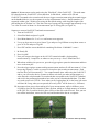
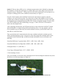
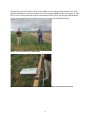
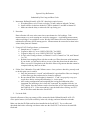
Spectral Crop Reflectance
Submitted by Dan Long and Russ Gesch
1. Instrument: Holland Scientific ACS-470 3-band active optical sensor
a. Waveband filters: red (670 nm), red edge (730 nm), and near infrared (760 nm)
b. Install red filter in detector channel #1, NIR in channel #2, and RE in channel #3.
c. Make sure that the shiny or mirrored side is up facing you.
2. Procedure:
Data collection will occur at the same time as non-destructive LAI readings. Take
measurements every week starting one week after emergence. Avoid taking measurements
when crop foliage is wet with dew or rain. Weekly NDVI data will lend to determination of
radiation use efficiency (RUE) among species. Measurements do not need to be taken in the
winter when plants are dormant.
3. Using ACS-470 Config software, set instrument:
a. Sample rate to “1 smp/sec”.
b. Vegetative Index #1: set to “NDVI (CH2,CH1)” for NDVI.
c. Vegetative Index #2: set to “NDVI (CH2,CH3)” for NDRE.
d. In CAL tab of Config software, set Channel 1 to 670, Channel 2 to 760, and Channel
3 to 730.
e. Refrain from swapping filters with the second set of filters that came with instrument.
If you do this, you will not be able to use any of the data from when the other three
filters were used. Going back to the first three filters will generate data that cannot be
compared with any other set of data.
4. Follow User’s Manual to Zero and Calibrate sensor. Once you have done this, you only need
to do this again once in a while.
a. Once the instrument is “zeroed” and calibrated it is good until the filters are changed,
or if the filters get dirty and need to be cleaned or replaced.
b. Be sure that the filter wavelengths for channels 1, 2, and 3 are properly set up (see
step d above before zeroing and calibrating (i.e., sensor span).
c. After setting configurations and completing the zeroing and calibration of the
instrument, the last thing to do is check the “Autosend” box and then click the “set
CFG” button. Now the software can be closed and the ACS-470 disconnected from
the FieldCAL SC-1. If the Autosend box is not checked before clicking “set CFG”
the ACS will not send data to the GeoSCOUT.
5. Use in the field:
Spectral reflectance of the crop canopy will be measured with the Holland Scientific ACS-470
active optical sensor (AOS) with sensitivity in the red, red edge, and near infrared wavebands.
Make sure that the SD Flash card has been installed in the GeoSCOUT. Try to collect and
download data before collecting real data to make sure the GeoSCOUT can write to the small SD
flash card.
1 Option 1: Measurements can be made using the “Plot Mode” of the GeoSCOUT. This mode must
be selected when the GeoSCOUT is first turned on. In Plot Mode, with the ACS-470 and
GeoSCOUT mounted to the extension rod, the user triggers a measurement using the manual trigger
on the handheld device (see the sequence to use for measurements below). Sample numbers are
sequential within a plot. Within a plot, using the Plot Mode setting, walk along the length of the
plot holding the ACS about 2 to 3 feet above the top of canopy taking a sample approximately every
3 to 4 feet for a total of about 6 to 10 measurements per 25-ft long plot (see Figure A).
Sequence to turn on GeoSCOUT and make measurements”
1. Turn on GeoSCOUT
2. Select Plot Mode and press Log/OK
3. Press Menu button for ~2 or 3 sec. until menu screen appears
4. Use up or down arrows to go to Sensor Type and press Log/OK then use up/down arrows to
go to ACS-470 and press Log/OK
5. Press ESC and the screen should look something like below: N:000000 V: some #
1. M: Ready P:0
6. Press Log/OK
7. Now you can press the trigger on the ACS-470 extension handle o begin making
measurements @ 1 sample/sec or whatever rate you set up. Also, P should now be 1.
8. When done with the plot you are on, press the trigger again to pause the instrument and then
move to the next plot.
9. Press the trigger again to resume making measurements and now P will increment to 2. Just
keep using sequence 7 and 8 as you move from plot to plot to make measurements. Each
time the Plot # will increment by 1. You cannot annotate plots while using the GeoSCOUT
and so you will need to devise a pattern to follow each time you make measurements (or
write down the real plot number in a notebook that corresponds to the GeoSCOUT number)
and stick in the treatment plot numbers later after you have downloaded the data. The data
are saved as an Excel CSV file. Note: when you are logging data, M: in the lower left corner
will show M: Long; when you are paused, the word “pause” will be shown (i.e., M:Pause).
10. Important: when you are done making all of your measurements, while in M:Pause, press
Log/OK to close the file (when this is done, the data, which are in flash memory are written
to the CSV file; if you don’t do this, there will be no data file on the SD card. Now you can
turn off the instrument, remove the SD card, and download the data to a computer. Figure A. Stock extension rod used to hold the instrument away from the observer and over the crop canopy. 2 Option 2: If the user has a GPS receiver, continuous measurements can be obtained by connecting
the instrument’s GeoSCOUT data logger to a suitable GPS receiver and setting to the GeoSCOUT
(using the menu) to “Map Mode”. In map mode, the AOS will be mounted to a pole and passed over
each plot at walking speed to make continuous measurements (see Figure C).
Press the “Pause” button on the GeoSCOUT at the end of a plot and press again to restart the
readings as you walk into the next plot. This action places a space in the datafile, which is used by
our data entry workbook to delimit the readings between plots. The GeoSCOUT records values from
the instrument into a comma delimited text file (CSV) in order of longitude, latitude, elevation, GPS
time, NDVI, NDRE, Red, NIR, and Red Edge. See pages 17 and 18 of the ACS-470 manual to
observe the data output format.
After completing measurements, the SD Flash Card can be removed from the GeoSCOUT and the
data downloaded to a computer using an SD card interfacing device. On your computer, open an
Excel spreadsheet (use our data entry work book) and then search for your SD Flash card to view
data and save to the Excel sheet.
These spectral data can be imported into the data entry workbook and used to calculate spectral
indices deemed important to crops. Various two or three band, single and combined indices can be
computed from the Red, Red Edge, and NIR wavebands and include, but are not limited to, the
following:
Normalized Difference Vegetation Index: NDVI = (NIR – Red) / (NIR + Red)
Normalized Difference Red Edge Index: NDRE = (NIR – RE) / (NIR + RE)
Chlorophyll Index: CI = (NIR / RE) – 1
Crop Canopy Chlorophyll Index: CCCI = NDRE / NDVI
6. Pole mounting of sensor:
The system includes an extension rod for mounting the AOS and extending the instrument away from
the observer over the crop canopy (see Figure A).
Figure B. Close up view of Crop Circle handheld system including sensor, GeoSCOUT, and extension rod
3 Alternatively, the ACS can be bolted to the middle of a wooden pole by means of two 0.25 inch mounting holes in the instrument’s base and a right angled bracket (see Figure C). The GPS receiver is also mounted near the instrument. In this set up, two people hold each end of the pole and walk the instrument over the crop canopy of an individual plot. Figure C. Crop Circle mounted on a wooden pole Figure D. Close up of mount, GPS receiver is mounted by means of Velcro seen just below the ACS-­‐470 4 Poor Stand Adjustments (added 5-­‐30-­‐2013) 1. Uniformly poor stands: plants are spread out across the plot with bare ground in between the individual plants a. Take measurements according to the protocol above. The measurements will reflect the bare soil seen through the poor canopy. 2. “Cluster” stands: Plants are grouped in “clusters” around the plot with bare ground in between the clusters. a. Visually estimate the ground cover for each plot. b. Take point measurements of the clusters. 3. Take a photograph of each plot so that we could post those on our website for the
projects.
Distance Single wavebands are sensitive to the distance between an active sensor and the crop canopy. Accordingly, the inverse square law says that the intensity of light is proportional to the inverse square of the distance from the light source. In this case, it is important to ensure that the sensor is held the same distance over each crop so that the light readings of a measurement session are comparable. Spectral indices that use two or three wavebands automatically correct for changes in distance between the sensor and crop canopy. This is because both wavebands are affected similarly. Distance studies show that vegetation indices are quite constant over a range of distances with the CropCircle sensors. 5