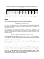
1
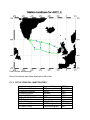
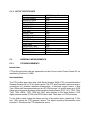
Last Update: 2000.06.26
C.1
CRUISE NARRATIVE
C.1.1
HIGHLIGHTS
Expedition Designation
74AB62_1
WOCE Line Designations AR07E, AR12
Chief Scientist:
W. John Gould
Formerly IOS Wormley but now at
Southampton Oceanography Centre
Empress Dock
Southampton, SO14 3ZH, UK
Telephone 44 1703 596208
Fax
44 1703 596204
email
[email protected]
Ship:
RRS Charles Darwin
Ports of Call:
Barry, S.Wales to Troon, Scotland.
Cruise Dates:
1 August 1991 to 4 September 1991.
C.1.2 CRUISE SUMMARY
Cruise Track
The outbound cruise track extended from south of Ireland to Cape Farewell, Greenland,
and the inboard track returned to the UK north of Ireland. Two north-south tracks linked
these lines.
Number of stations
A total of 96 CTD/Rosette stations were occupied using a General Oceanics 24 bottle
rosette equipped with 24 10-liter Niskin water sample bottles, and a NBIS Mk IIIa CTDO
instrument with Sea Tech Inc. 1m path transmissometer and IOS DL 10kHz pinger. 3 stns
(No. 79-81) were occupied using a NBIS Mk V CTD.
Sampling
The following water sample measurements were made: salinity, oxygen, total nitrate,
silicate and CFCs 11, 12, 113. NOTE THAT NO PHOSPHATE MEASUREMENTS WERE
MADE.
Float, Drifters and Moorings
None of the above items were launched on this cruise.
C.1.3 LIST OF PRINCIPAL INVESTIGATORS
Name
P.Saunders/M.Brandon
S.Bacon/M.Hartman
S.Holley/R.Paylor
S.Holley/R.Paylor
D.Smythe-Wright/S.Boswell
R.Tiddy
J.Gould/L.Povey
K.Heywood/M.Hartman
J.Gould/L.Povey
Responsibility
CTD
Salinity
Nutrients
Oxygen
CFCs
Meteorology
XBTs/Bathymetry
ADCP/Navigation
Thermosalinograph
Affiliation
SOC/BAS
SOC
SOC
SOC
SOC
SOC
UEA/SOC
SOC
C.1.4 SCIENTIFIC PROGRAMME
The WOCE Implementation Plan (World Climate Research Programme, WCRP-11 and
12, WMO/ICSU 1988) calls for the observation of the gyre scale circulation of the N
Atlantic by means of the occupation of a series of CTD station grids that have come to be
known as Control Volumes. The rationale for this observational strategy has its origins in
the observations of Armi and Stommel, 1977 (Journal of Physical Oceanography 13,828857) who observed changes in the shape and strength of the eastern Atlantic subtropical
over a period of several months.
The cruise described here is the first occupation of one such Control Volume. The data
set collected will be used to:
a) determine the changes in distribution and physical and chemical characteristics of
water masses in the area from previous surveys, notably TTO.
b) to determine the "ages" of the water masses by the measurement of CFC
concentrations.
c) to collect a data set that would enable the absolute transport of water masses through
the area to be determined together with the fluxes of heat and salt, across the area
between the UK and Greenland.
d) to make high quality meteorological measurements from the vessel using the IOSDL
Multimet package.
e) to carry out biological sampling in order to determine the relationship between ADCP
backscatter strengths and biomass distribution.
C.1.5 REPORTS AND PUBLISHED RESULTS FROM THE CRUISE.
RRS Charles Darwin Cruise 62 01 Aug - 04 Sep 1991 CONVEX-WOCE Control Volume
AR12. Cruise Report No 230 1992 IOS Deacon Laboratory, 60pp.
Hartman, M. 1992. Shipboard ADCP observations during RRS Charles Darwin Cruise 62.
IOS Deacon Laboratory, Report No. 298, 27pp.
Read, J.F. and W.J. Gould 1992. Cooling and freshening of the subpolar North Atlantic
since the 1960s. Nature, 360(6399), 55-57.
Bacon, S. 1997. Circulation and fluxes in the North Atlantic between Greenland and
Ireland. J. Phys. Ocenogr., 27(7), 1420-1435.
C.1.6 LIST OF PARTICIPANTS
GOULD W John
BACON Sheldon
BOSWELL Steve
BRANDON Mark
GWILLIAM Pat
HARTMAN Mark
HEYWOOD Karen
HILL Andy
HOLLEY Sue
JONES Doriel
PAULSON Chris
PAYLOR Rodger
POVEY Lara
READ Jane
SAUNDERS Peter
SMYTHE WRIGHT Denise
TIDDY Raoul
WOODLEY Colin
SOC (Principal Scientist)
SOC
SOC
BAS
SOC
SOC
UEA
RVS
SOC
RVS
RVS
SOC
SOC/Univ Surrey
SOC
SOC
SOC
SOC/Coventry Polytechnic
RVS
C.2
UNDERWAY MEASUREMENTS
C.2.1
CTD MEASUREMENTS
Introduction
CTD profile and bottle data are presented from the Convex cruise Charles Darwin 62, as
reported by Gould et al. (1992).
Instrumentation
The CTD profiles were taken with a Neil Brown Systems MkIIIb CTD, mounted beneath a
General Oceanics 24 by 10 litre bottle rosette. The CTD was fitted with a pressure sensor,
conductivity cell, platinum resistance thermometer, a dissolved oxygen sensor, a Sea
Tech 100cm path transmissometer and an IOS 10kHz pinger. At various times up to 8 SIS
(Sensoren Instrumente Systeme) digital reversing thermometers (RVS: T213, T220, T254,
T260, T262; IOSDL: T204, T399 and T400) were attached to the Niskin bottles. 2 SIS
digital pressure meters (6132H and 6075S) were used. There was no CTD fluorometer.
For the bottle rosette system the bases and tops of the bottles were, respectively, 0.75m
and 1.55m above the CTD pressure sensor. The digital reversing thermometers were
mounted 1.38m above the CTD temperature sensor.
Data Acquisition
Lowering rates for the CTD package were generally in the range 0.5-1.0ms-1 but could be
up to 1.5ms-1. CTD data were logged at 16 frames per second. The CTD deck unit passes
raw data to a dedicated Level A microcomputer where 1 second averages are assembled.
During this process the Level A calculates the rate of change of temperature and a
median sorting routine detects and removes pressure spikes. This data is sent to the
Level B for archival. The data are then passed to a Level C workstation for conversion to
Pstar format and calibration.
Water samples were acquired on the up cast with the winch stopped. The CTD data
acquisition system sends out a bottle firing code at the time of bottle firing. The code is
logged as serial data by the Level A which timestamps its arrival.
A total of 96 stations (01 – 96) were occupied, of which 93 used the MkIIIb CTD. A Neil
Brown MkV CTD was used at 3 of the stations. Data for stations 79-81 are from full depth
casts using this instrument. Two trials had previously been conducted at stations 72 and
76.
Data Processing
CTD Data
The 1 second data passed to the Level C were converted to Pstar format and initially
calibrated with coefficients from laboratory calibrations. The up cast data were extracted
for merging with the bottle firing codes, on time, thus the CTD variables were reconciled
with the bottle samples. Final calibrations were applied using the sample bottle data.
Pressure
A pre-cruise calibration, on 10th July 1991, using 14 points covering 0 to 5500db was:
p (dbar) = 0.997069 x praw + 4.091E-7 x praw2 – 7.31
at a temperature of 20°C. The goodness of fit was 1.0db. The calibration was made under
increasing pressure and therefore applies strictly to the down cast.
A post-cruise calibration, on 24th June 1992, shows a shift of order 4db over the year.
The following correction was applied for the effects of temperature on the pressure
sensor:
pcor = p – 0.39 (Tlag – 9)
where T lag is a lagged temperature, in °C, formed from the CTD temperature using a first
order equation with a time constant of 400 seconds. The time constant and the
temperature sensitivity of the pressure offset, 0.39°C/db, were determined from laboratory
measurements. The use of the default reference temperature (9°C) was maintained from
previous cruises.
On the up cast, a further correction is made for the hysteresis of the pressure sensor
based on laboratory measurements. For a cast in which the maximum pressure reached is
pmax dbar, the correction to the up cast CTD pressure (pin) is:
pout = pin – ( dp5500(pin) – ( (pin/pmax) x dp5500(pmax) ) )
where dp5500(p) is the hysteresis after a cast to 5500db.
A significant difference was noticed between the digital reversing pressure meters and the
CTD. The CTD pressure sensor readings at the bottom of the cast were converted to
depth and added to the height above bottom measured by the 10kHz pinger. These
compared well with Carter corrected echo sounder measurements, confirming the
calibration of the pressure sensor.
Temperature
The pre-cruise temperature calibration, obtained on 8th July 1991, was applied:
T (°C) = 0.99865 x (0.0005 x Traw) – 0.0162
The goodness of fit (over a temperature range of 0.8°C to 25°C) was 0.4mK.
Temperatures are given on the ITS90 scale. For the purpose of computing derived
oceanographic variables, temperatures were converted to the 1968 scale (T68 = 1.00024
T90).
The post-cruise calibration, on 10th January 1992, was:
T (°C) = 0.99871 x (0.0005 x Traw) – 0.0156
In order to allow for the mismatch between the time constants of the temperature and
conductivity sensors, the temperatures were further corrected according to the procedure
described in the SCOR WG51 report (Crease et al. 1988). The time constant used was
0.25s giving a correction of:
T = T + (0.25 x ∆T)
where ∆T is the change in temperature over one second calculated by the Level A.
A comparison of the CTD temperatures with the SIS digital reversing thermometers gave
the following differences:
Differences in temperature (corrected) between reversing thermometers and CTD
(Tctd-Tnnn)
Thermometer
Number
Mean diff mK
Std dev mK
T400
71
-5.5
2.5
T399
80
-8.2
1.7
T262
66
-10.9
8.1
T260
60
-10.9
4.5
T254
33
-0.7
1.5
T220
69
-9.6
10.0
T219
63
-8.2
3.2
T213
64
-7.4
9.9
The CTD temperatures were taken to be correct given their frequent calibration against
triple point cells whereas the reversing thermometers use the original manufacturer’s
calibration. The reversing thermometers are also in shallower water than the CTD sensor.
Salinity
Raw conductivities were scaled to physical units using the relationship:
C (mmho/cm) = CR x (0.001 x Craw)
The choice of conductivity ratio (CR) was made to produce salinities that were
approximately correct after comparison with bottle samples on the first few stations. CR
was found to be 1.0000.
The conductivity is then corrected for the effects of pressure and temperature in the
manner described in the SCOR WG51 report (Crease et al. 1988) with nominal values
employed for the temperature expansion and pressure contraction coefficients of the
material of the cell:
Cnew = Cold x cfac x (1 + (Cpslope x p) + CTslope x (T – Torg)
where cfac (cell factor) = 0.99856, Cpslope = 1.5 x 10⁻⁸, CTslope = -6.5 x 10⁻⁶ and Torg =
15°C. Salinity for both the down and up casts was then calculated from the corrected
temperature, pressure and conductivity.
For each station the differences between the bottle sample salinities (Sbot) and the up cast
CTD salinity (Sctd) were calculated. A routine was used to derive coefficients for the
relationship:
Sbot – Sctd = a + (b x press) + (c x potemp)
The derived a, b, c coefficients were then used to correct all CTD salinities for both the up
and down cast. Small residual errors remained between the corrected salinities and the
bottle values that were a function of depth. These resulted in salinities that were high by of
order 0.001 in depths greater than 2500m. Similarly salinities were low by a similar
amount between 1200 and 1700m. The errors were more scattered above 500m due to
the uncertainties created by the stronger salinity gradients.
Oxygen
The CTD oxygen sensor data were calibrated against bottle samples. No further details
are available.
Transmittance
No calibration details are available for the transmissometer.
Sample Data
Chlorofluorocarbons
Samples for CFC compounds were always the first to be taken from the Niskin bottles.
Analyses were conducted using 2 gas chromatographs, one belonging to JRC (for CFC11 and CFC-12 measurements) and the other to PML (for additional CFC-113 analysis).
Electron Capture Detection (ECD) was used to remove dissolved gases from the seawater
sample, separate the compounds, and measure their concentration. The ECD was
calibrated using a standard gas with a known fraction of each compound.
The CFC-113 data are considered suspect due to problems with the PML system. The
data were not made available to BODC and are not presented here.
Oxygen
Samples for dissolved oxygen analysis were taken from the Niskin bottles after the CFCs.
Samples were drawn into weight calibrated 120ml narrow necked glass bottles fitted with
ground stoppers. The pickling reagents were added on deck immediately after drawing
and before capping.
Analysis was performed in a constant temperature laboratory at 21°C using the Carpenter
modifications (Carpenter, 1965) (with the exception of the thiosulphate titrant which was
made up to a concentration of 0.2M) of the Winkler technique with an automated
photometric endpoint detection system. This consisted of a solid state light source and
photodiode detector peaked to the iodine signal, a Metrohm dossimat, and a PC and
software supplied by Sensoren Instrumente Systeme. Blanking was performed using pure
water and not seawater to avoid differences due to depth and position. Equations
specified in the WOCE Operations and Methods manual (Culberson, 1991) were used to
calculate the oxygen concentrations. A buoyancy factor was applied to the weight of the
potassium iodate standard.
Precision was monitored by taking two or more duplicate samples from each cast. With
the exception of stations 12 through 25, where a small air lock in the equipment caused
reproducibility problems, the standard deviation of all duplicates was calculated to be
0.007ml/l which equates to 0.1% full scale. For stations 81 to 83 there was a periodic
blockage in the aspirator which caused some of the titrations to fail.
Nutrients
Sampling for nutrients followed that for CFCs and dissolved oxygen. Samples were drawn
directly into 30ml transparent high density polyethylene diluvials fitted with press on caps.
Samples were analysed for nitrate and silicate using an Alpkem Corp. Rapid Flow
Analyser, model RFA 300. The RFA system was sited in the constant temperature
laboratory and the analysis temperature was 21°C throughout the cruise.
Phosphate measurements were also planned, however, the capped head on the non-toxic
seawater supply in the constant temperature laboratory blew when the water supply was
turned on. This resulted in the autoanalyser being flooded and damaged an electronic
board in one of the photometer units and an air phase injection board on the pump
assembly. This rendered one of the autoanalyser channels unserviceable and it was
decided to sacrifice phosphate analysis.
The method for nitrate was that given in the Alpkem manual (Alpkem Corp., 1987) and
involving the initial reduction of nitrate to nitrite by cadmium, in the form of an open tube
cadmium reactor. Following diazotisation with sulphanilamide and coupling with naphthyl
ethylene diamine dihydrochloride to form an azo dye, total nitrite was measured at an
absorbance maximum of 543nm. Interferences from metals were eliminated by the use of
an imidazole buffer solution.
The method for silicate involved the addition of ammonium molybdate at acidic pH to
produce b molybdosilicic acid, which was then reduced using ascorbic acid to form an
intensely blue molybdenum complex with an absorbance maximum of 820nm.
Interferences from phosphomolybdate and arsenomolybdate formed during the initial
stages of the reaction were eliminated by decomposition with oxalic acid. The method
employed was an adaptation of the Alpkem method given in the manual because it had
been noted that slight temperature fluctuations markedly affect analytical precision and
accuracy. To overcome this a 2ml mixing coil place in a heating bath at 37°C was inserted
before the flow cell of the original cartridge. By inserting the heated coil the chemical
reaction and hence colour development was allowed to proceed to completion before
measurement.
Listed below are the reagents used for analysis; stock 10mmol/l solutions of sodium
hexafluorosilicate (0.96g) and potassium nitrate (0.505g) were used to standardise the
analyses.
Nitrate + Nitrite:
Imidazole Buffer
Combined reagent
Sulphanilamide
Hydrochloric Acid
Brij 35
N.E.D
Silicate:
Combined reagent
Ammonium Molybdate
Sulphuric Acid
Sodium Dodecyl Sulphate
Oxalic Acid
Ascorbic Acid
6.81 g/l
5 g/l
100 ml/l
30% w/v
1 g/l
10.8 g/l
2.8 ml/l
15% w/v
10% w/v
18 g/l
pH 7.5
10 ml/l
20 ml/l
The autoanalyser was calibrated using a six point standard curve. Mixed nitrate/silicate
standards were prepared daily in artificial seawater from the stock 10mmol/l solutions. The
standards ranged from 0 – 30mmol/l for nitrate and 0 – 50mmol/l for silicate and were
evenly spaced throughout the concentration range. Three individual stock standards of
nitrate and silicate were prepared during the cruise.
Precision was assessed by analysing replicate samples taken from the same Niskin bottle.
Two replicate samples were taken at random from each cast and analysed on the same
analytical run. Precisions based upon duplicate measurements were calculated by
working out the standard deviation of duplicate pairs and expressing the figure as a
percentage of the concentration of the highest standard. Precision for silicate was 0.15%
and for nitrate 0.53%.
Accuracy was assessed on one occasion using commercially available standards supplied
by the Sagami Chemical Company of Japan. The values obtained for these standards
were found to be within 0.1% of the 10mmol/l silicate and 0.5% of the 15mmol/l nitrate
values quoted by the manufacturer. These standards were prepared in a similar matrix to
the calibration standards.
Salinity
Salinity samples from the Niskin bottles were analysed using Guildline 8400 bench
salinometers (an old 8400 – first half of cruise, and a new 8400A – latter half) set to run at
24°C in the temperature controlled laboratory (22°C). Standardisation was done using
IAPSO Standard Seawater batch P115.
The standard deviation of 200 pairs of duplicate samples was 0.001psu.
Oxygen and Hydrogen Isotope Ratios
Samples were collected into 250ml salinity bottles. The bottle necks were covered with a
sheet of aluminium foil and the lid screwed on tight. Care was taken not to rip the
aluminium foil because this acts as a water impermeable barrier to prevent contamination.
Delta oxygen-18 of water was measured using a mass spectrometer. No analyses were
conducted for hydrogen isotope ratio.
Reversing Thermometers
8 SIS digital reversing thermometers were attached to the Niskin bottles.
BODC Data Processing
No further calibrations were applied to the data received by BODC. BODC were mainly
concerned with the screening and banking of the data.
CTD Data
The CTD data were received as 2db averaged pressure sorted down cast data. The data
were converted into the BODC internal format (PXF) to allow the use of in-house software
tools, notably the graphics editor. Spikes in the data were manually flagged ‘suspect’ by
modification of the associated quality control flag. In this way none of the original data
values were edited or deleted during quality control. These data from cruise CD62
required little flagging and just a few points were set suspect.
Once screened, the CTD data were loaded into a database under the Oracle relational
database management system. The start time stored in the database is the CTD
deployment time, and the end time is the time the CTD was removed from the water.
Actually these times are more precisely the start and end of data logging. Latitude and
longitude are the mean positions between the start and end times calculated from the
master navigation in the binary merged file. The longitude given to the end time for station
62 in the cruise report is incorrect and should be closer to –35° 50.0.
Sample Data
BODC conducted extensive quality control to eliminate rosette misfiring and any
incorrectly assigned flag codes. Before loading to the database the data were averaged if
bottles fired within ±4.0db of each other. For stations 19, 21 and 42 a bottle entry exists at
a pressure greater than the maximum CTD pressure. This is most probably due to the
CTD casts having been edited by the originating scientists. No bottle data were received
for station 96.
References
Alpkem Corp. (1987). Operator's manual, RFA 300. Clackamas, Oregon. Unnumbered
loose leaf pages.
Carpenter, J.H. (1965). The Chesapeake Bay Institute technique for the Winkler dissolved
oxygen method. Limnol. Oceanogr., 10, 141-143.
Crease, J. et al. (1988). The acquisition, calibration and analysis of CTD data. UNESCO
Technical Papers in Marine Science. No. 54, 96pp.
Culberson, C.H. (1991). Dissolved oxygen. WOCE operations manual WHPO 91-1.
WOCE Report No. 68/91.
Gould, W.J. et al. (1992). RRS Charles Darwin Cruise 62. Institute of Oceanographic
Sciences Deacon Laboratory, Cruise Report No. 230, 60pp.
C.2.2 SAMPLE SALINITY DETERMINATIONS (SB)
Both IOSDL Guildline Autosal salinometers, the old one (model 8400) and the new one
(model 8400A) were carried on this cruise and operated at 24 degC in the Darwin
constant temperature laboratory, which was maintained at 22 degC. The former was
operated for the first half of the cruise and the latter for the second half. Both machines
showed unusual stability of standardisation, neither deviating from their original values by
more than 0.001 equivalent salinity. The old machine was initially preferred over the new
one because the latter showed a large change in standardisation over the value at which it
left IOSDL. This may be attributable to knocks suffered during transportation to Barry; it
did not affect the machine's subsequent performance. Towards the end of the cruise, a
fault developed on the FUNCTION switch on the new machine which resulted in display
instability in the standby (SBY) position. This will need to be rectified upon return.
Previous operational difficulties associated with the new machine, in particular its
instability when run from a noisy power supply, have been rectified; no difficulties on this
count were experienced.
About 1800 CTD bottle samples and 200 samples drawn from the ship's non-toxic supply
(for thermosalinograph calibration) were processed during the cruise. 200 pairs of
duplicate samples are included in the CTD sample figure, for which the standard deviation
of the difference between salinities was 0.001. Only one pair of duplicates was more than
0.002 different. 250 ampoules of standard seawater BATCH P115 used throughout were
consumed.
The data processing route was changed during the cruise. Initially, the Ocean Scientific
International 'Salinity' program was used to generate files of salinity data on an IBM PS-2,
which were transferred to an Apple Macintosh, edited as a Microsoft Word text file and
then transferred to the shipboard SUN system. Latterly, the data were entered directly
into an Excel spreadsheet program on a Macintosh into which was pasted the approved
conductivity ratio to salinity conversion formula. After testing and comparison, the Excel
system was used exclusively. This was more efficient; a text file saved from Excel could
be transferred to the SUN with no requirement for intermediate stages of processing.
C.2.3 CHEMISTRY OVERVIEW (DS-W,RP,SMB,SH)
The primary aim of the chemistry work was to collect a narrowly spaced data set to the
precision and accuracy required by the WOCE Hydrographic Programme (WHP) in order
to chemically characterise and age the water masses of this area of the North Atlantic.
The data would subsequently be used for flux measurements and to calculate transport
rates within the subpolar gyre. Measurements of CFCs were planned at as many
locations as possible (limited by the rate at which samples could be analysed) and of
oxygen and nutrients at each station. Samples were collected for oxygen and hydrogen
isotope measurement by NERC Isotope Geosciences Laboratory (NIGL).
The CONVEX survey provided the first opportunity for comprehensive measurement of
CFCs in both western and eastern basins of the subpolar gyre. Because much of the
water in the area is relatively new (i.e. was at the surface less than a decade ago) it was
thought that the CFC-12/CFC-11 technique widely used within the WHP would not give
sufficient information (the ratio of CFC-12/CFC-11 upon which the ageing technique is
based has not changed much for more than a decade and so it can be difficult to age with
any precision over this time period), and so measurements of the new CFC tracer, CFC113 were planned.
In contrast the ratio of CFC-113 to either CFC-11 or CFC-12 has
changed substantially in the past decade. However, provided little or no mixing has taken
place, it is possible to age core water mass with some reliability over the last 15 years
using CFC-11 and CFC-12 data alone, by using a combination of the ratio with absolute
concentrations. Comparison with T, S and nutrient data facilitates this ageing technique.
Ageing from CFC-113 data is very new and requires some further development. It also
suffers from potentially severe CFC-113 contamination problems; a problem which also
hampers CFC-11 and CFC-12 measurements but to a lesser extent provided the research
vessel does not contain these substances within its air conditioning and refrigeration
systems. Since two CFC systems were taken to sea, one belonging to the JCR (for CFC11 and 12 measurements) the other to ML (for additional CFC-113 analysis) the cruise
provided an opportunity for intercalibration of the two systems. It had been hoped that the
JRC system would be upgraded for CFC-113 measurement prior to the cruise but due to
late delivery of a number of components this was not possible.
Like
the
CFCs,
oxygen measurements are indicative of water which has recently left the surface and are
usually enriched in cold polar waters such as the overflow through the Denmark Strait.
The nutrients nitrate, phosphate and silicate compliment CFC and oxygen measurements
in that water masses are often high in one and not in another. A combination of all
measurements results in distinct fingerprinting for many of the oceans water masses.
Oxygen and hydrogen isotope measurements can be used as oceanographic tracers and
have been used successfully for tracing waters with a polar origin. Both have heavy
isotopes that are fractionated from their lighter more abundant counterparts during
processes of evaporation and precipitation, where they are more concentrated in the liquid
phase, and during freezing where the ice becomes enriched over the mother liquid. On
melting the high levels of O18 and H2 remain and make them a useful tracer for assessing
the amount of ice melt in a particular water mass. Most of the tracer work to date has
been at high latitudes, very little has been carried out in the subpolar area. Furthermore
the technique for oceanographic tracer use is new in the UK. The cruise provided the
opportunity to collect samples for a combined investigation with NIGL for assessing
analytical techniques and usefulness of such data at lower latitudes.
The cruise also gave an opportunity to evaluate the workload, personnel requirement and
sample handling and analysis techniques for the forthcoming WOCE WHP A-11.
Sample collection
All samples were collected from depth using the IOSDL 10 litre Niskin bottles. These had
been cleaned prior to the cruise using a high pressure water jet. All O-ring seals and taps
were removed, washed in decon solution and propan-2-ol then baked in a vacuum oven
for 24 hours. Cleaning and reassembling of the bottles was carried out just prior to the
cruise to minimise contamination due to long storage. 54 bottles were taken to sea in
case of contamination or damage, but only 24 where used. All bottles, whether in use or
not, remained on deck throughout the cruise. None of the 24 working bottles showed a
CFC contamination problem during the entire cruise.
C.2.4 CFCs
The bulk of the CFC measurements were made using the JRC CFC system. Samples
from 85 stations were analysed immediately after collection for CFC-11 and CFC-12. Due
to the close station spacing and the required analysis time it was not possible to sample
the full range of depth levels at all stations. When turn-over time was limited, sampling
was concentrated on the deepest depth levels. (Data on number of samples taken on
each station is given elsewhere in the CTD station list).
In general the JRC system worked extremely well. Only two mishaps occurred, both due
to the extreme weather. First the cooling bath fell off the bench during a particularly bad
roll and this fractured the flexible pipe. It was quickly removed from the laboratory so as
not to contaminate the CFC equipment and replaced with a spare. No downtime resulted.
The second problem started with a noisy baseline from the ECD in the gas
chromatograph. The problem became substantially worse, rendering the system useless
for measurement and eventually the signal died altogether. In the first instance, there
appeared to be a correlation with the roll of the ship and so it was presumed that a wire
had worked free due to the inclement weather. It was not possible to verify this because
of the need to open the radioactive detector and JRC/IOSDL do not have a licence for
such work. Fortunately the JRC system is fitted with a spare ECD and so this was brought
on line and the system functioned perfectly for the remainder of the cruise. Approximately
eight hours downtime resulted from this problem, with the loss of one station.
The PML system seemed dogged with problems from the outset. The computer running
the calibration and data storage programs was not available due to failure on a previous
cruise. Backup software was supplied with the system but this was not comprehensive.
During set up one of the valve controllers failed and had to be rewired. This was shortly
followed by one of the valve actuators burning out, and since no spare was supplied this
meant the valve V4 had to be turned manually. Once set up the system developed a
baseline oscillation that rendered data collection useless. Although various theories
where tested and advise sought from PML, the reason for the fault was not established.
After about 2 weeks at sea the system cured itself following particularly inclement weather
and a time when the cryocool was not operational leaving the molecular sieves at ambient
temperature for a few hours. This suggested either a possible loose contact somewhere
in the system or a pressure problem that was resolved when the flow rate in the sieves
changed during heating and subsequent cooling. By this stage, however, it was decided
to concentrate on the JRC system as this was giving good results. Nevertheless work
with the PML system did continue but the chromatography was poor, with considerable
overlap of peaks. Since time and personnel were at a premium it was not feasible to
spend hours trying to obtain better separation when it was not obvious that this would
have been achieved. We therefore concluded that there remain several question marks
against the use of the PML system as a routine analytical tool.
Firstly, the
chromatographic resolution needs improving. Secondly, the system is very fragile and
requires constant attention to maintain high quality results. Thirdly, it is not robust enough
to cope with the large sample turn around required by WHP cruises.
Both CFC systems were set up in the main laboratory of the ship. From the CFC
contamination aspect, the RRS Charles Darwin is a clean vessel with results from the JRC
system suggesting no major contamination problems.
Some contamination was
experienced with the PML system but this was traced to loose gas connections and it
cleared once these had been tightened. No contamination was found from the opening of
the air conditioning unit door on the boat deck as had been suggested after Darwin 58 and
59.
CFC concentration measurements suggest that Labrador seawater and Denmark Strait
overflow water are of the order of 10 years old whereas the water at depth in the Eastern
Basin is very much older corresponding to an age of nearer 50 years.
C.2.5 NUTRIENTS
Equipment and Technique
The nutrients nitrate and silicate were measured using an Alpkem Corp., Rapid Flow
Analyser, model RFA 300 by a team of analysts from the James Rennell Centre for Ocean
Circulation. The RFA system was sited in a constant temperature laboratory and the
analysis temperature was 21C throughout the cruise.
The method for nitrate was that given in the Alpkem manual (Alpkem Corp., 1987) and
involving the initial reduction of nitrate to nitrite by cadmium, in the form of an open tube
cadmium reactor. Following diazotisation with sulphanilamide and coupling with naphthyl
ethylene diamine dihydrochloride to form an azo dye, total nitrite was measured at an
absorbance maximum of 543 nm. Interferences from metals were eliminated by the use
of an imidazole buffer solution.
The method for silicate involved the addition of ammonium molybdate at acidic pH to
produce b molybdosilicic acid, which was then reduced using ascorbic acid to form an
intensely blue molybdenum complex with an absorbance maximum of 820 nm.
Interferences from phosphomolybdate and arsenomolybdate formed during the initial
stages of the reaction were eliminated by decomposition with oxalic acid. The method
employed was an adaptation of the Alpkem method given in the manual because it had
been noted that slight temperature fluctuations markedly affect analytical precision and
accuracy. To overcome this a 2 ml mixing coil place in a heating bath at 37C was inserted
before the flow cell of the original cartridge. By inserting the heated coil the chemical
reaction and hence colour development was allowed to proceed to completion before
measurement.
Samples were not analysed for phosphate due to loss of the photometer at the start of the
cruise.
Listed below are the reagents used for analysis; Stock 10 mmol/l solutions of Sodium
Hexafluorosilicate (0.96 g) and Potassium Nitrate (0.505 g) were used to standardise the
analyses.
Silicate.
Combined reagent
Ammonium Molybdate
Sulphuric Acid
Sodium Dodecyl Sulphate
Oxalic Acid
Ascorbic Acid
Nitrate + Nitrite
Imidazole Buffer
Combined reagent
Sulphanilamide
Hydrochloric Acid
Brij 35 30% w/v
N.E.D
10.8 g /l
2.8 ml /l
15% w/v
10% w/v
18 g /l
20 ml /l
6.81 g/l
pH 7.5
5 g /l
100 ml /l
10 ml /l
1 g /l
Sampling Procedure
Sampling for nutrients followed that for CFCs and dissolved oxygen and was typically 45
minutes after the rosette was on deck. Samples were drawn directly into 30 ml
transparent high density polyethylene diluvials fitted with press on caps: each vial was
flushed with three times its volume before filling. Samples were immediately transferred to
the constant temperature laboratory and all analyses completed within an hour and a half
of collection. An exception to this was on Stations 18 and 19 when due to a malfunction of
the autoanalyser a delay was anticipated. These samples were stored refrigerated at 4C
for approximately one and a half hours before analysis. For all samples the 2.5 ml
autoanalyser polystyrene cups were rinsed with three times their volume before filling.
Calibration
The autoanalyser was calibrated using a six point standard curve. Mixed nitrate/silicate
standards were prepared daily in artificial sea-water from the stock 10 mmol/l solutions.
The standards ranged from 0 - 30 mmol/l for nitrate and 0 - 50 mmol/l for silicate and were
evenly spaced throughout the concentration range. Three individual stock standards of
nitrate and silicate were prepared during the cruise.
Precision was assessed by analysing replicate samples taken from the same Niskin bottle.
Two replicate samples were taken at random from each cast and analysed on the same
analytical run. Precisions based upon duplicate measurements were calculated by
working out the standard deviation of duplicate pairs and expressing the figure as a
percentage of the concentration of the highest standard. Precision for silicate was 0.15%
and for nitrate 0.53%.
Accuracy was assessed on one occasion using commercially available standards supplied
by the Sagami Chemical Company of Japan. The values obtained for these standards
were found to be within 0.1% of the 10 mmol/l silicate and 0.5% of the 15 mmol/l nitrate
values quoted by the manufacturer. These standards were prepared in a similar matrix to
the calibration standards.
Units used
Nutrient data were converted from mmol/l to mmol/kg units by multiplication with the
density calculated from sample salinity and a temperature of 21C; the temperature of the
constant temperature laboratory where the analyses were performed.
Data quality checks
Nutrient data quality was checked for each station by comparison of plots of nutrient
concentration versus potential temperature. Plots for consecutive stations were overlaid
to observe obvious errors such as large spikes in the data indicating contamination. For
example low silicate and nitrate values were observed for sample 23 station 41 and
accidental dilution of the sample was suspected. In such cases the data are not reported
and a flag of 5 recorded.
Drift in the data was detected in a similar way. For station 84 nitrate data shifted low but
was not further queried since it correlated with subsequent stations. Due to the wide
range of silicate values, silicate data were checked on an expanded scale where
necessary.
Where data appeared questionable analytical logsheets were scrutinised to ensure correct
standardisation procedures and reagent composition. If no explanation was obvious
further comparisons were made with nutrient concentration verses pressure plots, oxygen
profiles and topography. When no obvious reason could be found to reject the data but it
still looked unusual when plotted against potential temperature or pressure then a flag 3
was recorded. For example nitrate data from stations 75 to 78 are high but substantial
checking suggested no reason to consider the measurements as bad. However questions
still need to be addressed so the nitrate data for these stations have been flagged as 3.
Data for station 69 are flagged 4 because a blockage in the sample probe was suspected.
A flag 9 is recorded for absent data.
Comparison with historical data sets
Data accuracy was checked by comparison with historical data sets from the same area:
TTO (1981) and TYRO 90/3 (1991). The TYRO 90/3 study concentrated on the WOCE
AR7E line which also made up part of the CONVEX study area. Data comparison was
done in two ways:
Firstly, nutrient data from all of the CONVEX stations were plotted against potential
temperature on a single graph. Similar plots were prepared for the TTO and TYRO 90/3
data and the plots were overlaid. This exercise was repeated using nutrient versus
pressure plots. The CONVEX data fell within the scatter of the TTO and TYRO 90/3 data.
Secondly, four TTO stations from the same location as four CONVEX stations, were
selected and comparisons of data below 1000 m were made. Comparisons in the surface
waters were not valid due to seasonal differences and different biological activity effecting
the surface nutrient concentrations. The comparisons suggested that there was no
detectable difference for silicate concentrations but nitrates differed from TTO by up to 0.8
mmol/kg.
Overall the silicate and nitrate chemistries worked well and the data from the repeat
stations, cd62082 and cd62010, are consistent.
References
Alpkem Corp.,1987. Operator's manual, RFA 300, Clackamas, Oregon. Unnumbered
loose leaf pages.
C.2.6 OXYGEN
Equipment and Technique
Samples from the Niskin bottles were analysed for oxygen using an automated Winkler
titration unit supplied by Sensoren Instrumente Systeme. It comprises a fully automated
PC driven photometric endpoint detection method using a solid state light source and a
photodiode detector peaked to the iodine signal. The titrant is dispensed by a Metrohm
Dosimat model 665 with a 1 ml exchange unit. All reagents were made up according to
the procedures and concentrations specified by Carpenter (1965), with the exception of
the thiosulphate titrant which was made up to a concentration of 0.2M. This allowed the
titration to be performed within one single delivery of the exchange unit. The standard titre
was typically 0.500 ml, and the blank titre 1 ml. Details of equipment operation may be
found in the SIS manual (1989). All analyses were performed in a constant temperature
laboratory at 21C
Blanking and standardisation procedures were carried out at least once a day using
deionised water. All calculations were performed using the equations specified in the
WOCE Operations and Methods manual. A buoyancy factor was applied to the weight of
the potassium iodate standard.
Sampling Procedure
Samples for oxygen were taken, immediately after CFCs, directly into weight calibrated
120 ml narrow necked glass bottles fitted with ground stoppers. Sample flasks were
flushed with three times their volume prior to filling and pickling reagents added
immediately. The samples were analysed about two hours after collection to allow them
to equilibrate to the constant laboratory temperature. All analysis was completed within
three hours of the cast arriving on deck.
Calibration
Precision was monitored by taking two or more duplicate samples from each cast. Short
term precision was monitored on 92 stations throughout the cruise. With the exception of
stations 12 through 25, where a small air lock in the equipment caused reproducibility
problems, the standard deviation of all duplicates was calculated to be 0.007 ml/l which
equates to 0.1% full scale. For stations 81 to 83 there was a periodic blockage in the
aspirator which caused some of the titrations to fail.
Units
The data were converted from ml/l to mmol/l using a factor of 44.66 to convert ml/l to
mmol/l and to mmol/kg using seawater density calculated from the salinity and potential
temperature of the sample. Changes in bottle volume due to temperature effects were
considered to be minimal. Calculations on a previous cruise revealed that the change of
volume resulted in less than 0.02% change for the entire temperature range encountered
on CONVEX; for example a calculated oxygen value of 5.000 ml/l at 20C would alter by
less than 0.001 ml/l if measured at 0C.
Data quality checks
Oxygen data were checked, in a similar way to the nutrients, by comparing plots of oxygen
concentration versus potential temperature. Plots for consecutive stations were overlaid
to observe obvious errors and in such cases the data are not reported and a flag of 5
recorded. When the titration failed a flag of 4 (bad measurement) was recorded with the
absent data. Flag 9 was recorded when no sample was collected due to failure of the
Niskin bottle.
Comparison with historical data sets
Data accuracy was checked in the same way as that for nutrients by comparison with TTO
(1981) and TYRO 90/3 (1991) data. The comparison was done in two ways;
Firstly, oxygen data from all of the CONVEX stations were plotted against potential
temperature on a single graph. Similar plots were prepared for the TTO and TYRO 90/3
data and the plots overlaid. This exercise was repeated using oxygen versus pressure
plots. The CONVEX data fell within the scatter of the TTO and TYRO 90/3 data.
Secondly, four TTO stations from the same location as four CONVEX stations, were
selected and comparisons of data below 1000 m were made. Comparisons in the surface
waters were not valid due to seasonal differences and different biological activity effecting
the concentrations. The comparisons suggested that there were no detectable differences.
Data from the repeat station, cd62082 and cd62010, were compared and found to be
consistent.
References
Carpenter, J H, 1965. The Chesapeake Bay Institute technique for the Winkler dissolved
oxygen method. Limnol. Oceanogr. 10, 141-143.
SIS User Manual Version 2.01. Kiel, Germany.
WHP operations and Methods Manual, 1991.
C.2.7 OXYGEN AND HYDROGEN ISOTOPE RATIOS
A total of 165 samples were collected from 7 stations for isotope analysis. These included
6 duplicate samples for assessment by NIGL and a complete set of duplicated from
station CD0072 for analysis at UEA. The latter were requested by KH to evaluate the
UEA analytical capability. Samples were collected into 250 ml salinity bottles following an
initial rinse and two fillings and emptying method. On the third fill the neck was covered
with a sheet of aluminium foil and the lid screwed on tight. Care was taken not to rip the
aluminium foil because this acts as a water impermeable barrier to prevent contamination.
C.2.8 METEOROLOGY - THE MULTIMET SYSTEM (RJT)
Note the archived data is at the WOCE Meteorology DAC, Florida State University and
can be retrieved via http://www.coaps.fsu.edu/WOCE or from the WOCE CD-ROMs v1.0
dataset on the Surface Meteorology Disc (Atlantic). The Cruise is identified as AR7E/03.
Sensors
The sensors were situated on the foremast, mainmast, and on the port and starboard
sides of the wheelhouse top. The forward mast carried a propeller vane anemometer
(R.M.Young serial number (S/N) 6992) and a Gill sonic anemometer situated on the
forward platform. Two aspirated psychrometers (Vector instruments (VI) S/N 1066, and
S/N 1072) were situated port and starboard. The short wave radiation sensors were
situated to the far port and starboard side of the forward mast platform (Kipp and Zonnen
S/N 11902837 and 11871958). The long wave radiation sensor (Eppley S/N 27225F3)
was situated at the top of the upper foremast. On the wheelhousetop there was an
aspirated psychrometer (VI S/N 1058) situated to the port side, and also to the starboard
side (VI S/N 1060), in each case just aft of the ladder. The main mast carried an
anemometer (VI S/N 1895) and a wind direction sensor (VI S/N 2224) situated at the mast
top.
Multimet
The IOSDL Multimet system recorded data once per minute throughout the cruise. All the
data from all the sensors were recorded. Wind speed data from the mainmast
anemometer stopped transmitting data on day 233, and only transmitted intermittently
from then on.
Problems with the recorded data included a possible calibration error with the starboard
dry bulb temperature on the wheelhouse top, and the foremast anemometer data from
day 237 onwards.
For each 24 hour segment, for head to wind (foremast anemometer direction 150 to
210degT) values at night (20-24 and 0-8 hours) the mean starboard dry bulb temperature
on the wheelhouse top read a maximum of 0.32C high compared to the mean starboard
dry bulb temperature on the foremast; and a maximum of 0.28C high compared to the
mean port dry bulb temperature on the wheelhouse, (Possible calibration error). For days
213 to 242.0 the mean starboard dry bulb temperature on the wheelhouse top read 0.21C
high compared to the mean starboard dry bulb temperature on the forward mast; and
0.13C high compared to the mean port dry bulb temperature on the wheelhouse.
The starboard wheelhouse top psychrometer was effected by heat from the funnel when
the relative wind direction was between 72 degrees and 144 degrees (where 0 degrees is
the aft of the ship). The port wheelhouse top psychrometer was effected by heat from the
funnel when the relative wind direction was between 288 and 360.
Each time the wheelhouse psychrometers were filled the water in the starboard
psychrometer was considerably lower than the water in the port psychrometer. There was
no leak in the bottle, possible causes could be either funnel smoke or heat from bridge
door being open.
The foremast anemometer was seen to be at an angle (instead of horizontal) on day 237.
This did not seem to have affected its ability to transmit data. But on day 237, the relative
foremast wind direction seemed to be reading low by about 40-60 (should have been
about 350 but it read about 290), presumably due to the angle of the anemometer.
Calculation of the true wind speeds and directions from then on were incorrect, in that
when the ship changed directions a jump occurred in the true winds.
Shadowing by the foremast occasionally caused the port short wave solar radiation sensor
to read lower than the starboard short wave solar radiation sensor.
Special interest should be taken of day 229 and 230, where there was a very sudden
increase in wind speed.
Processing the Multimet Data
The time series of each sensor shown on the BBC computer were checked daily, as were
the sensors. The data was processed on the Sun in 24 hour segments. The processing
of the Multimet data used four execs (mmexec0 to mmexec3).
• mmexec0 extracts the daily meteorological data from the RVS files and applies
calibrations to it.
• mmexec1 plots the daily data.
• mmexec2 calculates the specific humidities for each psychrometer, and then calculates
the temperature and specific humidity differences for each sensor, it then calculates the
head to wind values (using the foremast anemometer data) at night to find any possible
calibration errors in the psychrometers.
• mmexec3 calculates the true wind speed and direction using the foremast anemometer
data.
Problems with the Multimet Processing
Days 213 to 221 (inclusive) the meteorological calibration file was incorrect for the gyro (it
read column one as 1, it should have read 1.4117). Thus for this period the archived data
with file names:
mm$cruise$met,
mm$cruise$met.hour,
mm$cruise$met.q3,
mm$cruise$met.qdf
the gyro is wrong. But it can be corrected by using a linear calibration of (gyro*1.4117)
using pcalib. The gyro plots for this period are therefore also incorrect, the correct gyro
plots can be seen in the true wind plots. The appended mm$cruise file thus also had an
incorrect gyro, this was corrected using pcalib and this version archived. The
meteorological calibration file was changed for days 222 onwards.
Up to and including day 225, there was a mistake in mmexec2, and the archived files
mm$cruise$met.q3 were really mm$cruise$met.q archived. From day 226 onwards the
archived files are correct.
Sonic Anemometer
The data from the sonic anemometer on the foremast was logged constantly on a PC.
This data was backed up daily on to the Sun system, when the ship was steaming so as
not to loose good data. The sonic stopped logging on day 238, but was restarted on day
239, this data was therefore not logged. Data before and after seemed to be good.
SBWR
The data from the shipborne wave recorder was logged constantly on a PC. This data
was backed up daily on to the Sun system, when the ship was steaming so as not to
loose good data. There were no problems.
C.2.9 XBT DATA (WJG,LP)
This data has been submitted to the NODC archive, Washington and can be found in the
July-Sep 1991 BEST COPY GTSPP Archive. This can be reached at the time of writing
via http://www.nodc.noaa.gov/GTSPP/gtspp-home.html or via the WOCE CD-ROM v1.0
dataset on the Upper Ocean Thermal Disc.
XBT data were obtained between the CTD stations and on some passage legs in order to
provided improved spatial resolution of mesoscale features. The shipboard system used
was a Bathysystems SEAS system transmitting data via the GOES satellite. The
equipment was suppliedand installed by the MoD Hydrographic Department.
We were supplied with a new version of the Seas system software and were sent to sea
with only very limited documentation. A fault developed in system on day 224 that
indicated that the GOES buffer was not being cleared and that the real time data were
probably not being transmitted to the satellite. The problem was not traced until day 234
when contact with MoD through RVS revealed that the power supply that was charging
the batteries was not working. The problem was rectified and thereafter no problems were
encountered. In future the vessel should carry a complete handbook of hardware and
software documentation.
The new software has a number of annoying faults
a) the logged time for an XBT is the time at which the programme is set up. Previous
versions have used the much better system of attributing the drop time to the time
when the probe is launched, clearly much better and sometimes up to 10 minutes later
than the setup time with consequent errors in position.
b) A most annoying feature is the format for entering positions. A <return> is required for
the numerical value but not for the N/S E/W entry. Similarly a 3 digit degree entry is
required for longitude and an entry of 2 or less (e.g. 16 rather than 016) leads to errors.
c) When the water depth is less than the probe's maximum depth the programme asks
whether a shallower cutoff is required. It would be much better to ask the operator to
specify a cutoff level after the profile is complete so that a partial trace can be
transmitted.
d) There is no way to dump the plot of the profile to the printer, a serious omission, and
no way to dump data except at the raw data rate. You would like to be able to list data
every say 10 or 20 metres and to specify the particular isotherms for which depths are
required rather than just whole degrees.
The probes used were Sippican T-7 and T-5 and Plessey T-7. Few probes failed and
these can be attributed largely to problems with the XBT software, a leakage in the
launcher cable and to the XBT wire fouling the ship in the often poor weather. This latter
problem was helped by the use of a length of plastic tubing that fitted over the probe
canister. In rough weather probes could not safely be launched from the stern and so
they were often deployed near the hatch in a relatively sheltered position. This seemed to
work well. Some T-5 probes were launched at too high a speed early in the cruise and
these are noted in the XBT table.
Data were transferred from the PC floppies to the PSTAR system using a programme
written on board by Doriel Jones. No transfer software nor indeed any information on PC
file formats was supplied. The data were subsequently edited in PSTAR to remove spikes
and near surface transients.
The temperatures matched well to the thermosalinograph values.
C.2.10
THERMOSALINOGRAPH (WJG, LP)
The thermosalinograph was based on Sea Bird temperature and conductivity sensors
mounted in an enclosure in the Hydro Lab. The data together with the sea water intake
temperature were logged on the RVS computer system and later transferred to PSTAR.
Calibration samples were taken at two hourly intervals from the outflow from the
thermosalinograph housing. These were analysed and the data for the whole cruise
plotted. A rather constant offset was seen until day 230 after which time the offset
decreased with time. There appeared to be marine growth in the output pipe from the
thermosalinograph and presumably also therefore on the conductivity sensor. This was
not cleaned off since the sensor wads known to be fragile. the logged TSG salinity values
have yet to be corrected.
The offsets obtained in the very cold, low salinity water around green;land were very
scattered but no cause for this scatter could be found. It was not attributable to a time lag
between the time the value was sensed and the time the sample was taken.
The temperature sensor values were compared with near surface CTD values and were
found to be constant with time.
C.2.11
BATHYMETRY - SIMRAD ECHOSOUNDER (WJG)
Bathymetric data from the entire cruise at 1/2 minute intervals has been archived by the
National
Geophysical
Data
Centre
and
can
be
retrieved
via
http://www.ngdc.noaa.gov/mgg/mggd.html (Access Number 3CD6291) or via the WOCE
CD-ROM v1.0 dataset on the DIU disc (Access AR12 CD6291).
The Simrad echosounder was used throughout the cruise and performed well. It is
pleasant not to have to fold Mufax rolls. However we spent much time using it in pinger
mode and a serious defect is the multiplicity of menu commands that need to be made in
order to change from pinger to echosounder and back again. What is required is a limited
number of preset menus that can be swapped between at a single keystroke. We
resolved the situation by running the Simrad and PES MkIII in parallel while on station.
C.2.12
BIOLOGICAL SAMPLING (KJH)
Zooplankton samples were taken at 35 stations (40 casts) using a vertically hauled 150
mm mesh net with opening area 0.25 m2, kindly loaned by Dr.R.Harris of PML. Details of
the casts are given in the Table. During the first 2 weeks of the cruise, the kevlar winch on
the CTD A frame was used, but this spool only held 200 m so net hauls were restricted to
a maximum of 200 m, depth being determined by marks on the rope. However the Effer
crane and small winch on the aft deck were attached to a 450 m spool of kevlar and this
system was used thereafter so that deeper hauls could be achieved during the day. The
disadvantage was that, given the close proximity of the winch to the ship's propeller, we
were not allowed to do nets during strong winds. Wire out was determined using a meter
sheave with electronic readout. Large wire angles during rough weather meant that actual
cast depths were sometimes much less than the wire out. Although the 200 m spool
should have been used for nighttime casts, the kevlar caught on the A frame during a CTD
cast and snapped.
Nets were hosed down when brought to the surface, and samples were sieved to remove
excess water before being placed in 250 ml sample jars Samples were preserved in 10%
formalin for later identification and analysis at UEA. In the east (legs A and B) catches
were primarily green and fluoresced when hosed - it is assumed that these were mainly
phytoplankton. They were very difficult to sieve since the net clogged. The largest catches
were obtained in the coldest waters near Greenland - these consisted of a dense dark
pink mass of small animals (1-2 mm). The third type of catch was pale pink shrimplike
animals (euphausids?) about 1cm in length.
C.2.13
ACOUSTIC DOPPLER CURRENT PROFILING (KJH, MH)
The ADCP recorded throughout the cruise using 64 8m bins (50 x 4m on the shelf) and a
2 minute sampling interval. It worked well on the whole and a good data set was collected.
Given a transducer depth of 5m and blank beyond transmit length of 4m, the first bin was
centred at a depth of 13m. Three zigzag calibration runs were conducted in the early part
of the cruise, two in bottom tracking mode and one in deep water. One calibration run was
conducted on the last day whilst steaming across the shelf.
We encountered problems with the RVS logging on the level ABC, which appeared to
happen when we changed from bottom tracking to deep water mode, and again when we
returned to bottom tracking mode. The RVS programme crashed both times and seemed
unable to read the headers. When we changed into bottom tracking, bottom velocities and
water depth were not being logged in the RVS data stream. On both occasions, the ADCP
set up was investigated but no problems were found there - and when the RVS
programme was restarted, it was again able to read the data stream. This problem was
not resolved.
The hard disk on the PC crashed only 3 days after leaving port (Disk controller error),
thereby losing some data which had not been logged by RVS while programmes to read
the data stream had been sorted out. It is hoped that the pingdata files on the hard disk
might be recoverable. Luckily a spare PC was available and the boards were changed
around. ADCP DAS software version 2.48 was installed from floppy disk, and the logging
configurations set up again. Initial problems with the data stream to the level ABC were
due to the fact that the new PC has the level ABC attached to COMS1 not COMS2. Apart
from 4 hours of lost data, the only repercussion was that logging of 'Ancillary Data' - ship's
heading and water temperature - was not set to YES after the crash, and this was not
noticed for a week. We would recommend in future that the spare PC is identical to that
used for ADCP logging, since a great deal of time was spent swapping circuit boards
around - the two PCs having different sets of boards.
The ADCP is not sending its wakeup message correctly on startup. This is easily
remedied by switching the ADCP off and then on again, then reinitialising (command RI).
This is an irritating fault and appears to be getting worse.
During the ADCP calibration run at the end of the cruise, after changing to bottom tracking
mode, the ADCP did not log ship's heading correctly - it got stuck at 360o. This is obvious
on the ADCP screen. The ADCP was restarted using exactly the same configuration file
and ship's heading was now fine. The cause of this problem was not found.
During the first few weeks of the cruise, good depth penetration was achieved - about 450
m on station and 350 m whilst steaming. However near the Greenland coast penetration
was particularly poor and at times there were no bins with %good more than 25%, even
on station. This may have been caused by bubbles since the sea was very rough. The
ADCP Top Hat was bled but no air was found trapped. After leaving Greenland, the
penetration never recovered and we obtained no data while steaming on leg G. This was
probably because the weather was calm and we were steaming at 12 knots. It appears
that 10 knots is the maximum for good ADCP data.
Logging of the acoustic backscattered signal strength from the 4 individual beams was
undertaken throughout, for comparison with zooplankton abundance. A separate ADCP
logging file for these data - adcpraw - was maintained by RVS on the level ABC. This was
read and processed in the same way as the current data, and was then archived using
1Gb Exabyte tape. Some tests for acoustic backscatter noise level were conducted in
Barry and in the middle of the cruise when the files from the PC hard disk were backed up.
Temperature of the ADCP electronics was noted regularly and was found to vary by at
least 5 C despite the air conditioning thermostat controls.
Data Processing route
The data from the PC running the ADCP software were read into the RVS level ABC
logging system, retrieved from level B, and processed using a Sun Spark Workstation
running SUNOS. The data were divided into two sets of files - stations and passage legs.
The executives used in the processing route were : adpexec0, adpexec1, adpexec2,
adpexec3, adpexec4, preport and adppage1.
adpexec0
adpexec1
adpexec2
adpexec3
adpexec4
Preport
adppage1
converts the data into pstar format and creates two files, one bottom, one
gridded.
corrects for ADCP clock drift.
applies the amplitude and pointing angle corrections. It also averages the
data to 15 minute intervals.
was used to plot the averaged ADCP data against the navigation before
merging the two.
merges the averaged ADCP data with the navigation data from which the
absolute currents are determined.
uses the plotting programs ucontr and parrog to create postscript files of
percent good, relative amplitude of backscatter and absolute current
velocities.
rearranges and does some editing on the postscript files created by preport
so that three plots are produced on the same page.
When the ship's speed was changing, spikes occurred in the absolute velocities, probably
a function of the 15 minute averaging performed within adpexec2. Although the start time
entered was the first datapoint with constant ship's velocity, the averaging program
adpav2 appears to take this point as the midpoint of its 15 minute average, thus averaging
data from up to 7.5 minutes before. The start times for files were delayed by 10 minutes to
counter this Even so some very large vectors were still incurred, these were subsequently
edited.
The program allav was run on each station and for the passages between these were
appended for the whole cruise.