Download Oxford EDS AZtec User Manual

Copyright
Copyright
Copyright © 2010 – 2013 Oxford Instruments Nanotechnology Tools Limited trading as
Oxford Instruments NanoAnalysis. All rights reserved.
-i-
What's New in AZtec 2.1
AZtec 2.1 release contains the following new functionality.
ED
n
LayerProbe
n
QuantLine
n
AutoPhaseMap
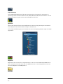
LayerProbe
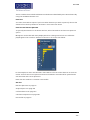
LayerProbe provides a non-destructive tool to measure the thickness and composition of surface and subsurface layers in thin-film structures. It integrates AZtec's robust quantitativeanalysis routines with a powerful thin-film analysis engine for reliable results.
n
Performs non-destructive analysis with minimal sample preparation
n
Predicts solvability and optimum experimental parameters to enable reliable, precise
measurements
n
Analyses layers down to 1nm thickness*
n
Handles total structure thickness up to several microns*
n
Includes a simulation tool to generate simulated X-ray spectra of thin-film structures
*Precise limits depend on the sample and can be determined using the Solvability Tool supplied with the software.
See LayerProbe on page 270
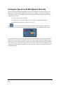
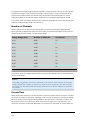
QuantLine (for SEM and TEM)
Quant LineScan determines elemental concentration variations across a user-defined line on
the sample.
n
Results can be viewed in either:
n
Schematic linescans for each element, or
n
A table showing the full quantitative data for each point (Wt% or At%). *
n
Points can be binned (by 2,4, 8, 16 and 32)*
n
Spectra can be extracted from any point on the linescan for further investigation*
* This functionality is also available for Line and TruLine.
See Acquiring linescans on page 391
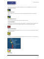
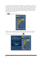
AutoPhaseMap (for SEM and TEM)
- ii -
What's New in AZtec 2.1
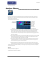
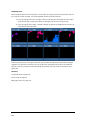
AutoPhaseMap is a new way to automatically create a map of the distribution of phases in a
sample automatically during or after acquisition:
n
Turns X-ray map data into Phase Map data in seconds.
n
Calculates and displays:
n
Distribution of each phase
n
Spectrum and composition for each phase
n
Area fraction for each phase
n
Finds phases and highlights elements that are present at only trace amounts.
n
Finds phases at all size ranges including nano-materials.
See Analyze Phases on page 375
EBSD
n
Reanalysis improvements
n
Live Monitoring
n
Phase fraction
n
Improvements in image acquisition for forescatter detectors
n
Drift correction using FSD images as references
n
Export Raw Unprocessed EBSPs for cross-correlation application
n
General performance and other EBSD improvements
Reanalysis improvements
The reanalysis functionality is now more versatile:
n
Multiple reanalysis of any map, so settings can be repeatedly optimised if required.
This includes changing the solver settings, and adding or removing phases.
n
If SmartMap EDS data is collected with an EBSD map, the X-ray data is now included
with that map when reanalysed.
n
EDS data is viewed and reported together with the EBSD reanalyzed maps.
n
Extract point EBSP and X-ray spectrum from any stored map data, including reanalyzed data.
See Reanalysis on page 465
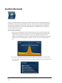
Live Monitoring
This feature monitors orientation information (EBSP, unit cell, pole figures) in real time to validate data quality.
During acquisition, the orientation information quadrant of ‘Construct Maps’ provides the following information:
- iii -
n
The EBSP, with optional overlay of the pattern centre and solution simulation,
n
The 3D unit cell and list of reflectors,
n
Selected pole figure with orientation of current pixel highlighted.
The refresh rate is selectable, up to 1 pattern per second. Acquisition speed is not affected.
If a solution is available, the name of the phase, number of bands, MAD and Euler angles from
the collecting point also display at the bottom of the orientation information quadrant.
Switch between monitoring live acquired patterns and stored patterns mode via a Toolbar.
The live unprocessed and processed pattern are also available in Mini View.
See Optimize Solver on page 444
Phase fraction
When collecting an EBSD map, the system now gives the % phase fraction of the phases
found:
n
Provides a real-time overview of the phases, and % phase fraction in the sample.
n
Avoids the need to export data to Channel 5 to see the phase fraction while collecting.
See Construct Maps on page 463.
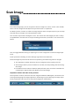
Improvements in image acquisition for forescatter detectors
Collect up to 6 individual FSD images simultaneously. The number of images collected
depends on the number of independent diodes on the detector. Functions include:
n
6-channel FSD images and a mixed FSD image are acquired and viewed in one interface.
n
Automatic optimization of each channel before scanning.
n
Offset and gain of each channel can be adjusted manually during image acquisition.
n
The weight of signal intensity for each channel in the mixed image is set to get the
best image.
n
Color may be selected for each channel image.
n
Optimization is possible on a reduced area – by selecting a reduced area map and
the optimization factor applied to the whole map. This is useful for images where
very dark regions (such as a hole) or very bright regions can distort the image optimization.
See Scan Image on page 418
Drift correction using FSD images as references
- iv -
What's New in AZtec 2.1
A new option allows the use of the FSD image as the tracking image to monitor and correct
for drift.
On a tilted sample, the FSD image often offers the best image for monitoring drift because it
can show more detail than the secondary electron image or backscattered electron image.
See AutoLock Settings on page 138
Export Raw Unprocessed EBSPs for cross-correlation applications
Raw 12-bit patterns as collected from the camera can be stored as TIFF files. These patterns
are not corrected for background, magnetic field, or lens distortion. These patterns are preferred for cross-correlation applications such as CrossCourt.
n
Unprocessed EBSPs are created during acquisition and collected in a folder with a
selected local destination.
n
Image format is uncompressed TIFF.
n
If required, the processed EBSPs can also be saved.
See Acquire Map Data - Settings on page 457
General performance and other EBSD improvements
n
Monitoring function for extract tool in Phase ID and Optimize Solver.
n
AutoID of the peaks in Spectrum Monitor, in Phase ID, and in the Mini View. Easy
identification of the elements in the sample.
n
The phase key in the phase map lists only those phases found in the map.
n
Some improvements to naming consistency, so that the name of EBSD Detail dialog
box is constant with the acquired map.
See Identify Phase on page 480, Optimize Solver on page 444, Acquire Map Data on page 450
and Construct Maps on page 463.
General improvements
n
Report Template Generator
n
Licensing improvements (AZtec and INCA)
n
Network Licensing (AZtec and INCA)
n
Interface modifications and GUI usability improvements
Report Template Generator
In addition to the comprehensive report templates available for reporting, a ‘Report Template Generator’ now allows the design of personalized report templates.
n
User interface is easy to use and intuitive
n
Word and Excel templates can be generated at the same time
n
Generate multiple-page templates
-v-
n
A4/Letter format
n
Portrait and landscape layouts
See Generating your own report template on page 51.
Licensing improvements (AZtec and INCA)
Extensive improvements have been made to the AZtec/INCA license activation/deactivation
process.
n
If a PC where you installed the software products does not have access to the internet, you need a unique unlock code from the internet-based licensing service to
enable you to use the software product. This long code needed to be manually copied and taken to a PC with internet access, where it had to be manually pasted.
n
There is now no need to manually copy and paste the long licence activation/deactivation codes from one PC to another.*
n
The Licence Manager automatically detects whether a USB stick is inserted in the
PC, and stores or loads any codes relevant to the current activation/deactivation
process.
n
The License Manager utility is also copied to the USB stick for use on internet PCs
without AZtec software installed.
n
An extensive user guide is included in the AZtec help
* Note: except when there is no internet access and no possibility to bring storage media to
and from the system PC
Network Licensing (AZtec and INCA)
An ‘AZtec Network licence’ is now available, which makes AZtec/INCA available to a large
number of offline PCs.
n
Network licences are designed for offline processing on multiple PCs.
n
Requires installation of the AZtec software on the individual PCs and on the user’s
local network server.
n
All installations on a single server need to be the same package (i.e. Standard,
Advanced, Automate)
n
Users on a PC connected to the local network server run the AZtec software locally,
and it automatically communicates with the server to see if any licences are available. If a license is available, the AZtec software runs as normal. If all licenses have
been checked out, the user receives a notification and has to contact the local
administrator.
n
The local administrator is notified when available licenses are running low.
n
The ‘Network license’ also allows users to ‘check-out’ an available license for use
away from the local server/network. This timed license deactivates when the period
has elapsed, and returns to the local server for re-use.
Note: CHANNEL5 still requires a HASP dongle.
- vi -
What's New in AZtec 2.1
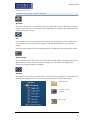
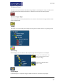
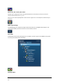
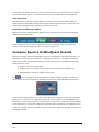
Interface modifications and GUI usability improvements)
n
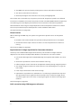
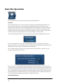
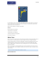
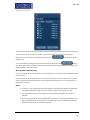
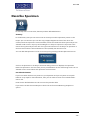
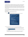
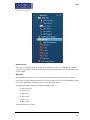
AZtec has a new welcome screen that allows:
n
Quick access to recent projects
n
Quick access to demonstration data for training purposes
n
Quick access to Help
n
Creation of a new project with an associated profile
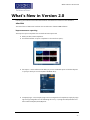
n
The Map and TruMap icons have been modified, and moved closer to the Start and
Stop buttons.
n
Choice of Weight% and Atomic% in the MiniQuant.
n
Map consistency: Users can now save not only map/colour selections directly to profiles from mapping navigator, but also the AutoLayer assignment so that the same
colours are used when going from area to area.
See Acquiring linescans on page 391, Construct Linescans on page 403, Acquire Map Data on
page 363, and Construct Maps on page 370.
- vii -
What's New in Aztec 2.0 SP1
SP1 contains mostly bug fixes, localization/help updates, some usability modifications and
one new functionality implementation.
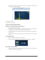
New functionality:
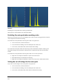
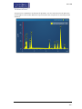
Users will now have the ability to hide the noise peak in their spectra via the right mouse button (this is a universal setting that once turned on applies to all spectra):
A selection of bugs that have been fixed in SP1:
- viii -
n
AZtec 2.0 stops working with LN2 detectors systems.
n
Irregular spectrum and mapping acquisitions were occasionally failing (when a user
draws a free hand acquisition area for spectrum acquisition of mapping, acquisition
would occasionally fail to start).
n
User defined energy windows in EDS mapping were not saving to profiles.
n
Wrong values of pre-tilted specimen holder were used during EBSD mapping
(under certain circumstances system uses tilt value from previous map).
n
Occasional connection errors to EBSD hardware.
What's New in Version 2.0
What's New in Version 2.0
Following are new features and enhancements included in this version of the software:
AZtecTEM
The main focus of AZtec 2.0 has been the introduction of AZtecTEM software.
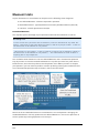
Improvements to reporting
The way the report templates are created has been improved:
n
Ability to edit/create templates.
n
Increased number of report templates to choose from (350+).
n
Site report – Users will have the ability to print a combined report of all data objects
in a project with just one click (EDS and EBSD data):
n
Company logo – The company logo can be changed for all templates, simply by copying the logo image file into the following directory - C:\Program Files\Oxford Instruments NanoAnalysis\AZtec\Reports.
- ix -
n
Annotations on spectra – annotations on spectra are now saved in the project and
will be visible on report templates:
See the link for details:
Report Results on page 44
General user interface enhancements
Software is now fully 64-bit, which means AZtec can:
n
Utilize more of the host PCs RAM.
n
Handle larger data sets (Software is now ideally placed to cope with the ever increasing demands for more and more data acquisition and storage).
n
Run multiple memory hungry Programs simultaneously without compromising the
performance.
n
Note: It is important to note that the software will now not run on 32-bit operating
system.
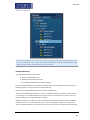
New navigator selectors
n
More robust user-friendly drop down selectors.
n
Future proof (easily copes with any new additions of techniques or navigators):
Batch export of data tree objects
n
-x-
Multiple data objects (images, spectra, IPF maps, etc...) can now be batch exported
as bmp, gif, jpeg, png, tiff or wmp files:
What's New in Version 2.0
n
Multiple data tree images can be saved at the original resolution, even if each image
has a different resolution:
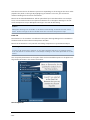
Settings panels
n
Settings panels can now behave in two different ways, depending on the users' preference:
n
Stay open until the cog or cross is pressed.
n
Stay open until a mouse click anywhere on the interface:
Interface reset
n
Once activated the interface layout will go back to default:
- xi -
kV visible on Mini View
EDS usability improvements and new functionality
n
Noise Peak - Option to Include/Exclude the noise peak in the scaling of the spectrum.
n
You can hide the noise peak if you do not wish to display it in the spectrum:
See the link below for details:
- xii -
What's New in Version 2.0
Context Menus - Spectrum Viewer on page 321
n
Pulse Pile Up overlay in ‘Confirm Elements’ step:
See the link below for details:
Confirm Elements - Settings on page 171
n
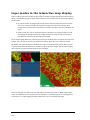
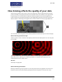
Pixel Binning available for Maps and Linescans – this not only improves the image
quality/statistics on an image with low counts, it also allows the large data sets to
be processed more easily.
n
n
No need to decide the pixel resolution when processing data:
Benefits of binning are illustrated in the screen shot below:
See the link for details below:
How binning affects the quality of your data on page 373
- xiii -
n
Compare step is now available in Guided Mode for ease of use.
n
Variable spectrum acquisition termination.
n
n
Now the users have the ability to set their own termination criteria:
Candidate element list is now collapsible:
EBSD usability improvements and new functionality
Solving Improvements
n
Developments in indexing algorithms. These changes make the indexing more
robust so that it is easier to get good quality data.
n
The EBSD indexing algorithm:
n
It is less sensitive to selection of number of bands.
n
It is easier to set up for data collection and to achieve a higher hit rate.
n
It is more effective at separating similar phases.
n
‘Band Width’ function replaced by ‘Grouping Function’ accessed
from the ‘Describe Specimen Step.
See the links below for detail:
Optimize Solver on page 444
Configuring groups of phases on page 417
Magnetic Field Correction for EBSP’s collected using SEMs with Immersion or ‘Semi-in
Lens’ objective lens
We now have the capability to correct EBSPs distorted by the magnetic field in the SEM
chamber, this method uses the model described in US Patent 2006 / 0219903.
n
- xiv -
This correction is designed to work on Hitachi and JEOL SEMs where the magnetic
field is typically required for high resolution imaging. Please check with OI to confirm that your instrument is supported.
What's New in Version 2.0
n
The solution requires collection of a distorted and undistorted pattern from the
same point, and then calculates a correction factor.
See the link below for detail:
Magnetic Field Correction Setup on page 440
Forescatter Detector Control Improvements
n
Additional functionality is included to aid the setting up and collection of FSD
images.
n
There are 2 default settings:
n
Atomic number contrast.
n
Orientation Contrast, as well as a customized setting.
See the link below for detail:
FSD Control Dialog on page 434
General Performance & Other EBSD Improvements
n
Faster Reanalysis.
n
Improved speed of the phase search in Phase ID.
n
CTF (Channel Text File) export.
n
TIFF export of EBSPs with both CPR and CTF format.
n
EBSD Reporting templates, for mapping and Phase ID.
n
EDS sum spectra can now be extracted from combined EDS/EBSD maps.
Top Tips Movie
A 'Top Tips' movie will be installed on to the PC desktop when version 2.0 software is
installed. (The directory: C:\Users\Public\Documents\Oxford Instruments NanoAnalysis\Documentation).
The movie reveals the lesser known but useful functionality in the software:
Training CD
A Training CD is now shipped with every system. The CD contains movies on the general operation of the software.
- xv -
Contents
Contents
0
Copyright
What's New in AZtec 2.1
What's New in Aztec 2.0 SP1
What's New in Version 2.0
Contents
Getting started
Application overview
i
ii
viii
ix
xvii
1
2
Navigators
5
Menu Bar
6
Preferences
13
Status Bar
20
User Profile
22
Support Panel
27
Report Results
44
Themes
53
Search Tool
54
Color key
55
FAQs about Software Licensing
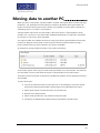
Moving data to another PC
56
59
Getting Help
61
EDS-SEM
63
Setup for EDS
65
Calibrate
66
Calibration Element
70
Calibrate for Beam Measurement- Settings
71
How to
EDS Qualitative Analysis
Analyzer - Guided
72
73
75
Describe Specimen
76
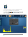
Acquire Spectra
96
- xvii -
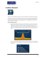
Confirm Elements
115
Calculate Composition
117
Compare Spectra
120
Analyzer - Custom
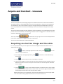
Acquire and Confirm
Point & ID - Guided
123
124
Scan Image
125
Acquire Spectra
146
Confirm Elements
170
Calculate Composition
185
Point & ID - Custom
199
Acquire and Confirm
201
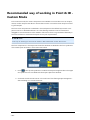
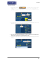
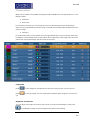
Recommended way of working in Point & ID - Custom Mode
202
Map - Guided
204
Acquire Map Data
205
Construct Maps
219
Analyze Phases
226
Map - Custom
Acquire and Construct
Linescan - Guided
236
237
239
Acquiring linescans
241
Displaying and manipulating linescans
243
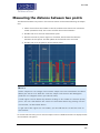
Measuring the distance between two points
245
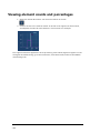
Viewing element counts and percentages
246
Comparing element quantities
247
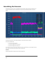
Smoothing the linescans
248
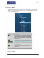
Linescan Data
249
Exporting the linescan data
250
Extracting a single spectrum from the linescan
251
Extracting multiple spectra from the linescan
252
Construct Linescans
255
Linescan - Custom
- xviii -
122
258
Contents
Acquire and Construct - Linescans
Optimize
Standardize
LayerProbe
LayerProbe
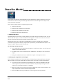
Describe Specimen
Describe Model
Scan Image
Acquire Spectra
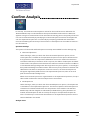
Confirm Analysis
Calculate Layers
Edit Materials
Simulate Spectra
Set Up Solver
LayerProbe Settings
EDS-TEM
Optimize
259
262
263
270
271
273
276
280
284
287
292
294
296
299
301
303
305
Calibrate
306
Calibration Element
308
Analyzer - Guided
309
Describe Specimen
310
Acquire Spectra
313
Confirm Elements
330
Calculate Composition
332
Compare Spectra
338
Analyzer - Custom
Acquire and Confirm
Point & ID - Guided
340
341
342
Describe Specimen
343
Scan Image
346
Acquire Spectra
350
Confirm Elements
353
Calculate Composition
355
Compare Spectra
358
Point & ID - Custom
360
- xix -
Acquire and Confirm
Map - Guided
362
Acquire Map Data
363
Construct Maps
370
How binning affects the quality of your data
373
Analyze Phases
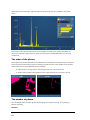
375
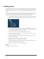
Finding phases
376
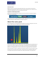
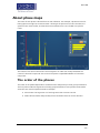
About phase maps
377
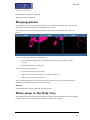
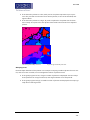
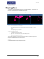
Merging phases
379
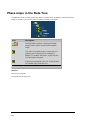
Phase maps in the Data Tree
380
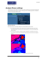
Analyze Phases settings
381
Analyze Phases toolbars
383
Map - Custom
Acquire and Construct
Linescan - Guided
386
387
389
Acquiring linescans
391
Displaying and manipulating linescans
393
Measuring the distance between two points
395
Viewing element counts and percentages
396
Comparing element quantities
397
Smoothing the linescans
398
Linescan Data
399
Exporting the linescan data
400
Extracting a single spectrum from the linescan
401
Extracting multiple spectra from the linescan
402
Construct Linescans
403
Linescan - Custom
Acquire and Construct - Linescans
EBSD
EBSD - Map
- xx -
361
406
407
411
412
Describe Specimen
413
Scan Image
418
Contents
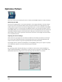
Optimize Pattern
436
Optimize Solver
444
Acquire Map Data
450
Construct Maps
463
Phase ID
473
Acquire Data
474
Search Phase
477
Identify Phase
480
Hardware Control
483
Detector Control
EBSD Detector Control
Microscope Control
Microscope Parameters
Index
484
489
493
496
499
- xxi -
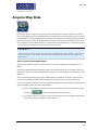
Getting started
Getting started
The unique features of the user interface are described in the Application overview followed
by the Guided tour of the Application. The details about the software licensing are covered in
the frequently asked questions:
Application overview
2
FAQs about Software Licensing
56
Moving data to another PC
59
-1-
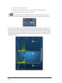
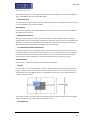
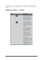
Application overview
There is a great deal of flexibility in the user interface. You can configure the workspace the
way you wish to work and save a custom configuration (layout) to come back to every time.
The main application consists of the workspace in the middle area. It is supported by a side
panel on the right containing Project Data, Mini View and Step Notes. You can remove each
of these components from the view if you wish.
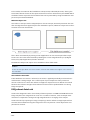
Dockable and Floating Window Panes
The window panes are docked as the default configuration of the user interface. You can undock and free float them. Click and drag them wherever you want them in the interface or to
a second monitor.
Re-sizable Windows and Dialogs
Windows and dialogs can be resized by clicking and dragging their edges. The main application window can also be re-sized.
Global Menu Bar
There is a Menu bar near the top of the application window. It has the common menu items
that you can access wherever you are in the application.
E
XAMP L E
Configurable Status Bar
The Status Bar is located at the bottom of the application window. You can choose which
hardware parameters you wish to display in there. A progress bar also shows up in the Status
bar when you are importing or saving a project.
Tool Bars
Various useful tools are available in local tool bars where appropriate.
E
XAMP L E
' P an ' , ' Normalize' , ' A n n otation s' , ' Sh ow Data Valu es' an d ' Sh ow Can didate
Elemen ts' tools are av ailable in a loc al tool bar in th e Con f irm Elemen ts an d in th e
-2-
Getting started
A c qu ire & Con f irm w in dow s in P oin t & ID on th e righ t of th e applic ation w in dow .
E
XAMP L E
Th is tool bar is av ailable in th e A c qu ire an d Con f irm w in dow in th e
Cu stom M ap n av igator. Y ou c an toggle on / of f th e u ser in terf ac e c ompon en ts f rom th e
display to y ou r pref erred lay ou t.
Context Menus
Many useful menu items are available on the right click of the mouse in the application.
E
XAMP L E
Image, Spec tru m an d M ap v iew ers h av e man y u sef u l men u items. For ex ample y ou c an
email a spec tru m, image or map or appen d it to y ou r report.
There are two modes of operation, Guided and Custom:
Guided Mode
The user interface components are laid out in Navigators that take you through your analysis
from the Specimen through to the Report. You can navigate backwards and forwards as you
wish. Each step has associated F1 (context sensitive) help and Step Notes to assist you at
each stage of your analysis.
Custom Mode
In this mode, the key components are provided in one window. It allows you to perform the
analysis in one workspace without having to move away from it. Each component can be
undocked to have it free floating or dragged to another monitor to view it in full screen.
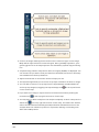
To provide you with more workspace, the Navigator area can be collapsed by pressing
in the top right of the application window. Press
to restore the Navigator.
Below are some key user interface elements which make the software unique:
Navigators
5
Menu Bar
6
Preferences
13
Status Bar
20
User Profile
22
Support Panel
27
Report Results
44
Themes
53
Search Tool
54
-3-
Color key
-4-
55
Getting started
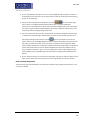
Navigators
The software has Navigators to guide the user through the analysis process. There are the following navigators in the software:
n
Analyzer - Guided on page 75
n
Analyzer - Custom on page 122
n
Point & ID - Guided on page 124
n
Point & ID - Custom on page 199
n
Optimize on page 262
n
Map - Guided on page 362
n
Map - Custom on page 386
n
Linescan - Guided on page 389
n
Linescan - Custom on page 406
n
EBSD - Map on page 412
n
Phase ID on page 473
-5-
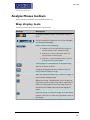
Menu Bar
There is a menu bar at the top of the application window containing several menu options.
Each menu has several items which are described below.
File on the facing page
View Menu on page 9
Technique selector on page 9
Tools Menu on page 10
Help on page 12
-6-
Getting started
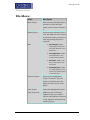
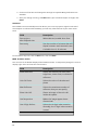
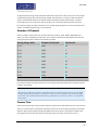
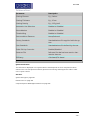
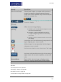
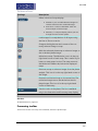
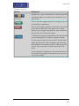
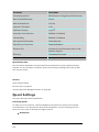
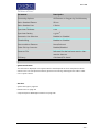
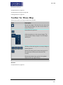
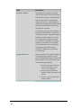
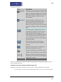
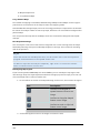
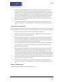
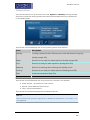
File Menu
Menu
Description
New Project
Removes any existing Projects,
prompts to save and then
opens a new Project as Project
1.
Open Project...
Removes any existing Projects
from the data tree, then opens
an existing Project, prompts to
save any existing Projects if
required.
Add
n
New Project: Adds a
new Project and leaves
any open Projects in the
data tree.
n
New Specimen: Adds a
new Specimen in the
Project that has focus.
n
New Site : Adds a new
Site in the Project that
has focus.
n
Existing Project...adds
an existing Project and
leaves any open Projects
in the data tree.
Remove Project
Removes the highlighted
Project. If there is only one
Project in the data tree, the
Remove Project menu is disabled.
Save Project
Saves the highlighted Project.
Save Project As...
Makes a copy of the highlighted Project, prompts to
enter a name and then opens it
in the data tree and closes the
existing Project.
-7-
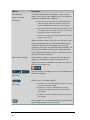
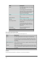
-8-
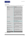
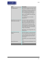
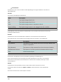
Menu
Description
Import INCA
Project...
Imports an INCA Project, adds
it to the Project list if existing
Projects contain data otherwise
replaces an existing “new
Project”.
Save As INCA
Project....
Saves the highlighted project
as an INCA Project.
Export to CHANNEL5 Project
Exports the currently selected
EBSD data as a CHANNEL5
project (CPR) file or a Channel
Text File (CTF). You may also
include EBSD patterns as
TIFF files. This option is not
available if you have stored
EBSPs without solving.
Recent Projects
Allows to load from the recent
Projects that you have been
working on.
Close
Shuts down the application.
Getting started
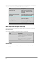
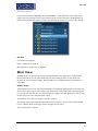
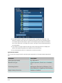
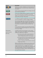
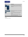
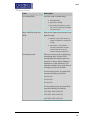
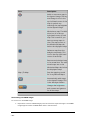
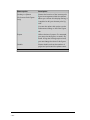
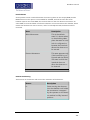
View Menu
Menu
Description
Data View
It has the Current Site and
Data Tree tabs.
Mini View
It has various views such
as a live spectrum, image
or acquisition progress
bar.
Step Notes
Provides a brief description of the main features
of each screen.
Users can write and edit
their standard operating
procedures (SOPs) for
future reference.
Application
Zoom Level
Available options are
Largest, Large, Medium,
Small and Smallest.
Reset Layout
Restores the default layout on restarting the
application.
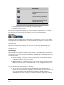
Technique selector
The techniques available are EDS and EBSD. Select the technique you wish to use by pressing
the appropriate selector button on the top left of the main screen.
-9-
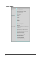
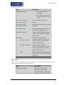
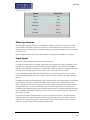
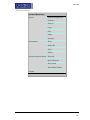
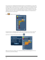
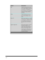
Tools Menu
Menu
Description
Themes
Accessible Theme
Oxford Instruments Theme
Light Blue Theme
Blue Theme
Languages
Default
English
French
German
Russian
Chinese Simplified
Japanese
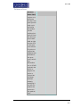
User Profile...
Settings available to create a user
profile are:
EDS Acquire Line Data Settings
EDS Acquire Map Data Settings
EDS Element Settings
EDS Peak Label Setting
EDS Quant Settings
Scan Image Settings
Specimen Tilt Settings
- 10 -
Getting started
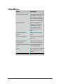
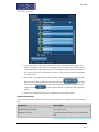
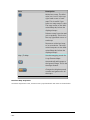
Menu
Description
Preferences...
Preferences are saved per user.
Make your selection for the following:
Auto Save
Image Viewer
INCA Image Export
Reports
Spectrum Viewer
Status Bar
Welcome Screen
Status Messages
- 11 -
Help Menu
Menu
Description
Show Help Home Page
Launches the Help Viewer
with table of contents in
the left pane and useful
links to internal and external sites in the right pane.
Show Step Help
Opens the Help Viewer.
Pressing F1 on the keyboard loads the help
page relevant to the
active step of the navigator.
Show NanoAnalysis
Advice
Opens links to 'How to'
topics.
Launch User Manual
Opens the user manual as
a PDF file.
Launch NanoAnalysis
Encyclopedia
Opens the Encyclopedia
in the Windows Explorer.
Oxford Instruments Web- Launches Oxford Instrusite
ments's home page.
About
- 12 -
Provides access to System
Info, Assembly Info and
Credits.
Getting started
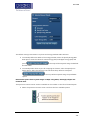
Preferences
You can change the appearance of many parts of the software to suit your own needs by
recording your preferences on the Preferences dialog. The software saves your preferences
on the computer that you are currently using. When you run the software again, it has the
appearance that you prefer. Your preferences will not be available if you run the software on
a different computer or with a different logon on the same computer.
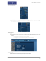
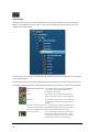
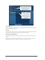
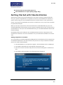
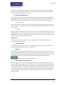
Setting your preferences
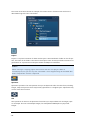
1. Click the Tools menu, then click Preferences to open the dialog.
- 13 -
2. Click one of the tabs and change the settings as required. Many preferences are
available.
3. After you change a setting, click Save. When you have finished your changes, click
Close.
Auto Save
The software can automatically save the data in your current project at regular intervals. If
the computer or software fails suddenly, you lose only a few minutes of your most recent
work.
Field
Description
Save project
after elapsed time
When selected, enable Auto Save.
Save every
Sets the number of minutes that will
elapse between each automatic save.
A suitable time is 10 minutes.
To save data at any time, click the File menu, then click Save.
EBSD 3D Phase Viewer
You can control the default display of the 3D Phase viewer. To temporarily change the current
display, right-click it and use the context menu.
- 14 -
Field
Description
Show reflectors
Shows the reflectors as solid lines,
edge lines, center lines, or shows no
reflectors.
Unit Cell Color
Selects the color of the selected
phase.
Max Reflectors
Selects the maximum number of
reflectors that you can specify.
Show Unit Cell
Shows an image of the unit cell
inside the sphere.
Use Perspective
Makes the image appear threedimensional.
Use 4 Digit Indices
Selects the 4-digit index notation.
Generally, the 3-digit index notation
is used.
Getting started
EBSD Image Viewer
You can control the default display of the Electron Backscatter Diffraction (EBSD) image. To
temporarily change the current display, right-click it and use the context menu.
Field
Description
Band Mode
Shows the bands as edges or center
lines.
Sum Indices
Shows only those indexes where the
sum of the indices does not exceed
the number you enter here. For example, if the value entered is three,
indices such as 100 and 111 may be
labeled, if displayed, on the simulation. However indices whose sum
is greater than 3 will not be shown.
The value entered must be between
1 and 20.
Min Intensity
Determines how many bands are
shown in the simulation. A value of 0
shows all bands. A value of 15 shows
only those bands with an intensity
greater than 15. The value must be
between 0 and 100.
Extend Bands
Shows the bands extended beyond
the band detection area.
Use 4 Digit Indices
Selects the 4-digit index notation.
Generally, the 3-digit index notation
is used.
Display Simulation
Shows a simulation of the solution as
an overlay on the EBSP.
Display Band Detection
Area
Shows the band detection area as a
circle.
Display Bands
Shows the Kikuchi bands.
Display Pattern Center
Shows the pattern center as a green
cross.
EBSD Pole Figure Viewer
- 15 -
You can control the default display of pole figures and inverse pole figures. To temporarily
change the current display, right-click it and use the context menu.
Field
Description
Projection Type
Offers a choice of the type of
projection - equal area or stereographic.
Overlay Inverse Pole Figure
on Sphere
Shows the location of the inverse
pole figure within the sphere.
Show Great Circles
Shows the latitude and longitude
lines on the sphere.
Use 4 Digit Indices
Selects the 4-digit index notation. Generally, the 3-digit index
notation is used.
EDS Layered Image Settings
You can control the default display of the layered image to include new X-ray map layers.
EDS Linescan Viewer
You can select the default line thickness (in pixels) for the linescans.
Field
Description
Default Line Thickness Offers a thickness from Thin (0.5 pixels)
to Thicker (4.0 pixels). The default line
thickness is Thick.
For any other thickness , select User
defined, and move the slider bar.
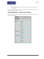
Spectrum Viewer
You can control the default display of the Spectrum Viewer. To temporarily change the current display, right-click it and use the context menu.
- 16 -
Getting started
Field
Description
Vertical Scale Type
n
Linear shows a regular
spaced grid.
n
Logarithmic is useful for displaying data that has a wide
range.
Show Horizontal Scale
Show Vertical Scale
Shows the scales of keV and
cps/eV.
Lock Vertical Scale
Lock Horizontal Scale
Prevents the Pan tool from moving
the graph.
Smooth Spectrum
Shows a smooth representation of
the normally spiky spectrum.
Expand Mini Quant
Shows the expanded Mini Quant
display in the top right corner of
the spectrum.
Noise Peak:
Shows the noise peak, and
includes its value if you reset the
scales (using the context menu
option "Reset Scales").
n
Include in Scaling
n
Exclude from Scaling
Shows the noise peak, but
excludes its value if you reset the
scales (using the context menu
option "Reset Scales").
n
Hide
Hides the noise peak. Specify the
energy level in the "Cutoff Energy
(keV)" box. .
Image Viewer
You can control the default display of the Image Viewer. To temporarily change the current
display, right-click it and use the context menu.
Field
Description
Rescale Image Mode
Changes the scale of the
image. For a large image,
select Fill Display with Image.
- 17 -
Field
Description
Show Acquisition Areas
Offers a choice of display for
the acquisition areas.
Show Short Names
Shortens the labels for the
acquisition areas to prevent
them from overlapping and
masking the text.
Show Header
Shows the label for the image
in the header.
Show Color Bar
Shows the Color Bar below the
Image Viewer. You can move
the slider on the Color Bar to
change the contrast of the
image.
Show Scale Bar
Shows a micron marker below
the Image Viewer.
Show Contrast/Brightness Buttons
Shows the Auto and Manual
buttons at the bottom right
corner of the image.
Show Annotations
Shows any annotations on the
image.
Show Color Key
Shows a color key of the
phases in the bottom left part
of the Layer Image in the Map
application.
Use Image Smoothing
Smoothes the lines in the
image. If this check box is not
selected, the image might
appear more pixilated.
INCA Image Export
If you save your project as an INCA project, you can export a Secondary Electron (SE) or Backscattered electron (BSE) image.
Reports
You can select the layout, scale and content of your reports. A report is typically a Microsoft®
Word document or a Microsoft® Excel spreadsheet. If you do not have those software applications installed, you can still view and print the reports with the Microsoft® viewers that are
- 18 -
Getting started
supplied with the software. To edit the reports, you need Microsoft® Office 2007 (or later)
software installed on your computer.
Field
Description
Report Image Scaling (Pix- Sets the image scaling.
els Per Inch)
The default is 96 pixels per inch,
which is suitable for displaying on a
computer screen. For high-quality
printing, select a higher number.
Show Acquisition Areas in
Reports
Offers a choice to show any acquisition areas.
By default, reports show none.
Package Templates
Offers a choice of templates for each
package. A report is a Microsoft®
document or spreadsheet in one of
several page sizes. Letter is popular
in the USA.
The default paper size, A4 is popular
in Europe.
Other Templates
Offers a choice of templates for the
batch export of data.
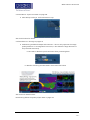
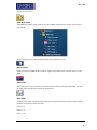
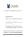
Status Bar
You can select the parameters (such as microscope voltage and noise levels) for EDS and
EBSD that will appear in the Status Bar at the bottom of the software window.
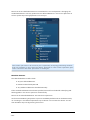
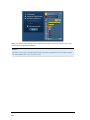
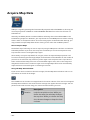
Welcome Screen
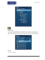
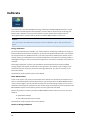
You can choose whether the Welcome Screen appears when you start the software. The Welcome screen shows a list from which you can quickly select any of your recent projects.
See also
Status Bar
- 19 -
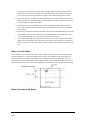
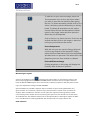
Status Bar
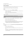
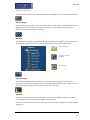
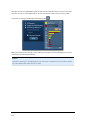
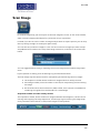
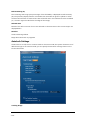
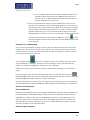
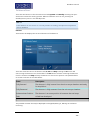
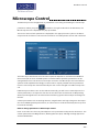
The Status Bar displays the hardware status. It also allows the access to the Microscope Control, EDS detector and EBSD detector. A progress bar appears in the Status bar when you
import, load or save projects.
The user selected parameters are displayed in the Status Bar at the bottom of main application screen. You can choose the parameters you wish to display on the Status Bar tab in
the Preferences dialog. To access the Preferences dialog go to the Tools menu on the main
tool bar and select Preferences:
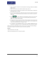
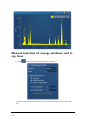
Check the relevant check boxes to make your selection and press the Save button. The
selected parameters will be displayed in the Status Bar.
You can access the Microscope Control by pressing
Status Bar.
- 20 -
located on the right end of the
Getting started
See Also:
Microscope control on page 493
Microscope Parameters on page 496
- 21 -
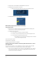
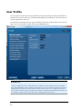
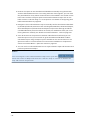
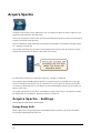
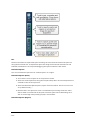
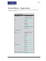
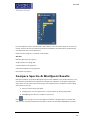
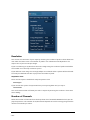
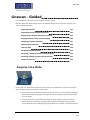
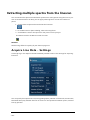
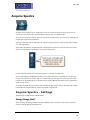
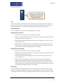
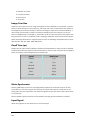
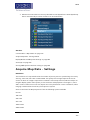
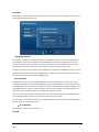
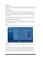
User Profile
A user ‘Profile’ contains all the settings needed to reproduce analytical results obtained on a
previous date or by another user. The User Profile dialog is launched from the Tools menu on
the main application menu bar.
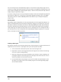
To show only the settings for your type of analysis, select from the drop-down list in the top
right corner. For example, change All Settings to EBSD Settings.
E
XAMP L E
“ I am in c h arge of a serv ic e lab an d h av e a n u mber of u sers reportin g to me. We perf orm man y dif f eren t ty pes of an aly sis th at w e c arry ou t, bu t do n ot h av e th e lu x u ry of
assign in g on e person to do th e same an aly sis all th e time. So it is importan t th at w e
h av e a w ay of redu c in g th e v ariability in an aly tic al resu lts betw een dif f eren t u sers. A t
th e momen t I make su re I c h ec k th e u sers' settin gs bef ore th ey start ”
- 22 -
Getting started
For each analysis type, all the relevant parameters can be saved in a profile, along with personalized step notes to instruct the users on the analysis. Subsequently anytime a user
wishes to perform a particular type of analysis, all they have to do is load the relevant profile
and all the appropriate settings will be changed and associated step notes will be loaded.
E XAMP L E
“ M y c ompan y h as sev eral sites all ov er th e w orld, perf ormin g similar ty pes of an aly sis.
We n eed to en su re th at eac h site c arries ou t th e same ty pe of an aly sis in th e same
w ay , so w e c an c ompare resu lts” … … … . “ I n eed some h elp in terpretin g rec en tly
ac qu ired data… . if I sen d a projec t to Ox f ord In stru men ts Cu stomer Su pport, h ow do I
en su re th at th ey see w h at I do?”
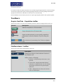
For both these cases the user profile can be exported via the user profile window:
The profile will be saved as a .config file and there will be user standards file (with .ois extension) if selected for use. See Managing Standardizations on page 267
- 23 -
Both files must be given to the person who you want to repeat or look at your data. The recipient will have to go to the Load Profile window and import the supplied profile.
E
XAMP L E
For spec tru m ac qu isition , y ou c an spec if y th e Nu mber of Ch an n els, En ergy Ran ge
( keV) , P roc ess Time, A c qu isition M ode an d A c qu isition Time ( s) an d sav e th em in th e
User P rof ile.
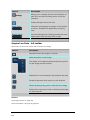
When the User Profile dialog is opened, it stores the backup copy of the current settings.
Press
in the User Profile dialog to load a profile.
Press
in the User Profile dialog to save a profile.
Press
in the User Profile dialog to save the settings. This action will close the
dialog and remove the backup copy.
Press
backup copy.
to close the dialog. This action will restore the current settings from the
There are separate tabs for different settings in the User Profile dialog. The details of the settings in each tab are described in the topics which can be accessed from the links below.
See Also:
Scan Image - Settings on page 421
Acquire Line Data - Settings on page 252
Acquire Map Data - Settings on page 211
Acquire Spectra - Settings on page 313
Element Settings below
Peak Labels on page 158
Quant Settings on page 187
LayerProbe Settings on page 301
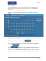
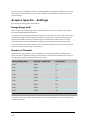
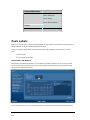
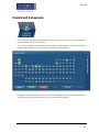
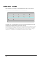
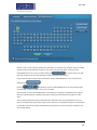
EDS Element Settings
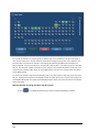
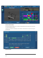
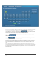
The Element Settings tab in the User Profile dialog is provided with a periodic table. It enables
you to define a list of Pre-defined Elements present in the specimen and the elements you
wish to exclude from the AutoID routine.
When you press an element symbol in the periodic table, three buttons are enabled which
are colored coded:
Include
Exclude
- 24 -
Getting started
Clear
Defining an element from the periodic table is a cyclical process. Double-clicking on an element symbol will include this element. It will be colored green. Double-clicking it again will
exclude this from the list and it will be colored red. Double-clicking on the symbol third time
will clear this element from the list.
TIP!
For multiple element selection, hold down the Ctrl key, press on each element in the
periodic table that you wish to select and then press the Include, Exclude or Clear button.
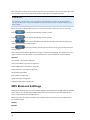
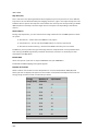
AutoID Settings
You can enable or disable AutoID during acquisition by checking or un-checking the 'Perform
AutoID during acquisition' checkbox.
AutoID Confidence Factor
The default value for the Confidence Factor is set at 3. You can use the slider to set the value.
The Confidence Factor is used to determine how AutoID behaves with regard to the sources
of error.
Map Element Details
The 'Map Element Details' dialog allows you to configure the element maps. The default X-ray
lines are used for element mapping unless you specify them. You can select the X-ray line for
each element that you wish to map from the Map Element Details in the Element Settings tab
or in the Construct Maps step.
You can define the energy window width for each element rather than using the default
value.
You can select which elements to map and which ones to exclude.
See Also:
Auto ID Confidence Factor below
Auto ID Confidence Factor
If the Confidence Factor is set to a high value, AutoID will find the most significant peaks but
may miss small peaks that are close to the noise level. If the Confidence Factor is set to a low
value, AutoID will detect small peaks but may pick up false positive identifications that are
due to statistics or systematic errors.
By default, we set the Confidence Factor to 3 which corresponds to the "3-sigma" confidence
level for a normal statistical error distribution.
The Confidence Factor is used to determine how AutoID behaves with regard to the sources
of error. AutoID is designed to find a good combination of peak profiles that matches the
spectrum and thus identifies the elements present in the specimen. When peaks overlap, the
- 25 -
proportion of constituent profiles is determined by least squares fitting to the sum of peak
profiles. Counting statistics introduce fluctuations into the spectrum that are sometimes difficult to distinguish from genuine peaks. The statistical fluctuations introduce "random"
errors that are equally likely to be positive or negative. When there are severe peak overlaps,
it is even more difficult to distinguish genuine peaks from noise fluctuations.
In addition, chemical bonding effects and inaccuracies in peak profiles may mean that there is
no combination of peak profiles that is an exact match to the spectrum, even when there is
no statistical noise. If the peak profile is not perfect, this introduces bias or "systematic" error
into the results.
If a fitted peak profile is much larger than the random or systematic errors, it is likely that the
corresponding element is present in the specimen.
N ote
To acces s t h e A u t oI D Con fiden ce F act or , s elect Us er Pr ofile fr om t h e Tools
men u an d t h en s elect t h e Elemen t Set t in gs t ab. A u t oI D Con fiden ce F act or
is available in t h e A u t oI D Set t in gs .
- 26 -
Getting started
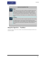
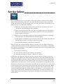
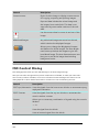
Support Panel
The Support Panel is present on the right side of the application window. It has three components, Data View, Mini View and Step Notes. You can add or remove any of these components from the display by selecting the View menu on the Menu bar. You can also
minimize, maximize or close each component from the display by pressing the relevant button present at the top right corner of each component.
To increase your work area you may wish to collapse the Support Panel by pressing the arrow
button in the top right corner of the application. Pressing this again will restore the Support
Panel.
Data View
Data View has two tabs, one for the Current Site and one for the Data Tree. For details see
the Data View topic from the link at the end of this topic.
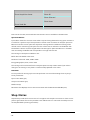
Mini View
In the Mini View you can choose to display a number of different views such as Electron
Image, Spectrum Monitor, the Ratemeter or many others depending on the step.
Step Notes
Step Notes provides the first time user of a navigator with simple instructions on how to complete a typical work flow. It also provides a site administrator or user with the ability to write a
standard operating procedure (SOP).
See Also:
Mini View on page 93
Step Notes on page 94
- 27 -
Data View
The Data View panel is located on the right of the main application window, By default, it is
always displayed. If it has been taken off the view, it can be restored by choosing the Data
View from the View menu on the main menu bar.
Data is archived in a logical manner and can be directly viewed via easily recognizable icons.
Acquired data is automatically saved at the end of an acquisition. An auto save option can be
enabled from the Auto Save tab of the Preferences on page 13 dialog on the Tools menu.
The Data View panel has two tabs, Current Site and Data Tree.
See Also:
Current Site on the facing page
Data Tree on page 85
- 28 -
Getting started
Current Site
The Current Site shows the data for the currently selected Site in the Data Tree, plus the current acquisition and any pending acquisitions. The ordering of items in the Current Site is different to the Data Tree. The new data items are added to the end in the Current Site where as
the Data Tree sorts the items under the Site by spectra, electron images and then maps.
The Current Site has some extra features:
Electron Image
Electron image has a lock/unlock icon. Click once to lock, then again to unlock:
If unlocked, subsequent electron image acquisitions in the same Site will replace the existing
electron image.
Locking the Electron Image will prevent the image from being recycled.
Current Acquisition
Both Spectrum and Map acquisitions show a progress bar and a stop icon:
When acquiring EBSD data, pause/resume and restart icons are also shown. Progress information is also shown in the tool tip.
Pending Acquisitions
Spectrum shows a cancel icon:
Note spectra and map acquisitions can be queued.
See Also:
Data Tree on page 85
Data Tree Menus on page 38
- 29 -
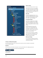
Data Tree
Data is archived in a logical manner and can be directly viewed via easily recognizable icons on
the Data Tree. To access the Data Tree, select the Data Tree tab on the Data View panel.
All open Projects and their contents are displayed in the Data Tree. Multiple Projects can be
opened and shown in the Data Tree at the same time. If you have multiple Projects, Specimens or Multiple Sites in the Data Tree, you can easily get to your current site by pressing
the Current Site tab.
When the application is started a default Project containing a Specimen and a Site is shown.
As you acquire data, items are added to the Data Tree. The current items in the Data Tree are
shown in bold.
Clic k on an item on th e Data Tree to make it c u rren t.
Items on the Data Tree
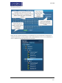
The screen shot below shows an example of the main items in the Data Tree. Each item is
described along with their icons below:
Project
Project is a top level container for data. Each Project is associated with a folder on the file system. The name of the folder is the same as the Project name. The Project folder contains a single file with an .oip extension and optional Data and Reports sub folders.
N ote
Wh en mov in g or c opy in g projec t data en su re th at th e root projec t f older is
mov ed/ c opied, n ot ju st th e . oip f ile. Th e f older c an be zipped u sin g th e stan dard
- 30 -
Getting started
Win dow s c ompression u tilities if requ ired.
Specimen
Specimen represents the real specimen that you analyze and collect the data from, including
images, maps and spectra. There may be many Specimens in a single Project. A Specimen may
contain more than one Site.
Site
Site represents an area on the Specimen from where you acquire data such as images, spectra and maps. Site can hold multiple images, for example SE and BSE plus any imported
images.
The analytical conditions such as kV, Magnification and Calibration are stored with the data.
Electron Image
Electron Image on each Site can be a secondary electron (SE) image, a backscattered electron
(BSE) image, or a forward-scattered electron image. You can acquire two images simultaneously if suitable hardware is available.
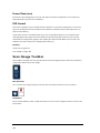
FSD Data
This folder is the container for all FSD data. It contains electron images from each diode, and
the FSD mixed image, which is the result of combining some or all of the FSE images.
Folder of images
Image from a single
FSD diode
Mixed image
- 31 -
Imported Image
Any standard Windows Picture files can be imported into the Project for comparison or
reporting. The file formats available are JPG, JPEG, BMP, PNG, WDP, GIF, TIF and TIFF. You can
import an image using the context menu available from the Site.
Spectrum
Spectra are acquired from the areas defined on an electron image. Sum Spectra and Reconstructed Spectra are shown under the Map in the Data Tree.
You will see the following items in the Data Tree if you are acquiring element maps in the EDS
application:
Map Data
Map Data is the container for a mapped area(s) in a Site. It can hold EDS Data, EBSD Data or
both. One Site can contain more than one Map Data items. In the example above there are
two items, Map Data 1 and Map Data 2.
EDS Data
- 32 -
Getting started
EDS Data is the container for Map Sum Spectrum, Reconstructed Spectra, X-ray element
maps, and Phase Images.
Map Sum Spectrum
The sum spectrum is calculated from the data acquired from all the pixels in the electron
image.
Reconstructed Spectrum
You can reconstruct spectra from regions of maps or linescans.
X-ray Element Maps
The data can be processed as Windows Integral Maps or TruMaps (FLS maps). The Data Tree
is populated with the appropriate maps on selection of the map processing option:
Windows Integral Maps
The standard element maps obtained from the counts in the element energy window including the background.
TruMap
The maps are corrected for peak overlaps and any false variations due to X-ray background.
Phase Image
- 33 -
Phase Image is the container for all the phase maps and their spectra. For example:
An image of an individual phase. The
name is composed of its elements,
for example: AlMgO.
A spectrum extracted from all the
points in a phase.
Layered Image
Layered Image is a composite image created from electron and X-ray map images.
Linescan Data
The data tree contains a Line item under the Site; this is the container for the line data. By
default, this is labeled as ‘Line #’ where # is an auto-increasing number under the current
site(Site 1) as shown below:
The Line item is the container for EDS Data. All linescans and the sum spectrum are contained
within the EDS Data.
- 34 -
Getting started
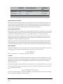
The Linescans can be processed as Windows Integral Linescans, TruLines or QuantLines. The
Data Tree is populated with the appropriate Linescans on selection of the processing option:
Windows Integral Lines- The standard element linescans obtained from
the counts in the element energy windows
can
including the background.
TruLine
The Linescans are corrected for peak overlaps
and any false variations due to X-ray background.
QuantLine
The linescans are processed to show relative percentages of each element by weight or number
of atoms.
The label of the element linescan is composed of the element symbol followed
by the lines series used for TruLine/Window Integral data analysis. For example
Cr Kα1 is the label for a Chromium Linescan obtained from the Kα1 line.
Line Sum Spectrum
The sum spectrum is called Line Sum Spectrum.
The region the spectrum comes from is visible
on the electron image. This is the same region
as where the linescan data is acquired from.
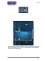
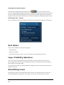
EBSD Data Folder
The EBSD Data folder is the container for the six Map components as shown in the screen
shot below:
These components are described briefly with their respective icons:
Band Contrast
Band Contrast is an EBSP quality number, higher the number more contrast there is in the
EBSP.
- 35 -
Phase Color
This component colors the pixels in the map based on which phase was identified. The color
for each phase is defined in 'Phases for Acquisition'.
Euler Color
The Map component colors the map based on the Euler color scheme and will help to show
different orientations within the map.
Euler 1= R
Euler 2= G
Euler 3= B
IPF X Color, IPF Y Color, IPF Z Color
The IPF color components color the pixels based on the orientation of the unit cell and
chosen reference direction; x, y or z.
Note that the color key depends on the structure type so it is not always the easiest map to
interpret.
EBSD Layered Image
A Layered Image is a composite image created from electron and EBSD map images or element maps if EDS is present as shown in the screenshot above.
Point Data
In Phase ID, a Point Data node appears in the Data tree when spectra and EBSP are acquired
from the points defined on the image:
- 36 -
Getting started
Reanalyze Data
If you have acquired an EBSD Map with stored EBSPs it is also possible to reanalyze a map
region with new settings such as new solver settings or even solving by including different
phases. Re analyzed map data is stored in the data tree as shown in the screen shot below:
See Also:
Current Site on page 29
- 37 -
Data Tree Menus below
Moving data to another PC on page 59
Data Tree Menus
Each item such as Project, Specimen and Site in the Data Tree has its own menu items. Right
click with the mouse on a particular item to access the menu entries.
The menu entries for each item on the Data Tree are described below:
Project
There are two menu items for the Project, Remove and Edit Notes.
n
Remove - removes the project from the Data Tree. This option is disabled if only one
Project is in the Data Tree.
n
Edit Notes - opens a dialog for editing Project notes.
n
Details - opens a dialog showing the Project label and Date/time when the Project
was created.
TIP!
To rename a Project select Save Project As... from the File menu.
Specimen
There are four menu items for the Specimen, Rename, Delete, Edit Notes and Details.
n
Rename - allows to rename a Specimen.
n
Delete - deletes the Specimen from the Project.
n
Edit notes - opens a dialog for editing Specimen notes.
n
Details - Opens a dialog showing the Specimen Label, Specimen Orientation and Pretilted Specimen Holder. The Details dialog will also include the specimen coating
information if you have selected it in the Describe Specimen step.
Site
There are six menu items for the Site, Rename, Delete, Import Image, Batch Report, Print
and , Email
- 38 -
n
Rename - allows to rename a Site.
n
Delete - deletes the Site from the Project.
n
Import Image - imports any standard Windows picture file for comparison or reporting.
n
Batch Report - this saves the Microsoft® Word or Excel report of all the data in the
Site. It uses the report Batch Template selected in the Preferences dialog accessed
from the Tools menu.
Getting started
n
Print - this prints the Microsoft® Word or Excel report of the data associated with
the Site.
n
Email - this helps to send the report via Email.
Electron Image
The menu items are:
n
Rename - renames the Electron Image.
n
Delete - deletes the Electron Image.
n
Add to Layered Image - adds an electron image to the current Layered Image.
n
Add to Image Viewer- adds an electron image to the current FSD Mixed Image.
n
Save As - Saves the current electron image in Microsoft® Word or Excel report.
n
Print - prints the current electron image in Microsoft® Word or Excel report.
n
Email - sends the image via Email.
n
Details - opens the dialog showing the image details.
N ote
Y ou c an v iew reports w ith th e M ic rosof t® Word/ Ex c el v iew ers su pplied w ith y ou r sy stem. H ow ev er, M ic rosof t® Of f ic e n eed to be in stalled f or editin g y ou r reports.
Spectrum
There are six menu items for each spectrum on the Data Tree, Rename,Delete, Save As,
Print, Email and Details.
n
Rename- this renames the spectrum.
n
Delete - this deletes each spectrum.
n
Save As - saves the current spectrum in a user selected picture file format.
n
Print - prints the current spectrum as an image.
n
Email - sends the spectrum via Email.
n
Details - opens the dialog showing the spectrum details.
N ote
H old Ct r l an d c lic k on items on e by on e on th e Data Tree f or mu lti - selec t / de- selec t.
H old S hif t an d c lic k on c h ildren on e by on e in a bran c h on th e Data Tree f or mu ltiselec t/ de- selec t.
Map
There are six menu items for Map on the Data Tree, Rename, Delete, Save As, Print, Email
and Details.
n
Rename - this renames the current map.
n
Delete - this deletes the current map.
- 39 -
n
Save As - saves the current map in a user selected picture file format.
n
Print - prints the current map.
n
Email - sends the current map via Email.
n
Print - prints the current spectrum as an image.
n
Details - opens the dialog showing the map details.
Layered Image
There are six menu items for the Layer Image, Rename, Delete, Save As, Print, Email and
Details:
n
Rename - this renames the Layered Image.
n
Delete - this deletes the Layered Image.
n
Save As - saves the current Layered Image in Microsoft® Word or Excel report.
n
Print - prints the current Layered Image in Microsoft® Word or Excel report.
n
Email - sends the Layered Image via Email.
n
Details - opens the dialog showing the Layered Image details.
EDS Data
There are two menu entries for the EDS Data, Rename and Delete
n
Rename - this renames the EDS Data.
n
Delete - this deletes the EDS Data.
X-ray Map
There are six menu items for each X-ray Map, Rename, Delete, Save As, Print, Email and
Details:
n
Rename - this renames the X-ray Map.
n
Delete - this deletes the X-ray Map.
n
Save As - saves the current X-ray map in Microsoft® Word or Excel report.
n
Print - prints the current X-ray map in Microsoft® Word or Excel report.
n
Email - sends the map via Email.
n
Details - opens the dialog showing the Layered Image details.
EBSD Data
There are four menu items for EBSD Data, Rename, Delete, Export... and Details...
- 40 -
n
Rename - this renames the EBSD Data.
n
Delete - this deletes the EBSD Data.
n
Export - exports the currently selected EBSD data as a CHANNEL5 project (CPR) file
or a Channel Text File (CTF). You may also include EBSPs as TIFF files. This option is
not available if you have stored EBSPs without solving.
n
Details - opens the dialog showing EBSD Data Details.
Getting started
Each map components (Band Contrast, Phase Color, Eulor Color, IPF X, IPF Y and IPF Z) has six
menu items:
n
Rename - this renames the selected component.
n
Delete - this deletes the selected component.
n
Save As - this saves the selected component as an image file.
n
Print - prints the selected component.
n
Email - sends the selected components via email.
n
Details - opens the dialog showing details of the selected component.
Point Data
There are two menu items for the Point Data , Rename and Delete.
EBSD Point n
There are six menu items for each EBSD Point as in the case of each map component
described earlier.
Spectrum n
There are six menu items for each Spectrum as in the case of each map component.
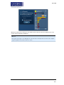
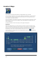
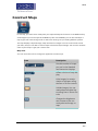
Mini View
The Mini View is an area of the Support Panel dedicated to the display of a number of different views which you can select depending on what data you wish to view. Views containing the current Electron Image , Spectrum Monitor or EDS Ratemeter are examples of
such views.
Electron Image
The full field of view of the currently selected electron image is displayed here. It is often useful to refer to this image in steps where your application area is dedicated to displaying spectra or maps. For example you can view the electron image in the Mini View if you wish to view
full size spectrum in the Acquire Spectra step.
The features of the electron image in the Mini View are:
The default state is full image with Scale Bar (micron marker). You can remove the Scale Bar
from the display by de-selecting it from the image context menu.
The Context menu items are:
Show Acquisition Areas
Show All
Show Selected
Show None
- 41 -
Show Scale Bar
Features such as Pan, Zoom and User Annotations are not available in the Mini View.
Spectrum Monitor
It provide a means for the user to see what X-rays are being detected at any given moment. It
is useful for a quick survey of the specimen to find an area of interest for analysis. Spectrum
Monitor uses the current spectrum acquisition settings with the additional setting of the
refresh rate for monitoring the spectrum. This refresh time is referred to as the Buffer Size.
The default is 20 but can be changed under the Settings for Spectrum Monitor in the Miniview. Increasing the Buffer Size corresponds to a longer refresh rate.
The settings in the Spectrum Monitor are:
Buffer Size: The default value is 20.
Number of Channels: 1024, 2048 or 4096
Energy Range (keV): 0-10, 0-20 or 0-40
The settings can be selected from the Acquire Spectrum step or Mini View. If you make a
change in the setting in one place it is automatically updated in the other.
Ratemeter
It is very useful for setting up the microscope beam current while viewing the X-ray acquisition parameters:
Input Count Rate (cps)
Output Count Rate (cps)
Dead Time (%)
Ratemeter also displays the current Process Time and the Recommended WD (mm).
Step Notes
Step Notes provide the first time user of a navigator with simple instructions on how to complete a typical work flow. It also provides a site administrator or user with the ability to write
an SOP (Standard operating procedure).
A default editable set of notes are provided for each navigator step. The user can then overwrite these or add notes as required. A reset to default settings is available.
The notes are saved with the current user profile.
See Also:
Step Notes Editor on the facing page
- 42 -
Getting started
Step Notes Editor
The editor allows you to format text as you would using a word processor. You can cut, paste
and copy text, left, right and central align the text, change the font size and style, undo and
redo, select bulleted list or numbered list and paste in a picture.
- 43 -
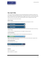
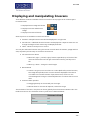
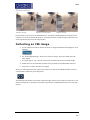
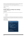
Report Results
You can quickly and easily generate reports from the data in your project. Each navigator has
a default report template. A report is generated from this template when you click the Report
Results button on the main navigation bar.
Once the report is generated, the software automatically displays the new report so you can
view, edit or print it.
You can change the default report template by selecting it from the Report Preferences or
accessing the Report Templates from the down arrow on the Report Results button.
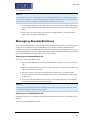
Managing your reports
You can click the down arrow on the Report Results button to open a menu of options that
enable you to manage your reports. Some options are available only if Microsoft® Word or
Excel is installed. In some cases, the appearance of the Report Results button changes to indicate the last action that you performed, so for example, you can send reports by email in
quick succession
The following menu options affect individual reports:
Menu
option
(Information
at the top of
the menu)
Appearance of the
Report Results
icon
Description
Shows the name of the report template
that is selected by default for the current navigator.
If no name is shown, select Report Templates, choose from a template from
the list, and click Set As Default.
Save As
- 44 -
Asks for a file name, then saves the
report as a Microsoft® Word or Excel
file. The default location for your new
report is in the Reports sub-directory of
your current project.
Getting started
Menu
option
Appearance of the
Report Results
icon
Append
(if Microsoft® Word
or Excel is
installed)
Description
Appends your report to the open file if
a report is already open.
Asks for a file name if no report is open.
Print
Generates a report and prints it immediately on your default printer. As an
alternative, you can use Save As, and
print the document later.
Email
Sends the report using the default
email package installed on your computer.
The following menu options affect site reports and report templates:
Menu option
Description
Site Report
Generates a report about every type of
information taken from the site. You
can choose the format (Word or Excel),
paper size, and file location.
(if Microsoft® Word or Excel is
installed)
Report Templates
Shows a list of the available templates.
See the next section about the Report
Templates dialog.
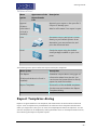
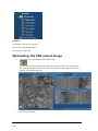
Report Templates dialog
Reports are generated from the templates, which determine the look and feel of the final
report. A set of templates are provided with the software. These templates include items
which you might like to save, print or email, for example Quant Results and Spectra. You can
view the complete set of templates by clicking the down arrow on the Report Results button,
then selecting the ‘Report Templates’ option:
- 45 -
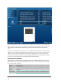
If Microsoft® Word or Excel is installed on your computer, the lower part of the dialog shows
a preview of your report. You can click on the title of any report in the list above it to see different layouts. To change the magnification, right click the preview and use the context
menu.
Note that the preview works only if your version of Microsoft® Word can save a document as
XPS format. Office 2010 is supported, but Office 2003 is not. For Office 2007, see the File menu
option, 'Save as’. If your Office 2007 does not have the XPS option, you can copy a ‘plug-in’
from the product DVD (in folder, Customer Support\Office2007). Alternatively, you can download from: http://www.microsoft.com/download/en/details.aspx?id=7
Filtering the list of templates
Initially, the list on the top right of the dialog shows all the available templates. To find a suitable template quickly, use the drop-down lists in the top left of the dialog to filter the long
list and show fewer templates.
Menu
Description
Document
Type
Shows only the templates that are in Microsoft® Word or Excel
format.
Orientation
Shows only the templates that have portrait or landscape layout.
- 46 -
Getting started
Menu
Description
Paper Size
Shows only the templates that are suitable for printing on a
paper size of Letter or A4. Letter is popular in the USA. A4 is
popular in Europe.
Directory
Shows templates from all directories or only one directory.
n
"System" shows the templates as supplied with the software.
Unless more templates are created, you see templates only
this directory.
n
"Current User" shows your own templates.
n
"All Users" shows templates you share with other users on
the same computer, and possibly on the same network.
Category
Shows only the templates that are suitable for images, maps or
spectra.
Technique
Shows only the templates that are suitable for EDS or
EBSD analysis.
Show Favorites Only
Shows only your favorite report templates. To mark a favorite,
click the star in the column to the left of the title.
If extra templates have been created for you and other users, you might see more templates
if you do not select System from the Directory drop-down list:
n
"Current User" shows your own templates. They are available only when you logon
to your user account.
n
"All Users" shows templates you share with other users on the same computer, and
possibly on the same network (depending on the network configuration).
Using the dialog buttons
The buttons around the dialog allow you to print or email the report, for example.
Button
Description
Updates the list of templates here if you have added a new template, or changed a template design, or changed some configuration information.
Opens a dialog where you can generate your own report template.
- 47 -
Button
Description
Save As
Asks for a file name, then saves the selected report as a Microsoft® Word or Excel file. Alternatively, you can double-click a
template in the list. The default location for your new report is in
the Reports sub-directory of your current project.
Append
Appends your selected report to the open file if a report file is
already open.
Print
Generates a report and prints it immediately on your default
printer. As an alternative, you can use Save As, and print the document later.
Email
Sends the report using the default email package installed on
your computer.
Set As
Default
Sets the selected template as your preferred default report template for the current navigator. For example, you can change the
current template to Excel format instead of Microsoft® Word
format.
You can also change the default report template from the Tools
menu by changing it in the Report Preferences.
Report Preferences
The preferences used for generating reports are accessed via the Tools menu on the main
application screen. Select Preferences and then select the Reports tab. Preferences allow you
to specify how your images will look in your final reports and which Report Template is associated with each navigator.
The following dialog shows a typical choice of report templates. Your list of reports might be
different because of the products that are installed.
- 48 -
Getting started
The resolution of images in your reports can be specified by setting the Dots per Inch (DPI)
option. You can specify whether the area selections are shown in the Electron Images.
The Report Preferences also allow you to specify which Report Template is associated with
Batch Reporting mode. This is useful for generating similar reports for many sites.
Generating similar reports for many sites
The software has a Batch reporting feature which allows you to generate similar reports from
any number of sites. For example you can generate a report containing only electron images
and spectra from every site.
Decide which report template to use for generating your batch report. You need to do this
only once. For example, you want reports of spectra always to be Word documents for printing later in Letter size:
- 49 -
1. On the Tools menu, select Preferences, and then select the Reports tab.
2. On the Reports tab under Batch Report, select a suitable template, for example:
Image & Spectra - Letter.docx.
To generate a Batch report at any time:
1. On the Data Tree, select one or more sites, then right click, and select Batch Report.
2. Select a folder for your reports, and click Select Folder .
One document is generated for each site. The documents are named according to the project
name, the site name, and the current date and time.
Compile a report on the fly
You can prepare your report as you acquire data.The image, spectrum and map viewers have
a range of context menus which allow you to export live or stored data. You can copy images,
spectra or maps to the clipboard and paste them into Microsoft® Word or Excel. You can
manipulate images, spectra and maps using various settings such as width, height, aspect
ratio and zoom before exporting to a third party reporting application. You can email or print
an image, spectrum or map from the respective viewer.
See Also
Context Menu - Report Templates below
Preferences on page 13
Changing the logo in your reports on the facing page
Generating your own report template on the facing page
Context Menu - Report Templates
After you select a template for a report, you can change the magnification of the preview in
the lower part of the dialog. Right click on the preview to see the following menu:
Menu option
Description
Increase Zoom
Increases or decreases the magnification of the preview.
Decrease Zoom
Alternatively, you can hold down the
Control key and move the mouse wheel
to zoom in and out. Fit to Height
- 50 -
Adjusts the magnification of the preview so that a single page fits within the
full area of the window.
Getting started
Menu option
Description
Fit to Width
Adjusts the magnification of the preview so that the page fits the full width
of the window.
Changing the logo in your reports
A standard report typically contains a logo, usually at the foot of the first page. If you prefer
to use your own logo, you can replace the supplied logo. To make this change, you must have
an administrator password.
1. In the folder where you installed the software (usually C:\Program Files), find the file
logo.png in a subfolder called Reports.
2. Open the file in a suitable graphic editor, such as Microsoft® Paint.
3. Record the size of the original logo, for example, width x height= 150 x 75. (In Microsoft® Paint, this information is in Properties.)
4. In another folder, create your own logo.
n
If your logo is smaller than the original logo, surround your logo with
white space to increase the image size.
n
If your logo is larger, surround it with white space to increase the image
size, and then crop the white space to create an image that has the same
aspect ratio as the original image , for example 400 x 200.
5. Name your logo file as logo.png, and copy it into the installation folder. You might
be prompted for an administrator password.
All subsequent reports will display your new logo. If the Report Template dialog is currently
open, and your new logo does not appear immediately, click Refresh List and wait a few seconds.
Generating your own report template
Although the software includes a comprehensive list of report templates, you might sometimes need to create a new report template. The Report Template Generator allows you to
design a new report template and publish it for personal use or to be shared with other
users. You can use the new template straightaway for producing Microsoft Word and Excel
reports. You can also save the template in an intermediate form, which allows you to continue to update the template design over time.
To create a report template:
- 51 -
1. In the Report Templates dialog, click the Template Generator button:
2. In the Report Template Generator dialog, enter a title for your template.
3. To ensure that you can easily find your template later, specify its properties by selecting the technique, category, paper size, and orientation.
4. Under Components, select the information that will appear in your report. For example, to add the date, go to General and click Date, which has this icon to denote it as
a piece of text:
An area appears on the white page.
5. Move your cursor onto the page, then move or stretch the area, as required. You
can also delete any unwanted component. For a context menu, right-click the area.
6. Repeat the previous steps to select further components and complete your template.
7. To add an extra page, click the “Add New Page” button, which is in the bottom right
corner:
8. To generate the templates, click Generate (in the menu bar). In the “Template Generation Options” dialog, enter the details. If you will be the only user of this template, select "Current User". You can create Word and Excel templates.
9. Click OK to create the report templates. You cannot change the design of these
report templates.
10. If you intend to change the design of your template later, click File > Save or File >
Save As to create an intermediate (XML) file at a convenient location.
11. Click OK to close the dialog.
12. To close the Report Template Generator dialog, click “X” in the top right corner.
13. To quickly find your new report template, look in your list of favorites.
Changing an existing report template
If you saved your previous design as an intermediate (XML) file earlier, you can open the file
again, and continue working on your template design.
1. In the Report Templates dialog, click the Template Generator button:
2. In the Report Template Generator dialog, click File > Load.
3. Using the file browser, locate the intermediate (XML) file, and click Open.
4. Continue working on your design.
- 52 -
Getting started
Themes
There are different themes i.e., color schemes available to choose to display the User Interface
for example:
Accessible Theme
Light Blue Theme
Blue Theme
- 53 -
Search Tool
Enter one or more keywords in the Search Help field near the top right corner of the application window or Help Home Viewer and press
. The Help Viewer is displayed with links
to a list of topics containing the keywords. When you click a topic link, the topic is displayed
in the Help Viewer. You can go back to the list of topics by pressing the back arrow near the
top left corner of the Help Viewer.
The keywords are highlighted in each topic . To remove all search highlighting, click this icon
in the toolbar above:
- 54 -
Getting started
Color key
The color key is an optional feature on many images. This key (or legend) explains the colors.
For more information, hover the cursor over each colored square. For example:
To show or hide the color key:
1. On the image, right-click to open the context menu.
2. Select View, then Color Key.
- 55 -
FAQs about Software Licensing
How can I activate my License Code?
You will need Internet access to Activate your License Codes. If the software is installed on a
computer with Internet access you can simply enter the License Code into the License Manager and press the Activate button. The Licence Manager will then automatically send your
License Code number to the remote licence server and, provided your License Code is valid,
an Unlock Code number will be returned to the Licence Manager that will unlock the software you have purchased. Once Activated you will not need to do this again unless you want
to Deactivate a License Code. Each software platform has its own separate License Code so
you will need to do this for each platform.
My system computer does not have Internet access so how can I activate my
License Code?
If your system does not have direct access to the Internet you can still Activate your License
Code using any other computer with Internet access.
See NLS Getting Started Card and User Guide for details.
Can I install the software on more than one computer (PC or Laptop) at a time?
Yes you can. The terms of the license allow you to install the software on any number of PCs
within your organization, but you will only be able to use the software on computers which
have a valid License Code installed and Activated.
What is a single license?
Unless you specifically ordered multiple licenses when you purchased your system, you will
have a single licence which means you can Activate your software only on one computer at a
time. (If you need to run the software on more computers you can Deactivate one computer
and Activate another or you can buy additional licenses.)
What is a multiple license?
If you purchased multiple licenses you will be able to run the software on the corresponding
number of computers at the same time. For example, if you purchased five licenses you can
Activate the software on a maximum of five computers, then if you try Activating a sixth computer you will be advised that all of your licenses are in use. Unless you specifically ordered
multiple licenses when you purchased your system, you will have a single licence which means
your software can only be Activated on one computer at a time. (If you need to run the software on more computers you can of course Deactivate one computer and Activate another
or buy additional licenses.)
I ordered multiple licenses so why have I only got one License Code?
The License Code contains details of the software you have purchased and are entitled to use
and the number of licenses (computers) you are entitled to Activate at the same time. So if
you purchased five licenses you will only receive one License Code but it will allow you to Activate five computers at the same time using the same License Code.
- 56 -
Getting started
What is a License Code?
A License Code is a unique 18-digit number which you will have received with your system. It
contains encrypted details of the software you have purchased including the modules (functionality) and the number of licenses. When this number is entered into the software Licence
Manager and the code is Activated the software functionality you purchased and are entitled
to use is unlocked.
Can I use my single software on a different PC or Laptop?
Yes, you can. If you have your software installed on another computer you will need to Deactivate the license on the existing computer, and then Activate the license on the other computer. Transferring the Active license to the second PC does of course mean that your
software will no longer run on the first (Deactivated) computer (because you only have a single license). Each software platform has its own separate License Code so you will need to do
this for each platform.
Can I transfer my (single) license between computers more than once?
Yes, you can transfer (Deactivate and Activate) a license any number of times, but remember
you can only Activate a single license on one computer at a time.
Can I use my software on more than one PC or Laptop at the same time?
Although you can install your software on more than one computer at the same time, if you
have a single license you can only activate it on one of them at a time. If you have a multiple
licenses you can activate the license on as many computers as your license allows. If you want
to use your software on more computer than you currently have licenses for you can easily
buy additional licenses as required from your representative.
I have forgotten the password. What can I do??
If you cannot remember a password when re-activating a license, you can request a new password to be sent to the email address that was given during registration.
This feature is available only if the mail server has been configured correctly.
Tip: Alternatively, you can register the license code with a new user name and password.
To set up the mail server:
1. On the licensing server, open the License Manager. For details, see section 1.4.
2. Select the “Settings” tab.
3. Enter the fully qualified domain name of the mail server, for example: mail.example.com.
4. Click Save.
To request the new password:
1. On the registration page, click the “Forgotten password” link.
2. Follow the instructions on-screen.
- 57 -
How do I upgrade my license?
If you are upgrading your license, you need to deactivate and reactivate the license to pick up
the new modules. For details, see the sections in the Software Licensing User Guide. You will
need to know the user name and password that was set at the time of registration.
If you forget the password, you can recover it by an email method. You need to know the
email address that was registered with the user name. If you do not know the user name and
password, you can activate the software product by registering with a new user name and
password. You will need the license code.
N ote
Y ou c an ac c ess th e L ic en se M an ager f rom Tools in Ox f ord In stru men ts Nan oA n aly sis
grou p of programs.
- 58 -
Getting started
Moving data to another PC
When you start a new Project, a Project folder is created. The Project folder contains a Project
file with an ‘.oip’ (Oxford Instruments Project) extension. By default the Project folder and
Project file use the same project name, however it is possible to rename either of these provided the project is not open in the software.
A Project folder may contain two sub folders, ‘data’ and ‘reports’. Acquired data is either
stored in the ‘.oip’ file or in the ‘data’ folder if additional data files are required. It is possible
for a Project to not have a ‘data’ sub folder.
The ‘reports’ folder is the default location for saving any reports generated from the Project
by the user. Reports can be saved in other locations where necessary. Before moving a
project, please close any reports saved in the ‘reports’ subfolder.
An example of a project folder is shown in the screen shot below:
To move the project, either copy or move the Project folder to it’s new location. This will maintain the folder structure, and allow the project to be opened from it’s new location.
The Project can be opened on a second PC provided the software and an appropriate license
are installed.
To open the Project:
n
Launch the software either from the shortcut on the desktop or from the Oxford
Instruments NanoAnalysis folder in All Programs on the Windows Start menu.
n
Select Open Project from the File menu on the menu bar.
n
Browse to the Project folder.
n
Select the Project file with .oip extension and press Open.
n
The Project is loaded and the data items are populated in the Data Tree.
- 59 -
Getting Help
Getting Help
Various elements of Help available in the software are described below:
l
Context Sensitive Help (F1)
The active workspace in the application has an associated help topic. Press F1 to
access the help topic. Each help topic has useful links for further information.
l
Step Notes
A default editable set of notes are provided for each navigator step. The user can
then overwrite these or add notes as required. A reset to default settings is available.
l
On-Line Help
There are six options available from the Help menu on the application menu bar:
A. Show Help (F1)
This opens the Help Viewer with TOC in the left pane and the help topic on the
right. You can also launch the Help Home Page by pressing
in the top right
corner of the application window. The Home Page has the facility for searching the
Help by entering the key words in the search field. It has links to the following four
help items:
n
Getting Started
This opens a page with links to topics to give you information about the main features of the user interface and Frequently asked questions about the software
licensing.
n
Oxford Instruments Website
This opens the Oxford Instruments Website.
n
Support
- 61 -
This links to Oxford Instruments Support Website.
n
NanoAnalysis Encyclopedia
This opens the Encyclopedia that contains help topics with interactive diagrams
and movies. It provides the background information, theory and instrumentation
of Microanalysis techniques.
l
Show Nano Analysis Advice
It has a number of topics which provide step by step advice on most frequently
performed tasks.
l
Launch User Manual
This opens the User Manual in PDF format. The manual is supplied with a table
of content and a comprehensive Index.
l
Launch Nano Analysis Encyclopedia
This is another way of launching the Encyclopedia.
E. Visit Oxford Instruments Website
This launches Oxford Instruments website.
l
About
The About dialog opens. It has Software version number and Copyright statement.
You can access License information, System information, Assembly information and
Credits.
l
Search Help
The Search Help field is near the top right corner of the application window.
To find a single word or any combination of words, type each keyword here. To find
a specific phrase, include double quote marks around the keywords. Then press:
The Help Viewer is displayed with links to a list of topics containing the keywords or
the phrase. When you click a topic link, the topic is displayed in the Help Viewer. You
can go back through the list of topics by pressing the back arrow near the top left
corner of the Help Viewer:
- 62 -
EDS-SEM
EDS-SEM
Setup for EDS
65
Calibrate
66
Calibration Element
70
Calibrate for Beam Measurement- Settings
71
How to
72
EDS Qualitative Analysis
Analyzer - Guided
73
75
Describe Specimen
76
Acquire Spectra
96
Confirm Elements
115
Calculate Composition
117
Compare Spectra
120
Analyzer - Custom
Acquire and Confirm
Point & ID - Guided
122
123
124
Scan Image
125
Acquire Spectra
146
Confirm Elements
170
Calculate Composition
185
Point & ID - Custom
199
Acquire and Confirm
201
Recommended way of working in Point & ID - Custom
Mode
202
Map - Guided
204
Acquire Map Data
205
Construct Maps
219
Analyze Phases
226
Map - Custom
236
Acquire and Construct
Linescan - Guided
237
239
- 63 -
Acquiring linescans
241
Displaying and manipulating linescans
243
Measuring the distance between two points
245
Viewing element counts and percentages
246
Comparing element quantities
247
Smoothing the linescans
248
Linescan Data
249
Exporting the linescan data
250
Extracting a single spectrum from the linescan
251
Extracting multiple spectra from the linescan
252
Construct Linescans
255
Linescan - Custom
Acquire and Construct - Linescans
Optimize
259
262
Standardize
- 64 -
258
263
EDS-SEM
Setup for EDS
There are two calibration routines available in the Calibrate step of Optimize navigator,
Energy Calibration and Beam Measurement. To ensure that you understand when to calibrate your system and which calibration routine to use, read the comprehensive details
below:
Calibrate
66
Calibration Element
70
Calibrate for Beam Measurement- Settings
71
- 65 -
Calibrate
Two calibration routines available are Energy Calibration and Beam Measurement. For qualitative and normalized quantitative analyses, you will need to perform only the Energy Calibration part. However, if you are interested in accurate quantitative analysis with unnormalized results, you will need to perform the Beam Measurement routine too.
N ote
Y ou c an ac c ess th e Calibration rou tin es f rom th e Calibrate step in th e Optimize n av igator.
Energy Calibration
For accurate identification of peaks, you need to perform the Energy Calibration. Energy Calibration measures the shift in the position of the spectral peaks and resolution of the system.
As the system has very stable electronics, you may only need to calibrate the system once in
several months, provided the environmental temperature of the laboratory is fairly stable. A
few degrees change in the environmental temperature can cause a small shift in the position
of peaks.
The Energy Calibration routine is performed for representative Process times, available
energy ranges and number of channels in one operation. This means if you change any of
these settings soon after you perform the Energy Calibration, you will not need to re-calibrate the system.
See details on how to perform the routine below.
Beam Measurement
If you are an expert user, and you need more than relative concentrations and require accurate un-normalized quantitative analysis results, you must perform the Beam Measurement
routine. Any change in the microscope settings such as accelerating voltage or lens control
will lead to the change in the beam current. Under these circumstances you must perform the
Beam Measurement routine before you do accurate quantitative analysis.
Note that you do not need to perform the Beam Measurement routine if you are only interested in:
n
Qualitative Analysis
n
Normalized Quantitative Analysis
See details on how to perform the routine below.
Details on Energy Calibration
- 66 -
EDS-SEM
Why do we need to perform Energy Calibration?
n
Ambient temperature changes will alter the gain of the system and this will affect
where peaks appear in the spectrum. The exact peak positions and the resolution
of the system are needed to precisely identify individual peak components in the
spectrum.
n
If peaks overlap, the relative sizes of individual peaks can only be calculated accurately if the width and position of each peak is accurately known. By measuring the
position of one known peak, the system can be optimized to determine the position
of all other peaks.
How often should I perform Energy Calibration?
The electronics used is carefully designed to provide good temperature stability. Since a
change of 10°C produces only a 1 eV shift in peak position, most routine analysis can be performed without re-optimizing peak position. However, if you need the software to resolve
very closely overlapped peaks, you should perform Energy Calibration and re -optimize if the
ambient temperature changes by a few degrees. With a good laboratory temperature control
you may not need to optimize for many months.
How to perform Energy Calibration
Energy Calibration requires the acquisition of a high quality spectrum from a suitable element
from which details of the spectrometer gain are calculated and stored. One element can be
used for both the Energy Calibration and Beam Measurement or you can use two different
elements if you wish.
You can use an element as an energy calibration standard as long as the calibration peak is
not overlapped by other peaks. There should not be any peaks within 100 eV of the calibration peak.
To perform Energy Calibration follow the steps:
n
Select Energy Calibration from the Calibration Routine drop-down list.
n
Select an element from the Calibration Element drop-down list.
n
Get the element standard in the field of view of the microscope. Adjust the working
distance to the recommended value and the beam current to achieve an optimum
count rate.
- 67 -
n
Press
to start acquisition of the calibration spectrum. The current settings will be used to acquire the spectrum. A window will be painted across the
peaks of the element X-ray line series.
n
A progress bar near the top of the Calibrate window displays the estimated time for
the completion of calibration spectrum acquisition.
n
On completion of spectrum acquisition, a message is displayed asking you if you
wish to perform the Energy Calibration. Press Yes if you wish to perform the Energy
Calibration.
Note that the details of the Energy Calibration can be found in the Spectrum Details dialog in
the Calculate Composition step when a spectrum has been quantified.
Details on Beam Measurement
For Beam Measurement, you must use a pure element standard and it must be stable under
the beam. See Calibration Element.
Note that the acquisition settings chosen in the Acquire Spectra step are carried across to
the Optimize Navigator and vice versa. Changing the settings in one will automatically
change the settings in the other.
Why do we need to perform Beam Measurement?
n
The microscope beam current may vary with time. If we want to measure absolute
concentrations, we need to make a comparison of intensity of a peak with that from
a known material. If we measure a known material, we can then make accurate
intensity measurements on unknowns, provided the beam current doesn’t alter
after the optimization.
How often should I perform Beam Measurement?
n
If you wish to calculate un-normalized totals, the frequency with which you perform
the optimization will depend on the stability of the beam current. Repeated measurement of a known standard will indicate whether the beam current is varying. The
variation in the analysis total will be in direct proportion to the change in current
since the last optimization.
How to perform Beam Measurement
The Beam Measurement routine requires the acquisition of a high quality spectrum from a
suitable element from which details of the beam current is calculated and stored. One element can be used for both the Beam Measurement and Energy Calibration or you can use
two different elements if you wish.
To perform Beam Measurement follow the steps:
- 68 -
EDS-SEM
n
Select a calibration routine from the drop-down list of Energy Calibration and Beam
Measurement.
n
Select an element from the Calibration Element drop-down list.
n
Choose the spectrum acquisition parameters from the Settings cog. For details see
Beam Measurement- Settings.
n
Get the element standard in the field of view of the microscope. Adjust the working
distance to the recommended value and the beam current to achieve an optimum
count rate.
n
Press
to start acquisition of the calibration spectrum. The current settings will be used to acquire the spectrum. A window will be painted across the
peaks of the element X-ray line series.
n
A progress bar near the top of the Calibrate window displays the estimated time for
the completion of Beam Measurement routine. The progress is also displayed in the
Current Site tab of Data View in the Support Panel.
n
On completion of the Beam Measurement routine, a message is displayed to save it
if you wish. If you decide to save it, the calibration spectrum is saved in your Project.
Note that the details of Beam Measurement can be found in the Spectrum Details dialog in
the Calculate Composition step when a spectrum has been quantified.
See also:
Calibration Element on next page
Calibrate for Beam Measurement- Settings on page 71
- 69 -
Calibration Element
Select the element that you wish to use for calibration from the drop down list. The choice of
element depends on whether you are doing Energy Calibration or Beam Measurement.
For Energy Calibration
The elements available for Energy Calibration are tabulated below:
Si
P
S
Cl
Ar
K
Ca
Sc
Ti
V
Cr
Mn
Fe
Co
Ni
Cu
Zn
X-ray peaks often involve multiple lines and in order to achieve accurate calibration, a large
peak with well-known line energies and intensities is required.
Therefore, for this reason we recommend that for energy calibration a pure element is used.
If a pure element is not available compounds that have K lines that are not overlapped may
be used instead. However, there may be some loss of accuracy because the line energy in a
compound can sometimes be up to 2eV different from that in the pure element.
For Beam Measurement
The system standards were calibrated using Co as the beam measurement element. Pure Co
resists oxidation and polishes well and is therefore the most suitable choice to monitor beam
current when you want to obtain accurate un-normalized or "absolute" estimates of composition. However, below 15kV, Co K is weakly excited and it is preferable to choose another
pure element for monitoring. The system will then make suitable corrections to allow the following pure elements to be used:
Si
Ti
V
Cr
Mn
Fe
Co
Ni
Cu
Zn
If the beam measurement standard is oxidized, contaminated or has a rough surface, then
this will have a direct effect on analysis totals.
- 70 -
EDS-SEM
Calibrate for Beam Measurement- Settings
When you select Beam Measurement, the Settings icon is enabled. These are the same X-ray
acquisition parameters which you have selected in the Acquire Spectra step. You can change
the settings here if you wish. The parameters selected in the Optimize navigator will be used
when you start acquiring spectra from your specimen.
Energy Range (keV)
The appropriate energy range should be selected in conjunction with the current microscope
accelerating voltage. If the accelerating voltage is above 10 kV, in order to view lines which
may be excited above 10 keV, the 20 keV range should be chosen. Below 10 kV, it may be
more appropriate to choose the 10 keV range since no lines above 10 keV will be excited.
In the Auto mode, the system checks for the accelerating voltage selected on the microscope
and sets a suitable energy range in the software.
Number of Channels
Select the number of channels from the drop down list of 1024, 2048 and 4096 with which you
display the spectrum. The number of eV/channel will depend on both the energy range and
the number of channels you select.
In the Auto mode, the system checks for the energy range selected and sets the appropriate
number of channels.
Process Time
Select the Process Time from the drop-down list of 1 to 6. The Process time is the length of
time spent reducing noise from the X-ray signal coming from the ED detector during processing. By selecting different Process times it is possible to reduce differing amounts of noise.
The longer the Process Time, the lower the noise. If noise is minimized, the resolution of the
peak displayed in the spectrum is improved, in other words, the peak is narrower and it
becomes easier to separate or resolve, from another peak that may be close by in energy.
If Default is selected, the Process Time is automatically set to a suitable value. There is a trade
off between the Process time that is used, and the speed at which data can be acquired into
the X-ray spectrum.
Total counts in spectrum
The default value for 'Total number of counts in spectrum' is displayed here. This value is used
to acquire a spectrum before the Beam Calibration is performed. You can enter the value that
you wish to use.
The default value for the total number of counts is 600,000. It is the total number of counts in
a Co spectrum acquired at 20 kV. It gives an approximate precision of 1% in the value of beam
current over a spread of ±0.5%.
See Also:
Acquire Spectra - Settings on page 313
- 71 -
How to
In this section users are provided step by step advice on the most frequently performed
tasks. The following tasks are described in details:
EDS Qualitative Analysis
- 72 -
73
EDS-SEM
EDS Qualitative Analysis
In EDS, the qualitative analysis is the process of identifying elements present in a specimen. It
involves acquiring a spectrum from the specimen and then identifying the peaks in the spectrum. Peaks can be manually identified to confirm elements using sophisticated tools available in the software. Once you have identified all the elements you can produce a Microsoft®
Word or Excel report. You can email the spectrum to your customer directly from the spectrum viewer provided your system is connected to the network and it has appropriate software installed.
You can use the confirmed elements list for elemental maps and quantitative analysis.
Below is step by step guide for qualitative analysis to get the most accurate results out of
your system with minimal effort:
n
If you know what elements are present in your specimen and you only want to see
peak labels or X-ray maps or X-ray linescans for those elements, then you can select
them in the Pre-defined Elements tab in the Describe Specimen step of Point & ID,
Map or Linescan navigator.
n
If you are interested in seeing what other elements might be present, then select
the AutoID option by checking the 'Perform AutoID During Acquisition' check box.
N ote
Ch ec k th e EDS Elemen t Settin gs in th e User P rof ile dialog ( av ailable f rom th e Tools
men u ) to en su re th at th e elemen ts th at y ou h av e pre- def in ed in th e Desc ribe Spec imen step are n ot in th e Ex c lu sion Elemen ts L ist. Users c an h av e dif f eren t ex c lu sion
lists.
n
Acquire an electron image from an area on your specimen in the Scan Image step
available in the Point & ID, Map and Linescan navigators.
n
Navigate to the Acquire Spectra step. Press
to acquire a spectrum
from the entire image. If you wish to acquire a spectrum from a point or an area on
the image, select the appropriate tool from the toolbar on the left side of the
screen. For details see How to acquire spectra on page 148
n
For details of spectrum manipulation and annotation see Acquire Spectra - Toolbar
on page 151
n
You can see your MiniQuant results in a table or a bar chart during analysis. Real
time Compare and instant MiniQuant options are available in the Acquire Spectra,
Confirm Elements and Calculate Composition (Comparison of Results - Two Spectra
template) steps. You can compare your current spectrum to a control spectrum during acquisition. For further details see Compare Spectra & MiniQuant Results on
page 195
- 73 -
n
Peaks in the spectrum are identified and labeled automatically using the AutoID
and Pre-defined elements lists. If too many peaks are close together, you can move
the peak labels for clarity. Select the Annotation tool available in the toolbar on the
left of user interface in Acquire Spectra and Confirm Elements steps. Click on the
label to select it and then drag it to a new position. For details of configuring peak
labels see Peak Labels on page 158
n
Navigate to the Confirm Elements step to manually confirm the elements identified
by AutoID (if selected). Extensive tools including Show Markers, Show Peak Shapes,
Show Fitted Spectrum, Show Theoretical Spectrum (from the Settings) and Show
Candidate Elements (from the toolbar on the left) are available to assist you in confirming elements manually. For details see Confirm Elements - Tools on page 174
n
Once all elements in the spectrum have been identified and confirmed, you can
email the spectrum to your customer or generate a Microsoft® Word or Microsoft® Excel report using the Export option available on the context menu on the
Spectrum viewer. For further details of context menus available on the Spectrum
viewer see Context Menus - Spectrum Viewer on page 321
n
You can use the confirmed element lists to acquire element maps and linescans and
perform quantitative analysis.
N ote
Y ou c an n av igate to th e Con f irm Elemen ts step f rom a qu ic k lin k,
w ith in th e Con stru c t M aps an d Con stru c t L in esc an s steps to c on f irm an elemen t f or
map an d lin esc an ac qu isition s.
- 74 -
EDS-SEM
Analyzer - Guided
Analyzer is a microscope centric application. X-ray spectra are acquired from the regions on
the specimen scanned by the microscope beam. There are two modes of operation in the
Analyzer application, Guided and Custom.
In the Guided mode, the Analyzer navigator has five following steps:
Describe Specimen
76
Acquire Spectra
96
Confirm Elements
115
Calculate Composition
117
Compare Spectra
120
- 75 -
Describe Specimen
In this step there are two tabs, Summary and Pre-defined Elements.
Summary
In the Summary view you can write notes on the Project and the Specimen present in the
Project. (For convenience you can also copy images/diagrams and text from other documents/emails and paste into these windows). Notes are saved with the Project and you are
allowed to edit notes in any step of the Navigator. It helps to capture the important information during the analysis. Click with the right mouse button on the Project or Specimen in
the Data Tree and then select Edit Notes to write/modify the relevant notes.
You can add new Specimens to the current Project by pressing the New Specimen button:
Click on the Specimen in the Project Overview dialog. This action displays the 'Specimen
Notes for Specimen 1' text box. Here you are provided with the text formatting tools. You are
allowed to write notes about each Specimen and save them.
You can add coating information for each specimen (This information is used for the calculation of the quantitative results):
You have access to the periodic table for choosing the coating element for each Specimen.
Two parameters, coating density and thickness exist which are required for a full coating correction to be applied for the calculation of the quantitative results. The default element is carbon, the defaults for thickness and density are 10 nm and 2.25 g/cm3 respectively. Note that
where appropriate the default density is that of the element at room temperature and pressure. The thickness and density may then be modified if required.
Pre-defined Elements
- 76 -
EDS-SEM
If you know what elements are present in your Specimen and you only want to see peak
labels or X-ray maps for those elements, then you can select them in the Pre-defined Elements tab.
Press the Pre-defined Elements tab to access the periodic table:
If you wish to enable the AutoID option check the 'Perform AutoID During Acquisition'
option.
Double -click on the element symbols that you wish to include in the analysis. All the included
elements will be marked with the green color key in the periodic table. To save the Predefined Elements in the current User Profile press
. It means when you load
the User Profile next time these elements will be included in the analysis.
If you have already created a User Profile with the Pre-defined Elements in the User Profile
dialog press
.
Pressing
will deselect the Pre-defined Elements from the periodic table
and they will not be included in the current analysis.
The peaks for the Pre-defined Elements if included in the analysis are labeled in the Acquire
Spectra step. MiniQuant will display the quant results for these elements as Wt% or a bar
chart.
- 77 -
The Pre-defined Elements will be marked as Pre-defined in the Confirm Elements list box in
the Confirm Elements Step. There may be other elements in the Specimen which are identified
by AutoID routine if the 'Perform AutoID during acquisition' option has been checked in the
User Profile dialog.
Tip
Righ t c lic k on th e P rojec t or Spec imen in th e Data Tree an d selec t Edit Notes to w rite
or edit n otes in an y step of th e Nav igator.
See also:
Why are specimen coated? on the facing page
Coating Techniques on page 80
Element Lists on page 191
Data Tree on page 85
Mini View on page 93
Step Notes on page 94
- 78 -
EDS-SEM
Why Are Specimen Coated?
n
Samples are sometimes coated with a thin conductive layer prior to observation in the
SEM to ensure that there is a good electrical path to ground. This prevents non-conducting specimens, as well as the oxides which are present on the surface of many
samples, from charging under the electron beam.
n
Carbon is generally the preferred coating material for microanalysis applications
because of its minimal effect on the X-ray intensities.
n
Gold is also commonly used for coating specimens since it increases the secondary
electron yield providing improved SEM image quality. However, the number of peaks
produced by the gold coating can cause overlap problems with the peaks of interest.
n
A guide for the desirable thickness range of coatings is of the order of 5-30 nm.
n
To minimize the effect of your coatings aim to make them as thin as is practically possible. Thick coatings will, for some samples, result in poor analysis.
Effect of the Coating on the X-ray spectrum
The coating will have three main effects:
1. Energy loss of the primary electron beam as it passes through the coating.
2. Attenuation of the emerging X-rays.
3. The contribution of characteristic peaks to the X-ray spectrum. Thus, carbon coated
samples will always display a carbon peak in the spectrum.
In the software, you can specify a coating element for a particular sample. During spectrum processing any X-ray peaks arising from this element are automatically deconvolved in addition to
two other corrections ( loss of X-ray intensity due to absorption of the emergent X-rays, reduction
of primary keV ). Application of these corrections is particularly important for low kV spectra in
particular ( ~ 5 keV ). The final quantitative results could have significant errors if no such corrections were applied.
n
Sample step - input of additional parameters : coating density and thickness
n
Standardization - here the normalized area of the standard ( I(std) / I(optimization)) is
corrected for the coating.
n
Full calculations - the quantitative results are corrected for the coating.
Described below are the expected modes of operation for the locations described above.
Describe Specimen step
In the Describe Specimen step, two parameters exist which are required for a full coating correction to be applied: coating density and thickness. This part of the program behaves in the following way:
- 79 -
n
New project/specimen - For example, select coating correction, the default element is
carbon, the defaults for thickness and density are 10 nm and 2.25 g/cm3 respectively.
Note that where appropriate the default density is that of the element at room temperature and pressure. The thickness and density may then be modified if required.
n
Existing specimen - If a coating element was selected this will remain as before with
the density set to the default value and the thickness set to zero. With these settings
the coating element will be deconvolved as before but no coating correction will take
place. The full coating correction will be enabled by setting the thickness to a non zero
value.
Standardization
The value of the Standard Correction Factor is adjusted to take account of the selected coating.
The adjusted value will be used in the quant calculations.
Quantification
During quantification for a coated specimen corrections will be made for the reduction in the effective kV for the primary beam when entering the specimen and the reduction in the emergent X-ray
intensity due to the additional absorption of the coating layer. Thus for a particular specimen the
values of the concentrations will increase when the coating correction is enabled and in general
the effect will be most pronounced in the case of spectra acquired at low kV.
Coating Techniques
Unless you are working with a variable pressure or low vacuum microscope, it is important that
the sample you are analyzing conducts sufficiently so that it does not charge under the electron
beam. It also may not be a problem if you are using very low voltages. There are a number of
ways to reduce charging including coating your sample with a conductive material prior to observation in the SEM. Coatings are usually applied by using a vacuum evaporator, or a sputtering
device. For X-ray microanalysis, we recommend that you use carbon since it does not generally
interfere with elements of interest in the sample. Gold, usually used when a good secondary electron image is required, is not recommended for X-ray microanalysis, because of the large number
of lines in the gold X-ray spectrum which may overlap with the lines of interest from your sample.
Evaporation
The most common form of coating with carbon is using evaporation. A high current is passed
through carbon rods, under vacuum. The heating effect causes the carbon to evaporate, and in
turn, this is deposited as a thin film on the surface of the sample. The actual process of formation
of a thin film is a complex process, and not fully discussed here.
n
Ensure that one of the carbon rods is sharp. The end of one rod is usually flattened,
while the other will be pointed.
n
Place your sample in the evaporator.
n
Evacuate the chamber.
n
- 80 -
Once the desired vacuum has been achieved, usually about 1x10-5 Pa, it is important
to out gas the rods. This is done by heating them until they glow a dull red.
n
The pressure in the chamber will rise, and the pressure should then be restored before
the evaporation process.
n
Pass a high current through the carbon rods.
EDS-SEM
n
The heating effect causes the carbon to evaporate and deposit a thin film on the surface of the sample.
n
It is often useful to place a piece of white paper or filter paper beneath the sample to
help you gauge the amount of carbon you deposit. Although the degree of coating you
need will depend on the conductivity of the sample, as rule of thumb, when the paper
appearance of the paper becomes light brown, this should be sufficient carbon.
Element Lists
Any list of elements in the software can be split into the following three categories:
n
Pre-defined Elements - elements expected in specimen
n
Identified Elements - typically based on automatic peak identification (Auto ID)
n
Fixed List - used for Quantitative analysis
Pre-defined Elements
You may have prior knowledge of your Specimen and know what elements to look for.
Examples
' I w an t to look f or a partic u lar list of elemen ts. ( I am n ot in terested in an y oth er elemen ts) … I may w an t to see th eir labels on spec tra, th eir X- ray maps or both . . . . I w an t to
see th ese ev en if th e elemen t is n ot presen t' .
' I kn ow w h at’ s in my sample… . I w an t to look f or a spec if ic set of elemen ts ( I w an t to
see th ese ev en if th e elemen t is n ot presen t. ) … . . bu t I w ou ld like to kn ow if th ere is
an y th in g else in my sample too' .
You can define these elements in the 'Pre-defined Elements' tab in the Describe Specimen
step. If you want to save the Pre-defined Elements to a profile you must first press 'Save to
Profile' button, then save the profile via the drop down menu. When you want to analyze
your Specimen, you can load this profile or another profile by pressing the 'Load Profile' button in the Describe Specimen step as shown in the screen shot below:
- 81 -
Note that the 'Pre-defined Elements' are saved with the current Specimen. Changing the
'Predefined Elements' will only update the Pre-defined Elements in the current Specimen. It
will not update any existing Specimens in the Project.
- 82 -
EDS-SEM
Th e c u rren t spec imen is th e on e th at y ou are presen tly an aly zin g/ proc essin g th e data
f rom. For ex ample, in th e sc reen sh ot abov e, Spec imen 3 is th e c u rren t spec imen , Spec imen s 1 an d 2 are th e oth er spec imen s in th e P rojec t.
Identified Elements
The 'Identified Elements will include:
n
Any Pre-defined Elements
n
Elements identified by Auto ID
n
Any additional Elements identified manually
If the 'Pre-defined Elements have been specified, these will be included for identifying and
labeling peaks in the current spectrum automatically.
Note that the 'Identified Elements' are saved in the Spectrum.
'Perform Auto ID During Acquisition' option is enabled by default and can be deactivate by
un-checking it in the Describe Specimen step as shown in the screen shot above. You can
then AutoID at any time by pressing the button.
Additional peaks in the spectrum can be identified manually by using the 'Show Candidate
Elements' tool in the Confirm Element step. Click on the question mark icon to select the
Show Candidate Element tool. Position the cursor at the center of a peak by double-clicking
with the mouse. The list of elements spectra corresponding to the energy at the cursor is displayed in the panel on the right. By highlighting an element in this list, you will see the
markers showing all the lines for this element.
Note that the 'Identified Elements' will be quantified if you have selected the Current Spectrum, or the Fixed List and Current Spectrum Element List in the Quant Settings in the Calculate Composition step or EDS Quant Settings in the User Profile dialog.
N ote
EDS Qu an t Settin gs are av ailable in th e User P rof ile Dialog ac c essed f rom th e Tools
men u . Th ese settin gs are also av ailable f rom th e Calc u late Composition step.
Fixed List
The elements in the 'Fixed List' are defined in the Quant Settings dialog which is available in
the User Profile and the Calculate Composition window.
Note that the Fixed List is only used for calculating composition in quantitative analysis.
Example
' I w an t to do qu an titativ e an aly sis on my glass samples an d w an t to c ompare resu lts
f rom on e batc h to an oth er batc h . I am alw ay s lookin g f or th e same spec if ied list of elemen ts' .
- 83 -
You can specify the Element List for Quant from the three available options in the Quant Settings dialog as shown in the screen shot below:
Current Spectrum
This list includes the Pre-defined Elements and elements identified by Auto ID and manually
using the Candidate Element tool.
Fixed List
You select the Fixed List option if you know what elements you wish to quantify. Choose the
elements from the drop-down list as shown in the screen shot above.
Fixed List and Current Spectrum
To quantify the elements in the above two lists, select the Fixed List and Current Spectrum
option.
MiniQuant results table will clearly display which list is being used. A lock icon will be displayed against the 'Fixed List' elements as shown in the screen shot below:
- 84 -
EDS-SEM
In this example, Fe and Ti are selected in the Fixed List. The rest of the elements in the chart
results are from the Current Spectrum because the Element List selected for quantification
was 'Fixed List and Current Spectrum'.
Note that the 'Fixed List' is saved in a User Profile.
See also:
Describe Specimen on page 76
Acquire Spectra on page 350
Confirm Elements on page 353
Calculate Composition on page 185
User Profile on page 22
Data Tree
Data is archived in a logical manner and can be directly viewed via easily recognizable icons on
the Data Tree. To access the Data Tree, select the Data Tree tab on the Data View panel.
All open Projects and their contents are displayed in the Data Tree. Multiple Projects can be
opened and shown in the Data Tree at the same time. If you have multiple Projects, Specimens or Multiple Sites in the Data Tree, you can easily get to your current site by pressing
the Current Site tab.
When the application is started a default Project containing a Specimen and a Site is shown.
As you acquire data, items are added to the Data Tree. The current items in the Data Tree are
shown in bold.
Clic k on an item on th e Data Tree to make it c u rren t.
Items on the Data Tree
- 85 -
The screen shot below shows an example of the main items in the Data Tree. Each item is
described along with their icons below:
Project
Project is a top level container for data. Each Project is associated with a folder on the file system. The name of the folder is the same as the Project name. The Project folder contains a single file with an .oip extension and optional Data and Reports sub folders.
N ote
Wh en mov in g or c opy in g projec t data en su re th at th e root projec t f older is
mov ed/ c opied, n ot ju st th e . oip f ile. Th e f older c an be zipped u sin g th e stan dard Win dow s c ompression u tilities if requ ired.
Specimen
Specimen represents the real specimen that you analyze and collect the data from, including
images, maps and spectra. There may be many Specimens in a single Project. A Specimen may
contain more than one Site.
Site
Site represents an area on the Specimen from where you acquire data such as images, spectra and maps. Site can hold multiple images, for example SE and BSE plus any imported
images.
- 86 -
EDS-SEM
The analytical conditions such as kV, Magnification and Calibration are stored with the data.
Electron Image
Electron Image on each Site can be a secondary electron (SE) image, a backscattered electron
(BSE) image, or a forward-scattered electron image. You can acquire two images simultaneously if suitable hardware is available.
FSD Data
This folder is the container for all FSD data. It contains electron images from each diode, and
the FSD mixed image, which is the result of combining some or all of the FSE images.
Folder of images
Image from a single
FSD diode
Mixed image
Imported Image
Any standard Windows Picture files can be imported into the Project for comparison or
reporting. The file formats available are JPG, JPEG, BMP, PNG, WDP, GIF, TIF and TIFF. You can
import an image using the context menu available from the Site.
Spectrum
Spectra are acquired from the areas defined on an electron image. Sum Spectra and Reconstructed Spectra are shown under the Map in the Data Tree.
You will see the following items in the Data Tree if you are acquiring element maps in the EDS
application:
- 87 -
Map Data
Map Data is the container for a mapped area(s) in a Site. It can hold EDS Data, EBSD Data or
both. One Site can contain more than one Map Data items. In the example above there are
two items, Map Data 1 and Map Data 2.
EDS Data
EDS Data is the container for Map Sum Spectrum, Reconstructed Spectra, X-ray element
maps, and Phase Images.
Map Sum Spectrum
The sum spectrum is calculated from the data acquired from all the pixels in the electron
image.
Reconstructed Spectrum
You can reconstruct spectra from regions of maps or linescans.
X-ray Element Maps
- 88 -
EDS-SEM
The data can be processed as Windows Integral Maps or TruMaps (FLS maps). The Data Tree
is populated with the appropriate maps on selection of the map processing option:
Windows Integral Maps
The standard element maps obtained from the counts in the element energy window including the background.
TruMap
The maps are corrected for peak overlaps and any false variations due to X-ray background.
Phase Image
Phase Image is the container for all the phase maps and their spectra. For example:
An image of an individual phase. The
name is composed of its elements,
for example: AlMgO.
A spectrum extracted from all the
points in a phase.
Layered Image
Layered Image is a composite image created from electron and X-ray map images.
- 89 -
Linescan Data
The data tree contains a Line item under the Site; this is the container for the line data. By
default, this is labeled as ‘Line #’ where # is an auto-increasing number under the current
site(Site 1) as shown below:
The Line item is the container for EDS Data. All linescans and the sum spectrum are contained
within the EDS Data.
The Linescans can be processed as Windows Integral Linescans, TruLines or QuantLines. The
Data Tree is populated with the appropriate Linescans on selection of the processing option:
Windows Integral Lines- The standard element linescans obtained from
the counts in the element energy windows
can
including the background.
TruLine
The Linescans are corrected for peak overlaps
and any false variations due to X-ray background.
QuantLine
The linescans are processed to show relative percentages of each element by weight or number
of atoms.
The label of the element linescan is composed of the element symbol followed
by the lines series used for TruLine/Window Integral data analysis. For example
Cr Kα1 is the label for a Chromium Linescan obtained from the Kα1 line.
Line Sum Spectrum
- 90 -
The sum spectrum is called Line Sum Spectrum.
The region the spectrum comes from is visible
on the electron image. This is the same region
as where the linescan data is acquired from.
EDS-SEM
EBSD Data Folder
The EBSD Data folder is the container for the six Map components as shown in the screen
shot below:
These components are described briefly with their respective icons:
Band Contrast
Band Contrast is an EBSP quality number, higher the number more contrast there is in the
EBSP.
Phase Color
This component colors the pixels in the map based on which phase was identified. The color
for each phase is defined in 'Phases for Acquisition'.
Euler Color
The Map component colors the map based on the Euler color scheme and will help to show
different orientations within the map.
Euler 1= R
Euler 2= G
Euler 3= B
- 91 -
IPF X Color, IPF Y Color, IPF Z Color
The IPF color components color the pixels based on the orientation of the unit cell and
chosen reference direction; x, y or z.
Note that the color key depends on the structure type so it is not always the easiest map to
interpret.
EBSD Layered Image
A Layered Image is a composite image created from electron and EBSD map images or element maps if EDS is present as shown in the screenshot above.
Point Data
In Phase ID, a Point Data node appears in the Data tree when spectra and EBSP are acquired
from the points defined on the image:
Reanalyze Data
- 92 -
EDS-SEM
If you have acquired an EBSD Map with stored EBSPs it is also possible to reanalyze a map
region with new settings such as new solver settings or even solving by including different
phases. Re analyzed map data is stored in the data tree as shown in the screen shot below:
See Also:
Current Site on page 29
Data Tree Menus on page 38
Moving data to another PC on page 59
Mini View
The Mini View is an area of the Support Panel dedicated to the display of a number of different views which you can select depending on what data you wish to view. Views containing the current Electron Image , Spectrum Monitor or EDS Ratemeter are examples of
such views.
Electron Image
The full field of view of the currently selected electron image is displayed here. It is often useful to refer to this image in steps where your application area is dedicated to displaying spectra or maps. For example you can view the electron image in the Mini View if you wish to view
full size spectrum in the Acquire Spectra step.
The features of the electron image in the Mini View are:
The default state is full image with Scale Bar (micron marker). You can remove the Scale Bar
from the display by de-selecting it from the image context menu.
The Context menu items are:
- 93 -
Show Acquisition Areas
Show All
Show Selected
Show None
Show Scale Bar
Features such as Pan, Zoom and User Annotations are not available in the Mini View.
Spectrum Monitor
It provide a means for the user to see what X-rays are being detected at any given moment. It
is useful for a quick survey of the specimen to find an area of interest for analysis. Spectrum
Monitor uses the current spectrum acquisition settings with the additional setting of the
refresh rate for monitoring the spectrum. This refresh time is referred to as the Buffer Size.
The default is 20 but can be changed under the Settings for Spectrum Monitor in the Miniview. Increasing the Buffer Size corresponds to a longer refresh rate.
The settings in the Spectrum Monitor are:
Buffer Size: The default value is 20.
Number of Channels: 1024, 2048 or 4096
Energy Range (keV): 0-10, 0-20 or 0-40
The settings can be selected from the Acquire Spectrum step or Mini View. If you make a
change in the setting in one place it is automatically updated in the other.
Ratemeter
It is very useful for setting up the microscope beam current while viewing the X-ray acquisition parameters:
Input Count Rate (cps)
Output Count Rate (cps)
Dead Time (%)
Ratemeter also displays the current Process Time and the Recommended WD (mm).
Step Notes
Step Notes provide the first time user of a navigator with simple instructions on how to complete a typical work flow. It also provides a site administrator or user with the ability to write
an SOP (Standard operating procedure).
- 94 -
EDS-SEM
A default editable set of notes are provided for each navigator step. The user can then overwrite these or add notes as required. A reset to default settings is available.
The notes are saved with the current user profile.
See Also:
Step Notes Editor on page 43
- 95 -
Acquire Spectra
Analyzer is microscope centric application. You can acquire a spectrum from a region on the
specimen scanned by the electron beam.
There is an acquisition toolbar near the top of the workspace. It has controls for starting and
stopping the spectrum acquisition.
There is a Settings cog for selecting the acquisition parameters. For details see Acquire Spectra - Settings on page 313.
The toolbar located on the left side of the workspace has various tools for spectrum manipulation and annotation as shown in the screen shot below:
For description of each tool, see Acquire Spectra - Toolbar on page 316
The Compare Spectra & MiniQuant Results on page 195 option is available in the top right
corner of the Spectrum viewer. You can compare the current spectrum with any other spectrum from an opened Project on the Data Tree. Instant MiniQuant results can be viewed in a
table or a bar chart.
A number of useful shortcut menus are available as right mouse click in the spectrum viewer.
For details see Context Menus - Spectrum Viewer on page 321.
Acquire Spectra - Settings
The settings are described in detail below:
Energy Range (keV)
Select a spectrum energy range from the available options of Auto, 0-10, 0-20 or 0-40 keV
from the Energy Range drop down list.
- 96 -
EDS-SEM
An appropriate energy range should be selected in conjunction with the current microscope
accelerating voltage. If the accelerating voltage is above 10 kV, in order to view lines which
may be excited above 10 keV, the 20 keV range should be chosen. Below 10 kV, it may be
more appropriate to choose the 10 keV range since no lines above 10 keV will be excited.
In the Auto mode, the system checks for the accelerating voltage set on the microscope and
selects a suitable energy range in the software.
Number of Channels
Select number of channels from the drop down list of Auto, 1024, 2048 or 4096 (4K) with
which you wish to display the spectrum. The number of eV/channel will depend on both the
energy range and the number of channels you select:
Energy Range (keV)
Number of Channels
eV/channel
0-10
4096
2.5
0-10
2048
5
0-10
1024
10
0-20
4096
5
0-20
2048
10
0-20
1024
20
0-40
4096
10
0-40
2048
20
0-40
1024
40
In the Auto mode, the system checks for the energy range selected and sets the appropriate
number of channels.
N ote
Th e En ergy Calibration rou tin e is perf ormed f or all proc ess times an d f or all av ailable
en ergy ran ges an d n u mber of c h an n els. It mean s if y ou c h an ge an y of th ese settin gs
soon af ter y ou h ad perf ormed th e En ergy Calibration y ou do n ot n eed to re- optimize
th e sy stem.
Process Time
Select the Process Time from the drop-down list of Process Times, Default and 1 to 6. The Process time is the length of time spent reducing noise from the X-ray signal coming from the ED
detector during processing. By selecting different Process times it is possible to reduce differing amounts of noise. The longer the Process time, the lower the noise. If noise is
- 97 -
minimized, the resolution of the peak displayed in the spectrum is improved, in other words,
the peak is narrower and it becomes easier to separate or resolve, from another peak that
may be close by in energy.
If Default is selected, the Process Time is automatically set to a suitable value.
There is a trade off between the Process time that is used, and the speed at which data can
be acquired into the X-ray spectrum. Process time 1 is the shortest, and as such, gives the
highest X-ray acquisition rates, but at some cost to resolution. Process time 6 is the longest,
and gives the highest resolution, but at some cost to maximum acquisition rate. The longer
the Process time, the slower data can be acquired, i.e. the higher the system Deadtime will be
for a given input count rate. (The input rate is not affected by the pulse processor).
Which Process Time should I use?
When you start your application first time, the Process Time is set to Default. This is a suitable
choice for many routine applications where you are looking for good resolution of peaks and
fast acquisition.
For the first look at a specimen you should use a long process time (5 or 6) to start with in
order that you do not miss any detail in your spectrum. For example, when identifying peaks
particularly those closely spaced and overlapping, it is important to get good peak separation. Good resolution is also important for looking at a series of lines that are very closely
spaced, like an L series and process times 4 to 6 should be chosen. Common overlaps include
the Mo L and the S K lines.
If there are no closely spaced peaks then you can afford to use a shorter Process Time such as
1-3 which will enable you to increase the acquisition rate by increasing the beam current. A
compromise between acquisition speed and resolution should be found if there are peak
overlaps.
When acquiring SmartMap data you should choose your Process Time carefully.
1. You may have been working on a Specimen in either Analyzer or Point & ID where
you have setup your acquisition parameters to optimize your quantitative analysis.
If you now wish to acquire SmartMap data and you think you may wish to reconstruct spectra from your SmartMap data and then quantify these spectra, you
should maintain these acquisition parameters. This means that you may have to
acquire data with a long Process Time to maximize resolution but limit the maximum
acquisition rate.
2. You may have been working in either Analyzer or Point & ID and you want to view
the distribution of elements whose main peaks do not overlap as a map or a linescan. In this case you should use a shorter Process Time which will mean that you can
work with higher acquisition rates and shorter acquisition times. The choice of Process Time will very much depend on your sample and what you wish to do with your
SmartMap data once it has been acquired.
3. If you have started your Project in Map and you are analyzing an unknown sample,
we recommend that you use a long Process Time in order that you do not miss any
detail in your spectrum. However if you only wish to map certain elements whose
- 98 -
EDS-SEM
main lines do not overlap, you can afford to shorten the Process Time and increase
the acquisition rate by increasing the beam current.
Acquisition Mode
There are three options to terminate the acquisition, Auto, Live Time and Counts.
If Auto mode is selected, acquisition continues until enough counts are collected in the spectrum for quantification.
You can choose to terminate acquisition at the end of a preset Live Time. Enter the required
time in seconds into the text box. This is the time for which the system is processing counts
into the spectrum. The live time clock runs slower than the real time clock so that the acquisition for ‘100’ live seconds takes longer than 100 real seconds. This time is extended to compensate for the output rate being less than the input rate by the degree of Deadtime.
You can choose to terminate acquisition at the end of a preset number of counts. Enter the
value in the Count Limit text box. The default value is 500,000.
Pulse Pile Up Correction
Check Pulse Pileup Correction check box if you wish to automatically correct the spectrum for
pulse pileup peaks. Uncheck the box if you wish to disable this correction.
Pileup peaks can occur when a second pulse arrives and triggers the measuring system during the time required to process a previous pulse. When this happens, neither pulse will
appear in its correct position. The result being a peak at a higher energy equivalent to the
sum of the energy of the two photons.
The largest pileup peaks will be seen at twice the energy of the main peaks - e.g. Fe Ka pile up
peaks will be seen around 12.8 keV.
Notes
The pileup correction algorithm assumes that the count rate at every energy is constant
throughout the analysis period. Therefore, the correction works best when analysis is performed on single pixels, points or areas of same composition. Bad results may be obtained if
the beam is rastered over an area where composition is changing or if a spectrum is reconstructed from a SmartMap over a region where the composition is changing.
Acquire Spectra - Toolbar
The Acquire Spectra screen has a toolbar on the left side of the workspace shown in the
screen shot below:
- 99 -
Pan
The Pan tool allows to expand the spectrum along the vertical axis and move the spectrum
along the horizontal axis. To expand the spectrum along the horizontal axis with Pan tool
selected, hold down the Ctrl key while dragging the spectrum with the left mouse.
Normalize Spectra
You can normalize two spectra over a selected point or a region.
Normalize Spectra (Point)
n
You have the current spectrum in the spectrum viewer.
n
Select the second spectrum using the Compare drop down. The second spectrum is
overlaid on the current spectrum.
n
Select the Normalize Spectra (Point) option from the toolbar. The cursor turns into
an up down arrow ( ).
n
Double-click in the spectrum to set a normalization point along the X-axis. A window is drawn on either side of this point. Both the spectra are scaled along the Yaxis to the average value (usually cps/eV) in the window.
Normalize Spectra (Region)
n
You have the current spectrum in the spectrum viewer.
n
Select the second spectrum using the Compare drop down. The second spectrum is
overlaid on the current spectrum.
n
Select the Normalize Spectra (Region) option from the toolbar. The cursor turns
into a crosshair (+).
n
Click in the spectrum viewer to select the start point of the energy window. A
default window is displayed about this point. Drag the mouse to define your window and then release it. A window will be drawn between the first point and the
end point where you release the mouse. Both spectra are scaled along the Y-axis to
the average value (usually cps/eV) in the window.
Annotations
Five tools available to add annotations on the current spectrum and the image are Caliper,
Angle, Text, Rectangle and Ellipse. Select the tool by clicking on it and then click on the spectrum/image to add annotation. For example to add text select the Text annotation tool, click
on the spectrum where you wish to enter the text and then start typing the text. To delete
annotation double click on it to select it and then press the Delete key on the keyboard.
- 100 -
EDS-SEM
Show Data Values
With this tool you can view the Energy (keV) and counts in any channel of the spectrum.
Simply select the Show Data Values tool from the toolbar and then hover on spectrum. The
values will be displayed as you move from channel to channel.
Acquisition and Settings Toolbar
Near the top of the Acquire Spectra window, there are buttons for starting and stopping
acquisition as shown below:
Press the Start button to acquire a spectrum. There is a Settings cog in the toolbar. For
details of settings see Acquire Spectra - Settings on page 313.
About the noise peak
In an X-ray spectrum, a noise peak sometimes appears near the zero voltage level. This small
amount of electrical noise is always present from any type of detector.
Peaks at low energies below 1 keV might indicate various elements (such as the Kα line for carbon, Lα line for calcium, or Mα line for lanthanum). A noise peak can be confusing because it
appears to represent an element but has no label. You can choose to hide this peak by specifying a cut-off voltage below 1 keV, which removes lower energy values from the spectrum.
If the noise peak is very high, it determines the maximum value for the counts when you reset
the spectrum's vertical scale. This is shown in the left picture. If you exclude this effect, you
can compare the proportions of elements more easily. This is shown in the right picture.
- 101 -
See Also:
Excluding the noise peak when resetting scales below
Setting the cut-off voltage for the noise peak below
Excluding the noise peak when resetting scales
Note that if the value for the cut-off voltage is near 1 keV, the low-energy peaks for some elements might be excluded from scaling.
To exclude the noise peak when resetting the scales in any spectrum:
1. On the Tools menu, select Preferences.
2. On the Preferences dialog, select the EDS Spectrum Viewer tab.
3. On the tab, under Noise Peak, select Exclude from Scaling.
To include the noise peak, follow the same steps, and instead select Include in Scaling. This
automatic scaling occurs whenever a new spectrum is acquired, unless the vertical scale is
locked.
To exclude the noise peak when resetting the scales in the current spectrum:
1. Right click in the Spectrum Viewer to open the context menu.
2. Select Noise Peak, then Exclude From Scaling.
3. Right click in the Spectrum Viewer to open the context menu. Select Reset Scales.
Setting the cut-off voltage for the noise peak
To set the cut-off voltage for the noise peak in any spectrum:
1. On the Tools menu, select Preferences.
2. On the Preferences dialog, select the EDS Spectrum Viewer tab.
3. On the tab, under Noise Peak, select Hide or Exclude from Scaling.
- 102 -
EDS-SEM
4. In the Cutoff Energy (keV) box, type a value between 0 and 1. The recommended
value is 0.12 keV.
If the value for cut-off is near 1 keV, the low-energy peaks for some elements might not be visible or they might be excluded from scaling.
Context Menus - Spectrum Viewer
A number of useful shortcut menus available as right mouse click in the spectrum viewer are
shown in the table below:
Context
Menu Item
Reset Scales
Export
Save As...
EMSA...
Copy
Print
Email...
Settings...
Peak Labels
Show
Reset Positions
Annotations
Show
Select All
Style...
Delete
X Axis
Show
- 103 -
Context
Menu Item
Locked This
is a useful
option if
you are
looking for
a particular
energy
range. You
do not want
the energy
scale to
change
when you
load a new
spectrum in
the viewer
for examination or
for reporting. Locking
the X Axis
will maintain the horizontal
energy
scale. If you
do not lock
it, it will
change to
the full
scale when
you load a
different
spectrum.
The default
energy
range is full
scale.
Adjust...
- 104 -
EDS-SEM
Context
Menu Item
Y Axis
Show
Locked
- 105 -
Context
Menu Item
Units You
cps/eV
have the
choice
between
cps/eV(per
channel)
and Counts
for the units
along the YAxis of the
spectrum.
For easy
comparison
of spectra,
cps/eV is an
ideal choice
because
there is very
small variation in the
range. You
do not
need to normalize prior
to comparison of
spectra
using different
energy
ranges,
number of
channels
and live
times. This
is vital when
comparing
a stored
spectrum
with one
that is still
- 106 -
EDS-SEM
Context
Menu Item
acquiring.
Counts
Scale
Linear
Logarithmic
- 107 -
Context
Menu Item
Normalize
Normalize is
a useful function for comparing two
spectra
acquired
using different input
X-ray count
rates for
example
spectra
acquired
with two different beam
currents. Normalize is
available
from the
toolbar on
the left of
the screen in
Acquire
Spectra, Confirm Elements,
Acquire &
Confirm and
Compare
Spectra
steps of
Point & ID
and
Analyzer. For
details of
how to normalize using
a point or a
- 108 -
EDS-SEM
Context
Menu Item
region on a
spectrum
see the Compare Spectra
help topic.
Note that
Normalize
can be
switched on
and off from
the shortcut
menu available as right
mouse click
in the spectrum viewer.
If a point or
region has
already been
defined on
the spectrum, switching
Normalize
on or off will
maintain the
point or
region. If a
point or
region has
not been
defined
already,
switching it
on will normalize the
spectra to
the peak at
zero.
- 109 -
Context
Menu Item
Smooth This
is useful
when comparing spectra where
small differences
may be
obscured by
statistical
scatter. The
smooth function applies
an energydependent
filter to the
spectrum.
This has the
effect of
slightly
broadening
the peaks
and also filtering out
the rapid
fluctuations
due to statistics. Statistical
fluctuations
can sometimes appear
like a real
peak. When
it is difficult
to decide
whether a
peak is
present or
not, the
- 110 -
EDS-SEM
Context
Menu Item
smooth function substantially
reduces the
statistical
fluctuation
so that any
real peak
becomes
more visible.
Noise Peak
Include in
Scaling
Shows the
noise peak,
and includes
its value when
the context
menu option
"Reset Scales"
is used.
Exclude
from Scaling
Shows the
noise peak,
but excludes
its value when
the context
menu option
"Reset Scales"
is used.
Hide
Hides the
noise peak.
Details...
Compare Spectra & MiniQuant Results
Real time Compare and instant MiniQuant options are available in the Acquire Spectra, Confirm Elements and Calculate Composition (Comparison of Results - Two Spectra template)
steps. User can see results without having to move away from the acquisition mode. Using
these options you can:
- 111 -
n
See your results during analysis.
n
Compare your current spectrum to a control spectrum during acquisition.
n
View MiniQuant results in a table or a bar chart.
Click
in the top right corner of the Spectrum Viewer in Acquire Spectra, Confirm Elements or the Calculate Composition window to access the Compare & MiniQuant options:
In the above example, Spectrum 1 is the current spectrum and Spectrum 2 is the comparison
spectrum. You can select the comparison spectrum from a Project currently available in the
Data Tree. It can be from any Project, any Specimen and any Site of Interest currently available
in the Data tree. To choose the comparison spectrum click on the down arrow (Spectrum 2 in
the above example). Spectra available in the current Project, Specimen and Site of Interest are
displayed as below:
- 112 -
EDS-SEM
Click on the spectrum in the display to select it for comparison. The selected spectrum will be
overlaid as a line spectrum over the current spectrum. The MiniQuant results are displayed in
a table as shown in the example below:
The results are displayed as wt% (weight%).
The statistical error is displayed as σ (weight% sigma) for the calculated wt%. It is the overall
confidence figure for the analysis. You can use sigma to assess the results especially when an
element is present at low concentration. For example, if an element concentration is 0.2 wt%
and the σ is 0.12 wt%, the element might be detected at a statistically significant level if the
acquisition time for the spectrum is extended. If the σ is 0.4 wt%, it is pointless to extend the
acquisition time and it is safe to assume that the element if present, is at a level above the
limit of detection for this technique.
Press
to display the results in a chart:
- 113 -
The sigma values are displayed as black or white vertical bands across the bars in the chart
results as shown in the example above. In this case the full scale of the bar chart is 50%.
If you wish to change the MiniQuant Settings press
:
Make your selection by clicking on the radio button and then press the Apply button. The
results will be updated immediately .
N ote
Th e Qu an t Settin gs in th e M in iQu an t an d Calc u late Composition are th e same. Updatin g on e u pdates th e oth er an d v ic e v ersa.
- 114 -
EDS-SEM
Confirm Elements
This step has been designed to help you confirm the elements that have been identified by
AutoID in your spectrum. These elements are then used to create a confirmed elements list
for qualitative and quantitative analyses. Extensive tools including Element Series Markers,
Overlays, Element Profiles and Show Candidate Elements are available here to assist you in
confirming elements manually.
How to confirm elements:
n
Start with the largest peaks. Press the question mark icon to select the Show Candidate Elements tool from the tool bar on the left hand side of the interface, then
double click on a peak in the spectrum viewer. The candidate elements are displayed in a stacked spectra view on the right hand side of the window (you can double click on any of these elements to add or remove it from the confirm elements
list).
n
You can control what overlays you see in the Spectrum viewer via the 'Confirm Elements Settings'. These overlays can be very useful in helping you to interrogate complex spectra.
- 115 -
n
Press Include/Exclude once you are satisfied with the identification of each element
to build your list of the confirmed elements.
See Also:
Confirm Elements - Settings on page 171
Confirm Elements - Tools on page 174
Element Lists on page 191
Peak Labels on page 158
Compare Spectra & MiniQuant Results on page 195
- 116 -
EDS-SEM
Calculate Composition
In this step you can view quant results in more detail using any of the 'Available Templates'.
To view result select the template that you wish to use:
n
If you want to see a comprehensive set of results from a single spectrum, then
choose the 'Full Results Table (customizable) - Single Spectrum' template and whichever spectrum is highlighted in the Data Tree will have its results shown in this template.
n
To populate a multiple spectra template, hold the Ctrl key down while choosing
spectra on the Data Tree and then press the 'Add Selected Spectra' button at the
bottom of the Data Tree window.
- 117 -
n
To compare quant results from two spectra, select 'Comparison of Results - Two
Spectra' template. Then select the comparison spectrum from the Compare option
in the 'Mini Quant and Compare' option. The compare spectrum will be overlaid on
the current spectrum in the Spectrum Viewer. The quant results will be displayed in
the table below.
n
If you wish to change the Quant Settings press the Settings button to display the
Quant Settings dialog. Apply the changes and close the dialog.
n
Press the Requantify button to display the recalculated results.
Quant Results Details
You can see the settings used for calculating the composition in the Quant Results Details list
box:
Parameter
Description
Label (Spectrum Label)
E.g., Spectrum 1
Element List Type
Current Spectrum, Fixed List or Combined
List
Processing Options
All Elements, Element by Difference, Combined Element or Oxygen by Stoichiometry
Apply Coating Correction
Enabled or Disabled
- 118 -
EDS-SEM
Parameter
Description
Coating Element
E.g., Carbon
Coating Thickness
E.g., 15 nm
Coating Density
E.g., 2.25 g/cm3
Automatic Line Selection
Enabled or Disabled
Normalization
Enabled or Disabled
Thresholding
Enabled or Disabled
Deconvolution Elements
None/Selected
Factory Standards
Standardizations file supplied with the system
User Standards
Standardizations file defined by the user
Pulse Pile Up Correction
Enabled/Disabled
Detector File
Indicates file that has been used to characterize detector
Efficiency
Calculated/File based
Quant Results View
The information displayed in the Quant Results View depends on which template has been
selected. You can view Spectrum Details, Spectrum Processing and Diagnostics table in addition to quant results.
See Also:
Quant Settings on page 187
Element Lists on page 191
Compare Spectra & MiniQuant Results on page 195
- 119 -
Compare Spectra
This step in both the Point & ID and Analyzer Navigators allows you to compare spectra
acquired from different sites of interest and specimens from the currently opened projects .
You can compare spectra acquired using different settings for example energy ranges ( 0-10,
0-20 or 0-40 keV) and number of channels (1024, 2048 or 4096).
Spectra associated with the current Site can be added to the Compare table by holding down
the control key and pressing Add Selected Spectra. Note that if you have acquired the spectra in Point & ID, the positions of all the spectra associated with the current Site of Interest
are displayed on the image. You can add spectra from any Project, Specimen and Site of Interest from the Data tree into this table.
Select which spectra you wish to compare by selecting them individually from the Data Tree,
Press 'Add Selected Spectra'. This will add all the spectra you wish to compare into the ‘Compare’ table:
If you want to remove any spectra from the table, highlight the spectrum and press
You can choose which of the available spectra you wish all the others to be compared to by
selecting your reference spectrum from the compare table and pressing Select Reference
Spectrum.
Settings
You can change the color of individual spectra by selecting the color from the drop down list
in the compare table.
To change the line thickness of individual spectra, select it from the Line Thickness drop
down list in the Compare table.
To apply the chosen line thickness globally, select it from the Compare Spectra Settings from
near the top of the Compare viewer.
Normalize
- 120 -
EDS-SEM
Normalize is a useful function for comparing spectra acquired using different input X-ray
count rates such as spectra acquired with two different beam currents. Note that you can
normalize spectra using a point or a region.
Normalize Spectra (Point)
• Select this option from the toolbar near the top left of the Compare Spectra screen.
• Double-click in the spectrum to set a normalization point along the X-axis.
• A window is drawn on either side of this point. The spectra in the Compare viewer are scaled
to the average value of cps/eV (Y-axis) in the window.
Normalize Spectra (Region)
• Select this option from the toolbar near the top left of the Compare Spectra screen.
• Click and drag to set a normalization region along the X-axis.
• The spectra in the Compare viewer are scaled to the average value of cps/eV (Y-axis) in the
normalization region selected in the previous step.
Smooth
The Smooth function is available from the context menus of the spectrum viewer. This is useful when comparing spectra where small differences may be obscured by statistical scatter.
The smooth function applies an energy-dependent filter to the spectrum. This has the effect
of slightly broadening the peaks and also filtering out the rapid fluctuations due to statistics.
Statistical fluctuations can sometimes appear like a real peak. When it is difficult to decide
whether a peak is present or not, the smooth function substantially reduces the statistical
fluctuation so that any real peak becomes more visible.
- 121 -
Analyzer - Custom
Analyzer is microscope centric application. X-ray spectra are acquired from the regions on the
specimen scanned by the microscope beam. There are two modes of operation in the
Analyzer application, Guided and Custom.
In the Custom mode, the Analyzer navigator has three steps.
The Describe Specimen and Compare Spectra steps are explained in the previous section. The
new step is described below:
Acquire and Confirm
- 122 -
123
EDS-SEM
Acquire and Confirm
Acquire and Confirm is the main step of the Analyzer Navigator in the Custom mode. Three
components are available in the single workspace. The Acquire Spectra component is located
in the top half of the workspace, Quant Results in the bottom left and Confirm Elements in
the bottom right.
The three components are combined in the Custom mode to give you a single workspace
called Acquire and Confirm. It offers the convenience of working in one window without having to move away from it for acquiring a spectrum and obtaining the quant results.
You can choose which component you wish to display in the workspace by pressing the relevant button in the toolbar,
from the view.
Press
. You can toggle to switch on/off a component
to un-dock a component as a free floating window located in the top right corner
of the view. Press
to switch it into a full screen view.
To re-dock the free floating window back into the main workspace press
.
Each component has identical functionality as its counterpart in the Guided Navigator. To get
help on each application follow the links below:
Acquire Spectra on page 96
Confirm Elements on page 353
Calculate Composition on page 185
- 123 -
Point & ID - Guided
Point & ID is an image centric application that requires the acquisition of an electron image
prior to X-ray spectra acquisition. There are two modes of operation, Guided and Custom.
In the Guided mode, the Point & ID navigator has six steps.
Describe Specimen and Compare Spectra are explained in the earlier section. The steps which
are unique to Point & ID - Guided are explained here.
- 124 -
Scan Image
125
Acquire Spectra
146
Confirm Elements
170
Calculate Composition
185
EDS-SEM
Scan Image
In the Scan Image step, you can acquire an electron image into a ’Site’. A 'Site' is like a folder,
which contains images and analyses for a particular area on a specimen.
For EDS, if you do not want to collect an image and just want to acquire spectra, you can skip
this step and go straight to the Acquire Spectra step.
You can have any number of images in a site. Just ensure that the images you want to keep
are padlocked in the data tree to stop them being overwritten, as shown in the screen shot
below:
You can toggle between saving or replacing the current image with successive image acquisition.
If your specimen is drifting, click the Settings cog and activate AutoLock.
The Scan Image step has several tools for manipulating and enhancing electron images:
n
The acquisition toolbar above the electron image and other nearby controls.
n
Scan Image toolbar (a vertical toolbar on the left) for manipulating and annotating
the image.
n
If a forward-scatter electron detector (FSD) is fitted, extra controls are available for
combining the signals from each diode into a mixed image.
Acquisition toolbar and other nearby controls
The acquisition toolbar, above the electron image and below the Navigator, has buttons for
starting and stopping the image acquisition, the Settings cog for selecting the image acquisition parameters and a button to link/unlink images for manipulation.
- 125 -
Control
Description
(FSD only)
Displays up to three combinations of mixed image and
individual images. Your selections are retained in your
user profile.
Click to start the image acquisition according to the current acquisition parameters.
Click to stop image acquisition. Acquisition stops at the
end of the current frame. Click again to stop immediately. If you navigate away from the step, acquisition
stops at the end of the current frame.
To change the acquisition parameters, click the Settings
cog on the Acquisition Toolbar to display a dialog.
You can select Image Scan Size, Dwell Time (µs), Input
Signal the labels here reflect whatever was set during
the installation for example SE, BSE or FSD), either Continuous Scan or Number of Frames and Frame Time
(secs).
If your specimen is drifting, you can activate AutoLock
to ensure that any analysis corresponds to the true location on your image.
Mixing Mode
(drop-down list)
Combines signals from the diodes to form a mixed
image. Some options are available only if the required
diodes are installed and configured.
(FSD only)
n
FSD Z Contrast uses upper and side FSD detector
channel images. Select this mode if you are interested in seeing density/atomic Z contrast signal.
n
FSD Topo/Orientation uses lower FSD detector channel images. Select this mode if you are interested in
seeing orientation contrast signal.
n
Custom - include and exclude FSD detector channel
images of your choice.
When you select either of the first two modes, the software automatically uses the FSD diode channels associated with that mode. For example, FSD Z mixing
mode uses the upper and side FSD diode channels. The
FSD Topo/Orientation mixing mode always uses the
lower FSD diode channels. Custom mode allows you to
mix any FSD diode channels.
- 126 -
EDS-SEM
Control
Description
Select Second Image
Selects further images to compare with the electron
images, for example, a forward-scattered electron
image. This control is available only when the map display is for an image only:
Sets the number of images per row in the Standard and
Interactive displays.
(FSD only)
Offers a choice of image display :
(FSD only)
n
Standard - you can add individual images or remove
them from the mixed image.
n
Interactive - similar to Standard. You can also
change the weighting and color contributed by
each image.
n
Summary - similar to Interactive and in a more compact display.
Links images. You can simultaneously manipulate all the
layers using the pan or zoom controls.
Unlinks images. You can manipulate individual layers
using pan or zoom controls.
Use the mouse wheel to zoom in and out of the image.
Use these tools (near the bottom right of the screen) to
adjust manual and automatic brightness, contrast and
color.
Context Menus
Right-click the electron image to display context
menus for copying, exporting and printing images.
See Also:
Scan Image Toolbar on page 424
Scan Image - Settings on page 421
FSD diode controls on page 432
Context Menus - Image Viewer on page 157
- 127 -
Export - Settings on page 132
AutoLock on page 133
Scan Image - Settings
The selectable parameters that control image acquisition (Image Scan Size, Dwell Time and
Number of Frames) should be chosen according to your specific requirements. Both the time
taken and the data storage size of the image are dependent on these parameters.
For a quick look at the specimen select the lowest image scan size and the fastest speed. This
will enable you to decide whether you require either a higher pixel density, in order to
observe finer detail such as small features, or a longer dwell time in order to improve the
image quality by reducing the noise.
The available acquisition parameters are:
n
Image Scan Size
n
Dwell Time (µs)
n
Mains Synchronize
n
Input Signal
n
Software Tilt Correction
n
Continuous Scan
n
Number of Frames
n
Frame Time (secs)
n
FSD Control
n
AutoLock
Image Scan Size
In general, the resolution of an image or Image Scan Size is defined as the number of picture
points or pixels along the x and y axes e.g., 256 x 256, 512 x 512 or 1024 X 1024. The quality of
the image improves as the resolution at which an image is acquired is increased. However, a
microscope monitor/CRT is usually a rectangular display (rather than square), so the resolution is displayed as a rectangle i.e., 256 x 200 in order to take into account the aspect ratio.
The y dimension is set at installation, when imaging is calibrated. It will vary with each system.
Select the Image Scan Size for image acquisition from the following drop down options available: 64, 128 , 256, 512, 1024, 2048, 4096, 8192
Dwell Time (µs)
Images can be acquired using different speeds. The beam dwells on each pixel for a specified
length of time while the signal is collected and then it moves to the next pixel. So the speed at
which an image is acquired depends on the dwell time.
- 128 -
EDS-SEM
Speed
Dwell time
Fastest
1 µs
Fast
5 µs
Normal
10 µs
Medium
35 µs
Slow
65 µs
Slowest
400 µs
Mains Synchronize
Selecting Mains Synchronize on the Image Setup window, synchronizes the start of each
scanned line to the mains supply. This will help to reduce mains borne interference in the
image. Note that the acquisition time will be marginally longer than when mains synchronize
is not selected.
Note that Mains Synchronize will only be visible if the appropriate hardware is installed.
Input Signal
Select the signals from the detectors on the microscope.
For EDS, secondary electron imaging is generally most appropriate if you are imaging a sample which has topography whereas backscattered imaging is a very useful means of identifying areas of different composition on flat samples. Secondary electron imaging is the most
common form of imaging and for a first look at your sample, choose this mode.
If you are analyzing a flat, polished sample and you can see weak contrast, switch to backscattered imaging which will tend to enhance this contrast by showing up areas of different
phases.
For EBSD, Forward Scattered Imaging is often used. Because of the high angle of tilt dictated
by the collection geometry required for EBSD, many electrons are scattered forward and
down towards the bottom of the phosphor screen. Using Forward Scattered Electron (FSE)
imaging diffraction contrast is enhanced and the resultant signal makes the presence of
individual grains easy to identify. The forward scattered electron signal produced is therefore
ideal for EBSD investigations. However, the user may use any electron signal as required for
the reference image.
If you select the Auto checkbox before you start a new FSE acquisition, the software automatically adjusts the signal from each diode for optimal brightness and contrast. The optimized electron image then appears after a delay of a few seconds. When you first start the
software, the Auto check box is already selected for you.
- 129 -
Software Tilt Correction
Enables the use of imaging tilt correction. This is an important function when working with
tilted samples. If no tilt correction is done, images and areas will be distorted. If the software
tilt correction is enabled, it will be possible to correct scanned images and areas based on
information about the tilt angle and the scanning tilt axis.
Continuous Scan
If the Continuous Scan option is checked, you will see the image start to scan down the window and it will continue to refresh after each frame. If there are any instabilities in your specimen (e.g., charging or drifting problems) then these will be apparent as the image may shift
slightly after each scan.
In order to stop the continuous scan, press the Stop button.
• Click Stop once and the scan will stop when the current frame is complete.
• Click Stop twice and it will stop immediately.
If you navigate to a different step, the scan will stop at the end of a frame.
Number of Frames
Enter the number of times you wish the beam to scan the site of interest for image acquisition.
Frame Time (secs)
The frame time is displayed in seconds. The value of frame time depends on the resolution,
speed and mains synchronize if available.
FSD Control
This section appears only if a forward-scatter detector is correctly configured. To control settings for the signals from the forward-scatter detection diodes, click the Settings button to
open another dialog.
If you select the Auto checkbox before you start a new FSD acquisition, the software automatically adjusts the signal from each diode for optimal brightness and contrast. The optimized electron image then appears after a delay of a few seconds. When you first start the
software, the Auto check box is already selected for you.
See Also:
AutoLock on page 133
Scan Image on page 418
Scan Image Toolbar
The Toolbar is located near the top left side of the Scan Image window. Tools are provided to
manipulate and annotate the image:
- 130 -
EDS-SEM
Pan and Zoom
You can move the image using the Pan tool. Use the wheel mouse to zoom in and out.
Annotation
There are five different tools to add annotations on the current image as shown in the screen
shot below:
To edit an annotation double-click on it to select it, the editing handles will be displayed. Use
the handles to edit the annotation.
To delete an annotation, select it by double-clicking on it and then press the Delete key on
the keyboard.
To delete all annotations on an image, choose Select All from the Annotations context menu
on the image viewer and then press the Delete key on the keyboard.
Information
Select the Show Data Values tool from the toolbar and click anywhere on the image to display
the Intensity value at that point.
FSE area optimization
If an FSD system is currently fitted, this tool is available. It helps you to improve the brightness and contrast of any area of the FSD mixed image.
- 131 -
Normally, the software calculates optimized brightness and contrast values for the mixed
image over the whole area. Some areas of the image might be very dark or very light, so that
features within an area of interest might not be well defined.
1. Select the rectangle tool from the toolbar.
2. On the mixed image, find the area of interest.
3. Click and drag to form a rectangle around the area.
When you release the mouse button, the software calculates new values of brightness and
contrast, then applies them to your area of interest. If necessary, you can repeat this step or
reacquire the image and try again.
Export - Settings
In this window, you can change the appearance of the image, and then print it or send it by
email for example. This window appears when you right-click an image or spectra to open the
context menu, and select Export, then Settings.
Control
Description
Preview
These two tabs show the
image you are now creating
and the original image
(which you saw when you
selected Export, then Settings).
Original
Units
Offers a choice of units, such
as inches or pixels, so that
you can correctly size the
image before you print it or
add it to a web page.
Width, Height, Keep
Aspect Ratio
Here you can type the actual
size of your image. When
Keep Aspect Ratio is
selected, you need only
change Width or Height to
keep your image correctly
proportioned.
Vertical Scale Type
This drop-down list is available for spectra only.
To display data that has a
wide range, select Logarithmic.
- 132 -
EDS-SEM
Control
Description
(Check boxes)
Depending on the type of
image, several check boxes
might appear. Select the
options to add extra information to your image.
Zoom
Changes the size of the
image for easier viewing.
This does not affect the size
of the image when printed.
Copy
Copies the image. You can
then, for example, paste the
image into a Microsoft
Word document.
Print Setup
Opens the standard Microsoft Windows printer dialog,
where you can print the
image immediately or apply
the settings to use later.
Print
Immediately prints the
image using existing settings for the printer.
Email
Opens your email service (if
available), and attaches the
image to a new message.
Save As
Saves the image as a bitmap
file, which has a bmp file
name extension.
AutoLock
AutoLock is designed to increase the stability of data acquisition on SEMs and TEMs where
the image may shift. This image shift can occur for a number of reasons, such as sample movement due to temperature changes at high magnifications or charging of the sample.
AutoLock works by acquiring an image, comparing it with the reference image acquired at
that Site, determining the image shift and adjusting the scan position to compensate for the
- 133 -
shift. AutoLock will correct for an image shift at the interval specified while acquisition is in
progress.
N ote
A u toL oc k is ac c essed f rom th e Settin gs in th e Sc an Image step in th e Gu ided mode
an d A c qu ire an d Con f irm step in th e Cu stom mode of P oin t an d ID n av igator. In M ap
an d L in esc an , A u toL oc k is ac c essed f rom th e Settin gs in th e Sc an Image step in th e
Gu ided mode an d A c qu ire an d Con stru c t step in th e Cu stom mode.
To display th e statu s of A u toL oc k in th e Statu s Bar ( On , Of f , Du e, A c qu irin g) c h ec k
th e A u toL oc k Statu s c h ec k box in th e Statu s Bar tab in th e P ref eren c es dialog. Y ou
c an ac c ess P ref eren c es f rom th e Tools men u .
Setting up the AutoLock:
1. Enable the AutoLock from the Settings in the Scan Image screen. Set it to Auto or
Custom mode using the appropriate button.
There are three modes,
Off
Press the 'Off' button to disable AutoLock .
Auto
In the Auto mode, the system chooses a set of default settings. This would typically use a 50%
reduced scan at low resolution, providing AutoLock for a distance of half the scan area. If you
require extra correction, use the Custom setting. The tracking image settings are displayed
but the Scan Settings and Predictive Settings are hidden in the Auto mode.
Custom
In the Custom mode, you can define all AutoLock settings including Tracking Image, Scan Settings and Predictive Correction as shown in the screen shot below:
- 134 -
EDS-SEM
2. Start image acquisition by pressing the Start button. It will initialize the AutoLock
and then acquire an electron image. The AutoLock Settings can only be changed if
no data has been captured for a given electron image; in this case, an existing electron image will be deleted and replaced unless you have locked the image in the
Data Tree.
N ote
If data h as already been c ollec ted, c h an gin g th e A u toL oc k Settin gs w ill requ ire startin g a n ew Site.
During data acquisition you can choose to display the status, history and diagnostic information of AutoLock in the Mini View:
AutoLock Progression
The drift profile is shown as snail trail (yellow). It represents the amount of drift that has
occurred.
The full, dark area around the image represents the total imaging area, if a full 100% scan was
captured. The sample image, as appears in the main user interface, is shown overlaid on this.
- 135 -
If the sample image reaches the edge of the dark surround, that indicates the limit of AutoLock has been reached. If drift continues in that manner, some parts of the sample will be outside the viewable area of the microscope. Note that the software will terminate the current
experiment if the tracking area (or the scan region in In-field mode) reaches the edge. Any
queued experiments will be immediately canceled if they are also outside the edge of the
image.
The trail may extend outside the sample image but not outside the total imaging area. The
trail will reset for each acquisition, i.e. it will only show the drift from the current acquisition.
AutoLock History
The AutoLock performance histogram, like the drift profile trail, also shows the amount of
drift that has been applied during a single acquisition e.g., map acquisition. However, it provides a histogram view that allows rapid assessment of drift.
Consider the diagram below showing the histogram display:
The horizontal axis shows the amount of correction applied in image pixels and the vertical
axis shows the percentage of the correction that had to be applied. For a stable sample, the
amount of correction should be low – this will appear as very high values to the left of the histogram – maybe 100% across 1-2 pixels. For less stable samples, the histogram will spread to
the right.
- 136 -
EDS-SEM
In the worst case, the histogram will show large peaks to the right hand side, indicating that
large amounts of drift have been detected. In this case, you may want to stop the sample and
take corrective action.
Very large drift values will be clamped to the right side of the histogram once they get
beyond a certain value. The cut-off point will be based on the AutoLock Settings.
The histogram will reset for each acquisition, i.e., it will only show the drift from the current
acquisition.
You can export the raw drift values (times and distances) as a CSV file, via the context menu
on the Mini View.
AutoLock Information
The following diagnostic data is displayed if you select AutoLock Information in the Mini
View:
Active Correction
AutoLock Status and Drift Proximity are displayed here:
AutoLock Status
The current status is displayed here.
- 137 -
Drift Proximity (%)
The remaining drift range (as a percentage of the field width) is displayed as Drift Proximity
(%). The proximity display shows a colored bar that extends from green to yellow to red as
the limits of AutoLock are reached. The bar will be full and in the red if AutoLock is exceeded
(i.e., the scan region has drifted to the edge of the image).
Selected Item
Details of the drift correction for an item selected on the Data Tree in the current Project are
displayed here.
See Also:
AutoLock Settings below
FAQs about AutoLock on page 140
AutoLock Settings
AutoLock is set to Off, Auto or Custom mode. In the Auto mode, the system chooses a set of
default settings. In the Custom mode, you can specify the AutoLock settings shown in the
screen shot below:
Tracking Image
- 138 -
EDS-SEM
You need to specify the tracking image settings to use, including the resolution (Image Scan
Size), speed (Dwell time in µs) and Input Signal.
Image Scan Size
You can choose the size of the reference/tracking image from the Image Scan Size drop down
list. The available options are 64 to 2048.
Scan Settings
You need to specify the drift measurement interval, the AutoLock mode and enable/disable
'Use Predictive Correction'.
Measurement Interval
Here you can specify the interval (in seconds) between tracking images. Drift correction is
applied after each tracking image is collected. For slow drift, long intervals are acceptable. For
fast drift or for drift that changes direction frequently, shorter intervals are more accurate
(but will slow down acquisition). The default value is 30 seconds.
Use Automatic Measurement Interval
If you select this option, the program will determine the measurement interval for you. The
interval is adaptive; as the speed of drift changes over time, the measurement interval will be
increased or decreased accordingly. If Predictive Correction is also enabled, the automatic
measurement interval will adjust to improve the quality of the predictive correction.
AutoLock Mode
There are two modes of operation, In-field and Extended field:
In-field
In this mode, the scanned area (field of view) is viewed in full all the time. It means that mapping or analysis is done on an area within this field. It also means that the drift correction is
applied within this field. Digital zoom is not available in this mode. The In-field mode is illustrated in the figure below:
The amount of drift correction that can be applied is shown by the arrows from the analysis
area/tracking area to the boundaries of the field of view.
Extended field
- 139 -
In this mode, the maximum drift available is 50% (2x zoom) and 150% (4x zoom). Setting the
zoom level reduces the size of the captured area. If 2x zoom is selected only the middle 50% of
the field of view is captured. The full field of view can be preserved by using the ‘Maintain subject size’ option described below.
Maintain subject size
You select an area you wish to map/analyze on the microscope, AutoLock preserves this area
after the digital zoom is applied if you have checked the option, ‘Maintain subject size’ as illustrated in the screen shot below:
This is done automatically by setting a new magnification on the microscope before acquisition starts. This value is determined by dividing the current magnification by 2 (2x digital
zoom) or by 4 (4x digital zoom) if 25% is selected.
The Maintain subject size’ option is not available in the In-field mode.
N ote
If th e mic rosc ope does n ot h av e c olu mn c on trol th en ' M ain tain su bjec t size' w ill n ot
be av ailable.
Use Predictive Correction
If ‘Use Predictive Correction’ is selected, a correction is applied periodically at selected intervals between tracking images. It is a useful option if your sample has a fairly consistent
amount of drift. At the start two reference images are acquired. You can define the interval
between the reference images. The Predictive correction will be updated when a tracking
image is acquired.
FAQs about AutoLock
AutoLock is designed to aid in the stability of data acquisition on SEMs and TEMs where the
image may shift. This image shift can occur for a number of reasons, such as sample movement due to temperature changes at high magnifications or charging of the sample.
AutoLock works by acquiring an image, comparing it with a reference image acquired from
the same area and determining the image shift. The scan position is then adjusted to compensate for the shift.
- 140 -
EDS-SEM
What is the difference between Reactive and Predictive Drift Correction?
There are 2 modes of AutoLock operation:
Reactive Drift Correction
It collects an image after a certain time lag. This time can be manually set or automatically calculated. This image is compared to the original reference image and the drift between the
two images is measured. If there is a drift between the two images then beam shift is used to
correct it.
Reactive drift correction can be used independently, or can be combined with Predictive Drift
Correction.
Predictive Drift Correction
It applies a linear extrapolation taken from the last two drift measurements over time. It continues to correct until the next full drift measurement. Predictive correction requires two initial reference frames which are acquired before user data acquisition begins.
This method of drift correction is typically used when acquiring EBSD data as it typically suits
the type of drift seen when analyzing tilted samples.
Why does AZtec only require 2 image scans for Predictive Drift Correction
when Fast Acquisition required at least 3?
The predictive algorithm in AZtec is different from Fast Acquisition and as such we only need
two images. However, there might be gains to be made in increasing the initial predictive reference interval times.
What Is the Measurement Interval?
The measurement interval is the time in seconds between the tracking images. Drift correction is applied after each tracking image is collected. For small amounts of drift a longer
measurement interval is sufficient. If the sample drifts a lot then shorter measurements are
required for accurate data collection. The default value is 30 seconds.
What is the Automatic Measurement Interval (AMI)?
If the Automatic Measurement Interval is selected then the system will determine a suitable
measurement interval for you. This interval is adaptive, so if the rate of drift changes so will
the drift interval.
This option will work with both predictive and reactive drift. This measurement interval is
determined based on a maximum target drift between corrections, and this maximum is 1.5
pixels.
How is the Automatic Measurement Interval (AMI) Set?
The automatic drift is calculated in the following way:
a. When the run starts if there are not enough measurements to determine a suitable
interval, use either the minimum allowed user-specifiable interval (currently 5
- 141 -
seconds) or use the frame time for the tracking image, whichever is larger. If Predictive Drift Correction is enabled, this limit will be either the predictive reference
interval or the frame time, whichever is larger. Start accumulating drift in pixels.
b. Once two reference images have been collected, the accumulated drift over time is
determined. AZtec then determines if drift exceeds the target max drift value in pixels (the target max drift is 1.5 pixels).
c. Assuming the target max drift has not been exceeded, the system will estimate
when that target will be reached and the next measurement interval is scheduled
for this point.
d. If the target max drift has been exceeded, the system will estimate when that target
was reached, and use this to determine the measurement interval. We also reset
our accumulated drift to zero and restart the associated timer.
e. The same limits apply to the automatic measurement, as are in place for the values
which can be manually entered (currently 5 seconds to 30 minutes). (For Predictive
Drift Correction, the minimum time is at least as big as the predictive reference interval).
What is ’In-Field’ Mode?
In this mode the entire scanned area (i.e. field of view) is always viewed. The tracking image
used is equivalent to a 2x zoom image from the center of the field of view. The acquisition
area (from which the data is collected) is then a smaller area within the field, but not necessarily within the tracking image. See the figure below. In this mode the analysis will stop if
either the acquisition area or the tracking image reaches the limit of the original field of view.
What is ‘Extended-Field’ Mode?
- 142 -
EDS-SEM
This mode requires that the image is zoomed at 2x, 4x or 8x. This reduces the size of the field
being analyzed; the acquisition area has to be within the tracking image area. If the image is
zoomed 2x then the center 50% of the image is taken for the tracking image. If 4x zoom is
used the inner 25% of the original image is used for data collection. The amount of potential
‘correction’ available is therefore larger when higher zooms are used.
But What If I want to Maintain Subject Size?
When using extended field mode you can maintain the size of a feature on the image by enabling “Maintain Subject Size”. The magnification on the SEM is changed to maintain the same
field of view, based on the zoom that is selected.
Note: This option will only be available if your microscope supports it.
How can I solve large jumps in the Image?
If the tracking interval is set too long and the image has drifted significantly then the drift correction will be applied in a single jump. The result could be seen as a large ‘shift’ within the
image. If you see this then set a shorter measurement interval, use the Automatic Measurement Interval, or enable Predictive Drift Correction.
How do the predictive and reactive drift intervals interact?
The predictive interval (“Predictive Reference Interval”) determines how long AutoLock waits
between the reference frames when starting predictive drift correction. The reactive drift
interval (“Measurement Interval”) determines how often AutoLock re-measures the drift once
acquisition starts. Generally, these settings are independent. However, if the Automatic Measurement Interval is enabled, the measurement interval won’t go lower than the predictive reference interval once acquisition has started.
In most cases, where the sample is either fairly stable or settling into stability, a good balance
of measurement interval vs accuracy should be achievable by using the Automatic Measurement Interval with a predictive reference interval of up to a minute (where applicable).
What is Drift Proximity?
- 143 -
Drift Proximity (%) is the potential drift range as a percentage of the field width. The proximity
display also shows a colored bar that extends from green to yellow to red as the limits of
AutoLock are reached; the bar will be full and in the red if AutoLock limits are exceeded. The
proximity value gives the worst-case drift range for the acquisition area and the tracking
image. In extended-field mode, the tracking image area always determines the proximity, as it
contains the acquisition area. For in-field mode, either the tracking image area or the acquisition area determines the proximity, depending on which one is closer to the edge of the
field. See the illustrations under “What is ’In-Field’ Mode?” and “What is ’Extended-Field’
Mode?”, above.
What does the AutoLock Histogram show?
The AutoLock performance histogram shows the number of drift corrections at various distances (in tracking image pixels) that have been applied during a single acquisition; the histogram allows a rapid assessment of drift. For a stable sample most histogram values should
be at or near zero. Large numbers of adjustments towards the right of the histogram (long
distances) might indicate that you would benefit from using a shorter measurement interval.
Context Menus - Image Viewer
A number of useful shortcut menus available as right mouse click in the image viewer are
shown in the table below:
Context Menu Item
Rescale Image
Fit Image to Display
Fill Display with Image
View
Color Bar
Header
Scale Bar
Show Contrast/Brightness Buttons
Color Key
Set Image Colors
- 144 -
EDS-SEM
Context Menu Item
Export
Save As (Original Resolution)...
Save As...
Copy
Print
Email...
Settings...
Annotations
Show
Select All
Style...
Delete
Show Acquisition Areas Show All
Show Selected
Show None
Show Short Names
Details...
- 145 -
Acquire Spectra
In this step you acquire spectra from the current electron image (SE/BSE). You can also reconstruct spectra from a Layered Image or X-ray map if you have already acquired SmartMaps.
Real time Compare and instant MiniQuant options are also available here.
You can display the components that you are working on such as image and spectrum using
the controls on this toolbar
located in the top right side of the screen. You
have choice of displaying image and spectrum as shown in the screen shot below or just an
image or a spectrum full screen:
- 146 -
EDS-SEM
There is an acquisition toolbar near the top of the workspace:
It has controls for starting and stopping the spectrum acquisition. There is a Settings cog for
selecting the acquisition parameters. For details see Acquire Spectra - Settings link below.
The toolbar located on the left side of the workspace has various tools for image and spectrum manipulation, enhancement, annotation and area selection. For details see Acquire
Spectra - Toolbar topic from the link below.
There are manual and auto brightness, contrast and color controls available for the image
view. You can use these controls to enhance and high light certain features in the image.
The Compare Spectra & MiniQuant Results option is available in the top right corner of the
Spectrum viewer. You can compare the current spectrum with any other spectrum from an
opened Project on the Data Tree. Instant MiniQuant results can be viewed in a table or a bar
chart.
See also:
How to acquire spectra on next page
Modes of X-ray spectrum acquisition on page 150
Acquire Spectra - Toolbar on page 151
Acquire Spectra - Settings on page 313
Context Menus - Spectrum Viewer on page 321
Export - Settings on page 132
Peak Labels on page 158
Element Lists on page 191
- 147 -
How to acquire spectra
You can acquire a spectrum from the entire image, a single point or area on an image. You
can also acquire spectra from multiple points and/or areas on an image. Tools are provided
to specify points and areas on the image, for detailed description read the topic, Modes of Xray spectrum acquisition on page 150.
The screen shot below shows the defined points and areas on the image and the spectra
being populated on the Data Tree:
Spectra have been acquired from the areas and points (white) labeled as Spectrum 1, 2 and 3.
Spectrum 4 is currently being acquired from the area (yellow) labeled as Spectrum 4. Spectrum 5 (blue) is in the queue.
For step by step guidance on how to acquire spectra see below:
Spectrum acquisition from a single point
- 148 -
n
Having acquired an image in the Scan Image step, navigate to the Acquire Spectra
step.
n
Select the Point Tool from the Toolbar on the left of the window.
n
Click on the image with the mouse to acquire spectrum from a point.
EDS-SEM
n
Spectrum acquisition starts from that point. The position of the point is marked as a
cross on the image and it is labeled as Spectrum 1. It is added to the Data Tree just
below the image it is acquired from.
n
The progress of spectrum 1 acquisition is displayed on the Current Site tab.
Spectrum acquisition from multiple points
n
Having acquired an image in the Scan Image step, navigate to the Acquire Spectra
step.
n
Select the Point Tool from the toolbar on the left of the window.
n
Click on different locations on the image to define multiple points.
n
Spectrum acquisition starts from the first point as soon as you click on the image.
The rest of the points are queued up for acquisition.
n
The position of each point on the image is marked as a cross and it is labeled as
Spectrum x (1, 2, 3...).
n
As spectra are being acquired, they are added to the Data Tree just below the
image they are acquired from.
n
Status of each point is color coded i.e., current point from which a spectrum is being
acquired is yellow, all queued up points are blue and post acquisition points are
white.
Spectrum acquisition from an area
n
Having acquired an image in the Scan Image step, navigate to the Acquire Spectra
step.
n
Select an area selection tool from the Rectangle, Ellipse and Freehand in the toolbar
on the left of the window.
n
Click and drag the mouse to outline a rectangular, ellipsoid or irregular shaped area
on the image with the Rectangle, Ellipse or Freehand Tool respectively.
n
Spectrum acquisition starts from the defined area as soon as you release the
mouse. The position of the defined area is marked with the relevant shape and it is
labeled as Spectrum 1.
n
Spectrum 1 is added to the Data Tree just below the image it is acquired from.
Spectrum acquisition from multiple points and areas
n
Having acquired an image in the Scan Image step, navigate to the Acquire Spectra
step.
n
Select the Point Tool from the toolbar on the left of the window.
n
Click on different locations on the image to define multiple points.
n
Select an area selection tool from the Rectangle, Ellipse and Freehand in the toolbar
on the left of the window.
n
Click and drag the mouse to outline a rectangular, ellipsoid or irregular shaped area
on the image with the Rectangle, Ellipse or Freehand Tool respectively.
- 149 -
n
Spectrum acquisition starts in the order you have defined the points and areas.
Status of each point/area is color coded i.e., current point/area from which a spectrum is being acquired is yellow, all queued up points/areas are blue and post acquisition points/areas are white.
n
All points and areas defined on the image are labeled as Spectrum x (1, 2, 3...).
n
As spectra are being acquired, they are added to the Data Tree just below the
image they are acquired from.
Spectrum Acquisition Tools
There is a toolbar on the left side of the Acquire Spectra and Acquire & Confirm windows
that has four point and area selection tools. You can use these tools to define points and
regions on an image to acquire spectra. See the table below for detailed description of each
tool:
Spectrum Acquisition Tools
Point
Click on this icon to select the Point Tool from the toolbar and
then click on the image to start the spectrum acquisition from
that point. This is a useful tool for quick survey of a homogenous specimen.
Rectangular
Click on this icon to select the Rectangular Tool. Click and drag
the mouse on the image to outline a rectangular area. When you
release the mouse button, an area will be outlined and a spectrum will be acquired from it. This is a useful tool for examining
regular shaped features and areas on an image.
- 150 -
EDS-SEM
Spectrum Acquisition Tools
Ellipse
Click on this icon if you wish to define an ellipsoid area on the
image. Click and drag the mouse on the image to outline an
area. When you release the mouse button, an area will be outlined and a spectrum will be acquired from it. This tool allows
you the flexibility of outlining an oval or ellipsoid feature on an
image.
Freehand
Click on this icon if you wish to acquire a spectrum from an irregular shaped feature on the image. Click and drag the mouse
around the feature on the image. Once you have defined the feature release the mouse button. A spectrum will be acquired
from it.
Acquire Spectra - Toolbar
The Acquire Spectra screen has a toolbar on the left side of the workspace shown in the
screen shot below:
- 151 -
Pan
The Pan tool allows to expand the spectrum along the vertical axis and move the spectrum
along the horizontal axis. To expand the spectrum along the horizontal axis with Pan tool
selected, hold down the Ctrl key while dragging the spectrum with the left mouse.
Normalize Spectra
You can normalize two spectra over a selected point or a region.
Normalize Spectra (Point)
n
You have the current spectrum in the spectrum viewer.
n
Select the second spectrum using the Compare drop down. The second spectrum is
overlaid on the current spectrum.
n
Select the Normalize Spectra (Point) option from the toolbar. The cursor turns into
an up down arrow ( ).
n
Double-click in the spectrum to set a normalization point along the X-axis. A window is drawn on either side of this point. Both the spectra are scaled along the Yaxis to the average value (usually cps/eV) in the window.
Normalize Spectra (Region)
- 152 -
EDS-SEM
n
You have the current spectrum in the spectrum viewer.
n
Select the second spectrum using the Compare drop down. The second spectrum is
overlaid on the current spectrum.
n
Select the Normalize Spectra (Region) option from the toolbar. The cursor turns
into a crosshair (+).
n
Click in the spectrum viewer to select the start point of the energy window. A
default window is displayed about this point. Drag the mouse to define your window and then release it. A window will be drawn between the first point and the
end point where you release the mouse. Both spectra are scaled along the Y-axis to
the average value (usually cps/eV) in the window.
Annotations
Five tools available to add annotations on the current spectrum and the image are Caliper,
Angle, Text, Rectangle and Ellipse. Select the tool by clicking on it and then click on the spectrum/image to add annotation. For example to add text select the Text annotation tool, click
on the spectrum where you wish to enter the text and then start typing the text. To delete
annotation double click on it to select it and then press the Delete key on the keyboard.
Spectrum Acquisition Tools
There are four spectrum acquisition tools, Point, Rectangle, Ellipse and Freehand. Select a
tool to acquire spectra from points and/or regions on the image. For details see Modes of Xray spectrum acquisition on page 150
For step by step advice on spectrum acquisition see How to acquire spectra on page 148.
Spectrum Reconstruction Tools
You can reconstruct spectra from SmartMaps using Point, Rectangle, Ellipse and Freehand
tools. These tools are enabled on map acquisition.
Show Data Values
With this tool you can view the Energy (keV) and counts in any channel of the spectrum.
Simply select the Show Data Values tool from the toolbar and then hover on spectrum. The
values will be displayed as you move from channel to channel.
Acquisition and Settings Toolbar
Near the top of the Acquire Spectra window, there are buttons for starting and stopping
acquisition as shown below:
Press the Start button to acquire a spectrum from a point or region specified on the electron
image.
There is also a Settings cog in the toolbar. For details of settings see Acquire Spectra - Settings on page 313.
- 153 -
You can choose to display two electron images (SE/BSE) side by side by selecting the second
image from the drop down list in the toolbar. Images can be linked for manipulation using
the Link button.
Acquire Spectra - Settings
The settings are described in detail below:
Energy Range (keV)
Select a spectrum energy range from the available options of Auto, 0-10, 0-20 or 0-40 keV
from the Energy Range drop down list.
An appropriate energy range should be selected in conjunction with the current microscope
accelerating voltage. If the accelerating voltage is above 10 kV, in order to view lines which
may be excited above 10 keV, the 20 keV range should be chosen. Below 10 kV, it may be
more appropriate to choose the 10 keV range since no lines above 10 keV will be excited.
In the Auto mode, the system checks for the accelerating voltage set on the microscope and
selects a suitable energy range in the software.
Number of Channels
Select number of channels from the drop down list of Auto, 1024, 2048 or 4096 (4K) with
which you wish to display the spectrum. The number of eV/channel will depend on both the
energy range and the number of channels you select:
Energy Range (keV)
Number of Channels
eV/channel
0-10
4096
2.5
0-10
2048
5
0-10
1024
10
0-20
4096
5
0-20
2048
10
0-20
1024
20
0-40
4096
10
0-40
2048
20
0-40
1024
40
In the Auto mode, the system checks for the energy range selected and sets the appropriate
number of channels.
- 154 -
EDS-SEM
N ote
Th e En ergy Calibration rou tin e is perf ormed f or all proc ess times an d f or all av ailable
en ergy ran ges an d n u mber of c h an n els. It mean s if y ou c h an ge an y of th ese settin gs
soon af ter y ou h ad perf ormed th e En ergy Calibration y ou do n ot n eed to re- optimize
th e sy stem.
Process Time
Select the Process Time from the drop-down list of Process Times, Default and 1 to 6. The Process time is the length of time spent reducing noise from the X-ray signal coming from the ED
detector during processing. By selecting different Process times it is possible to reduce differing amounts of noise. The longer the Process time, the lower the noise. If noise is minimized, the resolution of the peak displayed in the spectrum is improved, in other words, the
peak is narrower and it becomes easier to separate or resolve, from another peak that may
be close by in energy.
If Default is selected, the Process Time is automatically set to a suitable value.
There is a trade off between the Process time that is used, and the speed at which data can
be acquired into the X-ray spectrum. Process time 1 is the shortest, and as such, gives the
highest X-ray acquisition rates, but at some cost to resolution. Process time 6 is the longest,
and gives the highest resolution, but at some cost to maximum acquisition rate. The longer
the Process time, the slower data can be acquired, i.e. the higher the system Deadtime will be
for a given input count rate. (The input rate is not affected by the pulse processor).
Which Process Time should I use?
When you start your application first time, the Process Time is set to Default. This is a suitable
choice for many routine applications where you are looking for good resolution of peaks and
fast acquisition.
For the first look at a specimen you should use a long process time (5 or 6) to start with in
order that you do not miss any detail in your spectrum. For example, when identifying peaks
particularly those closely spaced and overlapping, it is important to get good peak separation. Good resolution is also important for looking at a series of lines that are very closely
spaced, like an L series and process times 4 to 6 should be chosen. Common overlaps include
the Mo L and the S K lines.
If there are no closely spaced peaks then you can afford to use a shorter Process Time such as
1-3 which will enable you to increase the acquisition rate by increasing the beam current. A
compromise between acquisition speed and resolution should be found if there are peak
overlaps.
When acquiring SmartMap data you should choose your Process Time carefully.
1. You may have been working on a Specimen in either Analyzer or Point & ID where
you have setup your acquisition parameters to optimize your quantitative analysis.
If you now wish to acquire SmartMap data and you think you may wish to reconstruct spectra from your SmartMap data and then quantify these spectra, you
- 155 -
should maintain these acquisition parameters. This means that you may have to
acquire data with a long Process Time to maximize resolution but limit the maximum
acquisition rate.
2. You may have been working in either Analyzer or Point & ID and you want to view
the distribution of elements whose main peaks do not overlap as a map or a linescan. In this case you should use a shorter Process Time which will mean that you can
work with higher acquisition rates and shorter acquisition times. The choice of Process Time will very much depend on your sample and what you wish to do with your
SmartMap data once it has been acquired.
3. If you have started your Project in Map and you are analyzing an unknown sample,
we recommend that you use a long Process Time in order that you do not miss any
detail in your spectrum. However if you only wish to map certain elements whose
main lines do not overlap, you can afford to shorten the Process Time and increase
the acquisition rate by increasing the beam current.
Acquisition Mode
There are three options to terminate the acquisition, Auto, Live Time and Counts.
If Auto mode is selected, acquisition continues until enough counts are collected in the spectrum for quantification.
You can choose to terminate acquisition at the end of a preset Live Time. Enter the required
time in seconds into the text box. This is the time for which the system is processing counts
into the spectrum. The live time clock runs slower than the real time clock so that the acquisition for ‘100’ live seconds takes longer than 100 real seconds. This time is extended to compensate for the output rate being less than the input rate by the degree of Deadtime.
You can choose to terminate acquisition at the end of a preset number of counts. Enter the
value in the Count Limit text box. The default value is 500,000.
Pulse Pile Up Correction
Check Pulse Pileup Correction check box if you wish to automatically correct the spectrum for
pulse pileup peaks. Uncheck the box if you wish to disable this correction.
Pileup peaks can occur when a second pulse arrives and triggers the measuring system during the time required to process a previous pulse. When this happens, neither pulse will
appear in its correct position. The result being a peak at a higher energy equivalent to the
sum of the energy of the two photons.
The largest pileup peaks will be seen at twice the energy of the main peaks - e.g. Fe Ka pile up
peaks will be seen around 12.8 keV.
Notes
The pileup correction algorithm assumes that the count rate at every energy is constant
throughout the analysis period. Therefore, the correction works best when analysis is performed on single pixels, points or areas of same composition. Bad results may be obtained if
the beam is rastered over an area where composition is changing or if a spectrum is reconstructed from a SmartMap over a region where the composition is changing.
- 156 -
EDS-SEM
Context Menus - Image Viewer
A number of useful shortcut menus available as right mouse click in the image viewer are
shown in the table below:
Context Menu Item
Rescale Image
Fit Image to Display
Fill Display with Image
View
Color Bar
Header
Scale Bar
Show Contrast/Brightness Buttons
Color Key
Set Image Colors
Export
Save As (Original Resolution)...
Save As...
Copy
Print
Email...
Settings...
Annotations
Show
Select All
Style...
Delete
Show Acquisition Areas Show All
- 157 -
Context Menu Item
Show Selected
Show None
Show Short Names
Details...
Peak Labels
Peaks in the spectrum are automatically labeled during acquisition if AutoID is enabled in Predefined Elements tab in the Describe Specimen step.
You can configure peak labels from the Peak Labels tab available in two places in the software:
n
User Profile
n
Confirm Elements step
Default Peak Label Behavior
The default peak labeling behavior is controlled by the User Profile. You can access the User
Profile screen from the Tools menu on the main application window. Select the Peak Labels
tab from the User Profile screen:
You can select how you wish to display labels on the peaks from the following three options:
- 158 -
EDS-SEM
1. Element Symbols (e.g., Mn)
2. Element Symbol & Line (e.g., Mn Kα1)
3. Element name (e.g., Manganese)
Make your selection by checking the relevant radio button. This configuration is saved with
the User Profile. Note that peaks will be labeled according to your new selection on the next
spectrum acquisition. The labels on the current spectrum will not be automatically updated.
To update the labels on an existing spectrum, use the 'Apply Profile' button on the Confirm
Elements step shown in the screen shots later on in this topic.
When you click on an element symbol on the Periodic table, a list of X-ray lines together with
their energies is displayed. This list corresponds to those in the X-ray database. The lines
which are checked are the ones used that will be used for labeling peaks. You can check or
uncheck a line to select or deselect it for labeling. To restore the settings to the factory settings for this element press the
button.
You may have configured lines for other elements. To restore them to the factory settings
press the
settings.
button. This action will restore all the elements to the default
Refining Peak Labels Manually
You can manually refine the peak labels for an existing spectrum in the Confirm Elements
step.
You can configure which lines you wish to be labeled for each element from the Peak Labels
tab or Peak Labels slide-out menu as shown the screen shots below:
- 159 -
- 160 -
EDS-SEM
The lines which are checked are the ones used for labeling the peaks in the current spectrum.
You can check or uncheck a line to add or remove the label. To save your labeling configuration for an element in the User Profile, press the
ing the lines.
button after check-
To use the labeling configuration saved in the User profile press the
button.
This action will remove all labels from the current spectrum and apply labels according to the
scheme saved in the User Profile.
Moving Peak Labels Manually
Click on the peak label that you wish to move and drag it to a new position by holding the left
mouse button.
After moving the peak labels on the current spectrum you can restore them to their original
position by selecting 'Reset Positions' from the Peak Labels section of the context menu on
the Spectrum viewer.
Notes
n
If there are too many labels too close together only main peak labels are displayed.
The hidden labels will reappear if you stretch the spectrum along the x-axis.
n
You may find that previously hidden labels show up when labels are moved or
deleted.
n
All existing peak labels are removed and the spectrum is relabeled according to the
User Profile whenever the Element List changes e.g., when an element is manually
added or removed or when AutoID is used.
- 161 -
Element Lists
Any list of elements in the software can be split into the following three categories:
n
Pre-defined Elements - elements expected in specimen
n
Identified Elements - typically based on automatic peak identification (Auto ID)
n
Fixed List - used for Quantitative analysis
Pre-defined Elements
You may have prior knowledge of your Specimen and know what elements to look for.
Examples
' I w an t to look f or a partic u lar list of elemen ts. ( I am n ot in terested in an y oth er elemen ts) … I may w an t to see th eir labels on spec tra, th eir X- ray maps or both . . . . I w an t to
see th ese ev en if th e elemen t is n ot presen t' .
' I kn ow w h at’ s in my sample… . I w an t to look f or a spec if ic set of elemen ts ( I w an t to
see th ese ev en if th e elemen t is n ot presen t. ) … . . bu t I w ou ld like to kn ow if th ere is
an y th in g else in my sample too' .
You can define these elements in the 'Pre-defined Elements' tab in the Describe Specimen
step. If you want to save the Pre-defined Elements to a profile you must first press 'Save to
Profile' button, then save the profile via the drop down menu. When you want to analyze
your Specimen, you can load this profile or another profile by pressing the 'Load Profile' button in the Describe Specimen step as shown in the screen shot below:
Note that the 'Pre-defined Elements' are saved with the current Specimen. Changing the
'Predefined Elements' will only update the Pre-defined Elements in the current Specimen. It
will not update any existing Specimens in the Project.
- 162 -
EDS-SEM
Th e c u rren t spec imen is th e on e th at y ou are presen tly an aly zin g/ proc essin g th e data
f rom. For ex ample, in th e sc reen sh ot abov e, Spec imen 3 is th e c u rren t spec imen , Spec imen s 1 an d 2 are th e oth er spec imen s in th e P rojec t.
Identified Elements
The 'Identified Elements will include:
n
Any Pre-defined Elements
n
Elements identified by Auto ID
n
Any additional Elements identified manually
If the 'Pre-defined Elements have been specified, these will be included for identifying and
labeling peaks in the current spectrum automatically.
Note that the 'Identified Elements' are saved in the Spectrum.
'Perform Auto ID During Acquisition' option is enabled by default and can be deactivate by
un-checking it in the Describe Specimen step as shown in the screen shot above. You can
then AutoID at any time by pressing the button.
Additional peaks in the spectrum can be identified manually by using the 'Show Candidate
Elements' tool in the Confirm Element step. Click on the question mark icon to select the
Show Candidate Element tool. Position the cursor at the center of a peak by double-clicking
- 163 -
with the mouse. The list of elements spectra corresponding to the energy at the cursor is displayed in the panel on the right. By highlighting an element in this list, you will see the
markers showing all the lines for this element.
Note that the 'Identified Elements' will be quantified if you have selected the Current Spectrum, or the Fixed List and Current Spectrum Element List in the Quant Settings in the Calculate Composition step or EDS Quant Settings in the User Profile dialog.
N ote
EDS Qu an t Settin gs are av ailable in th e User P rof ile Dialog ac c essed f rom th e Tools
men u . Th ese settin gs are also av ailable f rom th e Calc u late Composition step.
Fixed List
The elements in the 'Fixed List' are defined in the Quant Settings dialog which is available in
the User Profile and the Calculate Composition window.
Note that the Fixed List is only used for calculating composition in quantitative analysis.
Example
' I w an t to do qu an titativ e an aly sis on my glass samples an d w an t to c ompare resu lts
f rom on e batc h to an oth er batc h . I am alw ay s lookin g f or th e same spec if ied list of elemen ts' .
You can specify the Element List for Quant from the three available options in the Quant Settings dialog as shown in the screen shot below:
Current Spectrum
- 164 -
EDS-SEM
This list includes the Pre-defined Elements and elements identified by Auto ID and manually
using the Candidate Element tool.
Fixed List
You select the Fixed List option if you know what elements you wish to quantify. Choose the
elements from the drop-down list as shown in the screen shot above.
Fixed List and Current Spectrum
To quantify the elements in the above two lists, select the Fixed List and Current Spectrum
option.
MiniQuant results table will clearly display which list is being used. A lock icon will be displayed against the 'Fixed List' elements as shown in the screen shot below:
In this example, Fe and Ti are selected in the Fixed List. The rest of the elements in the chart
results are from the Current Spectrum because the Element List selected for quantification
was 'Fixed List and Current Spectrum'.
Note that the 'Fixed List' is saved in a User Profile.
See also:
Describe Specimen on page 76
Acquire Spectra on page 350
Confirm Elements on page 353
Calculate Composition on page 185
User Profile on page 22
- 165 -
Compare Spectra & MiniQuant Results
Real time Compare and instant MiniQuant options are available in the Acquire Spectra, Confirm Elements and Calculate Composition (Comparison of Results - Two Spectra template)
steps. User can see results without having to move away from the acquisition mode. Using
these options you can:
n
See your results during analysis.
n
Compare your current spectrum to a control spectrum during acquisition.
n
View MiniQuant results in a table or a bar chart.
Click
in the top right corner of the Spectrum Viewer in Acquire Spectra, Confirm Elements or the Calculate Composition window to access the Compare & MiniQuant options:
In the above example, Spectrum 1 is the current spectrum and Spectrum 2 is the comparison
spectrum. You can select the comparison spectrum from a Project currently available in the
Data Tree. It can be from any Project, any Specimen and any Site of Interest currently available
in the Data tree. To choose the comparison spectrum click on the down arrow (Spectrum 2 in
the above example). Spectra available in the current Project, Specimen and Site of Interest are
displayed as below:
- 166 -
EDS-SEM
Click on the spectrum in the display to select it for comparison. The selected spectrum will be
overlaid as a line spectrum over the current spectrum. The MiniQuant results are displayed in
a table as shown in the example below:
The results are displayed as wt% (weight%).
- 167 -
The statistical error is displayed as σ (weight% sigma) for the calculated wt%. It is the overall
confidence figure for the analysis. You can use sigma to assess the results especially when an
element is present at low concentration. For example, if an element concentration is 0.2 wt%
and the σ is 0.12 wt%, the element might be detected at a statistically significant level if the
acquisition time for the spectrum is extended. If the σ is 0.4 wt%, it is pointless to extend the
acquisition time and it is safe to assume that the element if present, is at a level above the
limit of detection for this technique.
Press
to display the results in a chart:
The sigma values are displayed as black or white vertical bands across the bars in the chart
results as shown in the example above. In this case the full scale of the bar chart is 50%.
If you wish to change the MiniQuant Settings press
- 168 -
:
EDS-SEM
Make your selection by clicking on the radio button and then press the Apply button. The
results will be updated immediately .
N ote
Th e Qu an t Settin gs in th e M in iQu an t an d Calc u late Composition are th e same. Updatin g on e u pdates th e oth er an d v ic e v ersa.
- 169 -
Confirm Elements
This step has been designed to help you confirm the elements that have been identified by
AutoID in your spectrum. These elements are then used to create a confirmed elements list
for qualitative and quantitative analyses. Extensive tools including Element Series Markers,
Overlays, Element Profiles and Show Candidate Elements are available here to assist you in
confirming elements manually.
How to confirm elements:
- 170 -
n
Start with the largest peaks. Press the question mark icon to select the Show Candidate Elements tool from the tool bar on the left hand side of the interface, then
double click on a peak in the spectrum viewer. The candidate elements are displayed in a stacked spectra view on the right hand side of the window (you can double click on any of these elements to add or remove it from the confirm elements
list).
n
You can control what overlays you see in the Spectrum viewer via the 'Confirm Elements Settings'. These overlays can be very useful in helping you to interrogate complex spectra.
EDS-SEM
n
Press Include/Exclude once you are satisfied with the identification of each element
to build your list of the confirmed elements.
See Also:
Confirm Elements - Settings below
Confirm Elements - Tools on page 174
Element Lists on page 191
Peak Labels on page 158
Compare Spectra & MiniQuant Results on page 195
Confirm Elements - Settings
To display the Confirm Elements Settings, click on the cog icon near the top of the screen.
The various option available are shown in the screen shot here:
To select any of these options simply check the associated check box.
Show Markers
Clicking on one of the elements in the confirmed elements list puts up the markers for that
element. Lines series are color coded. K series lines are marked in red, L series lines are
marked in green and M series lines are marked in purple.
Show Peak Shapes
Peak Shapes (one for each line series for each element) are fitted to the spectrum using the
Filtered Least Squares, FLS approach. This effectively removes the effect of background and
corrects for peak overlap. The Fitted Spectrum shows the fitted peak shapes superimposed
on a close approximation to the background and this makes it easy to see if a particular element has been missed or a peak shape is a bad match to the observed peak shape.
- 171 -
Show Fitted Spectrum
This tool is very useful for checking for the presence of small amounts of elements whose
peaks are heavily overlapped in the spectrum.
It overlays a fitted spectrum onto the current spectrum. The shape of the fitted spectrum is
based on the elements labeled in the current spectrum (AutoID). If any peaks are incorrectly
labeled, or any elements missed, then the fitted spectrum will not overlay correctly on your
current spectrum. Use the Show Candidate Elements tool to identify elements on the part of
the spectrum where the fitted spectrum and the current spectrum have their greatest discrepancy. Then add the possible elements identified manually by double clicking on them
individually in the stacked spectra view and test if they improve the overlay fit.
Show Theoretical Spectrum
This tool calculates a full x-ray spectrum from the analyzed composition. This calculation
includes the efficiency of excitation of all lines, the effects of absorption and backscatter
within the sample and calculates the relative intensity of both lines and bremsstrahlung background. Although the theory is not perfect, it normally predicts peaks and background
within about 10% accuracy. If elements have been misidentified or element composition
ratios are incorrect, then the Theoretical Spectrum will appear significantly different from the
observed spectrum, either in terms of peak intensities or background. When the theoretical
spectrum is a good match to the observed spectrum, this provides useful confirmation that
the analysis results are sensible.
Note that the Theoretical Spectrum is calculated assuming that the specimen is flat and
homogeneous. If the specimen shows a lot of topography or has composition that varies
throughout the information volume, then the calculation will not be relevant. For example, if
a spectrum is obtained from a point that is not directly visible by the detector, then the
emitted x-rays will be absorbed on their way to the detector by an unknown amount or
unknown material so the overall effect cannot be predicted.
Show No Pulse Pile Up Correction
This is a useful tool for showing the pile up peaks (sum peaks) that have been removed from
the spectrum by the pulse pile up procedure.
The pile up peaks need to be removed from the spectrum, because if left they can be misassigned as characteristic X-ray lines of elements which are not present in the specimen.
The Al O spectrum below contains pile up peaks which are identified as P and Ag:
2 3
- 172 -
EDS-SEM
When pile up correction is applied to a spectrum, the pile up artifacts are removed, but there
is no indication of where in the spectrum the correction has been applied. The pile up corrected spectrum is shown below:
When the 'Show No Pile Up Correction' option is checked, the current spectrum is overlaid
with a version that has no pile up correction applied to it. The differences seen between the
pile up corrected spectrum and the 'Show No Pile Up Correction' overlay indicate where the
pile up artifacts have been removed from the spectrum as shown in the spectrum below. The
overlay can help to identify which peaks in a spectrum are pile up peaks.
- 173 -
See Also:
Pulse Pile Up Correction
Confirm Elements - Tools
A toolbar is located near the top left side of the Confirm Elements step. There are five different tools to manipulate the spectrum. These are Pan, Normalize, Annotations, Show Data
Values and Show Candidate Elements:
Pan
The Pan tool allows to expand the spectrum along the vertical axis and move the spectrum
along the horizontal axis. To expand the spectrum along the horizontal axis with Pan tool
selected, hold down the Ctrl key while dragging the spectrum with the left mouse.
Normalize Spectra
You can normalize two spectra over a selected point or a region.
Normalize Spectra (Point)
- 174 -
EDS-SEM
n
You have the current spectrum in the spectrum viewer.
n
Select the second spectrum using the Compare drop down. The second spectrum is
overlaid on the current spectrum.
n
Select the Normalize Spectra (Point) option from the toolbar. The cursor turns into
an up down arrow ( ).
n
Double-click in the spectrum to set a normalization point along the X-axis. A window is drawn on either side of this point. Both spectra are scaled along the Y-axis to
the average value (usually cps/eV) in the window.
Normalize Spectra (Region)
n
You have the current spectrum in the spectrum viewer.
n
Select the second spectrum using the Compare drop down. The second spectrum is
overlaid on the current spectrum.
n
Select the Normalize Spectra (Region) option from the toolbar. The cursor turns
into a crosshair (+).
n
Click in the spectrum viewer to select the start point of the energy window. A
default window is displayed about this point. Drag the mouse to define your window and then release it. A window will be drawn between the first point and the
end point where you release the mouse. Both spectra are scaled along the Y-axis to
the average value (usually cps/eV) in the window.
Annotations
Three tools available to add annotations on the current spectrum are Text, Rectangle and
Ellipse. Select the tool by clicking on it and then click on the spectrum to add annotation. For
example to add text select the Text annotation tool, click on the spectrum where you wish to
enter the text and then start typing the text. To delete annotation double click on it to select
it and then press the Delete key on the keyboard.
TIP!
To delete all annotations at once go into the context menu on the spectrum viewer.
Choose Select All from the Annotations menu and then select Delete from the Annotations menu. This operation will remove all the annotations from the current spectrum.
Show Data Values
With this tool you can view the Energy (keV) and counts in any channel of the spectrum.
Simply select the Show Data Values tool from the toolbar and then hover on spectrum. The
values will be displayed as you move from channel to channel.
Show Candidate Elements
Click on the question mark icon to select the Show Candidate Element tool. Position the cursor at the center of a peak by double-clicking with the mouse. Note, you may wish to expand
the spectrum horizontally by holding down the control key and dragging the spectrum with
- 175 -
the mouse. The list of elements spectra corresponding to the energy at the cursor is displayed in the panel on the right. By highlighting an element in this list, you will see the
markers showing all the lines for this element.
The profile of each candidate element is overlaid on the current spectrum. The color of the
profile is different from the current spectrum to enhance the display and assist you in identifying and confirming elements.
Spectrum Height
This tool aids in the manipulation of the height of each candidate element spectrum using
the slider bar:
Display MiniQuant & Compare
Real time compare and instant MiniQuant options are available in Acquire Spectra, Confirm
Elements and Calculate Composition steps. You can see results without having to move away
from the acquisition mode. You can also compare the current spectrum to a control spectrum
during acquisition. You can view MiniQuant results compared in a table or as a bar chart.
The element list is taken from the Quant Settings in the Calculate Composition step. The
default Element List is Current Spectrum.
Element Lists
Any list of elements in the software can be split into the following three categories:
n
Pre-defined Elements - elements expected in specimen
n
Identified Elements - typically based on automatic peak identification (Auto ID)
n
Fixed List - used for Quantitative analysis
Pre-defined Elements
You may have prior knowledge of your Specimen and know what elements to look for.
Examples
' I w an t to look f or a partic u lar list of elemen ts. ( I am n ot in terested in an y oth er elemen ts) … I may w an t to see th eir labels on spec tra, th eir X- ray maps or both . . . . I w an t to
see th ese ev en if th e elemen t is n ot presen t' .
' I kn ow w h at’ s in my sample… . I w an t to look f or a spec if ic set of elemen ts ( I w an t to
see th ese ev en if th e elemen t is n ot presen t. ) … . . bu t I w ou ld like to kn ow if th ere is
an y th in g else in my sample too' .
You can define these elements in the 'Pre-defined Elements' tab in the Describe Specimen
step. If you want to save the Pre-defined Elements to a profile you must first press 'Save to
Profile' button, then save the profile via the drop down menu. When you want to analyze
your Specimen, you can load this profile or another profile by pressing the 'Load Profile' button in the Describe Specimen step as shown in the screen shot below:
- 176 -
EDS-SEM
Note that the 'Pre-defined Elements' are saved with the current Specimen. Changing the
'Predefined Elements' will only update the Pre-defined Elements in the current Specimen. It
will not update any existing Specimens in the Project.
- 177 -
Th e c u rren t spec imen is th e on e th at y ou are presen tly an aly zin g/ proc essin g th e data
f rom. For ex ample, in th e sc reen sh ot abov e, Spec imen 3 is th e c u rren t spec imen , Spec imen s 1 an d 2 are th e oth er spec imen s in th e P rojec t.
Identified Elements
The 'Identified Elements will include:
n
Any Pre-defined Elements
n
Elements identified by Auto ID
n
Any additional Elements identified manually
If the 'Pre-defined Elements have been specified, these will be included for identifying and
labeling peaks in the current spectrum automatically.
Note that the 'Identified Elements' are saved in the Spectrum.
'Perform Auto ID During Acquisition' option is enabled by default and can be deactivate by
un-checking it in the Describe Specimen step as shown in the screen shot above. You can
then AutoID at any time by pressing the button.
Additional peaks in the spectrum can be identified manually by using the 'Show Candidate
Elements' tool in the Confirm Element step. Click on the question mark icon to select the
Show Candidate Element tool. Position the cursor at the center of a peak by double-clicking
with the mouse. The list of elements spectra corresponding to the energy at the cursor is displayed in the panel on the right. By highlighting an element in this list, you will see the
markers showing all the lines for this element.
Note that the 'Identified Elements' will be quantified if you have selected the Current Spectrum, or the Fixed List and Current Spectrum Element List in the Quant Settings in the Calculate Composition step or EDS Quant Settings in the User Profile dialog.
N ote
EDS Qu an t Settin gs are av ailable in th e User P rof ile Dialog ac c essed f rom th e Tools
men u . Th ese settin gs are also av ailable f rom th e Calc u late Composition step.
Fixed List
The elements in the 'Fixed List' are defined in the Quant Settings dialog which is available in
the User Profile and the Calculate Composition window.
Note that the Fixed List is only used for calculating composition in quantitative analysis.
Example
' I w an t to do qu an titativ e an aly sis on my glass samples an d w an t to c ompare resu lts
f rom on e batc h to an oth er batc h . I am alw ay s lookin g f or th e same spec if ied list of elemen ts' .
You can specify the Element List for Quant from the three available options in the Quant Settings dialog as shown in the screen shot below:
- 178 -
EDS-SEM
Current Spectrum
This list includes the Pre-defined Elements and elements identified by Auto ID and manually
using the Candidate Element tool.
Fixed List
You select the Fixed List option if you know what elements you wish to quantify. Choose the
elements from the drop-down list as shown in the screen shot above.
Fixed List and Current Spectrum
To quantify the elements in the above two lists, select the Fixed List and Current Spectrum
option.
MiniQuant results table will clearly display which list is being used. A lock icon will be displayed against the 'Fixed List' elements as shown in the screen shot below:
- 179 -
In this example, Fe and Ti are selected in the Fixed List. The rest of the elements in the chart
results are from the Current Spectrum because the Element List selected for quantification
was 'Fixed List and Current Spectrum'.
Note that the 'Fixed List' is saved in a User Profile.
See also:
Describe Specimen on page 76
Acquire Spectra on page 350
Confirm Elements on page 353
Calculate Composition on page 185
User Profile on page 22
Compare Spectra & MiniQuant Results
Real time Compare and instant MiniQuant options are available in the Acquire Spectra, Confirm Elements and Calculate Composition (Comparison of Results - Two Spectra template)
steps. User can see results without having to move away from the acquisition mode. Using
these options you can:
n
See your results during analysis.
n
Compare your current spectrum to a control spectrum during acquisition.
n
View MiniQuant results in a table or a bar chart.
Click
in the top right corner of the Spectrum Viewer in Acquire Spectra, Confirm Elements or the Calculate Composition window to access the Compare & MiniQuant options:
- 180 -
EDS-SEM
In the above example, Spectrum 1 is the current spectrum and Spectrum 2 is the comparison
spectrum. You can select the comparison spectrum from a Project currently available in the
Data Tree. It can be from any Project, any Specimen and any Site of Interest currently available
in the Data tree. To choose the comparison spectrum click on the down arrow (Spectrum 2 in
the above example). Spectra available in the current Project, Specimen and Site of Interest are
displayed as below:
Click on the spectrum in the display to select it for comparison. The selected spectrum will be
overlaid as a line spectrum over the current spectrum. The MiniQuant results are displayed in
a table as shown in the example below:
- 181 -
The results are displayed as wt% (weight%).
The statistical error is displayed as σ (weight% sigma) for the calculated wt%. It is the overall
confidence figure for the analysis. You can use sigma to assess the results especially when an
element is present at low concentration. For example, if an element concentration is 0.2 wt%
and the σ is 0.12 wt%, the element might be detected at a statistically significant level if the
acquisition time for the spectrum is extended. If the σ is 0.4 wt%, it is pointless to extend the
acquisition time and it is safe to assume that the element if present, is at a level above the
limit of detection for this technique.
Press
to display the results in a chart:
The sigma values are displayed as black or white vertical bands across the bars in the chart
results as shown in the example above. In this case the full scale of the bar chart is 50%.
If you wish to change the MiniQuant Settings press
- 182 -
:
EDS-SEM
Make your selection by clicking on the radio button and then press the Apply button. The
results will be updated immediately .
N ote
Th e Qu an t Settin gs in th e M in iQu an t an d Calc u late Composition are th e same. Updatin g on e u pdates th e oth er an d v ic e v ersa.
- 183 -
EDS-SEM
Calculate Composition
In this step you can view quant results in more detail using any of the 'Available Templates'.
To view result select the template that you wish to use:
n
If you want to see a comprehensive set of results from a single spectrum, then
choose the 'Full Results Table (customizable) - Single Spectrum' template and whichever spectrum is highlighted in the Data Tree will have its results shown in this template.
n
To populate a multiple spectra template, hold the Ctrl key down while choosing
spectra on the Data Tree and then press the 'Add Selected Spectra' button at the
bottom of the Data Tree window.
- 185 -
n
To compare quant results from two spectra, select 'Comparison of Results - Two
Spectra' template. Then select the comparison spectrum from the Compare option
in the 'Mini Quant and Compare' option. The compare spectrum will be overlaid on
the current spectrum in the Spectrum Viewer. The quant results will be displayed in
the table below.
n
If you wish to change the Quant Settings press the Settings button to display the
Quant Settings dialog. Apply the changes and close the dialog.
n
Press the Requantify button to display the recalculated results.
Quant Results Details
You can see the settings used for calculating the composition in the Quant Results Details list
box:
Parameter
Description
Label (Spectrum Label)
E.g., Spectrum 1
Element List Type
Current Spectrum, Fixed List or Combined
List
Processing Options
All Elements, Element by Difference, Combined Element or Oxygen by Stoichiometry
Apply Coating Correction
Enabled or Disabled
- 186 -
EDS-SEM
Parameter
Description
Coating Element
E.g., Carbon
Coating Thickness
E.g., 15 nm
Coating Density
E.g., 2.25 g/cm3
Automatic Line Selection
Enabled or Disabled
Normalization
Enabled or Disabled
Thresholding
Enabled or Disabled
Deconvolution Elements
None/Selected
Factory Standards
Standardizations file supplied with the system
User Standards
Standardizations file defined by the user
Pulse Pile Up Correction
Enabled/Disabled
Detector File
Indicates file that has been used to characterize detector
Efficiency
Calculated/File based
Quant Results View
The information displayed in the Quant Results View depends on which template has been
selected. You can view Spectrum Details, Spectrum Processing and Diagnostics table in addition to quant results.
See Also:
Quant Settings below
Element Lists on page 191
Compare Spectra & MiniQuant Results on page 195
Quant Settings
The Quant Settings are described below:
Processing Options
To make the correct selection, a little knowledge of the specimen is required. For example,
can all elements in the specimen be detected and analyzed, or are you analyzing a mineral
where it is more usual to calculate the oxygen present?
l
All Elements
- 187 -
This option is used when processing spectra from specimens in which all elements yield Xrays which can be readily detected e.g., steels, alloys and other materials with insignificant
amounts of elements lighter than sodium.
l
Element by Difference
This option can be used if you can readily measure X-ray signal from all elements except one
in the specimen. The omitted element is called the combined element. The concentration of
the combined element is not measured, but it is calculated assuming that the difference
between the analyzed total and 100% is due only to the presence of this element. Intensity
corrections are calculated assuming the presence of this element. The total from this type of
analysis is always 100%.
This option can be used when analyzing a specimen in which a significant quantity of a light
element which cannot be detected, is known to be present. This method can also be used in
cases where an element for which no standard is available is present.
l
Oxygen by Stoichiometry
Use this option if you want the concentration of oxygen to be calculated assuming that it is
bound by predefined stoichiometry to all the other analyzable elements. The stoichiometry is
defined by the valency of the oxygen ions and the valencies of other measured elements:
n
Number of Ions
Enter the number of oxygen ions that are combined stoichiometrically to the other elements.
The calculations are based on the number of oxygen ions and how many atoms there are in
each unit cell.
n
Valency
When 'Oxygen by Stoichiometry' is selected, the option for choosing the valency for each analyzable element becomes available. The most common value for the valency of the element is
displayed when you click on an element symbol on the periodic table. To use a different value,
enter the new value in the Valency text box.
Normalize Results
When this option is selected the analytical total of an analysis carried out using All elements
or Oxygen by Stoichiometry is forced to 100%.
Use of this needs care in interpreting the final result since if, for example, the element list is
incomplete, there will be serious errors in the result, even though the total is 100%.
This is often used as an expedient where the beam current is unstable or the specimen is
unpolished. With normalization, you need not worry about beam current fluctuations but
you must take care not to omit any major elements from the element list because this will not
be obvious in an analysis total which is forced to be 100%.
Element List
You can select a different type of element list depending on how you want your spectra/spectrum to be quantified:
l
- 188 -
Current Spectrum
EDS-SEM
If this option is selected, each spectrum will be quantified using the elements confirmed in
the Confirm Elements step for the current spectrum.
l
Fixed List
Select this option if you wish to define a list of elements with which to quantify your spectra.
For example you may only wish to quantify your spectra using certain elements if you are constantly quantifying similar spectra. Define your Fixed List using the Periodic Table. To include
an element in the list, click on the element symbol on the Periodic Table and press
or double-click on the element symbol.
l
Fixed List and Current Spectrum
Select this option when you know what elements there are in your specimen and you also
wish to include any other element that may be present. You define your Fixed List using the
Periodic Table as described in bullet number 2 above. The Confirmed Elements List is from the
Current Spectrum. This list includes all the elements identified by AutoID and any other elements that may have been added to the Confirmed Element list manually. What elements are
quantified when you select 'Fixed List and Current Spectrum' are shown in the examples
below in a table:
Fixed List
Current Spectrum
Combined
List
Spectrum 1
Si, O
Si, O, Al, Ca
Si, O, Al, Ca
Spectrum 2
Si, O
B, N
Si, O, B, N
Quant Element List Details
From this tab you can view the details of each element in the list. The default setting is that
the X-ray lines to be used for Quant are automatically selected. You can manually select the
X-ray line for each element if you un-check the 'Automatic selection of line for all elements'
option. You can check the 'Fixed weight %' option and enter the value.
Deconvolution Elements
Deconvolution elements may be used to select elements present in the spectrum that should
not be quantified, but whose influence needs to be accounted for when processing the spectral data. For example elements present in an oxidation layer, or in a substrate layer.
If you wish to deconvolve elements from a spectrum, select the required element from the
drop down list and press ‘Add element’. Further elements can be added or removed using
Add element or Remove element respectively.
- 189 -
Selecting an element for deconvolution means the peaks will automatically be deconvolved
from the spectrum but the element will normally not be quantified. The deconvolution element will only be quantified if its' composition is entered as fixed wt% or is calculated by stoichiometry or difference.
Threshold Quantitative Results
Quantitative results are displayed with +/- value which is one sigma (standard deviation)
based on counting statistics. Typically, results which are less than 3 sigma have reduced significance and so it may be desirable to set them to zero. Thresholding may be applied so that
results below the selected sigmas are set to zero. Thresholding will also ensure that negative
insignificant values, which sometimes result from trace element analysis, are set to zero.
To enable 'Threshold Quantitative Results', check this option in the Quant Settings.
The default value for Sigma is 3 which represents 99.7% confidence level.
Quant Standardizations
The system is supplied with factory standardizations. To use your own standards for quantitative analysis, you first need to acquire spectra from standards and perform at least one
standardization using the Standardize step on the Optimize navigator. When you have done
this your user file will be available to select for use by the "User" radio button under Quant
standardizations in EDS Quant Settings. If the "Factory" button is selected, factory standardizations will be used for the calculation of quantitative results.
In the default "Quant Standardizations" file some low energy lines have been deliberately
omitted because there are many potential sources of error for quantification (For example
close overlaps, chemical shifts, anomalous excitation and absorption effects on individual
lines, inaccurate absorption coefficients and presence of carbon and oxide layers that give
large peaks at low kV) If you understand the issues you can still use your own standards to
perform analysis for these lines. However, they have been omitted from the default file.
At low kV, fewer x-ray lines are excited and if the recommended line is not available, quantification is not possible. In this case the spectrum overlays cannot be calculated and will not
appear in the Confirm Elements step. If you want to work at low kV the factory standardizations file “Quant Standardizations(Extended Set)” has additional low energy L and M
lines that will allow you to obtain a concentration result and enable the spectrum overlays.
You may find it convenient to use the same file at both high and low kV but it is important to
realise that concentration estimates obtained using these extra low energy lines may sometimes be inaccurate.
Apply and Save
If you make a change to the Quant Settings and press
, the settings are
saved and the currently selected spectra are quantified. The quant results are updated immediately.
Save
If you make a change to the Quant Settings and press
saved to be used when you do quantification next time.
- 190 -
, the new settings are
EDS-SEM
Element Lists
Any list of elements in the software can be split into the following three categories:
n
Pre-defined Elements - elements expected in specimen
n
Identified Elements - typically based on automatic peak identification (Auto ID)
n
Fixed List - used for Quantitative analysis
Pre-defined Elements
You may have prior knowledge of your Specimen and know what elements to look for.
Examples
' I w an t to look f or a partic u lar list of elemen ts. ( I am n ot in terested in an y oth er elemen ts) … I may w an t to see th eir labels on spec tra, th eir X- ray maps or both . . . . I w an t to
see th ese ev en if th e elemen t is n ot presen t' .
' I kn ow w h at’ s in my sample… . I w an t to look f or a spec if ic set of elemen ts ( I w an t to
see th ese ev en if th e elemen t is n ot presen t. ) … . . bu t I w ou ld like to kn ow if th ere is
an y th in g else in my sample too' .
You can define these elements in the 'Pre-defined Elements' tab in the Describe Specimen
step. If you want to save the Pre-defined Elements to a profile you must first press 'Save to
Profile' button, then save the profile via the drop down menu. When you want to analyze
your Specimen, you can load this profile or another profile by pressing the 'Load Profile' button in the Describe Specimen step as shown in the screen shot below:
- 191 -
Note that the 'Pre-defined Elements' are saved with the current Specimen. Changing the
'Predefined Elements' will only update the Pre-defined Elements in the current Specimen. It
will not update any existing Specimens in the Project.
Th e c u rren t spec imen is th e on e th at y ou are presen tly an aly zin g/ proc essin g th e data
f rom. For ex ample, in th e sc reen sh ot abov e, Spec imen 3 is th e c u rren t spec imen , Spec imen s 1 an d 2 are th e oth er spec imen s in th e P rojec t.
Identified Elements
The 'Identified Elements will include:
n
Any Pre-defined Elements
n
Elements identified by Auto ID
n
Any additional Elements identified manually
If the 'Pre-defined Elements have been specified, these will be included for identifying and
labeling peaks in the current spectrum automatically.
Note that the 'Identified Elements' are saved in the Spectrum.
'Perform Auto ID During Acquisition' option is enabled by default and can be deactivate by
un-checking it in the Describe Specimen step as shown in the screen shot above. You can
then AutoID at any time by pressing the button.
- 192 -
EDS-SEM
Additional peaks in the spectrum can be identified manually by using the 'Show Candidate
Elements' tool in the Confirm Element step. Click on the question mark icon to select the
Show Candidate Element tool. Position the cursor at the center of a peak by double-clicking
with the mouse. The list of elements spectra corresponding to the energy at the cursor is displayed in the panel on the right. By highlighting an element in this list, you will see the
markers showing all the lines for this element.
Note that the 'Identified Elements' will be quantified if you have selected the Current Spectrum, or the Fixed List and Current Spectrum Element List in the Quant Settings in the Calculate Composition step or EDS Quant Settings in the User Profile dialog.
N ote
EDS Qu an t Settin gs are av ailable in th e User P rof ile Dialog ac c essed f rom th e Tools
men u . Th ese settin gs are also av ailable f rom th e Calc u late Composition step.
Fixed List
The elements in the 'Fixed List' are defined in the Quant Settings dialog which is available in
the User Profile and the Calculate Composition window.
Note that the Fixed List is only used for calculating composition in quantitative analysis.
Example
' I w an t to do qu an titativ e an aly sis on my glass samples an d w an t to c ompare resu lts
f rom on e batc h to an oth er batc h . I am alw ay s lookin g f or th e same spec if ied list of elemen ts' .
You can specify the Element List for Quant from the three available options in the Quant Settings dialog as shown in the screen shot below:
- 193 -
Current Spectrum
This list includes the Pre-defined Elements and elements identified by Auto ID and manually
using the Candidate Element tool.
Fixed List
You select the Fixed List option if you know what elements you wish to quantify. Choose the
elements from the drop-down list as shown in the screen shot above.
Fixed List and Current Spectrum
To quantify the elements in the above two lists, select the Fixed List and Current Spectrum
option.
MiniQuant results table will clearly display which list is being used. A lock icon will be displayed against the 'Fixed List' elements as shown in the screen shot below:
- 194 -
EDS-SEM
In this example, Fe and Ti are selected in the Fixed List. The rest of the elements in the chart
results are from the Current Spectrum because the Element List selected for quantification
was 'Fixed List and Current Spectrum'.
Note that the 'Fixed List' is saved in a User Profile.
See also:
Describe Specimen on page 76
Acquire Spectra on page 350
Confirm Elements on page 353
Calculate Composition on page 185
User Profile on page 22
Compare Spectra & MiniQuant Results
Real time Compare and instant MiniQuant options are available in the Acquire Spectra, Confirm Elements and Calculate Composition (Comparison of Results - Two Spectra template)
steps. User can see results without having to move away from the acquisition mode. Using
these options you can:
n
See your results during analysis.
n
Compare your current spectrum to a control spectrum during acquisition.
n
View MiniQuant results in a table or a bar chart.
Click
in the top right corner of the Spectrum Viewer in Acquire Spectra, Confirm Elements or the Calculate Composition window to access the Compare & MiniQuant options:
- 195 -
In the above example, Spectrum 1 is the current spectrum and Spectrum 2 is the comparison
spectrum. You can select the comparison spectrum from a Project currently available in the
Data Tree. It can be from any Project, any Specimen and any Site of Interest currently available
in the Data tree. To choose the comparison spectrum click on the down arrow (Spectrum 2 in
the above example). Spectra available in the current Project, Specimen and Site of Interest are
displayed as below:
Click on the spectrum in the display to select it for comparison. The selected spectrum will be
overlaid as a line spectrum over the current spectrum. The MiniQuant results are displayed in
a table as shown in the example below:
- 196 -
EDS-SEM
The results are displayed as wt% (weight%).
The statistical error is displayed as σ (weight% sigma) for the calculated wt%. It is the overall
confidence figure for the analysis. You can use sigma to assess the results especially when an
element is present at low concentration. For example, if an element concentration is 0.2 wt%
and the σ is 0.12 wt%, the element might be detected at a statistically significant level if the
acquisition time for the spectrum is extended. If the σ is 0.4 wt%, it is pointless to extend the
acquisition time and it is safe to assume that the element if present, is at a level above the
limit of detection for this technique.
Press
to display the results in a chart:
The sigma values are displayed as black or white vertical bands across the bars in the chart
results as shown in the example above. In this case the full scale of the bar chart is 50%.
If you wish to change the MiniQuant Settings press
:
- 197 -
Make your selection by clicking on the radio button and then press the Apply button. The
results will be updated immediately .
N ote
Th e Qu an t Settin gs in th e M in iQu an t an d Calc u late Composition are th e same. Updatin g on e u pdates th e oth er an d v ic e v ersa.
- 198 -
EDS-SEM
Point & ID - Custom
Point & ID is an image centric application that requires the acquisition of an electron image
prior to X-ray spectra acquisition. There are two modes of operation, Guided and Custom.
In the Custom mode, the Point & ID navigator has three steps.
Describe Specimen and Compare Spectra are explained in the earlier section. The step which
is unique to Point & ID - Custom is explained here.
Acquire and Confirm
201
Recommended way of working in Point & ID - Custom Mode
202
- 199 -
EDS-SEM
Acquire and Confirm
In Acquire and Confirm step, four operations are combined into one window. Acquire and
Confirm is the main step of the Point & ID Navigator in the Custom mode. It is aimed for users
who do not require any guidance during their analyses. The workspace is divided into four
quadrants. Each quadrant represents an application. For example, Scan Image is located in
the top left quadrant, Acquire Spectra in the top right quadrant, Quant Results in the bottom left quadrant and Confirm Elements in the bottom right quadrant.
Press the relevant button in the toolbar,
from the view in any quadrant.
Press
to switch off/on an application
to un-dock a quadrant view into a free floating window located in the top right
corner of the view. Press
to switch it into a full screen view.
To re-dock the free floating window back into the main application window press
.
Each application has identical functionality as its counterpart in the Guided Navigator. To get
help on each application follow the links below:
Scan Image on page 418
Acquire Spectra on page 350
Confirm Elements on page 353
Calculate Composition on page 185
- 201 -
Recommended way of working in Point & ID Custom Mode
In the Custom mode, four smart components are available in one window. You can acquire,
review, confirm and process data in one window. You do not need to move away from it during the analysis.
The four smart components are docked in the workspace as the default layout. Each component can be un-docked and have it as a free floating window. It can be resized and
dragged to a second monitor to be viewed in full screen. There is a great deal of flexibility in
the user interface to customize the layout to suit your requirements.
E
XAMP L E
On e w ay of w orkin g in th e Cu stom mode is desc ribed w ith sc reen sh ots h ere.
The four components in the Acquire and Confirm window are docked in the four quadrants
of the work space as shown in the screen shot below:
1. Press
in the top left quadrant to undock the Acquire Image window. The upper
two quadrants are now filled with the Acquire Spectrum window.
2. Click with the left mouse button in the title bar of the floating Acquire Image window and drag it to a second monitor.
- 202 -
EDS-SEM
3. Toggle off the % button
in the toolbar near the top right of the
main application to remove the Quant Results window from the display. The Confirm Elements window will slide in under the Acquire Spectrum window as shown in
the screen shot below:
4. The Acquire Spectrum window can be removed from the display if you need to maximize the Confirm Elements display as shown below:
5. Once you have confirmed the elements, you may not require the Confirm Elements
window. You can remove it from the display if you wish.
6. To be able to view the Quant Results, switch the Quant Results display on from the
toolbar:
- 203 -
Map - Guided
In the Guided mode, the Map navigator has the four steps.
The Describe Specimen and Scan Image steps are covered in the earlier section. The steps
which are unique to this navigator are described here.
- 204 -
Acquire Map Data
205
Construct Maps
219
Analyze Phases
226
EDS-SEM
Acquire Map Data
In this step, you can acquire X-ray maps from the full frame or selected regions of the specimen. The maps show the spatial distribution of all elements in the specimen. The results can
be displayed as a Layered Image, where colors for each element are mixed together and overlaid on the electron image, or as individual maps. Spectra from selected regions can be reconstructed during or after data acquisition. Generating a Layered Image or X-ray maps can be a
very useful way to find out what is going on in your specimen.
E
XAMP L E
' I w an t to kn ow w h ere c ertain key elemen ts are distribu ted ov er a def ec t. On c e I h av e
th is in f ormation , I c an determin e w h at c au sed th e def ec t an d adv ise my produ c tion
departmen t. '
How to Acquire and Manipulate Maps
There are two different types of maps that you can acquire, Window Integral Maps or TruMaps.
Historically, Window Integral Maps have been the standard mode for X-ray maps. These are
ideal when there are no overlapping peaks and you are not looking for trace elements in your
specimen.
The second mode of mapping is with TruMaps which are ideal for specimen containing elements with overlapping peaks, and removes false variations due to X-ray background.
You can easily switch between the two modes of mapping during acquisition by pressing the
Map or TruMap button above the map display.
n
Select the acquisition parameters from the Settings cog on the acquisition toolbar,
and press
n
to acquire map data from the full frame.
To acquire maps from a region, select a map acquisition tool from Rectangle, Ellipse
and Freehand tools available from the toolbar:
- 205 -
n
Click on the image and drag with the left mouse to outline a region on the image.
Maps will be acquired from the scanned region. During TruMap acquisition, a progressing green line is the map acquisition line followed by a yellow map processing
line.
n
A layered image, element maps and an electron image/s (SE/BSE) are displayed. You
can choose how you wish to view your data from Standard, Interactive or Summary
view available from the drop-down list.
n
Adjust the slider bar to choose the number of maps per row.
n
The layered image allows you to see the X-ray maps overlaid on the electron image.
n
You can add or remove an X-ray map from the layered Image (combined Electron
and X-ray map image) by toggling the Layered Image icon
corner of each map.
n
If you have lots of maps, it may be useful to minimize some of them pressing the
minimize icon
n
in the top left hand
in the top right hand corner of each map. You may want to delete a map from the analysis completely. In which case press the
delete icon
in the top right hand corner of each map . This means this element
will not be identified automatically (AutoID) and will be excluded from the current
analysis. Note: If an element is present in a specimen, deleting or excluding it will
affect the TruMap results.
- 206 -
EDS-SEM
n
In the map display settings you can sort maps alphabetically, by atomic number or
by maximum map intensity. You can also smooth maps by choosing the smoothing
level from the Settings.
n
Using the Auto Brightness and Gamma buttons
on the bottom right
hand corner of the Map display window allows you to change the Brightness/Contrast and Gamma for all the maps. The Auto Brightness button optimizes
the maps to give the best Layered Image and the Auto Gamma enables you to see
all the map data including background noise.
n
You can choose the color for your maps, adjust intensities and decide which maps
to add to the Layered image . Alternatively, you can let the software do this automatically. Pressing the AutoLayer button
(which is located in the bottom
right hand corner of the Map Display window ) will automatically scale and color all
the maps and select the best ones to provide an effective color image that delineates regions of different composition. Maps will be auto-brightness corrected and
those that show similar structure will be assigned the same color. Maps that are
very noisy will be shown in grey. The most significant map for each assigned color
will be added to the Layered Image. See AutoLayer on page 222 for detailed information.
n
If your data contains a lot of noise, binning might help you to achieve a better AutoLayer result. Select the binning factor from the drop-down list below the maps.
Data from Map Acquisition
The Data Tree gets populated with the new items as data is being acquired as shown in the
screen shot below:
- 207 -
Electron image
It can be a secondary electron image
(SE), backscatter electron image (BSE),
or a forward-scattered electron image.
Appropriate detector hardware needs
to be installed. You can also import an
image into the Project.
Map Data
The EDS and EBSD Map data are contained in the Map Data folder. The EDS
Data folder contains Map Sum Spectrum and X-ray Element Maps.
X-ray Element Maps
Two modes of mapping are available,
Window Integral Maps and TruMaps.
To select the mapping mode, press the
Map or TruMap button above the map
display.
Standard Window Integral maps
(counts in the energy window) are
acquired for the element list chosen
for analysis. These are raw X-ray maps
which are not corrected for background or peak overlaps.
Second mode of mapping is TruMap.
You can process the map data as TruMaps which are corrected for background and peak overlaps.
EDS Layered Image
It is a composite image generated by
overlaying selected X-ray maps on top
of the electron image.
Viewing and Manipulating Maps
You can choose how you wish to view your data. Various tools are available to manipulate
and view the X-ray maps.
Map Size
You can choose the number of maps per row using the slider bar for displaying maps you
wish to view in the Standard and Interactive display mode.
Display Modes
- 208 -
EDS-SEM
Maps can be viewed in three different display modes available from the drop-down list on the
Display toolbar:
n
Standard
n
Interactive
In the Interactive mode, you can change the color of individual maps from the Hue dropdown list. The Layer Mode can also be chosen from Mix and Overlay modes available from the
electron image.
n
Summary
In the Summary view, you see details of the energy window and X-ray line used for each map
in addition to other details such as Layer Name, Source (AutoID or User), Map Color and if it is
selected for the Layered Image. See the screen shot below:
Link/Unlink
Press
to link images for manipulation of all layers using the Pan or Zoom control.
Press
trol.
to unlink images. You can manipulate individual layers using Pan or Zoom con-
Brightness and Contrast
You can adjust the brightness and contrast of the currently selected image or map. Press
on the Display toolbar to open the Brightness and Contrast dialog.
- 209 -
Auto Brightness and Auto Gamma
Using the Auto brightness and Gamma buttons
on the bottom right hand
corner of the Map display window allows you to change the Brightness/Contrast and Gamma
for all the maps. The Auto Brightness button optimizes the maps to give the best Layered
Image and the Auto Gamma enables you to see all the map data including background noise.
Element Maps View - Settings
You can manipulate and view the data by using various parameters available in the Settings:
Sort Order
There are three different ways of sorting maps:
Alphabetically
By atomic number
By maximum intensity in map - sorts on the value of the brightest pixel in cps.
Layer Visibility Selection
You can choose how the visibility of layers selected in the layered image. There are two
options: Manual and Automatic. In the Manual mode, you must select which X-ray maps to
be included in the layered image.
In the Automatic mode, first N maps (Number of Map that you entered) are selected by the
maximum intensity.
Smoothing Level
The maps may contain a lot of statistical noise if there is not sufficient data. The noise can
mask the distribution of elements in the maps. You can filter out some of this noise by
- 210 -
EDS-SEM
applying Smoothing Level. This operation applies a lowpass filter to an image to smooth the
data. If you are using TruMap, it might be more effective to use binning.
Smoothing Level, 3X3
The lowpass filter uses the following 3x3 kernel:
1/9 1/9 1/9
1/9 1/9 1/9
1/9 1/9 1/9
Smoothing Level, 5x5
The lowpass filter uses the following 5x5 kernel:
1/25 1/25 1/25 1/25 1/25
1/25 1/25 1/25 1/25 1/25
1/25 1/25 1/25 1/25 1/25
1/25 1/25 1/25 1/25 1/25
1/25 1/25 1/25 1/25 1/25
ACB while acquiring
Check this option if you wish to apply automatic brightness or automatic gamma to maps during acquisition depending on your pre-selection of Auto Brightness or Auto Gamma.
See also:
Acquire Map Data - Settings below
Context Menu - Map Viewer on page 223
How binning affects the quality of your data on page 373
Layer modes in the interactive map display on page 216
Acquire Map Data - Settings
The settings cog is located near the top of the Acquire Map Data screen. Clicking on it with
the mouse displays the available settings:
- 211 -
Resolution
You can set the resolution of your maps by choosing the number of pixels in the X dimension
over which the beam scans. The number of pixels in the Y dimension will depend on the
aspect ratio of your microscope image.
If you are collecting X-ray data from the entire image using the number of pixels used will be
the number set in the map resolution option.
If you define an area using the rectangle, Ellipse or Freehand tool X-ray data will be collected
from only this defined area with a proportional number of pixels.
Acquisition Time
There are two options available for maps acquisition time:
Until Stopped
If you choose this option the system will carry on acquiring data until you stop it.
Fixed Duration
You can choose number of frames you wish to acquire by entering the number in the Frame
Count dialog.
Number of Channels
Select the number of channels from the drop down list of 1024 and 2048 with which you display the spectrum. The number of eV/channel will depend on both the energy range and the
number of channels you select.
- 212 -
EDS-SEM
Energy
Number of
Range (keV) Channels
eV/channel
0-10
2048
5
0-10
1024
10
0-20
2048
10
0-20
1024
20
0-40
2048
20
0-40
1024
40
In the Auto mode, the system checks for the energy range selected and sets the appropriate
number of channels.
Energy Range (keV)
Select a spectrum energy range from the available options of Auto, 0-10, 0-20 or 0-40 keV
from the Energy Range drop down list.
The appropriate energy range should be selected in conjunction with the current microscope
accelerating voltage. If the accelerating voltage is above 10 kV, in order to view lines which
may be excited above 10 keV, the 20 keV range should be chosen. Below 10 kV, it may be
more appropriate to choose the 10 keV range since no lines above 10 keV will be excited.
In the Auto mode, the system checks for the accelerating voltage set on the microscope and
selects a suitable energy range in the software.
Process Time
Select the Process Time from the drop-down list of Process Times, Default and 1 to 6. The Process time is the length of time spent reducing noise from the X-ray signal coming from the ED
detector during processing. By selecting different Process times it is possible to reduce differing amounts of noise. The longer the Process time, the lower the noise. If noise is minimized, the resolution of the peak displayed in the spectrum is improved, in other words, the
peak is narrower and it becomes easier to separate or resolve, from another peak that may
be close by in energy.
If Default is selected, the Process Time is automatically set to a suitable value.
There is a trade off between the Process time that is used, and the speed at which data can
be acquired into the X-ray spectrum. Process time 1 is the shortest, and as such, gives the
highest X-ray acquisition rates, but at some cost to resolution. Process time 6 is the longest,
and gives the highest resolution, but at some cost to maximum acquisition rate. The longer
the Process time, the slower data can be acquired, i.e. the higher the system Deadtime will be
for a given input count rate. (The input rate is not affected by the pulse processor).
- 213 -
Pixel Dwell Time (µs)
The default value for dwell time per pixel is 100 µs.
Frame Live Time (s)
The value of frame live time depends on the map resolution and pixel dwell time.
Brightness, Contrast and Gamma Controls
You can adjust the brightness and contrast of the currently selected image or map. Press
on the Display toolbar to open the Brightness and Contrast dialog.
Auto Brightness and Auto Gamma
Using the Auto brightness and Gamma buttons
on the bottom right hand
corner of the Map display window allows you to change the Brightness/Contrast and Gamma
for all the maps. The Auto Brightness button optimizes the maps to give the best Layered
Image and the Auto Gamma enables you to see all the map data including background noise.
How binning affects the quality of your
data
As the electron beam scans a line or area of the specimen, data is acquired from numerous
points. Inevitably, the signal from each point includes some noise. If data is not acquired for
long enough, the noise level will be high. By combining signals from several neighboring
points, the binning technique produces an averaged signal, which has less noise overall. The
effect is similar to collecting the original data at a lower resolution and a longer dwell time.
You can select the binning factor from the drop-down list below the map or linescan display.
Effect of binning on element maps
A binning factor of four combines 16 adjacent pixels from each 4x4 square into one new pixel.
For example:
- 214 -
EDS-SEM
Binning is useful when you are using the TruMap mode for mapping because of the
improved statistics. Binning also enables AutoLayer to combine similar maps more successfully because of the lower noise.
See also:
AutoLayer on page 222
Effect of binning on linescans
Binning combines a group of pixels into one new pixel. The binning appears to shorten the
linescan at each end. In the following example with a binning factor of 16, the first value
appears at approximately 8 µm because the first binned point is midway between the first 16
values.
Original data at 1 µm spacing
Binned data
- 215 -
Layer modes in the interactive map display
Layer modes on electron images can be useful for showing topographical and compositional
detail in a layered image. Both layer modes add the color components for each map together
at each pixel.
n
In Overlay mode, the brightness of each pixel is determined by the electron image.
The color is determined by the composite (red, green and blue) of all the other
images. This mode shows more clearly the relative changes in intensity between the
maps.
n
In Mix mode, the color is determined by the composite (red, green and blue) of all
the images (including the electron image). This mode tends to make variations in
the absolute intensities of the maps more visible.
At the Acquire Map Data step, select Interactive from the drop-down list above the maps and
images. You can then choose a layer mode from a drop-down list on the electron image.
By default, the layered image for the electron image is in Overlay mode. This is ideal for viewing the overall chemical distribution of elements on a specimen image. See the next example,
which shows the selected maps and the layered image.
The next example uses the same area and adds the backscatter electron (BSE) image in Mix
mode. The addition of the compositional information in the BSE image to the topographical
information in the SE image gives better definition to the overall layered image.
- 216 -
EDS-SEM
To overlay the density information in a BSE image on the secondary electron (SE) image:
1. Remove all other maps from the layered image.
2. Ensure that the map display is set to Interactive.
3. Below the BSE image, use the drop-down list to change the color of the BSE image.
4. Below the BSE image, select the Mix layer mode.
5. Adjust the brightness and contrast on the BSE image to emphasize the layered
image as required.
- 217 -
- 218 -
EDS-SEM
Construct Maps
In this step, you can select which elements to map and which ones to exclude.
You can change the default X-ray line used for Window Integral Maps for any given element.
It is also possible to define energy windows whose widths you can specify yourself rather
than using the auto width calculation.
Tools are provided to interrogate the map data to confirm the elemental composition of user
specified areas of interest. You can navigate to the Confirm Elements step from within the
Construct Maps step.
To reduce the effects of noise in the maps, you can apply a binning factor.
Map Details
Map Details dialog allows you to choose elements you wish to include or exclude for mapping. You may have pre-defined the known elements in your specimen in the Describe Specimen step. You can map these elements by pressing the Pre-defined button in the Map
Details dialog. There may be unexpected peaks in the spectrum. You can use AutoID for
selecting elements for mapping.You can access Map Details option from
bottom of the workspace:
located at the
- 219 -
To include an element for mapping either double-click on its symbol on the periodic table or
click the Include button. All the elements selected for mapping are green color coded on the
periodic table. To exclude an element from being identified by AutoID and excluded from
being mapped, click on its symbol on the periodic table to select it and then press the Exclude
button. This element will be removed from the analysis. All excluded elements will be red color
coded on the periodic table. Note: An excluded element if present in the specimen may affect
the TruMap results.
To remove an element map from the display, select it by clicking on it and then press the Clear
button. It will be removed from the display. Press the Clear All button to remove all maps from
the display. Remember the maps will be displayed again when you press AutoID or include elements manually.
Manual selection of energy windows and X-ray lines:
n
- 220 -
Press
on the Map Details dialog to open the Selected Elements Details:
EDS-SEM
The default setting is Automatic X-ray lines and energy window width selection.
n
To manually define the width of the energy window, select the Specify Energy Window option. Enter the values for Lower Energy (keV) and Upper Energy (keV) and
press
window width.
n
. The map will be acquired using the defined
To manually select the X-ray line for mapping an element, select the Specify Line
Series option. Select the line from the Line Series drop-down list and press
. The map will be acquired using the specified Xray line.
Reconstruct spectra from Layered Image or Maps using Point, Rectangle, Ellipse and
Freehand tools
The spectrum reconstruction tools are available in the toolbar on the left of the workspace:
n
Select the spectrum reconstruction tool from the four available options:
- 221 -
n
Click on any image and drag with the left mouse to select a region. A reconstructed
spectrum is displayed in the spectrum viewer and it is also added to the data tree.
n
MiniQuant results of the reconstructed spectrum are displayed. You can compare
the sum spectrum and the reconstructed spectra.
n
To confirm the elemental composition of a phase you can navigate to the Confirm
Elements step in the Point & ID package from the link below the Layered Image
Viewer. For details refer to Online Help.
See Also:
AutoLayer below
Context Menu - Map Viewer on the facing page
How binning affects the quality of your data on page 373
AutoLayer
By identifying and combining the elements that vary in a sample, AutoLayer helps you visualize both phase and element distribution using a single image.
You can choose a color hue for each of the X-ray maps and adjust brightness and contrast on
each map individually, or use the "AutoBrightness" or "AutoGamma" buttons to apply an
automatic setting to all maps. Colored maps can be mixed together or "layered" on top of an
electron image to generate the "Layered Image" view and there is a control on each map window to select whether to include the map in the Layered Image combination. The idea of mixing is to make regions of different material content appear in different colors. An overlay can
be used to relate this material content to the topographic detail that is usually visible in the
secondary electron image. If the electron image is a backscattered electron (BSE) image, the
intensity may be controlled more by material content than by topography. You may therefore
prefer to assign a color to a BSE image and an option is provided on the electron image to
either assign a color and "mix" it (as if it was an X-ray map) or use a grey scale and "overlay"
the mixture of colored X-ray maps. If you choose different colors for similar maps and mix
them together, the resulting mixture color will not bear any relationship to the original colors
so it will be difficult to make sense of the layered image. If you are analyzing specimens where
you know what elements are likely to appear, then manual color mixing is straightforward.
However, for more complex situations or when you are dealing with an unknown specimen
you should find the AutoLayer function helpful.
If you have a series of X-ray maps displayed, the "AutoLayer" button will run an algorithm to
analyze the spatial content in the maps to decide and select the best maps to use for the layered image. It will also adjust contrast and brightness and assign a suitable color hue to the
maps to give a useful layered image. If maps have a lot of statistical noise, they are unlikely to
be selected, otherwise the layered image would show a lot of random colored dots. When a
set of maps show similar spatial content, they will be assigned the same hue, but only the
best map will be chosen for the mix. Sometimes a noisy map will be assigned a color but it will
not influence the mix. If a map has not been assigned a color, it either has too much noise, or
enough different maps have already been found to provide a good mix. In the case where
- 222 -
EDS-SEM
there are many different materials in the field of view, it is worth checking those maps that
have not been allocated a color to see if they show any features that are not obvious in the
layered image.
Context Menu - Map Viewer
A number of useful shortcut menus available as right mouse click in the map viewer are
shown in the table below:
Context Menu Item
Reset Image Scale
View
Color Bar
Scale Bar
Export
Save As (Original Resolution)...
Save As...
Copy
Print
Email...
Settings...
Details...
How binning affects the quality of your
data
As the electron beam scans a line or area of the specimen, data is acquired from numerous
points. Inevitably, the signal from each point includes some noise. If data is not acquired for
long enough, the noise level will be high. By combining signals from several neighboring
points, the binning technique produces an averaged signal, which has less noise overall. The
effect is similar to collecting the original data at a lower resolution and a longer dwell time.
- 223 -
You can select the binning factor from the drop-down list below the map or linescan display.
Effect of binning on element maps
A binning factor of four combines 16 adjacent pixels from each 4x4 square into one new pixel.
For example:
Binning is useful when you are using the TruMap mode for mapping because of the
improved statistics. Binning also enables AutoLayer to combine similar maps more successfully because of the lower noise.
See also:
AutoLayer on page 222
Effect of binning on linescans
Binning combines a group of pixels into one new pixel. The binning appears to shorten the
linescan at each end. In the following example with a binning factor of 16, the first value
appears at approximately 8 µm because the first binned point is midway between the first 16
values.
- 224 -
EDS-SEM
Original data at 1 µm spacing
Binned data
- 225 -
Analyze Phases
In this step, the software automatically converts X-ray maps into phase maps. The phase
maps help you to see the constituent elements of the phase, and how the phases are distributed over the specimen.
The window has several sections:
Element map /
Combined phase
map/image →
← Individual
phase maps
and the electron image.
Minimized
phase maps.
Spectrum
Phase Details
n
The individual phase maps (top right) are presented according to the distribution
and size of each phase. The first maps show large areas of closely grouped elements. Later maps show smaller areas that are more finely distributed. You can
change the colors in the phase maps to better represent interesting groups of elements (or "phases").
n
On the Image tab (top left), you can view any image in your project, such as the EDS
layered image. The Phases tab shows the combination of images that you select
from the many phase maps and the electron image.
n
The spectrum (bottom left) shows a spectrum extracted from the pixels in the currently selected phase. You can also closely examine the spectrum at any point or
area of interest using tools on the left toolbar.
n
Phase Details (bottom right) shows the area of each phase in pixels and as a percentage of the total area of the map. You can copy these results into a spreadsheet.
Toolbars around the window enable you to change the processing of the data, and display
and analyze the data.
See Also:
About phase maps on page 377
Analyze Phases toolbars on page 383
- 226 -
EDS-SEM
Finding phases
In the Analyze Phases step, the software automatically converts X-ray maps into phase maps.
The phase maps help you to see the constituent elements of the phase, and how the phases
are distributed over the specimen. You can run this step while map data is acquired, or afterwards.
If map data is being acquired, the phase analysis repeats periodically until acquisition finishes
or you click the "Cancel Processing" button. The phase analysis produces the best results if
run after all the map data has been acquired and elements have been identified.
1. In the acquisition toolbar, click the green "Find Phases" button to start processing.
When processing is finished, phase map data appears on the Data Tree, for example:
2. To re-run the processing with different settings, select the Settings cog icon from
the top toolbar. Any changed settings are retained in your User Profile, and become
your default settings when you next run this analysis.
3. After the processing, you can manipulate the phases as required:
n
Examine the spectrum at any point or area on the phase, using the tools in the left
toolbar, to confirm the composition.
n
Select individual phase maps to include in the combined phase map. You can also
include the electron image.
n
Merge phases that you want to analyze as a single phase.
n
Remove phases that are not relevant to your analysis.
n
Rename the phase maps in the Data Tree to identify possibly significant phases. For
example, rename CaSiO to Calcium Metasilicate.
n
Change the color of phases for convenient identification.
See Also:
Analyze Phases toolbars on page 383
About phase maps
The name of each phase is derived from its main elements. For example, a phase with the following spectrum might be named "2 FeTiO". Although the spectrum contains Si and Al, the
- 227 -
quantities are much smaller, and therefore those elements are not included in the phase
name.
The names of the cations and anions are arranged in an order that closely resembles the
name of a chemical compound. The name of the phase is a possible indication of a chemical
compound.
The order of the phases
The order of the phases depends on the distribution and quantity of each group of elements.
The first phases indicate large areas of closely grouped elements. Later phases show smaller
areas that are more thinly distributed, for example:
n
2 SiO shows one large area or a few large areas that contain Si and O.
n
24 SiO shows smaller and probably more scattered areas that contain Si and O.
The number of phases
You can display more or fewer phases by changing the analysis settings, or by merging
phases manually.
See Also:
- 228 -
EDS-SEM
Analyze Phases settings on page 381
Merging phases on page 379
Merging phases
To simplify the results of the phase analysis, you can merge some phases. The result is a new
phase with a combined spectrum, and fewer phases overall.
For example, these phases have similar spectra and might be considered to be the same
phase:
You can merge similar phases in several ways:
n
Set a higher Grouping Level, to automatically combine any number of similar
phases.
n
Manually merge any two phases.
To manually merge two phases:
1. In the phase maps, select a phase.
2. Right-click, and in the context menu, select "Merge into ...".
3. Select the other phase from the list.
The first phase disappears. The spectrum, phase name and color of the second phase are
updated to include information from the first phase.
See Also:
Analyze Phases settings on page 381 (Grouping Level)
Phase maps in the Data Tree
The EDS Data folder contains phase map data in a folder, which by default is labeled as ‘Phase
Image #’, where # is an automatically increasing number. For example:
- 229 -
Icon
Description
The EDS Data container contains the Phase
Image folder, which contains all the phase
maps.
The name of a phase map is composed of a
number and its elements, for example: 2
AlMgO. To rename the phase , right-click the
icon and select Rename.
A spectrum extracted from one of the phases.
For details, right click the icon.
See Also:
Data Tree on page 85
Analyze Phases on page 375
Analyze Phases settings
The software processes data acquired from the maps according to the settings for Boundary
Threshold and Grouping Level. To see the settings, click on the Settings button. The default
settings are stored in the User Profile.
Boundary Tolerance
Boundary tolerance controls the behavior at the boundaries of each phase.
- 230 -
EDS-SEM
n
If the boundary tolerance is low, each pixel in the phase represents a pure spectrum. If a pixel has contributions from several phases, it cannot be identified, and
appears black.
n
If the boundary tolerance is high, all pixels are placed in the phase that fits them
most closely. The spectra for each phase shows small contributions from adjacent
phases.
Low setting of boundary tolerance
High setting of boundary tolerance
Grouping Level
Phase analysis identifies all the phases in the sample. Grouping combines phases that are similar, and can create a smaller, more manageable number of phases overall.
n
If the grouping level is low, a larger number of phases are displayed. The later maps
show phases that occupy small areas, and might indicate trace compounds.
n
If the grouping level is high, a smaller number of phases are displayed. The maps typically show a few large areas.
- 231 -
If the Grouping Level is too high, areas that you consider as separate phases will be merged
together. To resolve this problem, you can reduce the Grouping Level until all the expected
phases are shown, and then manually merge any phases that you prefer to analyze as a single phase.
See Also:
Analyze Phases on page 375
User Profile on page 22
Merging phases on page 379
Analyze Phases toolbars
These toolbars are available in the Analyze Phases step.
Map display tools
These controls are above and below the phase maps.
Settings
Description
Displays the phase image, or the phase maps, or
both.
Sets the number of maps per row in the Standard
and Interactive displays.
- 232 -
EDS-SEM
Settings
Description
Offers a choice of map display :
n
Standard - you can add individual images or
remove them from the combined image.
n
Interactive - similar to Standard. Links the
zoom and pan of all the maps.
n
Summary - a compact display, where you can
change the color of each phase.
Links images for manipulation of all layers using
the Pan or Zoom controls.
Changes the brightness and contrast of the currently selected image or map.
Adds the selected phase map or electron image to
the combined phase image.
Minimizes a map. The Minimize icon is in the top
right hand corner of each map. This is useful if you
have too many maps in view. The map moves to
the Minimized Phases tab, below the displayed
maps.
Removes a map or electron image from the phase
analysis. This icon is in the top right hand corner of
the image.
Restores a minimized map to its normal size. The
minimized maps are on the tab below the displayed maps. This icon is in the top right hand
corner of each map.
Sets the color of the phase. The list is available
only in the Interactive and Summary map display.
See Also:
Analyze Phases on page 375
Processing toolbar
These controls are at the top of the window, above the phase maps.
- 233 -
Icon
Description
Starts processing the element
maps to create each phase
map.
A Cancel button and a progress
bar appear during the processing.
Shows the progress of the processing. For more details, hover
the cursor over the progress
bar for a few seconds.
Stops the processing.
Adjusts the settings used during the processing:
n
Boundary Tolerance controls the behavior at the
boundaries of each
phase.
n
The Grouping Level determines the numbers of
phases that you see.
See Also:
Analyze Phases on page 375
Analyze Phases settings on page 381
Finding phases on page 376
Toolbar for Phase Map
These controls are at the top left side of the window.
Icon
Description
Moves the image. Click the Pan tool, then click
and drag the image. Use the mouse wheel to
zoom in and out.
Normalizes the spectra.
- 234 -
EDS-SEM
Icon
Description
Adds annotations to the current image. The
tools include Caliper, Angle, Text, Rectangle
and Ellipse.
Defines points and regions on a map image to
extract spectra.
Shows the energy and counts at any point in
the spectrum viewer (in the bottom left
corner).
Shows the phase at any point in the phase
maps (in the top right corner).
See Also:
Analyze Phases on page 375
- 235 -
Map - Custom
In the Custom mode, the Map navigator has two steps.
The Describe Specimen step is covered in the earlier section. The step which is unique to this
navigator is described here.
Acquire and Construct
- 236 -
237
EDS-SEM
Acquire and Construct
Scan Image, Acquire Map Data and Construct Maps are laid out as separate steps in the
Guided mode of the Map application. There are four components that make up these three
steps: an Image window, an X-ray map window, a Spectrum reconstruction window and a
Confirm elements window.These four components are combined in the Custom mode to give
you a single workspace called Acquire and Construct. It offers the convenience of working in
one window without having to move away from it.
The user interface components are docked in the workspace in the four quadrants. Each component can be undocked in a free floating window. It can be dragged on to another monitor,
resized or displayed in the full screen view.
There is a toolbar
located near the top right corner of the workspace with
icons which allow you to toggle on/off each component.
The user interface elements are described below:
Electron Image/Layered Image
The Scan Image component is docked in the top left quadrant. It allows you to acquire an
electron image and a Layered image. You can choose to display either the electron image or
the Layered Image.
Press
to acquire or display the electron image. Press
play the Layered Image.
to acquire map data or dis-
Element Maps
The Element Maps component is docked in the top right quadrant of the Acquire and Construct workspace. You can acquire element maps here and view them in three different ways,
Standard, Interactive or Summary view. To get details of all the functions follow the Acquire
Map Data link below.
Spectrum Viewer
The bottom left quadrant displays the current spectrum. It can be a Sum Spectrum or a
Reconstructed Spectrum. At the top right corner of the Spectrum Viewer, there is a link to
the Confirm Elements step of the Point & ID Navigator. It is a useful option for identifying and
confirming small peaks in the spectrum. Select Map to get back into the Acquire and Confirm
workspace from the Confirm Element screen.
Selected Element Details
- 237 -
The Map Details is located in the bottom right quadrant of the workspace. From the Selected
Element Details, you can select which elements you wish to map. You can define the energy
windows for window integral maps and select the X-ray lines you wish to use for mapping
instead of using the automatically selected energy window and lines. When you select a map
from the element map display, the energy window and X-ray lines markers for this element
are displayed in the spectrum viewer. To read details of defining energy windows and choosing X-ray lines, follow the link to Construct Maps topic below.
See also:
Acquire Map Data on page 363
Construct Maps on page 370
Acquire Map Data - Settings on page 211
Context Menu - Map Viewer on page 223
- 238 -
EDS-SEM
Linescan - Guided
In the Guided mode the Linescan navigator has four steps:
Describe Specimen, Scan Image, Acquire Line Data and Construct Linescans. The two new
steps are described here:
Acquiring linescans
241
Displaying and manipulating linescans
243
Measuring the distance between two points
245
Viewing element counts and percentages
246
Comparing element quantities
247
Smoothing the linescans
248
Linescan Data
249
Exporting the linescan data
250
Extracting a single spectrum from the linescan
251
Extracting multiple spectra from the linescan
252
Construct Linescans
255
Acquire Line Data
In this step you can acquire element linescans along a line defined on the electron image or
map. The data can be processed in several ways:
n
Line, also known as Window Integral, obtains the counts in the element energy windows including the background. Line gives a fast and simple representation of the
X-ray energies.
n
TruLine, also known as Filtered Least Squares (FLS), applies further processing.
Sometimes the standard X-ray mapping (Line) gives misleading results because
some elements have overlapping energy windows. For example, a Titanium linescan
- 239 -
might include Barium information. The TruLine option eliminates the problem by
comparing the X-ray line series with the expected peak shape for each element. The
linescans are corrected for peak overlaps and any false variations due to X-ray background.
n
- 240 -
QuantLine further processes the data, showing the atomic or weight percentages
of elements at every point on the line.
EDS-SEM
Acquiring linescans
The elements for which linescans are being acquired are chosen in the Describe Specimen
step by selecting the Auto ID option, Pre-defined Elements, or both. To see the acquisition
settings, click the Settings cog in the toolbar in the title bar.
1. Select
the Acquire Line tool from the toolbar on the left.
2. Click on the image to set the start point and then drag the mouse to define the line.
Release the mouse to set the end point. A line with start and end points is defined
on the image.
3. Press
to start acquisition. A relevant section of the image is zoomed
and rotated above the Linescan viewer. This action aligns the defined line horizontally to match the x-axis of the Linescan viewer.
The progress of line data acquisition is displayed in Current Site tab in the Data
View:
4. Element linescans start to populate the Linescan viewer as the data is being
acquired.
5. You can stop the acquisition by pressing
or the red STOP Button. To cancel the
line processing, click the "Cancel Processing" button in the acquisition tool bar.
6. From the controls above the Linescan viewer, choose how to process the data, for
example: TruLine.
- 241 -
The TruLine data processing will use the TruLine settings from the EDS Element settings
tab in the User Profile screen. You can access the User Profile from the Tools menu. You can
specifically define whether the threshold is on by selecting "Apply threshold for TruLine"
and entering a Sigma Threshold between 0.0 and 3.0.
See Also:
User Profile on page 22
Acquire Line Data - Settings on page 252
- 242 -
EDS-SEM
Displaying and manipulating linescans
Three different views are available from the controls in the top right corner of the Acquire
Line Data screen:
n
Display Electron Image Full Screen
n
Display Linescans and Electron
Image
n
Display Linescans Full Screen
Several options are available to view the Linescans:
n
Stacked - multiple linescans overlaid are displayed in a single view.
n
Vertical Tiles - individual element linescans are displayed in a separate view. You can
change the height of each view using the Display slider bar.
n
Table - values for each point on the line.
You can pan and zoom linescans using the mouse controls. Both the viewers, (image and line
view) respond synchronously to the mouse interactions.
n
n
Left mouse button down:
n
Move left / right – pan left/ right (if view is expanded). Tip: If the list of elements and lines obscures the right end of the linescan, pan fully to the
left.
n
Move up / down – change the scale height
Mouse wheel
n
n
Zooms x range in/out around current x value (defined by mouse location).
The image will expand/shrink to match the data displayed. If the data is
not visible in the viewer because of pan/zoom state, the line on the
rotated image will change to a dotted yellow line to indicate there is more
data.
Linescan viewer specifics:
n
Dragging directly on the axis will pan the range.
n
Mouse wheel on the axis will expand / reduce the range.
The thickness of the line in the plots can be set globally from the Linescans Viewer tab in the
Preferences screen. The thickness values in pixels are as tabulated below:
Thickness in Pixels
Thin
0.5
Normal
1.0
- 243 -
Thickness in Pixels
Thick
2.0
Thicker
4.0
In addition you can change the color and thickness of individual lines from the Settings in the
Linescan viewer toolbar.
- 244 -
EDS-SEM
Measuring the distance between two points
The distance between two points in the Linescan viewer can be measured using the Caliper
tool.
1. Select the tool from the toolbar on the left, and move the mouse over a Linescan
viewer (stacked or tiled). This cursor will track the mouse movement.
2. Double-click to set the first measurement point.
3. Move the mouse to paint a region on the viewer, which shows the distance
between the two points. This will update as the second cursor is moved.
4. Double-click to fix the position of the second cursor.
N
O T E
Un lik e caliper s on an image, t h e lin es can caliper s ar e n ot s aved w it h t h e dat a.
Wh en you s w it ch t o a differ en t t ool t h e caliper in for mat ion w ill dis appear
(an d w ill n ot r eappear w h en you s w it ch back ).
A n ew r egion can be dr aw n by dou ble click in g in t h e view er at t h e n ew (s t ar t )
poin t . You can t h en defin e t h e ext en t of t h e meas u r emen t by placin g t h e s econ d mar k er , as des cr ibed above.
To get r id of t h e r egion on t h e view er , you s h ou ld s w it ch t o an ot h er t ool on
t h e t oolbar .
In the Vertical Tiles view, you can use the Caliper tool on individual linescans to display the distance between two points.
- 245 -
Viewing element counts and percentages
1. Select the "Show data values" tool from the toolbar on the left:
2. Click on the line in the Linescan viewer. A vertical cursor appears at that location,
and displays the value for each element in that location. For example:
If no sigma threshold is applied to TruLine processing, some values might be negative. To see
the sigma threshold setting, go to the Tools menu, select User Profile, and then the EDS Element Settings tab.
- 246 -
EDS-SEM
Comparing element quantities
The Normalize Y-Axis option is available on the context menu of the Linescan viewer, when in
Stacked view. It allows you to compare linescans with very different maximum count rates,
and is useful in QuantLine displays. The maxima of linescans are scaled to the full height of
the viewer. It allows you to view the details of the minima of linescans with low count rate.
Note that there is no Y-axis on the normalized linescans because the absolute scale is meaningless.
- 247 -
Smoothing the linescans
The Smoothing Factor option is available from the Linescan viewer settings. It allows you to
smooth the linescans after normalization for visual clarity as demonstrated in the screen
shots:
Typical linescan
The Smoothing Factor uses moving averages to remove fluctuations of data.
The options available are:
n
1: No smoothing applied
n
3: Data averaged over three points
n
5: Data averaged over five points
As an alternative way to reduce the effects of noise in the linescans, you can apply a binning
factor. Binning is particularly effective when using TruLine.
See Also:
How binning affects the quality of your data on page 373.
- 248 -
Smoot
EDS-SEM
Linescan Data
The data tree contains a Line item under the Site; this is the container for the line data. By
default, this is labeled as ‘Line Data #’ where # is an auto-increasing number under the current site (Site 1) as shown below:
Icon
Description
The Line item is the container for EDS Data. All
linescans and the sum spectrum are contained
within the EDS Data container. For details, right
click the icon.
The sum spectrum is called Line Sum Spectrum.
The name of the element linescan (Line, TruLine
or QuantLine) is composed of the element symbol and the line.
A spectrum extracted from a single point on
the linescan.
See Also:
Data Tree on page 85
- 249 -
Exporting the linescan data
Right click on the linescan viewer to access the Export menu. It has several different ways of
exporting the linescans: Save As, Copy, Print and Email. The exported image includes the relevant information from the Caliper or Show data values tool.
To export some or all of the data to a spreadsheet program such as Microsoft® Excel® : 1. On the toolbar above the linescan viewer, select Table from the drop-down list.
2. To select all the data, click one row in the table, then press Control and A. To select
only some of the data, click a row then drag, or use click and Shift-click.
3. Right-click and select Copy.
4. Paste the data into your spreadsheet.
See Also:
Toolbars on page 253
- 250 -
EDS-SEM
Extracting a single spectrum from the linescan
You can examine the spectrum and element quantities at any point along the line.
1. In the toolbar on the left of the image viewer, click the Reconstruct Line Point Spectrum tool:
2. Move the cursor to any point on a line in the linescan viewer.
3. Click to extract the spectrum for the point into the project.
You can view the spectrum in the Mini View. The data is also saved in the Data Tree
with this icon:
- 251 -
Extracting multiple spectra from the linescan
You can examine the spectrum and element quantities at many points along the line. To prevent an excessive amount of data, you can apply a binning factor to limit the number of
points.
1. Click the Extract Spectra button below the linescans:
2. In the Reconstruct Spectra dialog, select a binning factor.
3. Click START to extract the spectra for the points into the project.
The data is saved in the Data Tree with this icon:
See Also:
How binning affects the quality of your data on page 373
Acquire Line Data - Settings
A settings cog in the Acquire Line Data window provides access to the settings for acquiring
linescans:
You can specify the Acquisition Time, Energy Range (keV), Number of Channels, Process Time,
Pixel Dwell Time (ms), Number of Points in the line or the separation between points, and Live
Time (s) per Pass.
- 252 -
EDS-SEM
In the Auto mode, the system checks for the accelerating voltage selected on the microscope
and sets the appropriate spectrum Energy Range. Based on the Energy Range selected, an
appropriate value for the Number of Channels is set automatically.
Use the Default Process Time if you wish to acquire good quality data at the optimum speed.
Toolbars
Acquire Line Data - Acquisition toolbar
These controls are at the top of the window, above the electron image and the line scan.
Control
Description
Starts the acquisition of linescan data.
Stops the acquisition of linescan data.
Settings
Opens a window where you can specify acquisition
parameters such as the number of points along the
line.
Offers a choice of processing: Line, TruLine or QuantLine.
LineScan viewer - toolbar
These controls are above and below the line scan.
Control
Description
Changes the height of each element linescan in
the Stacked view.
Offers a choice of display:
n
Stacked - overlays multiple linescans in a single view.
n
Vertical Tiles - displays individual element
linescans in a separate view. You can change
the height of each view using the Display
slider bar.
n
Table - displays data for each point and element in a table layout.
- 253 -
Control
Settings
Description
Allows you to change the color and thickness of
each line, and the smoothing factor for all the
linescans.
Extracts all spectra from the line.
Result Type
Shows the percentages by weight or the number
of atoms . Available for QuantLine processing
only.
Binning Factor
Sets the binning factor. Binning produces an averaged signal, which has less noise overall.
Acquire Line Data - left toolbar
These controls are at the top left side of the electron image.
Control
Description
Pans and zooms the image or linescan.
Adds annotation to the image.
The caliper tool measures distances between points
on the image and the linescan.
Marks the line on the sample, then acquires the data.
Extracts a spectrum from a point on the linescan.
Shows intensity at any point on the electron image.
Shows the counts per second or element percentage
on each linescan.
See Also:
Acquiring linescans on page 391
Acquire Line Data - Settings on page 252
- 254 -
EDS-SEM
Construct Linescans
In this step you can define energy windows and configure X-ray line series to update the display of element linescans in the viewer.
You can use AutoID for initial display and then add or remove elements as you wish using the
periodic table and the controls available in the Linescan Details dialog:
In addition, you can view the Line Sum Spectrum and navigate to the Confirm Elements step
from within the Construct Linescan step to manually confirm elements:
- 255 -
Manual selection of energy windows and Xray lines
1. Press
to open the Selected Elements Details dialog:
The default settings are automatic X-ray line series and energy window width selection.
- 256 -
EDS-SEM
2. To manually define the width of the energy window, check the 'Specify Energy Window' option. Enter the values for Lower Energy (keV) and Upper Energy (keV) and
press
3. To manually select the X-ray line for an element linescan, check the 'Specify Line
Series' option. Select the line from the Line Series drop-down list and press
Linescans Display
There are three different display options available from the controls, near the top right
corner of the Construct Linescans screen:
n
Display image full screen
n
Display linescans and image
n
Display linescans full screen
See Also:
How binning affects the quality of your data on page 373
- 257 -
Linescan - Custom
In the Custom Mode, the Linescan navigator has two steps:
The Describe Specimen step is explained in the earlier section. The new step is described
below:
Acquire and Construct - Linescans
- 258 -
259
EDS-SEM
Acquire and Construct - Linescans
The three components, Scan Image, Acquire Line Data and Construct Linescans are laid out
as separate steps in the Guided mode of the Linescan application. These three components
are combined in the Custom mode to give you a single workspace called Acquire and Construct. It provides the convenience of working in one screen without having to move away
from it.
The user interface components are docked in the four quadrants in the workspace. Each component can be undocked as a free floating window. It can be dragged on to another monitor,
resized or displayed in the full screen view.
There is a toolbar
located near the top right corner of the workspace with
icons which allows you to toggle on/off each component.
The user interface elements are described below.
Acquiring an electron image and line data
In the top left quadrant, you can acquire an electron image first and then define a line to
acquire the line data.
1. Press
to select the image acquisition mode. Then press
electron image acquisition.
2. On completion of image acquisition, press
sition mode.
3. Press
to start
to switch to the line data acqui-
to select the line tool in the toolbar on the left.
4. Click on the image to set the start point and then drag the mouse to define the line.
Release the mouse to set the end point. A line with start and end points is defined
on the image.
5. Press
to start the line data acquisition. A relevant section of the image
is zoomed and rotated above the Linescan viewer. This action aligns the defined line
horizontally to match the x-axis of the Linescan viewer.
Element linescans start to populate in the Linescan viewer from in the top right quadrant as the data is being acquired as shown in the next screen shot:
- 259 -
Selected Element Details
In the bottom right quadrant, you can define energy windows and configure X-ray line series
from Selected Element Details.
AutoID can be used for initial display. You can add or remove elements as you wish using the
periodic table:
Spectrum Viewer
- 260 -
EDS-SEM
The spectrum is available in the bottom left quadrant. You can view the Line Sum Spectrum
and navigate to the Confirm Elements step from within this component to manually confirm
elements:
- 261 -
Optimize
There are two components in the Optimize navigator, Calibrate and Standardize.
The Calibrate step is described in an earlier section. The Standardize step is described here.
Standardize
- 262 -
263
EDS-SEM
Standardize
The Standardize application allows you to setup your own standards for quantitative analysis. It is accessed from the Optimize navigator:
Use the links below for further details about:
Why Standardize? below
Getting Started with Standardization on page 265
Managing Standardizations on page 267
Why Standardize?
Quantitative analysis can be performed without the need to measure standard materials
since your system is supplied with a complete set of default standardizations. However, in specific cases, using your own standards will lead to an improvement in your quantitative results.
The purpose of Standardize is therefore to enable you to set up your own standards for quantitative analysis. When you use your system for the first time and click on the Standardize
step, your own standards database will be created. At this stage your database will contain
only the Factory standardizations. Once you have standardized entries, your standards database will be modified accordingly.
Quantitative analysis of elements in any Specimen, requires an accurate measure of the intensity of peaks, before the concentration of elements in a Specimen can be calculated. In determining peak areas in spectra, two problems arise:
n
A typical spectrum contains characteristic peaks, which are superimposed on a
slowly varying background, which is 'noisy' because of statistical variations.
This background contribution needs to be carefully subtracted from the spectrum.
n
The energy resolution imposes a limit on the separation of peaks. Identification
of peaks is generally not a problem, but overlapping peaks require deconvolution, before being able to extract the true peak intensities relevant to the
elements present in the Specimen.
- 263 -
Once these intensities have been determined, a comparison is then made with standards of
known composition, followed by application of matrix corrections, before the concentration
of each element can be determined.
What does standardization do?
In order to make a direct comparison between intensity and concentration, a standard Specimen is referred to in which the relationship between Istd and Cstd is accurately known
where Istd is the intensity from the standard and Cstd is the concentration of the standard.
Once this is known, this ratio can be used to determine the concentration of that element in
an unknown Specimen (Cspe) since the intensity of the element in the Specimen (Ispe) can be
measured. Let Cxspe be the concentration of element X in the unknown Specimen and Ixspe
be the intensity of the relevant peak from element X in the unknown Specimen. All intensities
are assumed to have been corrected for background.
The concentration of element X in the unknown Specimen can be approximated as:
Cxspe={Cxstd(Ixspe/Ixstd)}
and is often referred to as the Apparent concentration or the uncorrected concentration.
Once these 'Apparent concentrations' have been determined, the element weight percents
are then calculated by applying a matrix correction to the measured intensity ratios. These
corrections attempt to account and correct for the effects of X-rays traversing the Specimen
matrix such as absorption of X-rays in the material.
The ratio in value between the Apparent concentration and the true concentration is a measure of the matrix corrections which need to be included in the calculation. However, the need
for the correction is minimized if the composition of the standard Specimen is as similar as
possible to the composition of the unknown Specimen. This simply means that the effect on
the X-ray intensity of X-rays traversing the Specimen and standard is similar. Since these
matrix corrections can be calculated with only a certain degree of accuracy, the choice of
standard material is very important if the quantification is to be as accurate as possible.
Why Standardize?
The need to standardize depends very much on the level of accuracy you require from your
analysis on any one material. As a rule of thumb:
n
If you require accuracy such that the relative errors are less than 2%, you
should standardize.
n
If you are quantifying elements whose X-ray lines are in the low energy region
of the spectrum (which may be the case if you are using an accelerating voltage
of less than 15kV, or the element you are quantifying has an atomic number
less than 11), standardization will improve your quantitative results.
n
If the matrix corrections are high such as would be in the case of quantifying Al
in a Pd matrix, (e.g. light in heavy, heavy in light), where your intensity correction Ic is either >1.25 or < 0.8, you should standardize. The intensity correction is given in the quantitative results.
Not necessary to standardize if
- 264 -
EDS-SEM
n
You only want to know which phase it is.
n
Your standards are of a poor quality (rough, dirty).
Getting Started with Standardization
Quantitative analysis can be performed without the need to measure standard materials
since your system is supplied with a complete set of Factory standardizations. However, in
specific cases, using your own standards will lead to an improvement in your quantitative
results. The purpose of Standardize is therefore to enable you to set up your own standards
for quantitative analysis.
When you use your system for the first time and click on the Standardize step, your own
standards database will be created. At this stage your database will contain only the Factory
standardizations. Once you have standardized entries, your standards database will be modified accordingly.
Standardize allows you to add your own standards blocks and enter compositions of all
standards on each block. You can standardize on any of the elements available in the standards.
Adding composition of standards
You can build your standards database by adding blocks of standards and the compositions
of individual standards on each block. Note that if you wish to use pure element standards
you do not need to add standards.
n
Press Standardize on the Optimize navigator. The Standardize screen is displayed.
n
Press Add to add a block in the Standards Compositions area.
n
Enter the name for the block and press OK. Your block will appear in the Block list
box.
n
Press Add to add a standard. The following dialog is displayed:
- 265 -
n
Enter name for the standard.
n
Enter composition of the standard by choosing either Number of Atoms or
Weight%. When you know the chemical formula select the option, Number of
Atoms. The formula is validated as you enter it. If you enter it in a wrong format for
example feS2 or FES2, it will not be accepted. For Weight% option, you need to
enter the element symbol followed by weight e.g., for FeS2, it will be Fe 46.55 S
53.45. It will be symbol weight symbol weight until you have added all elements. The
total weight% has to be between 95% and 105%. If it falls outside this range you will
be warned about it.
Standards
Stan dards are materials w h ic h are u sed to relate th e in ten sity of a peak in a spec tru m
to th e c on c en tration of th at elemen t in th e spec imen . Th ey are materials in w h ic h th e
c on c en tration s of all th e elemen ts are ac c u rately kn ow n . Stan dards may be pu re elemen ts or c ompou n ds. H igh qu ality ref eren c e stan dards are essen tial to perf orm ac c u rate qu an titativ e mic roan aly sis in th e SEM . Not on ly mu st th eir c h emic al c omposition
be w ell c h arac terized, bu t th ey mu st also be mic rosc opic ally h omogen eou s, stable
u n der th e elec tron beam an d prepared w ith a f lat, polish ed su rf ac e.
How to standardize
- 266 -
n
Ensure that the spectrum to be used for standardization is displayed in the spectrum viewer. This may be a spectrum you have just acquired in either the Analyzer or
in Point & ID or you may wish to standardize using a stored spectrum.
n
Select the standards block you wish to use from the Block drop-down list in the
Standards Composition section.
n
Select the standard that you wish to use from the Standard drop-down list.
n
If you wish to set up a Deconvolution element, select it and add it to
the Deconvolution text box.
n
Select either Pure Element or Element from Standard (Compound standard) as
appropriate from the Perform Standardization section. X-ray line markers will be displayed for the selected element (K lines are in red, L lines in green, M lines in purple
and N lines in cyan.)
n
Select the line you wish to standardize on from the X-ray Line Series drop-down list.
n
Having selected the element and the line for standardization, press
to perform the standardization. The current and new values of standardization will
be displayed.
n
Press
to update the standardization. The existing values will be overwritten by the new values. You will be asked if you wish to use the new standardization for Quantitative analysis.
EDS-SEM
N ote
Th e A c c ept bu tton w ill be gray ed ou t if th e Stan dardization s f ile is selec ted f or qu an t.
Y ou n eed to deselec t it in th e Qu an t Settin gs dialog ( av ailable f rom th e Calc u late Composition sc reen ) if y ou w ish to stan dardize on an y en try in th is f ile.
n
In Calculate Composition step, when you press Requantify, the new standardization
will be used and displayed in Quant Results Details if you select the Full Results template.
n
If you have not accepted the new values for standardization, no changes will be
made to the existing standardization.
Managing Standardizations
Your system is supplied with a Factory Standardizations database. When you use your system
for the first time and click on the Standardize step, your own standards database will be
created. At this stage your database will contain only the Factory Standardizations. Once you
have standardized entries, your standards database will be modified accordingly. To manage
your Standardizations the following functions are provided:
Creating a new standardization file
To create a new standardization file:
n
Press the Manage button in the Standardize screen and then select the Create File
tab.
n
Select an existing file from the Factory Files or User Files. This file will be used to populate the entries in the new file.
n
Enter the name for the new file and press the Create button. A new file will be
created. You can overwrite the existing entries in the new file with your own standardizations.
n
To use this new standardization file, select it in the Quant Settings in the Calculate
Compositions step for quantitative analysis.
N ote
Th e Fac tory Stan dardization f ile is av ailable to all u sers of th e sy stem. H ow ev er, f iles
c reated by in div idu al u sers are u ser spec if ic .
Deleting a user standardization file
Remember that you can not delete the Factory Standardization file. User created files can be
deleted.
To delete a User Standardization file:
- 267 -
n
Select the Delete File option from the Manage Standardization dialog.
n
Select the standardization file to delete from the drop-down list.
n
Press the Delete button. The selected file will be deleted. Note that this file will not
be deleted if it has been selected for quant. You will be warned about it when you
press the Delete button.
Restoring standardization entries
The Copy Entries option allows you to restore standardizations from the Factory File to a
User File or from one User File to another User File:
- 268 -
n
Press the Manage button in the Standardize screen and then select the Copy
Entries tab.
n
Select User or Factory Standardization File as the Source File.
n
Select your standardization file which contains the modified entries as the Destination file.
n
Select the entry in the Factory Standardization file that you wish to restore by clicking on it.
n
Then Press the Copy button to restore this entry across to your file. The modified
entry in your file will be overwritten with the Factory entry. For copying multiple
entries hold down the Ctrl key while selecting individual entries:
EDS-SEM
n
Press the Copy button to copy the selected entries.
Sharing standardization files
You can share standardization files with other users of the system by using the Export and
Import options available in the User Profile dialog from the EDS Quant Setting tab:
n
Select User Profile from the Tools menu.
n
Select EDS Quant Settings in the User Profile dialog.
n
Select the Standardization file from the Quant Standardizations.
n
Press the Save As button. The Save User Profile dialog is displayed.
n
Enter the name for the User Profile or select an existing User Profile from the list in
the Save User Profile dialog.
n
Press the Export button. The Standardization file with .ois extension and User Profile file with .config extension are exported.
n
You can share these files with other users using the Import option in the User Profile dialog.
- 269 -
LayerProbe
The LayerProbe navigator has the following steps:
- 270 -
LayerProbe
271
Describe Specimen
273
Describe Model
276
Scan Image
280
Acquire Spectra
284
Confirm Analysis
287
Calculate Layers
292
Edit Materials
294
Simulate Spectra
296
Set Up Solver
299
LayerProbe Settings
301
LayerProbe
LayerProbe
Introduction
LayerProbe is designed to calculate the thicknesses and compositions of multilayer structures
on a substrate. The program contains tools which enable you to determine the optimum conditions (kV, beam current, livetime and analysis lines) to be used for subsequent acquisition
of spectra from a particular type of sample.
To use LayerProbe you need to be able to define which elements exist in each layer, their
approximate concentrations, and the order and approximate thicknesses of the layers. You
can then select which thicknesses and concentrations you want to determine (unknowns),
and define those you already know (fixed variables). It is also necessary to define the X-ray
lines to be measured and which acceleration voltage (kV) to use.
The choice of X-ray lines and kV will depend on the problem to be solved and that requires
expert judgment. LayerProbe includes an automatic tool, "Calculate Solubility" which helps to
find the best lines and kV to use for a particular problem. The tool will look at what you wish
to determine ("unknowns") and what you do know (fixed variables) and will scan a range of
kVs trying to find a kV where the problem can be solved.
LayerProbe has to determine all the unknowns you have asked for by measuring the X-ray
line intensities for the elements present. If more unknowns are to be determined than there
are lines available, the problem will be unsolvable. It can be more complicated than that
because at different kV, different lines (K, L, M) are excited, the electron beam may not penetrate all the layers and some X-ray lines may be absorbed on their way out to the detector.
Furthermore, sometimes there are various combinations of unknowns that produce an identical set of line intensities in which case the problem is unsolvable under these conditions.
The "Calculate Solubility" tool takes all this into consideration and will work out those kV
ranges where the problem is solvable and those where it is unsolvable. It also takes into
account how the intensity of lines varies with kV and will calculate the relative statistical variation in all the determined unknowns so that a figure of merit can be plotted as a function of
kV. The kV at which the problem is solvable is marked in green and where it is unsolvable is
marked in red. The “Calculate Solubility”tool will try to find a kV where the problem is both
solvable and where best precision is achieved for the unknowns to be determined. At this kV,
the tool will show the best X-ray lines to use for the analysis. If you are an expert, this choice
can be over-ridden.
Furthermore, an expert can over-ride the default choice of allowed lines that the Calculate Solubility algorithm is allowed to use for each element. However, in most cases, this intervention
will not be necessary.
If you want to find out exactly what sort of precision can be expected from the analysis, there
is a simulation tool that synthesizes the spectrum that would be achieved in real life on the
microscope. If the simulated spectrum is then analyzed, you can see what sorts of results are
generated and what precision is achieved in the unknown variables. If the precision is not
good enough, you can increase the acquisition time or count rate and try again. All this can
- 271 -
be done very quickly without having to waste any time on the microscope before it is known
that the method will work.
Sometimes the best conditions will fail and this will usually be because there are too many
unknowns, or because the kV range is not extensive enough. The way around this is not to
ask for so many unknowns. In many problems there are certain concentrations or thicknesses that are critical and others that are not important. For example, there might be a layer
of contamination present but is not what the experiment is setting out to measure. By making these unimportant variables fixed rather than unknown, a previously unsolvable problem
may now be solvable. When a problem is unsolvable, the best conditions tool will sometimes
be able to advise which unknown variables are making the problem unsolvable and fixing one
or more of these will often work.
Of course, making a thickness or composition fixed means having to estimate the value
rather than determine it. LayerProbe allows you to make a guess at the value. The obvious
question is ‘does it matter how good my guesses are?’ and this depends on the exact details
of the problem. However, there is another tool available called "Sensitivity analysis" and that
will show just how the uncertainty in the guesses will affect the values of the critical thicknesses and concentrations that are being determined. For example, you may find out that
provided a contamination layer is less than a certain thickness it will have no serious effect on
the accuracy of the results. Again, this can be investigated using the simulation tool to synthesize realistic spectra that can be analyzed without wasting time on the microscope.
The general principle is that the more precisely the problem can be defined, the better
chance that LayerProbe will be able to solve it and the more precise the results will be for a
certain measurement time. When you tell LayerProbe the approximate values of layer thickness that is to be determined, the Calculate Solubility tool will try to anticipate all possible
values when working out if the problem is solvable.
When you are ready to do a real analysis on the microscope, the system will allow acquisition
of spectra and will also optimize the accuracy of the quantitative measurements. Data is then
saved in a project and spectra then analyzed using the LayerProbe software. The results will
show the sample description, the determined values for the unknown thicknesses and concentrations and the calculated precision in these results. As previously described, the sensitivity analysis will show how any guesses in the fixed values would affect the results and also
shows how a small variation in beam current during the experiment would affect the results.
- 272 -
LayerProbe
Describe Specimen
In this step there are two tabs, Summary and Pre-defined Elements.
Summary
In the Summary view you can write notes on the Project and the Specimen present in the
Project. (For convenience you can also copy images/diagrams and text from other documents/emails and paste into these windows). Notes are saved with the Project and you are
allowed to edit notes in any step of the Navigator. It helps to capture the important information during the analysis. Click with the right mouse button on the Project or Specimen in
the Data Tree and then select Edit Notes to write/modify the relevant notes.
You can add new Specimens to the current Project by pressing the New Specimen button:
Click on the Specimen in the Project Overview dialog. This action displays the 'Specimen
Notes for Specimen 1' text box. Here you are provided with the text formatting tools. You are
allowed to write notes about each Specimen and save them.
Pre-defined Elements
If you know what elements are present in your Specimen and you only want to see peak
labels or X-ray maps for those elements, then you can select them in the 'Pre-defined Elements' tab.
Press the Pre-defined Elements tab to access the periodic table:
If you wish to enable the AutoID option check the 'Perform AutoID During Acquisition'
option.
- 273 -
Double -click on the element symbols that you wish to include in the analysis. All the included
elements will be marked with the green color key in the periodic table. To save the Predefined Elements in the current User Profile press
. It means when you load
the User Profile next time these elements will be included in the analysis.
If you have already created a User Profile with the Pre-defined Elements in the User Profile
dialog press
.
Pressing
will deselect the Pre-defined Elements from the periodic table
and they will not be included in the current analysis.
The peaks for the Pre-defined Elements if included in the analysis are labeled in the Acquire
Spectra step. MiniQuant will display the quant results for these elements as Wt% or a bar
chart.
The Pre-defined Elements will be marked as Pre-defined in the Confirm Elements list box in
the Confirm Elements Step. There may be other elements in the Specimen which are identified
by AutoID routine if the 'Perform AutoID during acquisition' option has been checked in the
User Profile dialog.
- 274 -
LayerProbe
Tip
Righ t c lic k on th e P rojec t or Spec imen in th e Data Tree an d selec t Edit Notes to w rite
or edit n otes in an y step of th e Nav igator.
See also:
Element Lists on page 191
Data Tree on page 85
Mini View on page 93
Step Notes on page 94
- 275 -
Describe Model
In this step, the specimen is described by a model, defined by a (multi) layered structure on a
substrate. In order to setup the model, you will need to know the sequence of layers and
their constituent elements.
There are four simple steps to completing the model:
1. Defining the layers
2. Defining the composition of each layer
3. Defining the thickness of each layer
4. Defining the density of each layer
1. Defining the layers
The Model area of the screen is used to define the number of layers and their order. You are
able to add new layers, re-order and delete existing layers or clear the model. The ‘Clear All’
button will remove all the layers, leaving an empty ‘Bulk’ entry.
Initially when you start to describe a new Model or when the ‘Clear All’ button has been
pressed, the program will display a single ‘Bulk’ layer. When you add additional layers to the
model, the ‘Bulk’ layer becomes a ‘Substrate’.
To add a layer to the structure:
1. Press “Add Above”. The Bulk layer changes to the Substrate layer. The first layer will
always be the Substrate layer.
2. To define a layer on the substrate press “Add Above”. This layer in the structure is
layer 1.
3. Using the “Add Above” button adds further layers to the layer structure.
2. Defining the composition of each layer
Enter the layer composition of the substrate first followed by the individual layers. The layer
details shown on the right hand side of the work space are of the currently selected layer:
1. For each layer, the composition is specified by one of the two methods, either by
selecting an entry from the materials database or by manually entering the composition as a chemical formula or in weight%.
2. When you select an entry from the materials database, all the relevant fields for the
layer composition will be automatically populated.
3. Select the Manual entry radio button to manually enter the layer details.
- 276 -
LayerProbe
4. To enter the composition, choose one of the two modes of entry, Number of Atoms
or Weight%.
o
Selecting Number of Atoms allows the entry of the chemical formula, e.g.,
Al2O3 for aluminium oxide.
o
Selecting Weight% allows entry by specifying the elements and weight%
values e.g., Al52.93O47.07:
5. Once the layer composition has been entered, the concentration type for each element in the layer defaults to Fixed.
6. Select the element in the table and then select the desired concentration type from
the drop-down list of Fixed, Difference and Unknown.
The selection of concentration type depends on whether you know the composition or want
to determine it. It is important to consider carefully what to define as unknowns because
choosing too many unknowns will prevent the software from obtaining a solution.
Fixed
If Fixed concentration is specified for an element, this means that the concentration is
known. However when performing the sensitivity analysis, it is important to enter a percentage tolerance which will be applied to the concentration of that element during analysis.
Note that the tolerance % is a relative not an absolute parameter. For example if the concentration of an element is 60%, the tolerance of 10% allows the concentration to be 60±6%.
Difference
This option can be used if you are able to analyze all elements except one. The concentration
of the element selected as “Difference” is not measured, but is calculated assuming that the
difference between the analyzed total and 100% is due only to the presence of this element.
- 277 -
Intensity corrections are then calculated assuming the presence of this element. It should be
noted that the total from this type of analysis is always 100%.
Setting an element to difference can be used when analyzing a specimen in which a significant quantity of a light element which cannot be detected but is known to be present. It
can also be used in cases where an element is present for which no standard is available.
Unknown
If the element is defined as “Unknown” the concentration entered will be used as a starting
value for the model refinement in the calculation. The closer this estimate is to
the real composition the quicker the LayerProbe calculation engine will be to achieving a
result.
A layer must have two or more unknown elements to use the “Unknown” concentration
option. (Note that if there is only one element in a layer then this must be defined as
“Fixed” and the concentration must be entered as 100 Wt%).
3. Defining the density of each layer
n
If you know the density of a layer, enter it in the Density text box. It is expressed in
g/cm3.
Note that when a composition containing a single element is entered, the density is automatically set to the element density.
Internally, LayerProbe calculates the mass thickness of each layer. The mass thickness is
defined as the product of the density of the material and its thickness. Hence to determine
the thickness, the density of a layer must be known and be entered into the model. Therefore
it is important to realise that the accuracy of the value in density directly affects the measured
thickness.
4. Defining the thickness of each layer
1. Select either Unknown or Fixed thickness.
2. If Unknown thickness is selected, enter the thickness in nm.
3. Specify a percentage tolerance to be applied to the nominal thickness during analysis.
Note that the tolerance % of the nominal thickness is a relative not an absolute parameter.
For example if the layer thickness is 40 nm, a tolerance of 15% will allow the thickness to be
40±6 nm.
Once the composition and thickness of a layer in a structure is defined, it is displayed in a
table on the left side of the workspace under the Model. The thickness in nm is displayed in
the first column. Then the composition is shown with each element symbol followed by its
atomic fraction:
- 278 -
LayerProbe
Import/Export/Restore/Save Model
If a model already exists (.tfe or .tff file), you can import it by pressing the ‘Import’ button:
n
.tfe files are ThinFilmID specific.
n
.tiff files are Stratagem type files that can be used in ThinFilmID and in LayerProbe.
You can also export your model to a file allowing the use of existing models and the sharing
of settings between systems.
Once the model is defined, save it by pressing the Save button. The model is stored in the current User Profile settings and can be restored from the User Profile by pressing the Restore
button.
- 279 -
Scan Image
In the Scan Image step, you can acquire an electron image into a ’Site’. A 'Site' is like a folder,
which contains images and analyses for a particular area on a specimen.
For EDS, if you do not want to collect an image and just want to acquire spectra, you can skip
this step and go straight to the Acquire Spectra step.
You can have any number of images in a site. Just ensure that the images you want to keep
are padlocked in the data tree to stop them being overwritten, as shown in the screen shot
below:
You can toggle between saving or replacing the current image with successive image acquisition.
If your specimen is drifting, click the Settings cog and activate AutoLock.
The Scan Image step has several tools for manipulating and enhancing electron images:
n
The acquisition toolbar above the electron image and other nearby controls.
n
Scan Image toolbar (a vertical toolbar on the left) for manipulating and annotating
the image.
n
If a forward-scatter electron detector (FSD) is fitted, extra controls are available for
combining the signals from each diode into a mixed image.
Acquisition toolbar and other nearby controls
The acquisition toolbar, above the electron image and below the Navigator, has buttons for
starting and stopping the image acquisition, the Settings cog for selecting the image acquisition parameters and a button to link/unlink images for manipulation.
- 280 -
LayerProbe
Control
Description
(FSD only)
Displays up to three combinations of mixed image and
individual images. Your selections are retained in your
user profile.
Click to start the image acquisition according to the current acquisition parameters.
Click to stop image acquisition. Acquisition stops at the
end of the current frame. Click again to stop immediately. If you navigate away from the step, acquisition
stops at the end of the current frame.
To change the acquisition parameters, click the Settings
cog on the Acquisition Toolbar to display a dialog.
You can select Image Scan Size, Dwell Time (µs), Input
Signal the labels here reflect whatever was set during
the installation for example SE, BSE or FSD), either Continuous Scan or Number of Frames and Frame Time
(secs).
If your specimen is drifting, you can activate AutoLock
to ensure that any analysis corresponds to the true location on your image.
- 281 -
Control
Description
Mixing Mode
Combines signals from the diodes to form a mixed
image. Some options are available only if the required
diodes are installed and configured.
(drop-down list)
(FSD only)
n
FSD Z Contrast uses upper and side FSD detector
channel images. Select this mode if you are interested in seeing density/atomic Z contrast signal.
n
FSD Topo/Orientation uses lower FSD detector channel images. Select this mode if you are interested in
seeing orientation contrast signal.
n
Custom - include and exclude FSD detector channel
images of your choice.
When you select either of the first two modes, the software automatically uses the FSD diode channels associated with that mode. For example, FSD Z mixing
mode uses the upper and side FSD diode channels. The
FSD Topo/Orientation mixing mode always uses the
lower FSD diode channels. Custom mode allows you to
mix any FSD diode channels.
Select Second Image
Selects further images to compare with the electron
images, for example, a forward-scattered electron
image. This control is available only when the map display is for an image only:
Sets the number of images per row in the Standard and
Interactive displays.
(FSD only)
Offers a choice of image display :
(FSD only)
n
Standard - you can add individual images or remove
them from the mixed image.
n
Interactive - similar to Standard. You can also
change the weighting and color contributed by
each image.
n
Summary - similar to Interactive and in a more compact display.
Links images. You can simultaneously manipulate all the
layers using the pan or zoom controls.
- 282 -
LayerProbe
Control
Description
Unlinks images. You can manipulate individual layers
using pan or zoom controls.
Use the mouse wheel to zoom in and out of the image.
Use these tools (near the bottom right of the screen) to
adjust manual and automatic brightness, contrast and
color.
Context Menus
Right-click the electron image to display context
menus for copying, exporting and printing images.
See Also:
Scan Image Toolbar on page 424
Scan Image - Settings on page 421
FSD diode controls on page 432
Context Menus - Image Viewer on page 157
Export - Settings on page 132
AutoLock on page 133
- 283 -
Acquire Spectra
Introduction
Having defined the model for your specimen and determined the best conditions (kV and Xray lines) for analysis aided by using the Simulate Spectra and Set up Solver steps, you are
ready to acquire spectra from your specimen on the microscope. After spectrum acquisition
from the current electron image (SE/BSE) of your specimen, each spectrum is then quantified
in real time. These instant quantitative results can be viewed using MiniQuant. The real time
spectrum compare options are also available to view your results.
Acquiring Spectra
n
Set the spectrum acquisition conditions such as kV and X-ray lines aided by using
the Simulate Spectra and Set up Solver steps or from prior specimen knowledge.
n
Perform a Beam Measurement using a pure element standard such as Co or Mn in
the Calibrate step of the Optimize navigator. Repeat the Beam Measurement as
often as is required in order to check beam current drift. For details of the Beam
Measurement routine refer to the Calibrate help topic link below.
n
Acquire a spectrum from the specimen. The spectrum will then be added to the
data tree in the current project.
n
View the MiniQuant results on completion of spectrum acquisition.
Notes
The Beam current must be the same for both the standard and specimen. It is vital that the
beam current is stable to achieve good quantitative analysis.
For accurate identification of peaks, you will need to perform an Energy Calibration. However,
the AZtec system has very stable electronics and therefore you may only need to calibrate the
system once in several months, provided the environmental temperature of the laboratory is
fairly stable.
The Sensitivity analysis display in the Confirm Analysis step shows the effects of beam current
variation. In some analyses, a 1% variation in beam current could give significant errors in
results and therefore stability in beam current is important.
Display options
You can display the components that you are working on such as image and spectrum using
the controls on this toolbar
- 284 -
located in the top right side of the screen. You
LayerProbe
have choice of displaying image and spectrum as shown in the screen shot below or just an
image or a spectrum full screen:
Acquisition Toolbar
There is an acquisition toolbar near the top of the workspace:
It has controls for starting and stopping the spectrum acquisition. There is also a Settings
cog for selecting the acquisition parameters. For details see Acquire Spectra - Settings link
below.
The toolbar located on the left side of the workspace has various tools for image and spectrum manipulation, enhancement, annotation and area selection. For details see Acquire
Spectra - Toolbar topic from the link below.
Manual and Auto Color/Contrast/Brightness/Gamma controls
There are manual and automatic color, contrast, brightness and gamma controls available for
the image view. You can use these controls to enhance and high light certain features in the
image. For details of these controls see the link below.
Compare & MiniQuant Results option
The Compare Spectra & MiniQuant Results options are available in the top right corner of
the Spectrum viewer. Instant MiniQuant results are displayed on completion of spectrum
acquisition. Results are separated into layers. The layer thickness heads each line in the display. Elements are listed next to the layer heading along with either the Atomic or Weight
Fraction value as selected from the MiniQuant Settings cog. The substrate layer is displayed
at the bottom of the list.
The composition will be displayed in different ways according to the result type. For example
if the result type is Atomic fraction, then Sodium Chloride (NaCl) will be shown as
Na0.50Cl0.50. If the result type is weight fraction, then the composition will be shown as
Na[0.61]Cl[0.39]. Note the use of square brackets when describing weight fraction.
Comparing spectra
- 285 -
The current spectrum can be compared with another spectrum in the Data Tree from the
same project or from another project. The compare spectrum can be chosen via the 'Compare
drop down'. The selected spectrum is overlaid on the current spectrum as a line spectrum. It
is a very useful feature for visually identifying any differences in the spectra.
See Also
Acquire Spectra - Settings on page 313
Acquire Spectra - Toolbar on page 151
Calibrate on page 66
Brightness, Contrast and Gamma Controls on page 214
Context Menus - Spectrum Viewer on page 321
- 286 -
LayerProbe
Confirm Analysis
In this step, the thickness and composition values for the model structure defined in the
'Describe Model' step are calculated from the experimental data selected in the data management using the nominal values of the unknowns as starting points. The quality of the solution can be assessed visually by overlaying the theoretical spectrum and the fitted spectrum
over the experimental spectrum or numerically by comparing predicted and measured kratios and reviewing the sensitivity of the solutions to assumptions in the model or beam current fluctuations.
Spectrum Overlays
The options of theoretical and fitted spectrum overlays are available from the Settings cog.
n
Theoretical Spectrum
Under ‘Settings’, when you check the 'Show Theoretical Spectrum' option, a theoretical spectrum is overlaid on the experimental spectrum. This option calculates a full
X-ray spectrum from the composition defined for the current model. The calculation
includes the efficiency of excitation of all X-ray lines, the effects of absorption and backscatter within the specimen and calculates the relative intensities of all lines in addition
to the Bremsstrahlung background. Although the theory is not perfect, it normally predicts peaks and background within about 10% accuracy. If any elements have been misidentified or the element composition ratios are incorrect, the theoretical spectrum
will appear significantly different from the experimental spectrum, either in terms of
peak intensities and/or background.
When the theoretical spectrum is a good match to the experimental spectrum, this provides useful confirmation that the analysis results are sensible.
n
Fitted Spectrum
Under ‘Settings’, when you check the 'Show Fitted Spectrum' option, a fitted spectrum
is overlaid onto the experimental spectrum. The choice of peaks in the fitted spectrum
is based on the elements defined for the composition of the model in the ‘Describe
Model’ step and their heights are obtained by individual fitting. If any elements are
missed, the fitted spectrum will not overlay correctly on the experimental spectrum.
This is a useful way to confirm that the elements in the experimental spectrum are the
same as defined in the model.
Analysis Lines
- 287 -
The X-ray lines used for analysis (‘Analysis Lines’) are displayed in the ‘Analysis Lines’ table
below the Spectrum Viewer. Lines can be selected or deselected by checking or unchecking
the relevant box.
Alternatively, you may have used the ‘Calculate Solubility’ procedure in the ‘Set Up Solver
step’ to optimize the analysis conditions and determine the appropriate analysis lines to use
for a particular model. To use these lines, press the 'Use Selected Conditions' button.
Quantify
When ‘Quantify’ is pressed, the current spectrum is processed. The element list is fixed and
determined by the set up of the model and the deconvolution element list. For each element
line, the peak area from FLS processing is used to calculate a k-ratio which is the ratio of intensity of the line to the intensity that would be observed from a pure element under the same
conditions. The intensity for the pure element is calculated from the ‘Beam current measurement’ and the standards file.
The k-ratios are then used in the Stratagem engine. The nominal values specified in the sample model are used as the starting point of the true sample description. The Stratagem
engine then calculates what k-ratios would be expected for this guess and compares these
with the measured k-ratios from spectrum processing. It then refines the guess to form a
new estimate of the true sample model. This process proceeds by iteration until a sample
model is achieved that is consistent with the measured k-ratios. The systematic errors
between the predicted and measured values are shown as ‘% rel.diff’ and these can be compared with the statistical variation expected for the measured k-ratios shown as ‘% rel.sigma’.
It is important that you review ‘% rel.diff’ to see how good the fit is to the data. If ‘% rel. diff’ is
high then the results should not be relied upon and you should consider ways to improve
your results. When the difference between the measured and predicted k ratio is greater
than six times the ‘% rel.sigma’, the % relative difference will be displayed in red.
How large is the error of the result?
If the theory for X-ray generation and the measurement of k-ratios were perfect, the
reported values for layer thickness and element concentrations would give predicted k ratios
that agreed with measured k-ratios to within the statistical precision of the measurement.
The relative statistical precision is shown as ‘% rel.sigma’ and this should be interpreted as follows: if repeat analyses are performed, the observed ‘% rel.diff’ value will fluctuate but will typically stay within ± 3 × ‘% rel.sigma’.
Statistical variation can always be reduced by increasing the Livetime for acquisition or the
count rate. If you simulate a typical spectrum and quantify it, you can see what sort of sigma
values you are likely to get in a real measurement and then adjust the acquisition conditions
to bring the sigma values within your desired level of accuracy for the measured thicknesses
and/or concentrations.
It is impossible to be certain there are no systematic errors but the k ratios provides a useful
consistency check. If the magnitude of ‘% rel.diff’ exceeds 3 × ‘% rel.sigma, this suggests there
is some error in either the theory or the measured k-ratios. Errors in measured k-ratios can
be reduced by using standardization in AZtec.
- 288 -
LayerProbe
When a k-ratio has a large ‘% rel.diff’ with magnitude exceeding 3 × ‘% rel.sigma’ this suggests that there is a systematic error. In that case, any of the measured thicknesses and/or
concentrations could be subject to a similar ‘% rel.diff’. For example, if there is a k-ratio with a
‘% rel.diff’ of 25%, it could be expected that one or more of your determined thicknesses or
concentrations could also be subject to a large error. In some cases, it may be possible to
exclude this X-ray line from the analysis. In such a case, it is recommended that you manually
remove this X-ray line from the sample model in the Setup Solver step and determine if the
problem is soluble without this line. When the analysis is repeated, you should then find a
better fit between the measured and predicted k-ratios which will provide more confidence in
your results.
Analysis
n
Sample Summary
This shows a summary of the model of your sample. Note that the results are displayed
in atomic fractions.
n
Sensitivity
The ‘Sensitivity’ choice in the drop down box shows how variations in the beam current can affect the analysis. Also shown is how the uncertainty in the fixed quantities
will affect the calculation of unknown quantities.
In terms of the sensitivity of the analysis with respect to small changes in beam current, since
the SEM beam current may change between the measurement of the Beam optimization
standard and the measurement of the spectrum from the sample, the k-ratios will change in
proportion. The ‘Sensitivity’ output shows how a change of -1% and +1% will affect each
determined unknown.
Options
Press the ‘Options’ cog to open the ‘Options’ window. In this window, deconvolution elements and standards files can be selected as well as thresholding of results and the window
artefact correction.
n
Deconvolution Elements
You may select Deconvolution elements here in order to remove peaks arising from
spurious peaks. To exclude any element from the quantitative calculation, select the
required element/s from the drop down list and press ‘Add element’. More than one
element can be selected for deconvolution. To remove any elements from the list, highlight the required element and press ‘Remove element’. The peaks associated with all
the elements which have been selected for deconvolution will automatically be deconvolved from the spectrum prior to quantification. This procedure involves fitting to the
peak and removing the peak’s contribution from the spectrum. This becomes important when there is an overlap with neighbouring peaks.
n
Thresholding
- 289 -
If thresholding is enabled, any X-ray line whose k-ratio value is below the minimum
value allowed by the Stratagem engine is assigned the minimum allowed k ratio value
in order for the calculation to proceed without an error message.
n
Window artefacts
If you check the ‘Correct for Window artefacts’ box, a correction is applied to compensate for the presence of a thin window in front of the X-ray detector.
In some situations, you may observe a carbon K energy peak in the spectrum even
though there is no carbon in your specimen. This is an artefact caused by the detector
vacuum window. The real background (bremsstrahlung) spectrum should be smooth
with no bump at Carbon. The thin detector window is made from polymer with a high
carbon content and the absorption of X-rays changes dramatically at the carbon
absorption edge energy. Any other materials in the detector window will cause a similar absorption artifact. The artifact at carbon will give a significant carbon peak area.
For example, if the thickness of a carbon film on silicon were being determined, the
artefact could make the film thickness appear larger than it really is.
The ‘Correct for window artefacts’ feature takes account of all absorption steps due to
whatever window material has been used in the detector and removes the systematic
errors caused by such artefacts. The effect of the correction can be seen by performing
analysis with and without the box checked.
Quant Standardizations
Select whether you wish to use the Quant Standardizations as supplied by the factory (note
that the extended set is also available) or the User defined set of standardizations.
If you need accurate results, although good results can be obtained by using factory standards, you can improve the accuracy of your quantitative results by using your own standards.
Standardize
In AZtec, quantitative analysis can be carried out without the need to measure standard
materials since your AZtec system is supplied with sets of factory standardizations.
If the factory standards are not good enough, then you must make standards. As a rule of
thumb, we recommend that you analyze a well characterized material which is typical of the
sample you will be working on. Note that standards must be bulk materials.
Typically you may need to standardize if:
n
Accelerating voltages are less than 10kV.
n
You are analyzing light elements.
n
You are using X-rays lines less than 2 keV.
The need to standardize depends very much on the level of accuracy you require from your
analysis on any one material. As a rule of thumb:
n
- 290 -
If you require accuracy such that the relative errors are less than 2%, you should
standardize.
LayerProbe
n
If you are quantifying elements whose X-ray lines are in the low energy region of
the spectrum (which may be the case if you are using an accelerating voltage of less
than 15kV, or the element you are quantifying has an atomic number less than 11),
standardization will improve your quantitative results.
n
If the matrix corrections are high such as would be in the case of quantifying Al in a
Pd matrix, (e.g. light element in heavy matrix or vice-versa), you should standardize.
- 291 -
Calculate Layers
This Step allows you to view your quantitative results in more detail using a number of available templates. It also provides the opportunity to produce tables containing results from
multiple spectra. Such tables may be exported to third-party software for further processing
using the Copy and Paste function.
For multiple spectra, statistical parameters such as average composition and layer thickness
are also calculated. Note that if a particular spectrum has been previously quantified, the
existing results are displayed unless the Requantify button has been pressed.
Available templates
n
Select the template that you wish to use.
n
For customizable templates, you can select which data type you wish to show in the
columns when you view the results. Press Edit Columns to show the window where
you can hide/show such columns such as Density, Thickness, Weight %.
Templates for Single Spectra
n
If you want to see a comprehensive set of results from a single spectrum, choose
the 'Full Results Table (customizable) - Single Spectrum' template. The results are
shown for the spectrum currently highlighted in the Data View.
n
Templates that show results for a single spectrum present each layer as a separate
row. You may decide what information to display in the columns by pressing the
Edit Columns button. Select the type of information to display in the Edit Columns
window.
Templates for Multiple Spectra
n
To populate a multiple spectra template, hold the Ctrl key down while choosing
spectra on the Data View and then press the 'Add Selected Spectra' button at the
bottom of the Data View window.
n
Templates that show results for multiple spectra present each spectrum in a separate row. In a given row there are there are repeated sets of columns, one set per
layer. This is followed by another set of columns which refer to the next layer etc.
n
Templates that show results for multiple spectra include a statistics table that
shows Max, Min, Average and Standard Deviation for each visible results column in
the main table.
Additional notes
- 292 -
LayerProbe
n
All templates that display Quantitative results include an ‘Unknowns Only’ check
box which is un-checked by default. You can check this box to exclude all Fixed thicknesses and concentrations from the results and statistics tables.
n
If you wish to change which standardization file or deconvolution elements to use,
press the Options button to display the LayerProbe Options window.
n
Press the Requantify button to display the recalculated results.
- 293 -
Edit Materials
In this step you can build a ‘database’ of materials that can be used to populate layers within
a model. The composition and density of commonly used materials can be stored here so that
they do not have to be re-entered every time.
How to add an entry to the Database?
1. Enter the name of the material in the Name text box.
2. Choose a composition type from the two available options, Number of Atoms or
Weight%. Select Number of Atoms if you know the chemical formula e.g., for aluminum oxide, enter Al2O3 in the Composition text box. The elements and their
Atomic % and Weight % are populated automatically in the table.
3. Enter the Density (g/cm³) if you know it. For a pure element, the density is set automatically and is set to 1.0 for a compound.
4. Press the Add button to save this material entry to the Database.
Name
Materials are stored under unique names specified by you. Each material contains one or
more elements along with their atomic % and weight % stored with each element.
Composition
The composition is specified as a chemical formula (for example Aluminum Oxide is entered as
Al2O3), or elements with weight % (Al52.926, O47.074).
- 294 -
LayerProbe
When entering compositions as weight %, it is important to note that the total weight % for
a material must add up to (100 +/-0.1)%.
In addition, you are only allowed to add valid materials (valid element symbols/chemical formulae) to the database. A flashing red rectangle means that the material entry is not valid.
Density
If you know the density, you can enter the value of the material in g/cm³. When a composition
containing a single element is entered, the density is automatically set to the element density.
However if a compound is entered, the density is always set to 1.0 by default. It should be
noted that if a pure element is specified which is normally present in the gaseous state, then
the density is given a default value of 1.0 g/cm3.
Additional notes
When adding a material, if a material with the same name is already stored in the database
you will be warned and given the option to overwrite the existing entry.
If you wish to delete a material from the database, select it and press delete. Note that a warning will be shown before deletion.
- 295 -
Simulate Spectra
In this step you can simulate a spectrum based on the model of a layered structure. This may
be helpful when setting up the experiments or when refining the model of a partially
unknown specimen. A spectrum is selected from the data tree, which acts as the template
spectrum for synthesizing a spectrum.. Parameters such as geometry settings and beam calibration will be read from this spectrum.
It is important to note that the template spectrum must be beam calibrated. Spectrum acquisition parameters are then selected in the various fields and a spectrum is simulated.
To simulate a spectrum:
1. Set up a model including all of the layers and the substrate of the specimen you
want to simulate, either using the Describe Model step or the interface provided in
the Simulate Spectra step. Save the model by pressing the Save button. Your model
will be saved in the User Profile.
2. Select a spectrum from the Data Tree in order to use it as a template. Note that the
values for the tilt, elevation and azimuth angles displayed are of the template spectrum and are not editable.
3. The livetime and the beam current factor are user selectable. You can change these
settings to find the optimum conditions. Note that the calculated count rate is a
result of the spectrum simulation and is not directly editable.
4. The accelerating voltage and acquisition range are taken from the template spectrum in the data tree but can be changed in order to explore how the spectrum
depends on the accelerating voltage used.
5. You may add the simulated spectrum to the Data Tree by pressing the Add Spectrum button.
Setting up a model
Set up a model of your specimen by including all of the layers and the substrate of the specimen you want to simulate. This may be done either by using the Describe Model step or the
interface provided in the Simulate Spectra step. Once you are satisfied with the model, you
may save it by pressing the Save button. This will ensure that your model is saved in the User
Profile.
It should be noted that if you are generating a new model, all values for the thickness and
the concentration are set to ‘fixed’ by default.
You may import a previously defined model (.tfe or .tff files) by pressing the import button or
export the current model by pressing the Export button to share the model between sys-
- 296 -
LayerProbe
tems. Note that if you import a model, edit some of the values, previous settings in the user
profile can be restored by pressing Restore.
Layer Structure
Defining the composition of each Layer
Enter the composition of the substrate first followed by the individual layers. The layer details
shown are of the currently selected layer:
n
For each layer, the composition is specified by one of the two methods, either by
selecting an entry from the materials database or by manually entering the composition as a chemical formula or in weight%.
n
When you select an entry from the materials database, all the relevant fields for the
layer composition will be automatically populated.
n
Select the Manual entry radio button to manually enter the layer details.
n
To enter the composition, choose one of the two modes of entry, Number of Atoms
or Weight%.
Selecting Number of Atoms allows the entry of the chemical formula, e.g., Al2O3 for
aluminium oxide.
Selecting Weight% allows entry by specifying the elements and weight% values e.g.,
Al52.93O47.07:
Defining the density of each layer
n
If you know the density of a layer, enter it in the Density text box. It is expressed in
g/cm3.
Note that when a composition containing a single element is entered, the density is automatically set to the element density.
Internally, LayerProbe calculates the mass thickness of each layer. The mass thickness is
defined as the product of density of the material and its thickness. Hence, to determine the
thickness, the density of a layer must be known and be entered into the model. Therefore it is
important to realise that the value of the density directly affects the measured thickness.
Defining the thickness of each layer
n
Enter the thickness of each layer in nm.
Simulated Spectrum conditions
n
Specimen tilt, Elevation and Azimuth: Select a spectrum from the data tree which
acts as the template spectrum. Values for the tilt, elevation and azimuth angles are
read directly from this spectrum. In addition, the beam calibration is also read. The
values for the tilt, elevation and azimuth angles displayed are of the template spectrum and are not editable.
- 297 -
- 298 -
n
Livetime (s): The Livetime is user selectable. When you select a spectrum in the data
tree, the Livetime for the simulated spectrum is set to match to that of the selected
spectrum.
n
Beam current factor: The beam current used for simulation is equal to the beam
current factor times the beam current used for beam measurement when calibrating. This is user selectable. When you select a spectrum from the data tree, the
beam current factor is reset to one. One is the value if the beam current is the same
as that used for the beam calibration for the template spectrum.
n
Calculated Count Rate (kcps): This is the number of counts in the simulated spectrum divided by the Livetime. The calculated count rate for the simulated spectrum
is not editable. However it is useful to see how the calculated count rate changes
when the Beam current factor or Accelerating Voltage is changed.
n
Number of Channels: The numbers of channels for the simulated spectrum are
user selectable: 1024, 2048 and 4096.
n
Energy Range (keV): The energy range of the simulated spectrum used or selected
is user selectable from 0-10, 0-20 and 0-40 keV. The energy range to use will depend
on the elements present in the specimen and the X-ray lines to use for analysis.
n
Accelerating Voltage (kV): The accelerating voltage of a simulated spectrum is user
selectable in the range from 2.0 to 30.0 kV. On selection of a template spectrum in
the data tree, the accelerating voltage for simulation is initially set to match that of
the template spectrum.
LayerProbe
Set Up Solver
The purpose of this step is to investigate if a particular problem is soluble and to suggest
experimental and analysis conditions to use when calculating unknown layer thicknesses
and/or concentrations. There are various parts to this step, all of which are necessary to complete before you can calculate the Solubility:
1. Make sure that the model of the structure you wish to characterize is set up correctly (see the ‘Describe Model’ step for details).
2. Select a spectrum from the data tree to use as a template spectrum. The template
spectrum provides both microscope-detector geometry information and detector
characterization information.
3. Define a set of accelerating voltages to use for the solubility calculation as well as
the target count rate and spectrum Livetime. Press Update.
4. Decide whether to disallow any particular X-ray lines for the solubility calculation by
deselecting them under the relevant accelerating voltage.
5. Press ‘Calculate Solubility’ to perform the calculation.
When you press the ‘Calculate Solubility’ button, the inputs from the model are taken into
consideration and are used to work out under which conditions the problem is soluble and
those where it is insoluble for a set of predefined accelerating voltages. It then suggests a set
of analysis conditions to use:
n
Accelerating voltage (kV)
n
The X-ray lines to use for each element in the specimen
n
The acquisition range (0 - 10 keV, 0 - 20 keV or 0 – 40 keV)
In more detail, the calculation takes into account how the intensity of the X-ray lines vary
with kV and it will calculate the relative statistical variation in all the determined unknowns.
At different kVs, different lines (K, L, M) are excited, the electron beam may not penetrate all
the layers and some X-ray lines may be absorbed on their way out to the detector. The ‘Calculate Solubility’ procedure will try to find a kV where the problem is both soluble and invertible and where best precision is achieved for the unknowns to be determined. At this kV, the
best X-ray lines to use for the analysis will be shown. Note that you may override the default
choice of allowed lines that the ‘Calculate Solubility’ algorithm uses for each element in the
‘Confirm Analysis’ step under the ‘Analysis Lines’ section. However, in most cases, this intervention will not be necessary. The acquisition conditions that the ‘Calculate Solubility’ procedure suggests are indicated by the radio button at the base of the ‘Solubility calculation’
results section.
- 299 -
In summary, for each predefined kV, the calculation works out whether the problem you have
setup to calculate is solvable and invertible. If these criteria are met, Layer Probe then calculates statistics which then enable the software to suggest the best kV to use based on the
statistics.
- 300 -
LayerProbe
LayerProbe Settings
There are three tabs in the LayerProbe Settings window:
Quant Setup, Model and Analysis Lines.
Quant Setup
The Quant Setup tab allows you to select the deconvolution elements, the threshold for
quantitative results, the correction for detector window artefacts and select quantitative
standardizations.
l
Deconvolution elements
Deconvolution elements may be used to select elements present in the spectrum that should
not be quantified, but whose influence needs to be accounted for when processing the spectral data.
If you wish to deconvolve elements from a spectrum, select the required element from the
drop down list and press ‘Add element’. Further elements can be added or removed using
Add element or Remove element respectively.
l
Threshold Quantitative Results
To enable 'Threshold Quantitative Results', check this option in the Quant Setup tab.
If thresholding is enabled, any X-ray line whose k-ratio value is below the minimum value
allowed by the Stratagem engine is assigned the minimum allowed k ratio value in order for
the calculation to proceed without an error message.
l
Correct for window artefacts
To enable Correct for window artefacts, check this option in the Quant Setup tab. Checking
this option ensures that the contribution to the spectral peaks from the detector window
material is removed prior to quantification of the spectrum.
l
Quantitative Standardizations
The system is supplied with factory standardizations. To use your own standards for quantitative analysis, you first need to acquire spectra from standards and perform at least one
standardization using the Standardize step on the Optimize navigator. When you have done
this your user file will be available to select under Quant standardizations in the EDS LayerProbe settings. If the Factory button is selected, only Factory standardizations can be used
for the calculation of quantitative results.
Model
In the Model tab, you can view the model. Note that it is a read-only screen.
Analysis Lines
- 301 -
In the Analysis Lines tab, you can view the analysis lines selected for quantification in the Confirm Analysis step. It also gives you the details of the lines selected as part of the suggested
analysis conditions in the Setup Solver step. Note that this is a read only screen.
- 302 -
EDS-TEM
EDS-TEM
Optimize
305
Calibrate
306
Calibration Element
308
Analyzer - Guided
309
Describe Specimen
310
Acquire Spectra
313
Confirm Elements
330
Calculate Composition
332
Compare Spectra
338
Analyzer - Custom
Acquire and Confirm
Point & ID - Guided
340
341
342
Describe Specimen
343
Scan Image
346
Acquire Spectra
350
Confirm Elements
353
Calculate Composition
355
Compare Spectra
358
Point & ID - Custom
Acquire and Confirm
Map - Guided
360
361
362
Acquire Map Data
363
Construct Maps
370
How binning affects the quality of your data
373
Analyze Phases
375
Finding phases
376
About phase maps
377
Merging phases
379
Phase maps in the Data Tree
380
- 303 -
Analyze Phases settings
381
Analyze Phases toolbars
383
Map - Custom
386
Acquire and Construct
Linescan - Guided
389
Acquiring linescans
391
Displaying and manipulating linescans
393
Measuring the distance between two points
395
Viewing element counts and percentages
396
Comparing element quantities
397
Smoothing the linescans
398
Linescan Data
399
Exporting the linescan data
400
Extracting a single spectrum from the linescan
401
Extracting multiple spectra from the linescan
402
Construct Linescans
403
Linescan - Custom
Acquire and Construct - Linescans
- 304 -
387
406
407
EDS-TEM
Optimize
In Optimize there is only one step, Calibrate.
There is one calibration routine, Energy Calibration.
Calibrate on next page
- 305 -
Calibrate
There is Energy Calibration routine available from the Calibrate screen.
Energy Calibration
For accurate identification of peaks, you need to perform the Energy Calibration. Energy Calibration measures the shift in the position of the spectral peaks and resolution of the system.
As the system has very stable electronics, you may only need to calibrate the system once in
several months, provided the environmental temperature of the laboratory is fairly stable. A
few degrees change in the environmental temperature can cause a small shift in the position
of peaks.
The Energy Calibration routine is performed for representative Process times, available
energy ranges and number of channels in one operation. This means if you change any of
these settings soon after you perform the Energy Calibration, you will not need to re-calibrate the system.
See details on how to perform the routine below:
Why do we need to perform Energy Calibration?
n
Ambient temperature changes will alter the gain of the system and this will affect
where peaks appear in the spectrum. The exact peak positions and the resolution
of the system are needed to precisely identify individual peak components in the
spectrum.
n
If peaks overlap, the relative sizes of individual peaks can only be calculated accurately if the width and position of each peak is accurately known. By measuring the
position of one known peak, the system can be optimized to determine the position
of all other peaks.
How often should I perform Energy Calibration?
The electronics used is carefully designed to provide good temperature stability. Since a
change of 10°C produces only a 1 eV shift in peak position, most routine analysis can be performed without re-optimizing peak position. However, if you need the software to resolve
very closely overlapped peaks, you should perform Energy Calibration and re -optimize if the
- 306 -
EDS-TEM
ambient temperature changes by a few degrees. With a good laboratory temperature control
you may not need to optimize for many months.
How to perform Energy Calibration
Energy Calibration requires the acquisition of a high quality spectrum from a suitable element
from which details of the spectrometer gain are calculated and stored.
You can use an element as an energy calibration standard as long as the calibration peak is
not overlapped by other peaks. There should not be any peaks within 100 eV of the calibration peak.
To perform Energy Calibration follow the steps:
n
Select Energy Calibration from the Calibration Routine drop-down list.
n
Select an element from the Calibration Element drop-down list.
n
Get the element standard in the field of view of the microscope. Adjust the working
distance to the recommended value and the beam current to achieve an optimum
count rate.
n
Press
to start acquisition of the calibration spectrum. The current settings will be used to acquire the spectrum. A window will be painted across the
peaks of the element X-ray line series.
n
A progress bar near the top of the Calibrate window displays the estimated time for
the completion of calibration spectrum acquisition.
n
On completion of spectrum acquisition, a message is displayed asking you if you
wish to perform the Energy Calibration. Press Yes if you wish to perform the Energy
Calibration.
Note that the details of the Energy Calibration can be found in the Spectrum Details dialog in
the Calculate Composition step when a spectrum has been quantified.
- 307 -
Calibration Element
Select the element that you wish to use for Energy calibration from the drop down list.
The elements available for Energy Calibration are tabulated below:
Si
P
S
Cl
Ar
K
Ca
Sc
Ti
V
Cr
Mn
Fe
Co
Ni
Cu
Zn
X-ray peaks often involve multiple lines and in order to achieve accurate calibration, a large
peak with well-known line energies and intensities is required.
Therefore, for this reason we recommend that for energy calibration a pure element is used.
If a pure element is not available compounds that have K lines that are not overlapped may
be used instead. However, there may be some loss of accuracy because the line energy in a
compound can sometimes be up to 2eV different from that in the pure element.
- 308 -
EDS-TEM
Analyzer - Guided
There are two modes of operation in the Analyzer application, Guided and Custom.
In the Guided mode, the Analyzer navigator has five following steps:
Describe Specimen
310
Acquire Spectra
313
Confirm Elements
330
Calculate Composition
332
Compare Spectra
338
- 309 -
Describe Specimen
In this step there are two tabs, Summary and Pre-defined Elements.
Summary
In the Summary view you can write notes on the Project and the Specimen present in the
Project. (For convenience you can also copy images/diagrams and text from other documents/emails and paste into these windows). Notes are saved with the Project and you are
allowed to edit notes in any step of the Navigator. It helps to capture the important information during the analysis. Click with the right mouse button on the Project or Specimen in
the Data Tree and then select Edit Notes to write/modify the relevant notes.
You can add new Specimens to the current Project by pressing the New Specimen button:
Click on the Specimen in the Project Overview dialog. This action displays the 'Specimen
Notes for Specimen 1' text box. Here you are provided with the text formatting tools. You are
allowed to write notes about each Specimen and save them.
Pre-defined Elements
If you know what elements are present in your Specimen and you only want to see peak
labels or X-ray maps for those elements, then you can select them in the 'Pre-defined Elements' tab.
Press the Pre-defined Elements tab to access the periodic table:
If you wish to enable the AutoID option check the 'Perform AutoID During Acquisition'
option.
- 310 -
EDS-TEM
Double -click on the element symbols that you wish to include in the analysis. All the included
elements will be marked with the green color key in the periodic table. To save the Predefined Elements in the current User Profile press
. It means when you load
the User Profile next time these elements will be included in the analysis.
If you have already created a User Profile with the Pre-defined Elements in the User Profile
dialog press
.
Pressing
will deselect the Pre-defined Elements from the periodic table
and they will not be included in the current analysis.
The peaks for the Pre-defined Elements if included in the analysis are labeled in the Acquire
Spectra step. MiniQuant will display the quant results for these elements as Wt% or a bar
chart.
The Pre-defined Elements will be marked as Pre-defined in the Confirm Elements list box in
the Confirm Elements Step. There may be other elements in the Specimen which are identified
by AutoID routine if the 'Perform AutoID during acquisition' option has been checked in the
User Profile dialog.
- 311 -
Tip
Righ t c lic k on th e P rojec t or Spec imen in th e Data Tree an d selec t Edit Notes to w rite
or edit n otes in an y step of th e Nav igator.
See also:
Element Lists on page 191
Data Tree on page 85
Mini View on page 93
Step Notes on page 94
- 312 -
EDS-TEM
Acquire Spectra
Analyzer is microscope centric application. You can acquire a spectrum from a point or an
area on the specimen either generated by a static probe or in STEM mode.
There is an acquisition toolbar near the top of the workspace. It has controls for starting and
stopping the spectrum acquisition.
There is a Settings cog for selecting the acquisition parameters. For details see Acquire Spectra - Settings below.
The toolbar located on the left side of the workspace has various tools for spectrum manipulation and annotation as shown in the screen shot below:
For description of each tool, see Acquire Spectra - Toolbar on page 316
The Compare Spectra & MiniQuant Results on page 318 option is available in the top right
corner of the Spectrum viewer. You can compare the current spectrum with any other spectrum from an opened Project on the Data Tree. Instant MiniQuant results can be viewed in a
table or a bar chart.
A number of useful shortcut menus are available as right mouse click in the spectrum viewer.
For details see Context Menus - Spectrum Viewer on page 321.
Acquire Spectra - Settings
The settings are described in detail below:
Energy Range (keV)
Select a spectrum energy range from the available options of Auto, 0-10, 0-20 or 0-40 keV
from the Energy Range drop down list.
- 313 -
An appropriate energy range should be selected in conjunction with the current microscope
accelerating voltage. If the accelerating voltage is above 10 kV, in order to view lines which
may be excited above 10 keV, the 20 keV range should be chosen. Below 10 kV, it may be
more appropriate to choose the 10 keV range since no lines above 10 keV will be excited.
In the Auto mode, the system checks for the accelerating voltage set on the microscope and
selects a suitable energy range in the software.
Number of Channels
Select number of channels from the drop down list of Auto, 1024, 2048 or 4096 (4K) with
which you wish to display the spectrum. The number of eV/channel will depend on both the
energy range and the number of channels you select:
Energy Range (keV)
Number of Channels
eV/channel
0-10
4096
2.5
0-10
2048
5
0-10
1024
10
0-20
4096
5
0-20
2048
10
0-20
1024
20
0-40
4096
10
0-40
2048
20
0-40
1024
40
In the Auto mode, the system checks for the energy range selected and sets the appropriate
number of channels.
N ote
Th e En ergy Calibration rou tin e is perf ormed f or all proc ess times an d f or all av ailable
en ergy ran ges an d n u mber of c h an n els. It mean s if y ou c h an ge an y of th ese settin gs
soon af ter y ou h ad perf ormed th e En ergy Calibration y ou do n ot n eed to re- optimize
th e sy stem.
Process Time
Select the Process Time from the drop-down list of Process Times, Default and 1 to 6. The Process time is the length of time spent reducing noise from the X-ray signal coming from the ED
detector during processing. By selecting different Process times it is possible to reduce differing amounts of noise. The longer the Process time, the lower the noise. If noise is minimized, the resolution of the peak displayed in the spectrum is improved, in other words, the
- 314 -
EDS-TEM
peak is narrower and it becomes easier to separate or resolve, from another peak that may
be close by in energy.
If Default is selected, the Process Time is automatically set to a suitable value.
There is a trade off between the Process time that is used, and the speed at which data can
be acquired into the X-ray spectrum. Process time 1 is the shortest, and as such, gives the
highest X-ray acquisition rates, but at some cost to resolution. Process time 6 is the longest,
and gives the highest resolution, but at some cost to maximum acquisition rate. The longer
the Process time, the slower data can be acquired, i.e. the higher the system Deadtime will be
for a given input count rate. (The input rate is not affected by the pulse processor).
Which Process Time should I use?
When you start your application first time, the Process Time is set to Default. This is a suitable
choice for many routine applications where you are looking for good resolution of peaks and
fast acquisition.
For the first look at a specimen you should use a long process time (5 or 6) to start with in
order that you do not miss any detail in your spectrum. For example, when identifying peaks
particularly those closely spaced and overlapping, it is important to get good peak separation. Good resolution is also important for looking at a series of lines that are very closely
spaced, like an L series and process times 4 to 6 should be chosen. Common overlaps include
the Mo L and the S K lines.
If there are no closely spaced peaks then you can afford to use a shorter Process Time such as
1-3 which will enable you to increase the acquisition rate by increasing the beam current. A
compromise between acquisition speed and resolution should be found if there are peak
overlaps.
When acquiring SmartMap data you should choose your Process Time carefully.
1. You may have been working on a Specimen in either Analyzer or Point & ID where
you have setup your acquisition parameters to optimize your quantitative analysis.
If you now wish to acquire SmartMap data and you think you may wish to reconstruct spectra from your SmartMap data and then quantify these spectra, you
should maintain these acquisition parameters. This means that you may have to
acquire data with a long Process Time to maximize resolution but limit the maximum
acquisition rate.
2. You may have been working in either Analyzer or Point & ID and you want to view
the distribution of elements whose main peaks do not overlap as a map or a linescan. In this case you should use a shorter Process Time which will mean that you can
work with higher acquisition rates and shorter acquisition times. The choice of Process Time will very much depend on your sample and what you wish to do with your
SmartMap data once it has been acquired.
3. If you have started your Project in Map and you are analyzing an unknown sample,
we recommend that you use a long Process Time in order that you do not miss any
detail in your spectrum. However if you only wish to map certain elements whose
- 315 -
main lines do not overlap, you can afford to shorten the Process Time and increase
the acquisition rate by increasing the beam current.
Acquisition Mode
There are three options to terminate the acquisition, Auto, Live Time and Counts.
If Auto mode is selected, acquisition continues until enough counts are collected in the spectrum for quantification.
You can choose to terminate acquisition at the end of a preset Live Time. Enter the required
time in seconds into the text box. This is the time for which the system is processing counts
into the spectrum. The live time clock runs slower than the real time clock so that the acquisition for ‘100’ live seconds takes longer than 100 real seconds. This time is extended to compensate for the output rate being less than the input rate by the degree of Deadtime.
You can choose to terminate acquisition at the end of a preset number of counts. Enter the
value in the Count Limit text box. The default value is 500,000.
Pulse Pile Up Correction
Check Pulse Pileup Correction check box if you wish to automatically correct the spectrum for
pulse pileup peaks. Uncheck the box if you wish to disable this correction.
Pileup peaks can occur when a second pulse arrives and triggers the measuring system during the time required to process a previous pulse. When this happens, neither pulse will
appear in its correct position. The result being a peak at a higher energy equivalent to the
sum of the energy of the two photons.
The largest pileup peaks will be seen at twice the energy of the main peaks - e.g. Fe Ka pile up
peaks will be seen around 12.8 keV.
Notes
The pileup correction algorithm assumes that the count rate at every energy is constant
throughout the analysis period. Therefore, the correction works best when analysis is performed on single pixels, points or areas of same composition. Bad results may be obtained if
the beam is rastered over an area where composition is changing or if a spectrum is reconstructed from a SmartMap over a region where the composition is changing.
Acquire Spectra - Toolbar
The Acquire Spectra screen has a toolbar on the left side of the workspace shown in the
screen shot below:
- 316 -
EDS-TEM
Pan
The Pan tool allows to expand the spectrum along the vertical axis and move the spectrum
along the horizontal axis. To expand the spectrum along the horizontal axis with Pan tool
selected, hold down the Ctrl key while dragging the spectrum with the left mouse.
Normalize Spectra
You can normalize two spectra over a selected point or a region.
Normalize Spectra (Point)
n
You have the current spectrum in the spectrum viewer.
n
Select the second spectrum using the Compare drop down. The second spectrum is
overlaid on the current spectrum.
n
Select the Normalize Spectra (Point) option from the toolbar. The cursor turns into
an up down arrow ( ).
n
Double-click in the spectrum to set a normalization point along the X-axis. A window is drawn on either side of this point. Both the spectra are scaled along the Yaxis to the average value (usually cps/eV) in the window.
Normalize Spectra (Region)
n
You have the current spectrum in the spectrum viewer.
n
Select the second spectrum using the Compare drop down. The second spectrum is
overlaid on the current spectrum.
n
Select the Normalize Spectra (Region) option from the toolbar. The cursor turns
into a crosshair (+).
n
Click in the spectrum viewer to select the start point of the energy window. A
default window is displayed about this point. Drag the mouse to define your window and then release it. A window will be drawn between the first point and the
end point where you release the mouse. Both spectra are scaled along the Y-axis to
the average value (usually cps/eV) in the window.
Annotations
Five tools available to add annotations on the current spectrum and the image are Caliper,
Angle, Text, Rectangle and Ellipse. Select the tool by clicking on it and then click on the spectrum/image to add annotation. For example to add text select the Text annotation tool, click
- 317 -
on the spectrum where you wish to enter the text and then start typing the text. To delete
annotation double click on it to select it and then press the Delete key on the keyboard.
Show Data Values
With this tool you can view the Energy (keV) and counts in any channel of the spectrum.
Simply select the Show Data Values tool from the toolbar and then hover on spectrum. The
values will be displayed as you move from channel to channel.
Acquisition and Settings Toolbar
Near the top of the Acquire Spectra window, there are buttons for starting and stopping
acquisition as shown below:
Press the Start button to acquire a spectrum. There is a Settings cog in the toolbar. For
details of settings see Acquire Spectra - Settings on page 313.
Compare Spectra & MiniQuant Results
Real time Compare and instant MiniQuant options are available in the Acquire Spectra, Confirm Elements and Calculate Composition (Comparison of Results - Two Spectra template)
steps. User can see results without having to move away from the acquisition mode. Using
these options you can:
n
See your results during analysis.
n
Compare your current spectrum to a control spectrum during acquisition.
n
View MiniQuant results in a table or a bar chart.
Click
in the top right corner of the Spectrum Viewer in Acquire Spectra, Confirm Elements or the Calculate Composition window to access the Compare & MiniQuant options:
In the above example, Spectrum 1 is the current spectrum and Spectrum 2 is the comparison
spectrum. You can select the comparison spectrum from a Project currently available in the
Data Tree. It can be from any Project, any Specimen and any Site of Interest currently available
in the Data tree. To choose the comparison spectrum click on the down arrow (Spectrum 2 in
the above example). Spectra available in the current Project, Specimen and Site of Interest are
displayed as below:
- 318 -
EDS-TEM
Click on the spectrum in the display to select it for comparison. The selected spectrum will be
overlaid as a line spectrum over the current spectrum. The MiniQuant results are displayed in
a table as shown in the example below:
The results are displayed as wt% (weight%).
- 319 -
The statistical error is displayed as σ (weight% sigma) for the calculated wt%. It is the overall
confidence figure for the analysis. You can use sigma to assess the results especially when an
element is present at low concentration. For example, if an element concentration is 0.2 wt%
and the σ is 0.12 wt%, the element might be detected at a statistically significant level if the
acquisition time for the spectrum is extended. If the σ is 0.4 wt%, it is pointless to extend the
acquisition time and it is safe to assume that the element if present, is at a level above the
limit of detection for this technique.
Press
to display the results in a chart:
The sigma values are displayed as black or white vertical bands across the bars in the chart
results as shown in the example above. In this case the full scale of the bar chart is 50%.
If you wish to change the MiniQuant Settings press
:
Make your selection by clicking on the radio button and then press the Apply button. The
results will be updated immediately .
- 320 -
EDS-TEM
N ote
Th e Qu an t Settin gs in th e M in iQu an t an d Calc u late Composition are th e same. Updatin g on e u pdates th e oth er an d v ic e v ersa.
Context Menus - Spectrum Viewer
A number of useful shortcut menus available as right mouse click in the spectrum viewer are
shown in the table below:
Context
Menu Item
Reset Scales
Export
Save As...
EMSA...
Copy
Print
Email...
Settings...
Peak Labels
Show
Reset Positions
Annotations
Show
Select All
Style...
Delete
X Axis
Show
- 321 -
Context
Menu Item
Locked This
is a useful
option if
you are
looking for
a particular
energy
range. You
do not want
the energy
scale to
change
when you
load a new
spectrum in
the viewer
for examination or
for reporting. Locking
the X Axis
will maintain the horizontal
energy
scale. If you
do not lock
it, it will
change to
the full
scale when
you load a
different
spectrum.
The default
energy
range is full
scale.
Adjust...
- 322 -
EDS-TEM
Context
Menu Item
Y Axis
Show
Locked
- 323 -
Context
Menu Item
Units You
cps/eV
have the
choice
between
cps/eV(per
channel)
and Counts
for the units
along the YAxis of the
spectrum.
For easy
comparison
of spectra,
cps/eV is an
ideal choice
because
there is very
small variation in the
range. You
do not
need to normalize prior
to comparison of
spectra
using different
energy
ranges,
number of
channels
and live
times. This
is vital when
comparing
a stored
spectrum
with one
that is still
- 324 -
EDS-TEM
Context
Menu Item
acquiring.
Counts
Scale
Linear
Logarithmic
- 325 -
Context
Menu Item
Normalize
Normalize is
a useful function for comparing two
spectra
acquired
using different input
X-ray count
rates for
example
spectra
acquired
with two different beam
currents. Normalize is
available
from the
toolbar on
the left of
the screen in
Acquire
Spectra, Confirm Elements,
Acquire &
Confirm and
Compare
Spectra
steps of
Point & ID
and
Analyzer. For
details of
how to normalize using
a point or a
- 326 -
EDS-TEM
Context
Menu Item
region on a
spectrum
see the Compare Spectra
help topic.
Note that
Normalize
can be
switched on
and off from
the shortcut
menu available as right
mouse click
in the spectrum viewer.
If a point or
region has
already been
defined on
the spectrum, switching
Normalize
on or off will
maintain the
point or
region. If a
point or
region has
not been
defined
already,
switching it
on will normalize the
spectra to
the peak at
zero.
- 327 -
Context
Menu Item
Smooth This
is useful
when comparing spectra where
small differences
may be
obscured by
statistical
scatter. The
smooth function applies
an energydependent
filter to the
spectrum.
This has the
effect of
slightly
broadening
the peaks
and also filtering out
the rapid
fluctuations
due to statistics. Statistical
fluctuations
can sometimes appear
like a real
peak. When
it is difficult
to decide
whether a
peak is
present or
not, the
- 328 -
EDS-TEM
Context
Menu Item
smooth function substantially
reduces the
statistical
fluctuation
so that any
real peak
becomes
more visible.
Noise Peak
Include in
Scaling
Shows the
noise peak,
and includes
its value when
the context
menu option
"Reset Scales"
is used.
Exclude
from Scaling
Shows the
noise peak,
but excludes
its value when
the context
menu option
"Reset Scales"
is used.
Hide
Hides the
noise peak.
Details...
- 329 -
Confirm Elements
This step has been designed to help you confirm the elements that have been identified by
AutoID in your spectrum. These elements are then used to create a confirmed elements list
for qualitative and quantitative analyses. Extensive tools including Element Series Markers,
Overlays, Element Profiles and Show Candidate Elements are available here to assist you in
confirming elements manually.
How to confirm elements:
- 330 -
n
Start with the largest peaks. Press the question mark icon to select the Show Candidate Elements tool from the tool bar on the left hand side of the interface, then
double click on a peak in the spectrum viewer. The candidate elements are displayed in a stacked spectra view on the right hand side of the window (you can double click on any of these elements to add or remove it from the confirm elements
list).
n
You can control what overlays you see in the Spectrum viewer via the 'Confirm Elements Settings'. These overlays can be very useful in helping you to interrogate complex spectra.
EDS-TEM
n
Press Include/Exclude once you are satisfied with the identification of each element
to build your list of the confirmed elements.
See Also:
Confirm Elements - Settings
Confirm Elements - Tools on page 174
Element Lists on page 191
Peak Labels on page 158
Compare Spectra & MiniQuant Results on page 318
- 331 -
Calculate Composition
In this step you can view quant results in more detail using any of the 'Available Templates'.
To view result select the template that you wish to use:
- 332 -
n
If you want to see a comprehensive set of results from a single spectrum, then
choose the 'Full Results Table (customizable) - Single Spectrum' template and whichever spectrum is highlighted in the Data Tree will have its results shown in this template.
n
To populate a multiple spectra template, hold the Ctrl key down while choosing
spectra on the Data Tree and then press the 'Add Selected Spectra' button at the
bottom of the Data Tree window.
EDS-TEM
n
To compare quant results from two spectra, select 'Comparison of Results - Two
Spectra' template. Then select the comparison spectrum from the Compare option
in the 'Mini Quant and Compare' option. The compare spectrum will be overlaid on
the current spectrum in the Spectrum Viewer. The quant results will be displayed in
the table below.
n
If you wish to change the Quant Settings press the Settings button to display the
Quant Settings dialog. Make the changes and press
. The recalculated results will be displayed. Alternatively make the changes to the quant settings and press
dialog.
n
. Press the Close button to close the Quant Settings
Then press the Requantify button to display the recalculated results.
Quant Results Details
You can see the settings used for calculating the composition in the Quant Results Details list
box:
Parameter
Description
Label (Spectrum Label)
E.g., Spectrum 1
Element List Type
Current Spectrum, Fixed List or Combined
List
- 333 -
Parameter
Description
Processing Options
All Elements or Oxygen by Stoichiometry
Ratio Standard Element
Silicon
Ratio Standard Line
K Series
Specimen Thickness
x nm
Specimen Density
x g/cm3
Automatic Line Selection
Enabled or Disabled
Thresholding
Enabled or Disabled
Deconvolution Elements
None/Selected
Pulse Pile Up Correction
Enabled/Disabled
Detector File
Indicates file that has been used to characterize detector
Efficiency
Calculated/File based
Quant Results View
The information displayed in the Quant Results View depends on which template has been
selected. You can view Spectrum Details, Spectrum Processing and Diagnostics table in addition to quant results.
See Also:
Quant Settings below
Element Lists on page 191
Compare Spectra & MiniQuant Results on page 318
Quant Settings
The Quant Settings are described below:
Processing Options
To make the correct selection, a little knowledge of the specimen is required. For example,
can all elements in the specimen be detected and analyzed, or are you analyzing a mineral
where it is more usual to calculate the oxygen present?
l
- 334 -
All Elements
EDS-TEM
This option is used when processing spectra from specimens in which all elements yield Xrays which can be readily detected e.g., steels, alloys and other materials with insignificant
amounts of elements lighter than sodium.
l
Oxygen by Stoichiometry
Use this option if you want the concentration of oxygen to be calculated assuming that it is
bound by predefined stoichiometry to all the other analyzable elements. The stoichiometry is
defined by the valency of the oxygen ions and the valencies of other measured elements:
n
Number of Ions
Enter the number of oxygen ions that are combined stoichiometrically to the other elements.
The calculations are based on the number of oxygen ions and how many atoms there are in
each unit cell.
n
Valency
When 'Oxygen by Stoichiometry' is selected, the option for choosing the valency for each analyzable element becomes available. The most common value for the valency of the element is
displayed when you click on an element symbol on the periodic table. To use a different value,
enter the new value in the Valency text box.
Element List
You can select a different type of element list depending on how you want your spectra/spectrum to be quantified:
l
Current Spectrum
If this option is selected, each spectrum will be quantified using the elements confirmed in
the Confirm Elements step for the current spectrum.
l
Fixed List
Select this option if you wish to define a list of elements with which to quantify your spectra.
For example you may only wish to quantify your spectra using certain elements if you are constantly quantifying similar spectra. Define your Fixed List using the Periodic Table. To include
an element in the list, click on the element symbol on the Periodic Table and press
or double-click on the element symbol.
l
Fixed List and Current Spectrum
Select this option when you know what elements there are in your specimen and you also
wish to include any other element that may be present. You define your Fixed List using the
Periodic Table as described in bullet number 2 above. The Confirmed Elements List is from the
Current Spectrum. This list includes all the elements identified by AutoID and any other elements that may have been added to the Confirmed Element list manually. What elements are
quantified when you select 'Fixed List and Current Spectrum' are shown in the examples
below in a table:
- 335 -
Fixed List
Current Spectrum
Combined
List
Spectrum 1
Si, O
Si, O, Al, Ca
Si, O, Al, Ca
Spectrum 2
Si, O
B, N
Si, O, B, N
Quant Element List Details
From this tab you can view the details of each element in the list. The default setting is that
the X-ray lines to be used for Quant are automatically selected. You can manually select the
X-ray line for each element if you un-check the 'Automatic selection of line for all elements'
option. You can check the 'Fixed weight %' option and enter the value.
Deconvolution Elements
Deconvolution elements may be used to select elements present in the spectrum that should
not be quantified, but whose influence needs to be accounted for when processing the spectral data. For example elements present in an oxidation layer, or in a supporting grid.
If you wish to deconvolve elements from a spectrum, select the required element from the
drop down list and press ‘Add element’. Further elements can be added or removed using
Add element or Remove element respectively.
Selecting an element for deconvolution means the peaks will automatically be deconvolved
from the spectrum but the element will normally not be quantified. The deconvolution element will only be quantified if it is oxygen and its composition is calculated by stoichiometry.
Ratio Standard
A proportionality factor, known as the k factor is used to relate the characteristic X-ray intensities I /I in a thin sample to the actual concentrations in wt% in the form:
A B
C /C = K .I /I
A B
AB A B
where I = Intensity, C = concentration and K = K factor
K factors
The k-factor relates the intensity of two elements. Where more than two elements are to be
analyzed, if all ratios are taken with respect to a single element (this is called the ratio standard element), these values can be regarded as elemental sensitivity factors, more usually
known as k-factors.
The theoretical k factor value is determined using the X-ray line type (K series, L series, etc) for
the ratio standard you select. For a given X-ray line, A, and ratio standard line, R, the k factor
k
is calculated as follows:
AR
k
=A ω Q ε /A ω Q ε
AR
A R B R
R A A A
where A = atomic weight; ω = fluorescent yield; Q = ionisation cross section; and ε = the efficiency of detector window at that line energy.
- 336 -
EDS-TEM
Once k factors are known relative to the ratio standard, any other k factors can be calculated
using the formula
k
=k
/k
AB
AR BR
You can use any element as you are using theoretically derived k factors. Conventionally, Si is
used.
Specimen Thickness and Density
If you want to apply an absorption correction to the calculated concentration, you will need
to know the density and thickness of the material. The absorption correction is recorded in
the Full results section of the quant results.
Enter the thickness (nm) and density (g/cm3) into the spaces provided. These values are then
used next time spectra are quantified. To recalculate the current analysis with different
values, edit the required value and go to the Calculate Composition step.
Threshold Quantitative Results
Quantitative results are displayed with +/- value which is one sigma (standard deviation)
based on counting statistics. Typically, results which are less than 3 sigma have reduced significance and so it may be desirable to set them to zero. Thresholding may be applied so that
results below the selected sigmas are set to zero. Thresholding will also ensure that negative
insignificant values, which sometimes result from trace element analysis, are set to zero.
To enable 'Threshold Quantitative Results', check this option in the Quant Settings.
The default value for Sigma is 3 which represents 99.7% confidence level.
Apply and Save
If you make a change to the Quant Settings and press
, the settings are
saved and the currently selected spectra are quantified. The quant results are updated immediately.
Save
If you make a change to the Quant Settings and press
saved to be used when you do quantification next time.
, the new settings are
- 337 -
Compare Spectra
This step in both the Point & ID and Analyzer Navigators allows you to compare spectra
acquired from different sites of interest and specimens from the currently opened projects .
You can compare spectra acquired using different settings for example energy ranges ( 0-10,
0-20 or 0-40 keV) and number of channels (1024, 2048 or 4096).
Spectra associated with the current Site can be added to the Compare table by holding down
the control key and pressing Add Selected Spectra. Note that if you have acquired the spectra in Point & ID, the positions of all the spectra associated with the current Site of Interest
are displayed on the image. You can add spectra from any Project, Specimen and Site of Interest from the Data tree into this table.
Select which spectra you wish to compare by selecting them individually from the Data Tree,
Press 'Add Selected Spectra'. This will add all the spectra you wish to compare into the ‘Compare’ table:
If you want to remove any spectra from the table, highlight the spectrum and press
You can choose which of the available spectra you wish all the others to be compared to by
selecting your reference spectrum from the compare table and pressing Select Reference
Spectrum.
Settings
You can change the color of individual spectra by selecting the color from the drop down list
in the compare table.
To change the line thickness of individual spectra, select it from the Line Thickness drop
down list in the Compare table.
To apply the chosen line thickness globally, select it from the Compare Spectra Settings from
near the top of the Compare viewer.
Normalize
- 338 -
EDS-TEM
Normalize is a useful function for comparing spectra acquired using different input X-ray
count rates such as spectra acquired with two different beam currents. Note that you can
normalize spectra using a point or a region.
Normalize Spectra (Point)
• Select this option from the toolbar near the top left of the Compare Spectra screen.
• Double-click in the spectrum to set a normalization point along the X-axis.
• A window is drawn on either side of this point. The spectra in the Compare viewer are scaled
to the average value of cps/eV (Y-axis) in the window.
Normalize Spectra (Region)
• Select this option from the toolbar near the top left of the Compare Spectra screen.
• Click and drag to set a normalization region along the X-axis.
• The spectra in the Compare viewer are scaled to the average value of cps/eV (Y-axis) in the
normalization region selected in the previous step.
Smooth
The Smooth function is available from the context menus of the spectrum viewer. This is useful when comparing spectra where small differences may be obscured by statistical scatter.
The smooth function applies an energy-dependent filter to the spectrum. This has the effect
of slightly broadening the peaks and also filtering out the rapid fluctuations due to statistics.
Statistical fluctuations can sometimes appear like a real peak. When it is difficult to decide
whether a peak is present or not, the smooth function substantially reduces the statistical
fluctuation so that any real peak becomes more visible.
- 339 -
Analyzer - Custom
There are two modes of operation in the Analyzer application, Guided and Custom.
In the Custom mode, the Analyzer navigator has three steps.
The Describe Specimen and Compare Spectra are explained in the previous section. The one
new step is described below:
Acquire and Confirm
- 340 -
341
EDS-TEM
Acquire and Confirm
Acquire and Confirm is the main step of the Analyzer Navigator in the Custom mode. Three
components are available in the single workspace. The Acquire Spectra component is located
in the top half of the workspace, Quant Results in the bottom left and Confirm Elements in
the bottom right.
The three components are combined in the Custom mode to give you a single workspace
called Acquire and Confirm. It offers the convenience of working in one window without having to move away from it for acquiring a spectrum and obtaining the quant results.
You can choose which component you wish to display in the workspace by pressing the relevant button in the toolbar,
from the view.
Press
. You can toggle to switch on/off a component
to un-dock a component as a free floating window located in the top right corner
of the view. Press
to switch it into a full screen view.
To re-dock the free floating window back into the main workspace press
.
Each component has identical functionality as its counterpart in the Guided Navigator. To get
help on each application follow the links below:
Acquire Spectra on page 313
Confirm Elements on page 330
Calculate Composition on page 355
- 341 -
Point & ID - Guided
Point & ID is an image centric application that requires the acquisition of an electron image
prior to X-ray spectra acquisition. There are two modes of operation, Guided and Custom.
In the Guided mode, the Point & ID navigator has six steps:
- 342 -
Describe Specimen
343
Scan Image
346
Acquire Spectra
350
Confirm Elements
353
Calculate Composition
355
Compare Spectra
358
EDS-TEM
Describe Specimen
In this step there are two tabs, Summary and Pre-defined Elements.
Summary
In the Summary view you can write notes on the Project and the Specimen present in the
Project. (For convenience you can also copy images/diagrams and text from other documents/emails and paste into these windows). Notes are saved with the Project and you are
allowed to edit notes in any step of the Navigator. It helps to capture the important information during the analysis. Click with the right mouse button on the Project or Specimen in
the Data Tree and then select Edit Notes to write/modify the relevant notes.
You can add new Specimens to the current Project by pressing the New Specimen button:
Click on the Specimen in the Project Overview dialog. This action displays the 'Specimen
Notes for Specimen 1' text box. Here you are provided with the text formatting tools. You are
allowed to write notes about each Specimen and save them.
Pre-defined Elements
If you know what elements are present in your Specimen and you only want to see peak
labels or X-ray maps for those elements, then you can select them in the 'Pre-defined Elements' tab.
Press the Pre-defined Elements tab to access the periodic table:
If you wish to enable the AutoID option check the 'Perform AutoID During Acquisition'
option.
- 343 -
Double -click on the element symbols that you wish to include in the analysis. All the included
elements will be marked with the green color key in the periodic table. To save the Predefined Elements in the current User Profile press
. It means when you load
the User Profile next time these elements will be included in the analysis.
If you have already created a User Profile with the Pre-defined Elements in the User Profile
dialog press
.
Pressing
will deselect the Pre-defined Elements from the periodic table
and they will not be included in the current analysis.
The peaks for the Pre-defined Elements if included in the analysis are labeled in the Acquire
Spectra step. MiniQuant will display the quant results for these elements as Wt% or a bar
chart.
The Pre-defined Elements will be marked as Pre-defined in the Confirm Elements list box in
the Confirm Elements Step. There may be other elements in the Specimen which are identified
by AutoID routine if the 'Perform AutoID during acquisition' option has been checked in the
User Profile dialog.
- 344 -
EDS-TEM
Tip
Righ t c lic k on th e P rojec t or Spec imen in th e Data Tree an d selec t Edit Notes to w rite
or edit n otes in an y step of th e Nav igator.
See also:
Element Lists on page 191
Data Tree on page 85
Mini View on page 93
Step Notes on page 94
- 345 -
Scan Image
In the Scan Image step, you can acquire an electron image into a ’Site’. A 'Site' is like a folder,
which contains images and analyses for a particular area on a specimen.
For EDS, if you do not want to collect an image and just want to acquire spectra, you can skip
this step and go straight to the Acquire Spectra step.
You can have any number of images in a site. Just ensure that the images you want to keep
are padlocked in the data tree to stop them being overwritten, as shown in the screen shot
below:
You can toggle between saving or replacing the current image with successive image acquisition.
If your specimen is drifting, click the Settings cog and activate AutoLock.
The Scan Image step has several tools for manipulating and enhancing electron images:
n
The acquisition toolbar above the electron image and other nearby controls.
n
Scan Image toolbar (a vertical toolbar on the left) for manipulating and annotating
the image.
n
If a forward-scatter electron detector (FSD) is fitted, extra controls are available for
combining the signals from each diode into a mixed image.
Acquisition toolbar and other nearby controls
The acquisition toolbar, above the electron image and below the Navigator, has buttons for
starting and stopping the image acquisition, the Settings cog for selecting the image acquisition parameters and a button to link/unlink images for manipulation.
- 346 -
EDS-TEM
Control
Description
(FSD only)
Displays up to three combinations of mixed image and
individual images. Your selections are retained in your
user profile.
Click to start the image acquisition according to the current acquisition parameters.
Click to stop image acquisition. Acquisition stops at the
end of the current frame. Click again to stop immediately. If you navigate away from the step, acquisition
stops at the end of the current frame.
To change the acquisition parameters, click the Settings
cog on the Acquisition Toolbar to display a dialog.
You can select Image Scan Size, Dwell Time (µs), Input
Signal the labels here reflect whatever was set during
the installation for example SE, BSE or FSD), either Continuous Scan or Number of Frames and Frame Time
(secs).
If your specimen is drifting, you can activate AutoLock
to ensure that any analysis corresponds to the true location on your image.
- 347 -
Control
Description
Mixing Mode
Combines signals from the diodes to form a mixed
image. Some options are available only if the required
diodes are installed and configured.
(drop-down list)
(FSD only)
n
FSD Z Contrast uses upper and side FSD detector
channel images. Select this mode if you are interested in seeing density/atomic Z contrast signal.
n
FSD Topo/Orientation uses lower FSD detector channel images. Select this mode if you are interested in
seeing orientation contrast signal.
n
Custom - include and exclude FSD detector channel
images of your choice.
When you select either of the first two modes, the software automatically uses the FSD diode channels associated with that mode. For example, FSD Z mixing
mode uses the upper and side FSD diode channels. The
FSD Topo/Orientation mixing mode always uses the
lower FSD diode channels. Custom mode allows you to
mix any FSD diode channels.
Select Second Image
Selects further images to compare with the electron
images, for example, a forward-scattered electron
image. This control is available only when the map display is for an image only:
Sets the number of images per row in the Standard and
Interactive displays.
(FSD only)
Offers a choice of image display :
(FSD only)
n
Standard - you can add individual images or remove
them from the mixed image.
n
Interactive - similar to Standard. You can also
change the weighting and color contributed by
each image.
n
Summary - similar to Interactive and in a more compact display.
Links images. You can simultaneously manipulate all the
layers using the pan or zoom controls.
- 348 -
EDS-TEM
Control
Description
Unlinks images. You can manipulate individual layers
using pan or zoom controls.
Use the mouse wheel to zoom in and out of the image.
Use these tools (near the bottom right of the screen) to
adjust manual and automatic brightness, contrast and
color.
Context Menus
Right-click the electron image to display context
menus for copying, exporting and printing images.
See Also:
Scan Image Toolbar on page 424
Scan Image - Settings on page 421
FSD diode controls on page 432
Context Menus - Image Viewer on page 157
Export - Settings on page 132
AutoLock on page 133
- 349 -
Acquire Spectra
In this step you acquire spectra from the current electron image (SE/BSE). You can also reconstruct spectra from a Layered Image or X-ray map if you have already acquired SmartMaps.
Real time Compare and instant MiniQuant options are also available here.
You can display the components that you are working on such as image and spectrum using
the controls on this toolbar
located in the top right side of the screen. You
have choice of displaying image and spectrum as shown in the screen shot below or just an
image or a spectrum full screen:
- 350 -
EDS-TEM
There is an acquisition toolbar near the top of the workspace:
It has controls for starting and stopping the spectrum acquisition. There is a Settings cog for
selecting the acquisition parameters. For details see Acquire Spectra - Settings link below.
The toolbar located on the left side of the workspace has various tools for image and spectrum manipulation, enhancement, annotation and area selection. For details see Acquire
Spectra - Toolbar topic from the link below.
There are manual and auto brightness, contrast and color controls available for the image
view. You can use these controls to enhance and high light certain features in the image.
The Compare Spectra & MiniQuant Results option is available in the top right corner of the
Spectrum viewer. You can compare the current spectrum with any other spectrum from an
opened Project on the Data Tree. Instant MiniQuant results can be viewed in a table or a bar
chart.
See also:
How to acquire spectra on page 148
Modes of X-ray spectrum acquisition on page 150
Acquire Spectra - Toolbar on page 151
Acquire Spectra - Settings on page 313
Context Menus - Spectrum Viewer on page 321
Export - Settings on page 132
Peak Labels on page 158
Element Lists on page 191
- 351 -
- 352 -
EDS-TEM
Confirm Elements
This step has been designed to help you confirm the elements that have been identified by
AutoID in your spectrum. These elements are then used to create a confirmed elements list
for qualitative and quantitative analyses. Extensive tools including Element Series Markers,
Overlays, Element Profiles and Show Candidate Elements are available here to assist you in
confirming elements manually.
How to confirm elements:
n
Start with the largest peaks. Press the question mark icon to select the Show Candidate Elements tool from the tool bar on the left hand side of the interface, then
double click on a peak in the spectrum viewer. The candidate elements are displayed in a stacked spectra view on the right hand side of the window (you can double click on any of these elements to add or remove it from the confirm elements
list).
n
You can control what overlays you see in the Spectrum viewer via the 'Confirm Elements Settings'. These overlays can be very useful in helping you to interrogate complex spectra.
- 353 -
n
Press Include/Exclude once you are satisfied with the identification of each element
to build your list of the confirmed elements.
See Also:
Confirm Elements - Settings on page 171
Confirm Elements - Tools on page 174
Element Lists on page 191
Peak Labels on page 158
Compare Spectra & MiniQuant Results on page 195
- 354 -
EDS-TEM
Calculate Composition
In this step you can view quant results in more detail using any of the 'Available Templates'.
To view result select the template that you wish to use:
n
If you want to see a comprehensive set of results from a single spectrum, then
choose the 'Full Results Table (customizable) - Single Spectrum' template and whichever spectrum is highlighted in the Data Tree will have its results shown in this template.
n
To populate a multiple spectra template, hold the Ctrl key down while choosing
spectra on the Data Tree and then press the 'Add Selected Spectra' button at the
bottom of the Data Tree window.
- 355 -
n
To compare quant results from two spectra, select 'Comparison of Results - Two
Spectra' template. Then select the comparison spectrum from the Compare option
in the 'Mini Quant and Compare' option. The compare spectrum will be overlaid on
the current spectrum in the Spectrum Viewer. The quant results will be displayed in
the table below.
n
If you wish to change the Quant Settings press the Settings button to display the
Quant Settings dialog. Make the changes and press
. The recalculated results will be displayed. Alternatively make the changes to the quant settings and press
dialog.
n
. Press the Close button to close the Quant Settings
Then press the Requantify button to display the recalculated results.
Quant Results Details
You can see the settings used for calculating the composition in the Quant Results Details list
box:
Parameter
Description
Label (Spectrum Label)
E.g., Spectrum 1
Element List Type
Current Spectrum, Fixed List or Combined
List
- 356 -
EDS-TEM
Parameter
Description
Processing Options
All Elements or Oxygen by Stoichiometry
Ratio Standard Element
Silicon
Ratio Standard Line
K Series
Specimen Thickness
x nm
Specimen Density
x g/cm3
Automatic Line Selection
Enabled or Disabled
Thresholding
Enabled or Disabled
Deconvolution Elements
None/Selected
Pulse Pile Up Correction
Enabled/Disabled
Detector File
Indicates file that has been used to characterize detector
Efficiency
Calculated/File based
Quant Results View
The information displayed in the Quant Results View depends on which template has been
selected. You can view Spectrum Details, Spectrum Processing and Diagnostics table in addition to quant results.
See Also:
Quant Settings on page 334
Element Lists on page 191
Compare Spectra & MiniQuant Results on page 318
- 357 -
Compare Spectra
This step in both the Point & ID and Analyzer Navigators allows you to compare spectra
acquired from different sites of interest and specimens from the currently opened projects .
You can compare spectra acquired using different settings for example energy ranges ( 0-10,
0-20 or 0-40 keV) and number of channels (1024, 2048 or 4096).
Spectra associated with the current Site can be added to the Compare table by holding down
the control key and pressing Add Selected Spectra. Note that if you have acquired the spectra in Point & ID, the positions of all the spectra associated with the current Site of Interest
are displayed on the image. You can add spectra from any Project, Specimen and Site of Interest from the Data tree into this table.
Select which spectra you wish to compare by selecting them individually from the Data Tree,
Press 'Add Selected Spectra'. This will add all the spectra you wish to compare into the ‘Compare’ table:
If you want to remove any spectra from the table, highlight the spectrum and press
You can choose which of the available spectra you wish all the others to be compared to by
selecting your reference spectrum from the compare table and pressing Select Reference
Spectrum.
Settings
You can change the color of individual spectra by selecting the color from the drop down list
in the compare table.
To change the line thickness of individual spectra, select it from the Line Thickness drop
down list in the Compare table.
To apply the chosen line thickness globally, select it from the Compare Spectra Settings from
near the top of the Compare viewer.
Normalize
- 358 -
EDS-TEM
Normalize is a useful function for comparing spectra acquired using different input X-ray
count rates such as spectra acquired with two different beam currents. Note that you can
normalize spectra using a point or a region.
Normalize Spectra (Point)
• Select this option from the toolbar near the top left of the Compare Spectra screen.
• Double-click in the spectrum to set a normalization point along the X-axis.
• A window is drawn on either side of this point. The spectra in the Compare viewer are scaled
to the average value of cps/eV (Y-axis) in the window.
Normalize Spectra (Region)
• Select this option from the toolbar near the top left of the Compare Spectra screen.
• Click and drag to set a normalization region along the X-axis.
• The spectra in the Compare viewer are scaled to the average value of cps/eV (Y-axis) in the
normalization region selected in the previous step.
Smooth
The Smooth function is available from the context menus of the spectrum viewer. This is useful when comparing spectra where small differences may be obscured by statistical scatter.
The smooth function applies an energy-dependent filter to the spectrum. This has the effect
of slightly broadening the peaks and also filtering out the rapid fluctuations due to statistics.
Statistical fluctuations can sometimes appear like a real peak. When it is difficult to decide
whether a peak is present or not, the smooth function substantially reduces the statistical
fluctuation so that any real peak becomes more visible.
- 359 -
Point & ID - Custom
Point & ID is an image centric application that requires the acquisition of an electron image
prior to X-ray spectra acquisition. There are two modes of operation, Guided and Custom.
In the Custom mode, the Point & ID navigator has three steps.
Describe Specimen and Compare Spectra are described in the earlier sections. The new step is
described here.
Acquire and Confirm
- 360 -
361
EDS-TEM
Acquire and Confirm
In Acquire and Confirm step, four operations are combined into one window. Acquire and
Confirm is the main step of the Point & ID Navigator in the Custom mode. It is aimed for users
who do not require any guidance during their analyses. The workspace is divided into four
quadrants. Each quadrant represents an application. For example, Scan Image is located in
the top left quadrant, Acquire Spectra in the top right quadrant, Quant Results in the bottom left quadrant and Confirm Elements in the bottom right quadrant.
Press the relevant button in the toolbar,
from the view in any quadrant.
Press
to switch off/on an application
to un-dock a quadrant view into a free floating window located in the top right
corner of the view. Press
to switch it into a full screen view.
To re-dock the free floating window back into the main application window press
.
Each application has identical functionality as its counterpart in the Guided Navigator. To get
help on each application follow the links below:
Scan Image on page 418
Acquire Spectra on page 313
Confirm Elements on page 330
- 361 -
Map - Guided
In the Guided mode, the Map navigator has the four steps.
The Describe Specimen and Scan Image steps are covered in the earlier section. The steps
which are unique to this navigator are described here.
- 362 -
Acquire Map Data
363
Construct Maps
370
How binning affects the quality of your data
373
EDS-TEM
Acquire Map Data
In this step, you can acquire X-ray maps from the full frame or selected regions of the specimen. The maps show the spatial distribution of all elements in the specimen. The results can
be displayed as a Layered Image, where colors for each element are mixed together and overlaid on the electron image, or as individual maps. Spectra from selected regions can be reconstructed during or after data acquisition. Generating a Layered Image or X-ray maps can be a
very useful way to find out what is going on in your specimen.
E
XAMP L E
' I w an t to kn ow w h ere c ertain key elemen ts are distribu ted ov er a def ec t. On c e I h av e
th is in f ormation , I c an determin e w h at c au sed th e def ec t an d adv ise my produ c tion
departmen t. '
How to Acquire and Manipulate Maps
There are two different types of maps that you can acquire, Window Integral Maps or TruMaps.
Historically, Window Integral Maps have been the standard mode for X-ray maps. These are
ideal when there are no overlapping peaks and you are not looking for trace elements in your
specimen.
The second mode of mapping is with TruMaps which are ideal for specimen containing elements with overlapping peaks, and removes false variations due to X-ray background.
You can easily switch between the two modes of mapping during acquisition by pressing the
Map or TruMap button above the map display.
n
Select the acquisition parameters from the Settings cog on the acquisition toolbar,
and press
n
to acquire map data from the full frame.
To acquire maps from a region, select a map acquisition tool from Rectangle, Ellipse
and Freehand tools available from the toolbar:
- 363 -
n
Click on the image and drag with the left mouse to outline a region on the image.
Maps will be acquired from the scanned region. During TruMap acquisition, a progressing green line is the map acquisition line followed by a yellow map processing
line.
n
A layered image, element maps and an electron image/s (SE/BSE) are displayed. You
can choose how you wish to view your data from Standard, Interactive or Summary
view available from the drop-down list.
n
Adjust the slider bar to choose the number of maps per row.
n
The layered image allows you to see the X-ray maps overlaid on the electron image.
n
You can add or remove an X-ray map from the layered Image (combined Electron
and X-ray map image) by toggling the Layered Image icon
corner of each map.
n
If you have lots of maps, it may be useful to minimize some of them pressing the
minimize icon
n
in the top left hand
in the top right hand corner of each map. You may want to delete a map from the analysis completely. In which case press the
delete icon
in the top right hand corner of each map . This means this element
will not be identified automatically (AutoID) and will be excluded from the current
analysis. Note: If an element is present in a specimen, deleting or excluding it will
affect the TruMap results.
- 364 -
EDS-TEM
n
In the map display settings you can sort maps alphabetically, by atomic number or
by maximum map intensity. You can also smooth maps by choosing the smoothing
level from the Settings.
n
Using the Auto Brightness and Gamma buttons
on the bottom right
hand corner of the Map display window allows you to change the Brightness/Contrast and Gamma for all the maps. The Auto Brightness button optimizes
the maps to give the best Layered Image and the Auto Gamma enables you to see
all the map data including background noise.
n
You can choose the color for your maps, adjust intensities and decide which maps
to add to the Layered image . Alternatively, you can let the software do this automatically. Pressing the AutoLayer button
(which is located in the bottom
right hand corner of the Map Display window ) will automatically scale and color all
the maps and select the best ones to provide an effective color image that delineates regions of different composition. Maps will be auto-brightness corrected and
those that show similar structure will be assigned the same color. Maps that are
very noisy will be shown in grey. The most significant map for each assigned color
will be added to the Layered Image. See AutoLayer on page 222 for detailed information.
n
If your data contains a lot of noise, binning might help you to achieve a better AutoLayer result. Select the binning factor from the drop-down list below the maps.
Data from Map Acquisition
The Data Tree gets populated with the new items as data is being acquired as shown in the
screen shot below:
- 365 -
Electron image
It can be a secondary electron image
(SE), backscatter electron image (BSE),
or a forward-scattered electron image.
Appropriate detector hardware needs
to be installed. You can also import an
image into the Project.
Map Data
The EDS and EBSD Map data are contained in the Map Data folder. The EDS
Data folder contains Map Sum Spectrum and X-ray Element Maps.
X-ray Element Maps
Two modes of mapping are available,
Window Integral Maps and TruMaps.
To select the mapping mode, press the
Map or TruMap button above the map
display.
Standard Window Integral maps
(counts in the energy window) are
acquired for the element list chosen
for analysis. These are raw X-ray maps
which are not corrected for background or peak overlaps.
Second mode of mapping is TruMap.
You can process the map data as TruMaps which are corrected for background and peak overlaps.
EDS Layered Image
It is a composite image generated by
overlaying selected X-ray maps on top
of the electron image.
Viewing and Manipulating Maps
You can choose how you wish to view your data. Various tools are available to manipulate
and view the X-ray maps.
Map Size
You can choose the number of maps per row using the slider bar for displaying maps you
wish to view in the Standard and Interactive display mode.
Display Modes
- 366 -
EDS-TEM
Maps can be viewed in three different display modes available from the drop-down list on the
Display toolbar:
n
Standard
n
Interactive
In the Interactive mode, you can change the color of individual maps from the Hue dropdown list. The Layer Mode can also be chosen from Mix and Overlay modes available from the
electron image.
n
Summary
In the Summary view, you see details of the energy window and X-ray line used for each map
in addition to other details such as Layer Name, Source (AutoID or User), Map Color and if it is
selected for the Layered Image. See the screen shot below:
Link/Unlink
Press
to link images for manipulation of all layers using the Pan or Zoom control.
Press
trol.
to unlink images. You can manipulate individual layers using Pan or Zoom con-
Brightness and Contrast
You can adjust the brightness and contrast of the currently selected image or map. Press
on the Display toolbar to open the Brightness and Contrast dialog.
- 367 -
Auto Brightness and Auto Gamma
Using the Auto brightness and Gamma buttons
on the bottom right hand
corner of the Map display window allows you to change the Brightness/Contrast and Gamma
for all the maps. The Auto Brightness button optimizes the maps to give the best Layered
Image and the Auto Gamma enables you to see all the map data including background noise.
Element Maps View - Settings
You can manipulate and view the data by using various parameters available in the Settings:
Sort Order
There are three different ways of sorting maps:
Alphabetically
By atomic number
By maximum intensity in map - sorts on the value of the brightest pixel in cps.
Layer Visibility Selection
You can choose how the visibility of layers selected in the layered image. There are two
options: Manual and Automatic. In the Manual mode, you must select which X-ray maps to
be included in the layered image.
In the Automatic mode, first N maps (Number of Map that you entered) are selected by the
maximum intensity.
Smoothing Level
The maps may contain a lot of statistical noise if there is not sufficient data. The noise can
mask the distribution of elements in the maps. You can filter out some of this noise by
- 368 -
EDS-TEM
applying Smoothing Level. This operation applies a lowpass filter to an image to smooth the
data. If you are using TruMap, it might be more effective to use binning.
Smoothing Level, 3X3
The lowpass filter uses the following 3x3 kernel:
1/9 1/9 1/9
1/9 1/9 1/9
1/9 1/9 1/9
Smoothing Level, 5x5
The lowpass filter uses the following 5x5 kernel:
1/25 1/25 1/25 1/25 1/25
1/25 1/25 1/25 1/25 1/25
1/25 1/25 1/25 1/25 1/25
1/25 1/25 1/25 1/25 1/25
1/25 1/25 1/25 1/25 1/25
ACB while acquiring
Check this option if you wish to apply automatic brightness or automatic gamma to maps during acquisition depending on your pre-selection of Auto Brightness or Auto Gamma.
See also:
Acquire Map Data - Settings on page 211
Context Menu - Map Viewer on page 223
How binning affects the quality of your data on page 373
Layer modes in the interactive map display on page 216
- 369 -
Construct Maps
In this step, you can select which elements to map and which ones to exclude.
You can change the default X-ray line used for Window Integral Maps for any given element.
It is also possible to define energy windows whose widths you can specify yourself rather
than using the auto width calculation.
Tools are provided to interrogate the map data to confirm the elemental composition of user
specified areas of interest. You can navigate to the Confirm Elements step from within the
Construct Maps step.
To reduce the effects of noise in the maps, you can apply a binning factor.
Map Details
Map Details dialog allows you to choose elements you wish to include or exclude for mapping. You may have pre-defined the known elements in your specimen in the Describe Specimen step. You can map these elements by pressing the Pre-defined button in the Map
Details dialog. There may be unexpected peaks in the spectrum. You can use AutoID for
selecting elements for mapping.You can access Map Details option from
bottom of the workspace:
- 370 -
located at the
EDS-TEM
To include an element for mapping either double-click on its symbol on the periodic table or
click the Include button. All the elements selected for mapping are green color coded on the
periodic table. To exclude an element from being identified by AutoID and excluded from
being mapped, click on its symbol on the periodic table to select it and then press the Exclude
button. This element will be removed from the analysis. All excluded elements will be red color
coded on the periodic table. Note: An excluded element if present in the specimen may affect
the TruMap results.
To remove an element map from the display, select it by clicking on it and then press the Clear
button. It will be removed from the display. Press the Clear All button to remove all maps from
the display. Remember the maps will be displayed again when you press AutoID or include elements manually.
Manual selection of energy windows and X-ray lines:
n
Press
on the Map Details dialog to open the Selected Elements Details:
The default setting is Automatic X-ray lines and energy window width selection.
n
To manually define the width of the energy window, select the Specify Energy Window option. Enter the values for Lower Energy (keV) and Upper Energy (keV) and
press
window width.
n
. The map will be acquired using the defined
To manually select the X-ray line for mapping an element, select the Specify Line
Series option. Select the line from the Line Series drop-down list and press
- 371 -
. The map will be acquired using the specified Xray line.
Reconstruct spectra from Layered Image or Maps using Point, Rectangle, Ellipse and
Freehand tools
The spectrum reconstruction tools are available in the toolbar on the left of the workspace:
n
Select the spectrum reconstruction tool from the four available options:
n
Click on any image and drag with the left mouse to select a region. A reconstructed
spectrum is displayed in the spectrum viewer and it is also added to the data tree.
n
MiniQuant results of the reconstructed spectrum are displayed. You can compare
the sum spectrum and the reconstructed spectra.
n
To confirm the elemental composition of a phase you can navigate to the Confirm
Elements step in the Point & ID package from the link below the Layered Image
Viewer. For details refer to Online Help.
See Also:
AutoLayer on page 222
Context Menu - Map Viewer on page 223
How binning affects the quality of your data on the facing page
- 372 -
EDS-TEM
How binning affects the quality of your data
As the electron beam scans a line or area of the specimen, data is acquired from numerous
points. Inevitably, the signal from each point includes some noise. If data is not acquired for
long enough, the noise level will be high. By combining signals from several neighboring
points, the binning technique produces an averaged signal, which has less noise overall. The
effect is similar to collecting the original data at a lower resolution and a longer dwell time.
You can select the binning factor from the drop-down list below the map or linescan display.
Effect of binning on element maps
A binning factor of four combines 16 adjacent pixels from each 4x4 square into one new pixel.
For example:
Binning is useful when you are using the TruMap mode for mapping because of the
improved statistics. Binning also enables AutoLayer to combine similar maps more successfully because of the lower noise.
See also:
AutoLayer on page 222
Effect of binning on linescans
Binning combines a group of pixels into one new pixel. The binning appears to shorten the
linescan at each end. In the following example with a binning factor of 16, the first value
- 373 -
appears at approximately 8 µm because the first binned point is midway between the first 16
values.
Original data at 1 µm spacing
- 374 -
Binned data
EDS-TEM
Analyze Phases
In this step, the software automatically converts X-ray maps into phase maps. The phase
maps help you to see the constituent elements of the phase, and how the phases are distributed over the specimen.
The window has several sections:
Element map /
Combined phase
map/image →
← Individual
phase maps
and the electron image.
Minimized
phase maps.
Spectrum
Phase Details
n
The individual phase maps (top right) are presented according to the distribution
and size of each phase. The first maps show large areas of closely grouped elements. Later maps show smaller areas that are more finely distributed. You can
change the colors in the phase maps to better represent interesting groups of elements (or "phases").
n
On the Image tab (top left), you can view any image in your project, such as the EDS
layered image. The Phases tab shows the combination of images that you select
from the many phase maps and the electron image.
n
The spectrum (bottom left) shows a spectrum extracted from the pixels in the currently selected phase. You can also closely examine the spectrum at any point or
area of interest using tools on the left toolbar.
n
Phase Details (bottom right) shows the area of each phase in pixels and as a percentage of the total area of the map. You can copy these results into a spreadsheet.
Toolbars around the window enable you to change the processing of the data, and display
and analyze the data.
See Also:
About phase maps on page 377
Analyze Phases toolbars on page 383
- 375 -
Finding phases
In the Analyze Phases step, the software automatically converts X-ray maps into phase maps.
The phase maps help you to see the constituent elements of the phase, and how the phases
are distributed over the specimen. You can run this step while map data is acquired, or afterwards.
If map data is being acquired, the phase analysis repeats periodically until acquisition finishes
or you click the "Cancel Processing" button. The phase analysis produces the best results if
run after all the map data has been acquired and elements have been identified.
1. In the acquisition toolbar, click the green "Find Phases" button to start processing.
When processing is finished, phase map data appears on the Data Tree, for example:
2. To re-run the processing with different settings, select the Settings cog icon from
the top toolbar. Any changed settings are retained in your User Profile, and become
your default settings when you next run this analysis.
3. After the processing, you can manipulate the phases as required:
n
Examine the spectrum at any point or area on the phase, using the tools in the left
toolbar, to confirm the composition.
n
Select individual phase maps to include in the combined phase map. You can also
include the electron image.
n
Merge phases that you want to analyze as a single phase.
n
Remove phases that are not relevant to your analysis.
n
Rename the phase maps in the Data Tree to identify possibly significant phases. For
example, rename CaSiO to Calcium Metasilicate.
n
Change the color of phases for convenient identification.
See Also:
Analyze Phases toolbars on page 383
- 376 -
EDS-TEM
About phase maps
The name of each phase is derived from its main elements. For example, a phase with the following spectrum might be named "2 FeTiO". Although the spectrum contains Si and Al, the
quantities are much smaller, and therefore those elements are not included in the phase
name.
The names of the cations and anions are arranged in an order that closely resembles the
name of a chemical compound. The name of the phase is a possible indication of a chemical
compound.
The order of the phases
The order of the phases depends on the distribution and quantity of each group of elements.
The first phases indicate large areas of closely grouped elements. Later phases show smaller
areas that are more thinly distributed, for example:
n
2 SiO shows one large area or a few large areas that contain Si and O.
n
24 SiO shows smaller and probably more scattered areas that contain Si and O.
- 377 -
The number of phases
You can display more or fewer phases by changing the analysis settings, or by merging
phases manually.
See Also:
Analyze Phases settings on page 381
Merging phases on the facing page
- 378 -
EDS-TEM
Merging phases
To simplify the results of the phase analysis, you can merge some phases. The result is a new
phase with a combined spectrum, and fewer phases overall.
For example, these phases have similar spectra and might be considered to be the same
phase:
You can merge similar phases in several ways:
n
Set a higher Grouping Level, to automatically combine any number of similar
phases.
n
Manually merge any two phases.
To manually merge two phases:
1. In the phase maps, select a phase.
2. Right-click, and in the context menu, select "Merge into ...".
3. Select the other phase from the list.
The first phase disappears. The spectrum, phase name and color of the second phase are
updated to include information from the first phase.
See Also:
Analyze Phases settings on page 381 (Grouping Level)
- 379 -
Phase maps in the Data Tree
The EDS Data folder contains phase map data in a folder, which by default is labeled as ‘Phase
Image #’, where # is an automatically increasing number. For example:
Icon
Description
The EDS Data container contains the Phase
Image folder, which contains all the phase
maps.
The name of a phase map is composed of a
number and its elements, for example: 2
AlMgO. To rename the phase , right-click the
icon and select Rename.
A spectrum extracted from one of the phases.
For details, right click the icon.
See Also:
Data Tree on page 85
Analyze Phases on page 375
- 380 -
EDS-TEM
Analyze Phases settings
The software processes data acquired from the maps according to the settings for Boundary
Threshold and Grouping Level. To see the settings, click on the Settings button. The default
settings are stored in the User Profile.
Boundary Tolerance
Boundary tolerance controls the behavior at the boundaries of each phase.
n
If the boundary tolerance is low, each pixel in the phase represents a pure spectrum. If a pixel has contributions from several phases, it cannot be identified, and
appears black.
n
If the boundary tolerance is high, all pixels are placed in the phase that fits them
most closely. The spectra for each phase shows small contributions from adjacent
phases.
Low setting of boundary tolerance
High setting of boundary tolerance
- 381 -
Grouping Level
Phase analysis identifies all the phases in the sample. Grouping combines phases that are similar, and can create a smaller, more manageable number of phases overall.
n
If the grouping level is low, a larger number of phases are displayed. The later maps
show phases that occupy small areas, and might indicate trace compounds.
n
If the grouping level is high, a smaller number of phases are displayed. The maps typically show a few large areas.
If the Grouping Level is too high, areas that you consider as separate phases will be merged
together. To resolve this problem, you can reduce the Grouping Level until all the expected
phases are shown, and then manually merge any phases that you prefer to analyze as a single phase.
See Also:
Analyze Phases on page 375
User Profile on page 22
Merging phases on page 379
- 382 -
EDS-TEM
Analyze Phases toolbars
These toolbars are available in the Analyze Phases step.
Map display tools
These controls are above and below the phase maps.
Settings
Description
Displays the phase image, or the phase maps, or
both.
Sets the number of maps per row in the Standard
and Interactive displays.
Offers a choice of map display :
n
Standard - you can add individual images or
remove them from the combined image.
n
Interactive - similar to Standard. Links the
zoom and pan of all the maps.
n
Summary - a compact display, where you can
change the color of each phase.
Links images for manipulation of all layers using
the Pan or Zoom controls.
Changes the brightness and contrast of the currently selected image or map.
Adds the selected phase map or electron image to
the combined phase image.
Minimizes a map. The Minimize icon is in the top
right hand corner of each map. This is useful if you
have too many maps in view. The map moves to
the Minimized Phases tab, below the displayed
maps.
Removes a map or electron image from the phase
analysis. This icon is in the top right hand corner of
the image.
- 383 -
Settings
Description
Restores a minimized map to its normal size. The
minimized maps are on the tab below the displayed maps. This icon is in the top right hand
corner of each map.
Sets the color of the phase. The list is available
only in the Interactive and Summary map display.
See Also:
Analyze Phases on page 375
Processing toolbar
These controls are at the top of the window, above the phase maps.
Icon
Description
Starts processing the element
maps to create each phase
map.
A Cancel button and a progress
bar appear during the processing.
Shows the progress of the processing. For more details, hover
the cursor over the progress
bar for a few seconds.
Stops the processing.
Adjusts the settings used during the processing:
See Also:
- 384 -
n
Boundary Tolerance controls the behavior at the
boundaries of each
phase.
n
The Grouping Level determines the numbers of
phases that you see.
EDS-TEM
Analyze Phases on page 375
Analyze Phases settings on page 381
Finding phases on page 376
Toolbar for Phase Map
These controls are at the top left side of the window.
Icon
Description
Moves the image. Click the Pan tool, then click
and drag the image. Use the mouse wheel to
zoom in and out.
Normalizes the spectra.
Adds annotations to the current image. The
tools include Caliper, Angle, Text, Rectangle
and Ellipse.
Defines points and regions on a map image to
extract spectra.
Shows the energy and counts at any point in
the spectrum viewer (in the bottom left
corner).
Shows the phase at any point in the phase
maps (in the top right corner).
See Also:
Analyze Phases on page 375
- 385 -
Map - Custom
In the Custom mode, the Map navigator has two steps.
The Describe Specimen step is covered in the earlier section. The step which is unique to this
navigator is described here.
Acquire and Construct
- 386 -
387
EDS-TEM
Acquire and Construct
Scan Image, Acquire Map Data and Construct Maps are laid out as separate steps in the
Guided mode of the Map application. There are four components that make up these three
steps: an Image window, an X-ray map window, a Spectrum reconstruction window and a
Confirm elements window.These four components are combined in the Custom mode to give
you a single workspace called Acquire and Construct. It offers the convenience of working in
one window without having to move away from it.
The user interface components are docked in the workspace in the four quadrants. Each component can be undocked in a free floating window. It can be dragged on to another monitor,
resized or displayed in the full screen view.
There is a toolbar
located near the top right corner of the workspace with
icons which allow you to toggle on/off each component.
The user interface elements are described below:
Electron Image/Layered Image
The Scan Image component is docked in the top left quadrant. It allows you to acquire an
electron image and a Layered image. You can choose to display either the electron image or
the Layered Image.
Press
to acquire or display the electron image. Press
play the Layered Image.
to acquire map data or dis-
Element Maps
The Element Maps component is docked in the top right quadrant of the Acquire and Construct workspace. You can acquire element maps here and view them in three different ways,
Standard, Interactive or Summary view. To get details of all the functions follow the Acquire
Map Data link below.
Spectrum Viewer
The bottom left quadrant displays the current spectrum. It can be a Sum Spectrum or a
Reconstructed Spectrum. At the top right corner of the Spectrum Viewer, there is a link to
the Confirm Elements step of the Point & ID Navigator. It is a useful option for identifying and
confirming small peaks in the spectrum. Select Map to get back into the Acquire and Confirm
workspace from the Confirm Element screen.
Selected Element Details
- 387 -
The Map Details is located in the bottom right quadrant of the workspace. From the Selected
Element Details, you can select which elements you wish to map. You can define the energy
windows for window integral maps and select the X-ray lines you wish to use for mapping
instead of using the automatically selected energy window and lines. When you select a map
from the element map display, the energy window and X-ray lines markers for this element
are displayed in the spectrum viewer. To read details of defining energy windows and choosing X-ray lines, follow the link to Construct Maps topic below.
See also:
Acquire Map Data on page 363
Construct Maps on page 370
Acquire Map Data - Settings on page 211
Context Menu - Map Viewer on page 223
- 388 -
EDS-TEM
Linescan - Guided
In the Guided mode the Linescan navigator has four steps:
Describe Specimen, Scan Image, Acquire Line Data and Construct Linescans. The two new
steps are described here:
Acquiring linescans
391
Displaying and manipulating linescans
393
Measuring the distance between two points
395
Viewing element counts and percentages
396
Comparing element quantities
397
Smoothing the linescans
398
Linescan Data
399
Exporting the linescan data
400
Extracting a single spectrum from the linescan
401
Extracting multiple spectra from the linescan
402
Construct Linescans
403
Acquire Line Data
In this step you can acquire element linescans along a line defined on the electron image or
map. The data can be processed in several ways:
n
Line, also known as Window Integral, obtains the counts in the element energy windows including the background. Line gives a fast and simple representation of the
X-ray energies.
n
TruLine, also known as Filtered Least Squares (FLS), applies further processing.
Sometimes the standard X-ray mapping (Line) gives misleading results because
some elements have overlapping energy windows. For example, a Titanium linescan
- 389 -
might include Barium information. The TruLine option eliminates the problem by
comparing the X-ray line series with the expected peak shape for each element. The
linescans are corrected for peak overlaps and any false variations due to X-ray background.
n
- 390 -
QuantLine further processes the data, showing the atomic or weight percentages
of elements at every point on the line.
EDS-TEM
Acquiring linescans
The elements for which linescans are being acquired are chosen in the Describe Specimen
step by selecting the Auto ID option, Pre-defined Elements, or both. To see the acquisition
settings, click the Settings cog in the toolbar in the title bar.
1. Select
the Acquire Line tool from the toolbar on the left.
2. Click on the image to set the start point and then drag the mouse to define the line.
Release the mouse to set the end point. A line with start and end points is defined
on the image.
3. Press
to start acquisition. A relevant section of the image is zoomed
and rotated above the Linescan viewer. This action aligns the defined line horizontally to match the x-axis of the Linescan viewer.
The progress of line data acquisition is displayed in Current Site tab in the Data
View:
4. Element linescans start to populate the Linescan viewer as the data is being
acquired.
5. You can stop the acquisition by pressing
or the red STOP Button. To cancel the
line processing, click the "Cancel Processing" button in the acquisition tool bar.
6. From the controls above the Linescan viewer, choose how to process the data, for
example: TruLine.
- 391 -
The TruLine data processing will use the TruLine settings from the EDS Element settings
tab in the User Profile screen. You can access the User Profile from the Tools menu. You can
specifically define whether the threshold is on by selecting "Apply threshold for TruLine"
and entering a Sigma Threshold between 0.0 and 3.0.
See Also:
User Profile on page 22
Acquire Line Data - Settings on page 252
- 392 -
EDS-TEM
Displaying and manipulating linescans
Three different views are available from the controls in the top right corner of the Acquire
Line Data screen:
n
Display Electron Image Full Screen
n
Display Linescans and Electron
Image
n
Display Linescans Full Screen
Several options are available to view the Linescans:
n
Stacked - multiple linescans overlaid are displayed in a single view.
n
Vertical Tiles - individual element linescans are displayed in a separate view. You can
change the height of each view using the Display slider bar.
n
Table - values for each point on the line.
You can pan and zoom linescans using the mouse controls. Both the viewers, (image and line
view) respond synchronously to the mouse interactions.
n
n
Left mouse button down:
n
Move left / right – pan left/ right (if view is expanded). Tip: If the list of elements and lines obscures the right end of the linescan, pan fully to the
left.
n
Move up / down – change the scale height
Mouse wheel
n
n
Zooms x range in/out around current x value (defined by mouse location).
The image will expand/shrink to match the data displayed. If the data is
not visible in the viewer because of pan/zoom state, the line on the
rotated image will change to a dotted yellow line to indicate there is more
data.
Linescan viewer specifics:
n
Dragging directly on the axis will pan the range.
n
Mouse wheel on the axis will expand / reduce the range.
The thickness of the line in the plots can be set globally from the Linescans Viewer tab in the
Preferences screen. The thickness values in pixels are as tabulated below:
Thickness in Pixels
Thin
0.5
Normal
1.0
- 393 -
Thickness in Pixels
Thick
2.0
Thicker
4.0
In addition you can change the color and thickness of individual lines from the Settings in the
Linescan viewer toolbar.
- 394 -
EDS-TEM
Measuring the distance between two points
The distance between two points in the Linescan viewer can be measured using the Caliper
tool.
1. Select the tool from the toolbar on the left, and move the mouse over a Linescan
viewer (stacked or tiled). This cursor will track the mouse movement.
2. Double-click to set the first measurement point.
3. Move the mouse to paint a region on the viewer, which shows the distance
between the two points. This will update as the second cursor is moved.
4. Double-click to fix the position of the second cursor.
N
O T E
Un lik e caliper s on an image, t h e lin es can caliper s ar e n ot s aved w it h t h e dat a.
Wh en you s w it ch t o a differ en t t ool t h e caliper in for mat ion w ill dis appear
(an d w ill n ot r eappear w h en you s w it ch back ).
A n ew r egion can be dr aw n by dou ble click in g in t h e view er at t h e n ew (s t ar t )
poin t . You can t h en defin e t h e ext en t of t h e meas u r emen t by placin g t h e s econ d mar k er , as des cr ibed above.
To get r id of t h e r egion on t h e view er , you s h ou ld s w it ch t o an ot h er t ool on
t h e t oolbar .
In the Vertical Tiles view, you can use the Caliper tool on individual linescans to display the distance between two points.
- 395 -
Viewing element counts and percentages
1. Select the "Show data values" tool from the toolbar on the left:
2. Click on the line in the Linescan viewer. A vertical cursor appears at that location,
and displays the value for each element in that location. For example:
If no sigma threshold is applied to TruLine processing, some values might be negative. To see
the sigma threshold setting, go to the Tools menu, select User Profile, and then the EDS Element Settings tab.
- 396 -
EDS-TEM
Comparing element quantities
The Normalize Y-Axis option is available on the context menu of the Linescan viewer, when in
Stacked view. It allows you to compare linescans with very different maximum count rates,
and is useful in QuantLine displays. The maxima of linescans are scaled to the full height of
the viewer. It allows you to view the details of the minima of linescans with low count rate.
Note that there is no Y-axis on the normalized linescans because the absolute scale is meaningless.
- 397 -
Smoothing the linescans
The Smoothing Factor option is available from the Linescan viewer settings. It allows you to
smooth the linescans after normalization for visual clarity as demonstrated in the screen
shots:
Typical linescan
The Smoothing Factor uses moving averages to remove fluctuations of data.
The options available are:
n
1: No smoothing applied
n
3: Data averaged over three points
n
5: Data averaged over five points
As an alternative way to reduce the effects of noise in the linescans, you can apply a binning
factor. Binning is particularly effective when using TruLine.
See Also:
How binning affects the quality of your data on page 373.
- 398 -
Smoot
EDS-TEM
Linescan Data
The data tree contains a Line item under the Site; this is the container for the line data. By
default, this is labeled as ‘Line Data #’ where # is an auto-increasing number under the current site (Site 1) as shown below:
Icon
Description
The Line item is the container for EDS Data. All
linescans and the sum spectrum are contained
within the EDS Data container. For details, right
click the icon.
The sum spectrum is called Line Sum Spectrum.
The name of the element linescan (Line, TruLine
or QuantLine) is composed of the element symbol and the line.
A spectrum extracted from a single point on
the linescan.
See Also:
Data Tree on page 85
- 399 -
Exporting the linescan data
Right click on the linescan viewer to access the Export menu. It has several different ways of
exporting the linescans: Save As, Copy, Print and Email. The exported image includes the relevant information from the Caliper or Show data values tool.
To export some or all of the data to a spreadsheet program such as Microsoft® Excel® : 1. On the toolbar above the linescan viewer, select Table from the drop-down list.
2. To select all the data, click one row in the table, then press Control and A. To select
only some of the data, click a row then drag, or use click and Shift-click.
3. Right-click and select Copy.
4. Paste the data into your spreadsheet.
See Also:
Toolbars on page 253
- 400 -
EDS-TEM
Extracting a single spectrum from the linescan
You can examine the spectrum and element quantities at any point along the line.
1. In the toolbar on the left of the image viewer, click the Reconstruct Line Point Spectrum tool:
2. Move the cursor to any point on a line in the linescan viewer.
3. Click to extract the spectrum for the point into the project.
You can view the spectrum in the Mini View. The data is also saved in the Data Tree
with this icon:
- 401 -
Extracting multiple spectra from the linescan
You can examine the spectrum and element quantities at many points along the line. To prevent an excessive amount of data, you can apply a binning factor to limit the number of
points.
1. Click the Extract Spectra button below the linescans:
2. In the Reconstruct Spectra dialog, select a binning factor.
3. Click START to extract the spectra for the points into the project.
The data is saved in the Data Tree with this icon:
See Also:
How binning affects the quality of your data on page 373
- 402 -
EDS-TEM
Construct Linescans
In this step you can define energy windows and configure X-ray line series to update the display of element linescans in the viewer.
You can use AutoID for initial display and then add or remove elements as you wish using the
periodic table and the controls available in the Linescan Details dialog:
In addition, you can view the Line Sum Spectrum and navigate to the Confirm Elements step
from within the Construct Linescan step to manually confirm elements:
- 403 -
Manual selection of energy windows and Xray lines
1. Press
to open the Selected Elements Details dialog:
The default settings are automatic X-ray line series and energy window width selection.
- 404 -
EDS-TEM
2. To manually define the width of the energy window, check the 'Specify Energy Window' option. Enter the values for Lower Energy (keV) and Upper Energy (keV) and
press
3. To manually select the X-ray line for an element linescan, check the 'Specify Line
Series' option. Select the line from the Line Series drop-down list and press
Linescans Display
There are three different display options available from the controls, near the top right
corner of the Construct Linescans screen:
n
Display image full screen
n
Display linescans and image
n
Display linescans full screen
See Also:
How binning affects the quality of your data on page 373
- 405 -
Linescan - Custom
In the Custom Mode, the Linescan navigator has two steps:
The Describe Specimen step is explained in the earlier section. The new step is described
below:
Acquire and Construct - Linescans
- 406 -
407
EDS-TEM
Acquire and Construct - Linescans
The three components, Scan Image, Acquire Line Data and Construct Linescans are laid out
as separate steps in the Guided mode of the Linescan application. These three components
are combined in the Custom mode to give you a single workspace called Acquire and Construct. It provides the convenience of working in one screen without having to move away
from it.
The user interface components are docked in the four quadrants in the workspace. Each component can be undocked as a free floating window. It can be dragged on to another monitor,
resized or displayed in the full screen view.
There is a toolbar
located near the top right corner of the workspace with
icons which allows you to toggle on/off each component.
The user interface elements are described below.
Acquiring an electron image and line data
In the top left quadrant, you can acquire an electron image first and then define a line to
acquire the line data.
1. Press
to select the image acquisition mode. Then press
electron image acquisition.
2. On completion of image acquisition, press
sition mode.
3. Press
to start
to switch to the line data acqui-
to select the line tool in the toolbar on the left.
4. Click on the image to set the start point and then drag the mouse to define the line.
Release the mouse to set the end point. A line with start and end points is defined
on the image.
5. Press
to start the line data acquisition. A relevant section of the image
is zoomed and rotated above the Linescan viewer. This action aligns the defined line
horizontally to match the x-axis of the Linescan viewer.
Element linescans start to populate in the Linescan viewer from in the top right quadrant as the data is being acquired as shown in the next screen shot:
- 407 -
Selected Element Details
In the bottom right quadrant, you can define energy windows and configure X-ray line series
from Selected Element Details.
AutoID can be used for initial display. You can add or remove elements as you wish using the
periodic table:
Spectrum Viewer
- 408 -
EDS-TEM
The spectrum is available in the bottom left quadrant. You can view the Line Sum Spectrum
and navigate to the Confirm Elements step from within this component to manually confirm
elements:
- 409 -
EBSD
EBSD
EBSD - Map
412
Describe Specimen
413
Scan Image
418
Optimize Pattern
436
Optimize Solver
444
Acquire Map Data
450
Construct Maps
463
Phase ID
473
Acquire Data
474
Search Phase
477
Identify Phase
480
- 411 -
EBSD - Map
The Map navigator has six steps which are described below:
- 412 -
Describe Specimen
413
Scan Image
418
Optimize Pattern
436
Optimize Solver
444
Acquire Map Data
450
Construct Maps
463
EBSD
Describe Specimen
In this step, you can record information about your specimen, such as its coating, and view
phase information.
Summary
In the Summary view you can write notes on the project and the specimen within the project.
(For convenience you can also copy images or diagrams and text from other documents or
email and paste into these windows). Notes are saved with the Project and you can edit notes
in any step of the Navigator.
The notes help you to capture the important information during your experiments. Right
click with the mouse on the Project or Specimen entries in the Data Tree and then select Edit
Notes to write/modify the relevant notes.
You can add new Specimens to the current Project by pressing the New Specimen button:
Note that you may write notes about each Specimen and save them.
EBSD
The Phases for Acquisition are listed in this view together with the number of reflectors, color
and the option to include/exclude them during analysis.
EDS
You can add coating information for each specimen. This information is used later during the
calculation of the quantitative results.
- 413 -
To specify a coating element, check the coating option and select an element from the Periodic table.
Type the thickness and coating density so that the software applies a full coating correction
when calculating the quantitative results. The default element is Carbon with the default
values for thickness of 10 nm and a density of 2.25 g/cm3. The default density of the element
is at room temperature and pressure where appropriate.
You can change the thickness and density if required. The peaks for the coating element are
automatically deconvolved from the spectrum before quantification but are excluded from
the calculation of composition.
Please see the topics on Specimen Geometry and Phases via the links below:
See Also
Specimen Geometry below
Phases on page 416
Data Tree on page 85
Mini View on page 93
Step Notes on page 94
Specimen Geometry
Specimen Tilt
This area of the application allows you to define the way that the Specimen is tilted in the
chamber with respect to the horizontal plane.
Diffracted electrons only escape from a depth in the order of a few tens of nanometers deep
from the sample surface. At low tilt angles the total interaction volume close to the surface is
very small compared to the interaction volume deep within the material. Consequently, at
zero or low tilt, the proportion of diffracted electrons in the overall electron yield may be so
low as to be undetectable. Tilting the sample improves the diffracted component to background yield ratio by increasing the volume of near surface material excited. Thus EBSD is generally carried out at approximately 70 degrees tilt.
Pretilted Specimen Holder
If you are using a Pretilted Specimen holder for your experiment, check the corresponding
box and enter the corresponding Tilt Angle. Note that this option is only enabled in the application if it has been checked in the Configuration Tool under ‘Enable Software Features in
Application’. If you are not using a pretilted holder this angle will be zero. Remember to
switch off the Pretilt option when you are not using a pretilted holder since it will affect EDS
and EBSD data.
Stage Tilt
- 414 -
EBSD
The Stage tilt value is automatically read from the microscope via the Microscope Control.
However, if this value is not automatically read, you may enter the value in the Microscope
Control window.
Total Specimen Tilt
This value is the sum of the Stage tilt and the angle of the Pretilted holder. This is the tilt
angle which is being used by the software for analysis, so check that the specimen tilt is correct before doing any experiments. This can also be shown in the Status Bar and is shown by
default.
Specimen Orientation
In the Specimen Orientation tab it is possible to define a data rotation which is saved with
the Project.
The data shown in the application is always the original, unrotated data so the selection in
the Specimen Orientation tab does not affect the way the data is displayed however it works
as a placeholder for saving information about the Specimen Orientation. If a rotation transformation is saved with the data then the .cpr file after export to CHANNEL5 format will also
contain information about this rotation, so that data viewed in the CS0 coordinate system
(Sample Primary Coordinate system) will be shown with the saved rotation. Once the data is
exported it can also be rotated from CHANNEL5’s Virtual Chamber tool and this tool can also
be used to alter any rotation saved from the software.
The six buttons shown are associated with the six standard orientations and are a quick way
of specifying the Specimen Orientation. The lower seventh button allows the user to manually type in a rotation in the numeric fields to the right.
When EBSD data is rotated it is between two coordinate systems; CS1 (Data Acquisition Coordinate system) and CS0 (Sample Primary Coordinate system). If the sample coordinate system
and acquisition coordinate system are coincident, then the default rotation will be 0, 0, 0.
The data rotation is defined as the rotation from CS0 to CS1. For example the rotation 90, 90,
-90 means that the CS0 coordinate system is related to CS1 in following way:
The first angle is the rotation around the coordinate systems z axis, the second angle is the
rotation around the rotated x axis and the third angle is the rotation around the rotated z
axis required in order to make the two coordinate systems coincide.
Note that the scanning system always has the x axis horizontal, the y axis vertical and the z
axis pointing out of the image so the orientation of the CS1 is always the same.
- 415 -
Phases
In order to index an EBSP, the software needs to know what phase(s) is present in the specimen. This step provides the functions necessary to locate a phase in a database and add
phases to the list of phases to include during acquisition.
Phases in Database
You can select a database by using the drop down menu in the Database menu. The database list shows the database files present in the CHANNEL5 directory and will also include
user defined databases if present.
When you have selected a database all phases in the database will be listed. Highlight the
desired phase in the phase list to view information about the unit cell of the selected phase,
the phase details and the list of calculated reflectors to the right hand side of the work area.
The calculated expected intensities of the Kikuchi bands or reflectors are shown in the Reflectors tab. Note that these intensities are given for families of reflectors.
You can also scroll to a phase in the database by entering the start of its phase name into the
space provided. It will then highlight the best matching phase in the list.
Once you have found the phase that you are looking for, press the ‘Add Phase for Acquisition’ button. This will now load the phase into list of ‘Phases for Acquisition’ and it will be
used for indexing EBSPs. You may repeat the process and include more phases if you wish.
3-D Phase View
The 3-D Phase view may be shown with or without the unit cell within the spherical simulation of the Kikuchi bands. Use the context menu to select different view modes of the 3-D
simulation.
The Kikuchi Map gives a spherical simulation of the Kikuchi bands for the unit cell orientation
visible. This can be freely rotated using the mouse. You may also adjust the appearance and
the number of Kikuchi bands using the options on the 3-D Phase View context menu by
selecting a different kV and Simulator Reflectors.
The unit cell visualization gives a 3-D simulation of the unit cell of the selected phase, with the
a, b and c axes marked respectively in red, green and blue. Using the mouse you can freely
rotate this simulation.
Phases for Acquisition
In the list of ‘Phases for Acquisition’ it is possible to include/exclude individual phases. When
the phase is not included, that phase will not be used by the software for indexing EBSPs.
The number of reflectors per phase used during indexing can be adjusted by selecting the
appropriate number from the drop down list. This number tells the software how many theoretical Kikuchi bands to utilise during the indexing process.
Lower numbers generally result in faster indexing, but may also give a lower hit rate (% of
EBSPs indexed) and more wrong or misleading solutions.
If you wish to add a phase from a cry or hkl file to the “Phases for Acquisition” list, press the
‘Add from File’ button.
- 416 -
EBSD
Once you have acquired the EBSD data into a Specimen, you can not remove phases, you can
only add them. However you can disable them (this is to ensure data coherent in a Specimen
for future applications).
See Also
Configuring groups of phases below
Configuring groups of phases
During EBSD analysis, there are some situations when more than one phase with the same
crystal structure can co-exist in a given sample. In many cases, these can be discriminated
from each other using chemical information acquired from EDS data, but not directly from
their EBSD patterns. In such cases, it is possible to look at the difference in lattice parameter
in order to identify such phases of similar crystal structure.
The software enables phases of the same crystal structure to be discriminated from each
other using their respective EBSD patterns using band widths, provided their lattice parameters differ by more than 10%. A good example of this is Platinum – Nickel, which have the
same crystal structure but have a difference in lattice parameter of 14%.
The Phase Group Configuration window allows you to group materials together which have
similar crystal structures.
To create groups of phases:
1. At the "Describe Specimen" step, select the Phases tab.
2. Under "Phases for Acquisition", click "Configure Grouping" to open the "Phase
Group Configuration" dialog.
3. In the dialog under "Ungrouped Phases", select two or more phases for the group.
4. Click "Create Group". The new group appears under "Phase Groups".
5. Create any other groups, if required. To improve the view of large phase groups,
you can drag the bottom right corner of the dialog outwards.
6. To remove a group, click the X in its top right corner. To delete all groups, click
"Remove All Groups".
7. Click OK to close the dialog.
The name of each group appears next to its phases under "Phases for Acquisition".
When these materials have been grouped together, band width information will automatically be used to distinguish phases within a group.
- 417 -
Scan Image
In the Scan Image step, you can acquire an electron image into a ’Site’. A 'Site' is like a folder,
which contains images and analyses for a particular area on a specimen.
For EDS, if you do not want to collect an image and just want to acquire spectra, you can skip
this step and go straight to the Acquire Spectra step.
You can have any number of images in a site. Just ensure that the images you want to keep
are padlocked in the data tree to stop them being overwritten, as shown in the screen shot
below:
You can toggle between saving or replacing the current image with successive image acquisition.
If your specimen is drifting, click the Settings cog and activate AutoLock.
The Scan Image step has several tools for manipulating and enhancing electron images:
n
The acquisition toolbar above the electron image and other nearby controls.
n
Scan Image toolbar (a vertical toolbar on the left) for manipulating and annotating
the image.
n
If a forward-scatter electron detector (FSD) is fitted, extra controls are available for
combining the signals from each diode into a mixed image.
Acquisition toolbar and other nearby controls
The acquisition toolbar, above the electron image and below the Navigator, has buttons for
starting and stopping the image acquisition, the Settings cog for selecting the image acquisition parameters and a button to link/unlink images for manipulation.
- 418 -
EBSD
Control
Description
(FSD only)
Displays up to three combinations of mixed image and
individual images. Your selections are retained in your
user profile.
Click to start the image acquisition according to the current acquisition parameters.
Click to stop image acquisition. Acquisition stops at the
end of the current frame. Click again to stop immediately. If you navigate away from the step, acquisition
stops at the end of the current frame.
To change the acquisition parameters, click the Settings
cog on the Acquisition Toolbar to display a dialog.
You can select Image Scan Size, Dwell Time (µs), Input
Signal the labels here reflect whatever was set during
the installation for example SE, BSE or FSD), either Continuous Scan or Number of Frames and Frame Time
(secs).
If your specimen is drifting, you can activate AutoLock
to ensure that any analysis corresponds to the true location on your image.
- 419 -
Control
Description
Mixing Mode
Combines signals from the diodes to form a mixed
image. Some options are available only if the required
diodes are installed and configured.
(drop-down list)
(FSD only)
n
FSD Z Contrast uses upper and side FSD detector
channel images. Select this mode if you are interested in seeing density/atomic Z contrast signal.
n
FSD Topo/Orientation uses lower FSD detector channel images. Select this mode if you are interested in
seeing orientation contrast signal.
n
Custom - include and exclude FSD detector channel
images of your choice.
When you select either of the first two modes, the software automatically uses the FSD diode channels associated with that mode. For example, FSD Z mixing
mode uses the upper and side FSD diode channels. The
FSD Topo/Orientation mixing mode always uses the
lower FSD diode channels. Custom mode allows you to
mix any FSD diode channels.
Select Second Image
Selects further images to compare with the electron
images, for example, a forward-scattered electron
image. This control is available only when the map display is for an image only:
Sets the number of images per row in the Standard and
Interactive displays.
(FSD only)
Offers a choice of image display :
(FSD only)
n
Standard - you can add individual images or remove
them from the mixed image.
n
Interactive - similar to Standard. You can also
change the weighting and color contributed by
each image.
n
Summary - similar to Interactive and in a more compact display.
Links images. You can simultaneously manipulate all the
layers using the pan or zoom controls.
- 420 -
EBSD
Control
Description
Unlinks images. You can manipulate individual layers
using pan or zoom controls.
Use the mouse wheel to zoom in and out of the image.
Use these tools (near the bottom right of the screen) to
adjust manual and automatic brightness, contrast and
color.
Context Menus
Right-click the electron image to display context
menus for copying, exporting and printing images.
See Also:
Scan Image Toolbar on page 424
Scan Image - Settings below
FSD diode controls on page 432
Context Menus - Image Viewer on page 157
Export - Settings on page 132
AutoLock on page 133
Scan Image - Settings
The selectable parameters that control image acquisition (Image Scan Size, Dwell Time and
Number of Frames) should be chosen according to your specific requirements. Both the time
taken and the data storage size of the image are dependent on these parameters.
For a quick look at the specimen select the lowest image scan size and the fastest speed. This
will enable you to decide whether you require either a higher pixel density, in order to
observe finer detail such as small features, or a longer dwell time in order to improve the
image quality by reducing the noise.
The available acquisition parameters are:
n
Image Scan Size
n
Dwell Time (µs)
n
Mains Synchronize
n
Input Signal
n
Software Tilt Correction
n
Continuous Scan
- 421 -
n
Number of Frames
n
Frame Time (secs)
n
FSD Control
n
AutoLock
Image Scan Size
In general, the resolution of an image or Image Scan Size is defined as the number of picture
points or pixels along the x and y axes e.g., 256 x 256, 512 x 512 or 1024 X 1024. The quality of
the image improves as the resolution at which an image is acquired is increased. However, a
microscope monitor/CRT is usually a rectangular display (rather than square), so the resolution is displayed as a rectangle i.e., 256 x 200 in order to take into account the aspect ratio.
The y dimension is set at installation, when imaging is calibrated. It will vary with each system.
Select the Image Scan Size for image acquisition from the following drop down options available: 64, 128 , 256, 512, 1024, 2048, 4096, 8192
Dwell Time (µs)
Images can be acquired using different speeds. The beam dwells on each pixel for a specified
length of time while the signal is collected and then it moves to the next pixel. So the speed at
which an image is acquired depends on the dwell time.
Speed
Dwell time
Fastest
1 µs
Fast
5 µs
Normal
10 µs
Medium
35 µs
Slow
65 µs
Slowest
400 µs
Mains Synchronize
Selecting Mains Synchronize on the Image Setup window, synchronizes the start of each
scanned line to the mains supply. This will help to reduce mains borne interference in the
image. Note that the acquisition time will be marginally longer than when mains synchronize
is not selected.
Note that Mains Synchronize will only be visible if the appropriate hardware is installed.
Input Signal
Select the signals from the detectors on the microscope.
- 422 -
EBSD
For EDS, secondary electron imaging is generally most appropriate if you are imaging a sample which has topography whereas backscattered imaging is a very useful means of identifying areas of different composition on flat samples. Secondary electron imaging is the most
common form of imaging and for a first look at your sample, choose this mode.
If you are analyzing a flat, polished sample and you can see weak contrast, switch to backscattered imaging which will tend to enhance this contrast by showing up areas of different
phases.
For EBSD, Forward Scattered Imaging is often used. Because of the high angle of tilt dictated
by the collection geometry required for EBSD, many electrons are scattered forward and
down towards the bottom of the phosphor screen. Using Forward Scattered Electron (FSE)
imaging diffraction contrast is enhanced and the resultant signal makes the presence of
individual grains easy to identify. The forward scattered electron signal produced is therefore
ideal for EBSD investigations. However, the user may use any electron signal as required for
the reference image.
If you select the Auto checkbox before you start a new FSE acquisition, the software automatically adjusts the signal from each diode for optimal brightness and contrast. The optimized electron image then appears after a delay of a few seconds. When you first start the
software, the Auto check box is already selected for you.
Software Tilt Correction
Enables the use of imaging tilt correction. This is an important function when working with
tilted samples. If no tilt correction is done, images and areas will be distorted. If the software
tilt correction is enabled, it will be possible to correct scanned images and areas based on
information about the tilt angle and the scanning tilt axis.
Continuous Scan
If the Continuous Scan option is checked, you will see the image start to scan down the window and it will continue to refresh after each frame. If there are any instabilities in your specimen (e.g., charging or drifting problems) then these will be apparent as the image may shift
slightly after each scan.
In order to stop the continuous scan, press the Stop button.
• Click Stop once and the scan will stop when the current frame is complete.
• Click Stop twice and it will stop immediately.
If you navigate to a different step, the scan will stop at the end of a frame.
Number of Frames
Enter the number of times you wish the beam to scan the site of interest for image acquisition.
- 423 -
Frame Time (secs)
The frame time is displayed in seconds. The value of frame time depends on the resolution,
speed and mains synchronize if available.
FSD Control
This section appears only if a forward-scatter detector is correctly configured. To control settings for the signals from the forward-scatter detection diodes, click the Settings button to
open another dialog.
If you select the Auto checkbox before you start a new FSD acquisition, the software automatically adjusts the signal from each diode for optimal brightness and contrast. The optimized electron image then appears after a delay of a few seconds. When you first start the
software, the Auto check box is already selected for you.
See Also:
AutoLock on page 133
Scan Image on page 418
Scan Image Toolbar
The Toolbar is located near the top left side of the Scan Image window. Tools are provided to
manipulate and annotate the image:
Pan and Zoom
You can move the image using the Pan tool. Use the wheel mouse to zoom in and out.
Annotation
There are five different tools to add annotations on the current image as shown in the screen
shot below:
- 424 -
EBSD
To edit an annotation double-click on it to select it, the editing handles will be displayed. Use
the handles to edit the annotation.
To delete an annotation, select it by double-clicking on it and then press the Delete key on
the keyboard.
To delete all annotations on an image, choose Select All from the Annotations context menu
on the image viewer and then press the Delete key on the keyboard.
Information
Select the Show Data Values tool from the toolbar and click anywhere on the image to display
the Intensity value at that point.
FSE area optimization
If an FSD system is currently fitted, this tool is available. It helps you to improve the brightness and contrast of any area of the FSD mixed image.
Normally, the software calculates optimized brightness and contrast values for the mixed
image over the whole area. Some areas of the image might be very dark or very light, so that
features within an area of interest might not be well defined.
1. Select the rectangle tool from the toolbar.
2. On the mixed image, find the area of interest.
3. Click and drag to form a rectangle around the area.
When you release the mouse button, the software calculates new values of brightness and
contrast, then applies them to your area of interest. If necessary, you can repeat this step or
reacquire the image and try again.
Configuration of diodes on the FSE detector
The EBSD detector can accommodate up to six forescatter diodes around the phosphor
screen. The diodes can be positioned in a number of configurations because each diode can
be removed and refitted.
- 425 -
The diode positions provide different signals:
n
Upper positions (above the phosphor): density/atomic number (Z) contrast signal.
n
Side positions, coupled with the upper diodes to provide a stronger signal.
n
Lower positions (under the phosphor screen): orientation contrast signal
The following example is from a polyphase rock sample:
Density/atomic number (Z) contrast
Polyphase rock sample: Orientation contrast
How to obtain good FSD images
The forescatter detector (FSD) system is a complementary imaging system to the EBSD technique. The FSD system is a backscatter detector that uses multiple silicon diodes around the
EBSD detector phosphor screen to produce microstructural images. The same phenomenon
that generates a diffraction pattern generates imaging crystallographic orientation contrast.
The FSD system provides orientation and phase (density/Z) contrast using up to six silicon
diode detectors.
With a highly tilted sample, a typical backscatter detector mounted on the SEM pole-piece
yields low orientation contrast. The FSD system has lower diodes and is well positioned for
orientation contrast imaging. For some materials, sample topography will be observed where
the upper and side diodes are positioned for optimal density/Z contrast imaging. You can
enable, invert or disable each diode detector signal to achieve the best gray level image.
- 426 -
EBSD
A weak signal channel is a common problem with forescatter systems, and can usually be
fixed by one of the following changes:
n
Increase the probe current or accelerating voltage.
n
Adjust the sample-to-detector geometry.
n
Check the polish of the sample. If the sample gives good EBSPs, it will generally also
give good forescatter orientation contrast (OC) images - but not always.
n
Change samples. Some materials give better orientation contrast signals than
others.
FSD images with strong orientation contrast will yield high-quality EBSPs for EBSD analyses.
To optimize your FSD and get the best possible images, you need to consider:
n
sample preparation,
n
SEM settings,
n
sample-to-detector geometry.
Sample preparation
The quality of your FSD images is highly dependent on the preparation of the sample's surface. The forescatter signal is not very strong and is easily dominated by topography (roughness). Therefore, sample preparation is critical. For the best forescatter images, the specimen
must be completely flat and featureless.
Mechanical polishing with colloidal silica is recommended to remove relief in the sample. It is
an easier and similar polishing process across most materials, making it ideal for polyphase
samples and harder particles in a softer matrix. With care, a quick electropolish gives the best
surface finish without introducing too much topography. However, electropolishing can
produce rough surfaces and highlight grain boundaries.
Any surface topography or dirt particle is exaggerated, casting shadows on the surface,
affecting the FSD image quality. For example:
- 427 -
SE image of a Mg alloy with dirt particles on
the surface
FSD image of the same area showing the
effect of the dirt particles
Coating the sample has the same effect, weakening the signal significantly or possibly removing the signal altogether. If coating is necessary, keep the coat thickness very thin (typically 25 nm). If the coating is too thin, the conductive material will not be sufficient to dissipate the
charge. If the coating is too thick, the signal-to-noise ratio will decrease significantly, resulting with poor EBSPs.
SEM settings
FSD imaging generally requires relatively high probe currents and accelerating voltages. The
backscatter diodes are less sensitive at lower accelerating voltages (<5kV), and work best in
the range 15-30kV.
The FSD image signal increases significantly when the probe current is increased, and ideally
must be above 2-5nA. You might need to increase the probe current for forescatter imaging,
and then decrease the probe current for EBSD analyses.
In variable-pressure (low-vacuum) mode, FSD imaging is possible at low chamber pressures
(e.g. below 40 Pa / 0.3 Torr).
Sample detector geometry
One of the most important factors for getting high-quality forescatter images is the sampleto-detector geometry. The ideal geometry allows all silicon-diode detectors to collect electrons that have been reflected off the surface of the sample.
To achieve the best FSD image, you need to vary the focal working distance and the detector
position. If the geometry is incorrect, the signal might be too weak for the diode detectors to
be useful even if the sample surface is well prepared.
- 428 -
EBSD
Sample is too high
Sample is correctly placed
Sample is too low
If the sample is too close to the diode detector, the signal is shadowed by the sample. If the
sample is too far from the diode detector, the signal is weak. A small change in geometry can
often significantly improve the image quality.
Collecting an FSE image
1. In the acquisition toolbar (above the electron image and below the Navigator), click
Settings.
2. On "Scan Image Settings", select your electron image's scan size, dwell time and
input signal.
3. At "Input Signal", tick a box to capture the forward scatter electron (FSE) image.
4. Enable Auto to automatically optimize the gray levels of the FSD diode channels.
5. Click Start to collect the electron images.
After your FSE image has been collected, the data tree creates the FSD Data folder, where it
stores all data related to your FSD system.
The FSD Channels folder stores each collected image channel. The number of channels on the
data tree depends on the physical number and position of FSD diode detectors for your FSD
system.
- 429 -
See Also:
Scan Image - Settings on page 421
Data Tree on page 85 (FSD data)
Scan Image on page 418
Optimizing the FSD mixed image
1. On the Data Tree, highlight the FSD Mixed image.
The FSD mixed image and FSD image channels become visible in the image viewer.
The FSD mixed image displays short labels for the selected FSE image channels. For
example, LL indicates Lower Left.
2. Select a mixing mode:
- 430 -
EBSD
n
FSD Z Contrast – uses the upper and side FSD detector channel images .
Select this mode if you are interested in seeing a density/atomic Z contrast
signal.
n
FSD Topo/Orientation – uses the lower FSD detector channel images. Select
this mode if you are interested in seeing an orientation contrast signal.
n
Custom. Include and exclude FSD detector channel images of your choice.
3. In the image viewer, do any of the following to obtain a good image:
n
Include or exclude individual channels to be displayed in the FSD mixed
image.
n
Manually optimize the gray image levels to achieve the best contrast and
brightness in each channel.
n
Add color to the lightest and darkest point in the channel image.
Optimizing the signal from a single FSD
diode
1. In the FSD image, find the darkest and lightest features of the image.
2. Below the image, click the cog icon to open a dialog box:
Weight
Offset
Gain
3. Adjust the Offset control to make the darkest features in the image appear black.
4. Adjust the Gain control to make the lightest features in the image appear white.
5. Continue making adjustments as in the previous steps until you obtain a good
image.
6. Adjust the Weight control to include this image in the Mixed image.
How the FSD gain and offset controls work
The FSD diodes generate a range of signals as they detect electrons emitted from the sample
during scanning. The signals are processed by electronics before reaching the software for
further processing.
Depending on conditions of the microscope and the sample, the range of diode signals might
be small. When the image is subsequently viewed, its correspondingly small range of grays
might make some features difficult to see. Although you can adjust the contrast and brightness using the software, the results might be disappointing.
For a clear view of the features in the final image, you need a wide range of signals from the
detector to give with a wide range of grays - from nearly black to nearly white.
- 431 -
For example, the diode output gives only a small range of signals, somewhere between zero
and a maximum.
The equivalent range of grays is small:
The electronics can apply an offset, forcing the same small range of signals to start at zero.
Although the equivalent range of grays is still small, it now originates with black:
The electronics can also apply a gain to increase the range of signals:
This increases the equivalent range of grays, such that the maximum signal is equivalent to
white:
Starting from the original narrow range of signals, the electronics has produced a wider
range of signals, which start at zero, and reach the maximum. The small range of grays is now
fully black to white.
FSD diode controls
You can generate a FSD mixed image by enabling the required diode detector channels. For
example, you can choose the diode images to add to the mixed image, the color for each
image, and their intensities. The controls are around the image from each diode.
- 432 -
EBSD
Control
Description
Adds or removes an image in the mixed image.
Your changes to the number of images might
affect the choices in the Mixing Mode dropdown list.
(Title)
States the source of the image such as the Top
Left or Bottom Right diode.
Minimizes an image.
This is useful if you have too many images in
view. The image moves to the Minimized
Images tab, below the displayed images. The
mixed image is not affected.
Deletes an image from the mixed image completely.
To restore a deleted image, start a new image
acquisition.
Restores a minimized image to its normal size.
The minimized images are on the Minimized
Images tab, below the displayed images.
Sets the weighting of the image within the
mixed image. For example:
100 - Uses the full signal from the diode.
0 - Does not use the signal from the diode.
-100 - Uses a full, inverted signal from the
diode.
Opens a dialog where you can adjust the gain
and offset of the signal from the diode. This control is effective only while data is being
acquired.
Adjusts the level for the darkest and brightest
parts of the image.
Offers a choice of color for the image.
- 433 -
Control
Description
Context menus
Right-click the image to display context menus
for copying, exporting and printing images.
Exported data includes the mixed image and
the images from each diode. This data is not
supported by some earlier versions of the software.
Use the mouse wheel to zoom in and out of the
image.
Minimized Images
Any minimized images are stored on this tab,
which is below the displayed images.
Allows you to change the Brightness/Contrast
and Gamma for all the images. The Auto Brightness button optimizes the images to give the
best Mixed Image. The Auto Gamma button enables you to see all the image data including
background noise.
FSD Control Dialog
This dialog appears when you click FSD Settings in the Scan Image settings.
Here you can select the signals from preset combinations of diodes, or make your own selection from any number of diodes, to construct a forward-scattered image. The choices on the
dialog depend on which diodes are fitted on the detector. Use the following controls:
Control
Description
FSD Topo/Orientation Uses the signals from the bottom two diodes to accentuate topography and orientation.
FSD Z Contrast
Uses the signals from the top two diodes to accentuate the
atomic-number contrast.
Custom
Allows you to create any combination of signals using the controls
labeled:
+-O
+
Uses the signal from the diode.
-
Uses an inverted signal from the diode.
- 434 -
EBSD
Control
Description
O
Does not use the signal from the diode.
Your selections are retained in your user profile.
- 435 -
Optimize Pattern
This step contains the necessary functions to allow optimal EBSP acquisition and processing.
Monitoring the EBSP
The electron image shown in the top left quadrant is the image collected in the Scan Image
step. As you enter the Optimize Pattern Step the position beam tool is highlighted on the
toolbar. Positioning the beam around the image allows you to check the quality of the EBSPs
from different points on the specimen. The EBSP is shown in the top right quadrant (unprocessed EBSP). When the tool is selected the beam can be controlled by the mouse as well as by
the keyboard (Shift will give a coarse shift and Ctrl will give a fine shift with the arrow keys).
Alternatively, press Center to position the beam at the center of the image. Press the Off button to release the beam.
Adjusting the Camera Settings
Select the binning and gain for the camera, suitable for the analysis, and then set the exposure time to get suitable illumination. Alternatively press Auto to automatically adjust the
exposure time to achieve a signal strength between 85 and 95 (see below).
The Nordlys detector (whether NordlysNano or NordlysMax) allows you to adjust the quality
of the diffraction pattern to suit the particular type of analysis.
Binning
By clustering groups of pixels (binning), it is possible to collect lower resolution EBSP’s at
higher speeds. Depending on the detector used, various binning options are available. The
table below illustrates the general trend for binning levels and when to use them:
Binning
- 436 -
Suggested Use
None
High resolution
EBSPs for posters
and publications.
2x2
Regular EBSD analyses where accuracy
is more important
than extreme speed
– e.g. phase identification.
EBSD
Binning
Suggested Use
4x4
Regular EBSD analyses where speed is
an important issue
(e.g. routine grain
size & texture analyses) .
8x8
High speed analyses where a slight
loss in accuracy is
not important (e.g
large area texture
analyses).
Camera Gain
Adjust the gain level to suit your experiment. High gain will increase the sensitivity of the camera but may introduce more noise as it is the total signal (signal + noise) that is amplified. The
noise level indicator (see below) is provided in the application to allow you to look at the
effect of adjusting the gain on the quality of unprocessed EBSP and hence which setting
works best for your specimens.
Exposure Time
Once you have selected the level of binning, enter a camera exposure time (also known as the
integration time). Even with low signal strength values, the software copes very well with
such EBSPs.
If the exposure time is set too low, there will be insufficient signal in the image and it will
appear too dark. If the exposure time is set too high, part of the image may be over-saturated forming a white area.
The exposure time (for a given binning level) will depend on the probe current you have used
to collect your electron image. With some microstructures, it will be necessary to work with
low probe currents to achieve the spatial resolution necessary to resolve the desired features. In this case you will need to adjust the exposure time and binning accordingly.
Histogram of the Unprocessed EBSP
This histogram allows you to look at the distribution of pixel intensity in the unprocessed
EBSP. You may use the mouse wheel to adjust the size of the histogram.
l
Signal Strength
The signal strength is a value which lies between 0 - 100. It corresponds to the position of
where the end tail of the histogram lies on the x axis of the histogram. We recommend that
you use a value between 85 and 95. If the signal strength is too low or too high, it will appear
- 437 -
in the red region. If the signal strength is an acceptable value, it will appear in the green
region.
Anything above 95 is strongly not advised as it could mean over exposure.
l
Noise Level
This is a useful tool to monitor the noise level as you change parameters such as gain, binning and exposure time. The value is the percentage of noise in the image where 100 corresponds to no signal but all noise whereas 0 corresponds to all signal.
l
Time per Frame
The time per frame is the time taken for the camera to read out one EBSP. Depending on the
camera settings this time can differ slightly from the requested integration time.
Image Processing Settings
Initially, any small clusters of pixels arising due to defects or scratches on the phosphor will
be masked out and disregarded in further processing of the EBSPs such as background correction. Background correction methods as well as frame averaging are then available to use
to improve the quality of the EBSPs. The processed EBSP is displayed below the unprocessed
EBSP to show this improvement. Once the selection is made, these settings will be used whenever an EBSP is acquired. It should also be noted that automatic stretching of the processed
image takes place in order to make full use of the dynamic range in the image.
Background method
An EBSP consists of a series of relatively weak Kikuchi bands on a strong, non-linear background. Removing this background produces a much clearer EBSP. When a background correction method is applied, the EBSP pattern is divided by a model of the background, and the
ratio that is obtained is then multiplied by a pixel whose value is mid range. Note that division
is used because the strength of the pattern signal correlates with the variation in the background.
There are two methods commonly used when applying a background correction ‘Static’ and
‘Dynamic’.
n
A static background is a model of the background generated by averaging a large
number of pattern images based on the signal from many different orientations.
n
A dynamic background is a model of the background extracted from and used on
the same pattern image. It can be derived by fitting a suitable mathematical model
of the background to the image, or by filtering out the high frequency pattern, taking the low frequency residual as the background.
Static background
In order to use a Static background, press the Collect button and select the number of
frames. A higher number of frames will give cleaner EBSPs but will take longer to collect. Note
that the default value is 64 frames. You are then able to use the Static background correction
by checking this option.
- 438 -
EBSD
The simplest way to define a background is to rapidly scan an area of the specimen that contains many grains and while acquiring an average EBSP. Backgrounds for single crystals may
be produced by heavily defocusing the electron beam on the specimen.
Advantages:
n
A static background can compensate for sensitivity variations even scratches in the
phosphor.
n
The background does not have to be calculated for each EBSP acquired.
Disadvantages:
n
n
The background is likely to change position and magnitude when the
n
Position of the detector changes.
n
Position of the Specimen changes in the chamber.
n
Mean atomic number (Z) changes significantly in a multi-phased material.
n
Position of the electron beam changes on the specimen surface at low
magnification.
n
Accelerating voltage is changed.
Stage tilt angle is changed.
n
Note that any changes to gain, binning or exposure time mean that a new
static background should be collected.
Auto Background
Check the Auto Background routine option to background correct the acquired EBSP's on
the fly.
The Auto Background process is very efficient at preserving the original shape and features
of the data such as the Kikuchi bands whilst removing the unwanted background.
Advantages:
n
Seamless process requiring no user intervention.
n
Independent of acquisition conditions.
Disadvantages:
n
The dynamic correction is, per EBSP, slower than the static one because the background has to be calculated for each pattern.
n
It cannot compensate for local irregularities in the sensitivity of the phosphor.
Frame Averaging
Enter the number of frames you wish to acquire. These frames are then averaged to reduce
the noise level in your EBSP. A higher number of frames will give cleaner EBSPs but will take
longer to collect. The time per frame displayed under the histogram includes the frame averaging.
- 439 -
Please note that there is a slight difference between the frame averaging that is applied to
the live monitoring of EBSPs and the frame averaging that is applied when snapping an EBSP
or doing mapping. The frame averaging method for monitoring uses a rolling average buffer
so that the view can be refreshed at the rate of the camera. Other EBSP acquisitions will collect precisely the number of frames from the camera, as specified in the “Frame Averaging”
setting for each beam position, and average those frames together to form a single processed EBSP.
Magnetic Field Correction
This section is available only if this feature has been licensed and activated. To setup the correction, click Setup and use the dialog that appears. To apply the correction, select the check
box. If the correction has been applied to maps or patterns, it is indicated in their details.
See Also:
Optimize Pattern - Toolbar on page 442
Context Menus - Image Viewer on page 157
Brightness, Contrast and Gamma Controls on page 214
Magnetic Field Correction Setup below
Magnetic Field Correction Setup
This window is launched from the Optimize Pattern step. A correction factor is calculated,
which will subsequently be applied to all distorted EBSPs if enabled.
A pair of distorted and undistorted EBSPs need to be collected:
n
From as near the same place as practically possible,
n
From the same phase and orientation,
n
From the center of the field of view,
n
Under the same operating conditions such as acceleration voltage (kV), insertion
distance (ID) and binning.
The correction factor that you acquire here is applicable only for the current conditions of
working distance (WD), kV and ID, and only during the current session.
We recommend that you collect this data from a silicon single crystal specimen, if possible.
Keep the specimen at the same position (or same grain if it is a polycrystalline material) if at all
possible to keep the same geometry conditions. If a single crystal is used, there is then therefore no reason to move it.
1. On the SEM, set the mode with the field mode on.
2. Degauss the SEM.
3. Without moving the specimen, focus the image.
4. In the Distorted EBSP area, click SNAP to snap the EBSP. Information about kV, WD
and ID appears in the status bar below the EBSP.
- 440 -
EBSD
5. Click Save As and save the .oimfc file to a suitable location. This saves the distorted
EBSP into the .oimfc file.
6. On the SEM, set the field-free mode on.
7. Without moving the specimen, refocus the image.
8. In the Undistorted EBSP area, click SNAP to snap the EBSP. Information about kV,
WD and ID appears in the status bar below the EBSP. Note that the reported WD in
the field-free mode might be different compared to the WD displayed below the
EBSP in the field mode.
The undistorted and distorted EBSP
9. Click Calculate. This calculates values for the dipole field strength and an X-offset. A
correction factor based on these values is then applied to all patterns if the option
is selected. The corrected image appears below the undistorted image and should
closely resemble the undistorted image. Note that the black parts in some of the
corners of the EBSP are ignored by any pattern solving and will not affect your analysis.
The corrected EBSP
10. Click OK to return to the Optimize Pattern step, where you have the option to apply
the correction factor to all subsequent EBSPs.
Additional notes
If this correction has been applied to your data, you can see this by checking the details of
the data.
- 441 -
During the calculation, if both EBSPs are identical (for example the distorted EBSP has been
snapped twice in error), the software reports an error and a correct pair of EBSPs should be
collected.
Optimize Pattern - Toolbar
Tool
Description
Moves the image. Click
the Pan tool, then click
and drag the image.
Use the mouse wheel
to zoom in and out.
Adds annotations to
the current image. The
tools include Caliper,
Angle, Text, Rectangle
and Ellipse.
Click the tool, then
click on the image to
add annotation. For
example, to add text,
click the Text annotation tool, then click
on the image where
you want the text and
start typing.
To delete annotation,
click it to select it. Press
the Delete key on the
keyboard, or use the
context menu to delete
the annotation.
- 442 -
EBSD
Tool
Description
Positions the beam.
Click the tool, then
click on the image to
position the beam
around the image and
check the quality of the
EBSPs from different
points on the specimen. The EBSP appears
in the top right quadrant (unprocessed
EBSP).
You can control the
beam by the mouse.
Alternatively, you can
use the arrow keys on
the keyboard. Then you
can use the Shift key
for a coarse shift, and
Ctrl for a fine shift.
The On, Off and Center
buttons are linked with
this tool. If you click
On, the tool is automatically selected.
Shows the intensity and
beam position for any
pixel in the image.
Click the tool and then
hover on the image.
The values appear as
you move from pixel to
pixel.
- 443 -
Optimize Solver
This step contains the necessary functions to allow you to acquire, index and refine EBSPs.
Positioning the Beam
As you enter this step, the ‘Acquire an EBSP from a point' tool is selected by default. When
this tool is selected the beam can be positioned on the image and its position can be controlled by the mouse as well as by the keyboard (Shift will give a coarse shift and Ctrl will give
a fine shift). Note that you can also center the beam by pressing the Center button.
Once the beam is positioned, release the mouse and you are ready to snap a pattern. As
described below, if Auto is checked, a pattern will automatically be snapped but if it is not,
you should then press the ‘Snap’ button.
If you wish to release the beam back to SEM control, press Off.
In addition to acquiring a live EBSP by positioning the beam, you may wish to optimize the
solver settings based on EBSPs from previously acquired EBSD Maps. It is often very useful to
check the solver settings before setting up an area for reanalysis. In the same manner as
described above, select the 'Extract EBSP from EBSD Map' tool on the toolbar. This tool will
allow you to place the cursor on the map and extract the EBSP from the specified position.
When the cursor is placed the EBSP is automatically extracted. If the Auto function is enabled
then the band detection and indexing will automatically take place.
Band detection and Indexing of the Processed EBSP
Auto
By enabling Auto, the system will automatically snap a live EBSP, detect the bands and try to
index with the selected settings. It will also automatically update whenever a change is made
to beam position, the EBSP, the detected bands or the analysis settings and phases.
If you do not select Auto, you must press Snap, Detect and Index in order to go through the
steps of snapping a pattern, detecting the bands and indexing the pattern.
Load EBSP
This function allows you to load an EBSP from file together with its calibration and acquisition
conditions. You will need to fill in the acquisition conditions when loading the EBSP in order
for the software to be able to analyze the EBSP.
Depending on the calibration information available with the EBSP, the calibration conditions
will either be those based on the system calibration or a previously acquired calibration file. In
the latter case you will need to add additional information into the required fields.
Settings
- 444 -
EBSD
Under Settings, adjust the Hough resolution, number of bands and band detection method
to ensure you aid the identification of the acquired EBSP. You should also ensure that you
have included the phases you wish to use and their corresponding number of reflectors.
Band Detection Area
Selecting the 'Edit Band Detection Area' tool on the Optimize Solver toolbar will allow adjustment of the band detection area. When the tool is active the Area of Interest will be displayed
on the EBSP and by use of the mouse, the area can be moved or resized.
Edit EBSD Bands
The application will automatically detect a number of Kikuchi bands, depending on the
number of bands you have set it to detect. However, you have the ability to edit any existing
band, delete bands or manually add bands. In order to interact with the detected bands
select the 'Edit EBSD Bands' tool on the Optimize Solver toolbar. This will allow you to delete
bands, draw new bands or modify existing bands.
Context menu
Right click on the EBSP to access various options in the context menu such as blinking the
solution and removing the display of detected bands. It is also possible to switch on/off the
display of the Pattern Center, marked with a green cross. Further options are available under
Preferences from the main menu.
Status bar beneath the EBSP
Cycle Times
Two cycle times are shown below the EBSP. The Analysis time is the time it takes for the software to perform the analysis of the acquired EBSP and the Detector time is the time it takes
for one EBSP to be acquired by the detector and transferred to the PC.
The Analysis time will depend on the selected analysis parameters, and the Detector time will
depend on the selected detector settings. In order to acquire data at high speed it is important to keep both the Analysis time and the Detector time low. If the analysis time is highest
then the system will acquire at a lower speed than indicated by the detector time.
Number of Bands
This is the number of bands detected on the EBSP.
Band Contrast
Band contrast is an EBSP quality number. The higher the number, the better the EBSP quality.
Band Slope
Band slope is an EBSP quality number. The higher the number, the better the EBSP quality.
- 445 -
Hough Viewer
The Hough space display, accessed by pressing X, shows the EBSP after transformation into
Hough space. The Hough transformation converts Kikuchi bands into peaks which are used
to find the edges or centers of bands during automatic band detection. Depending on the
number of bands you have entered under Settings, these maxima will be marked with
numbers to show which ones correspond to the detected bands. The highest number corresponds to the strongest peak. You may toggle between the two icons on the Hough Space
display window to switch between showing all bands or currently selected band.
Move the mouse over Hough Space and the corresponding location on your EBSP, will be displayed. Hover over the maxima to see how it relates to the band in the EBSP.
Solutions
This area shows the results of the EBSP indexing process. A simulation of the selected solution will be overlaid on the EBSP allowing a visual comparison between the simulation and
the original EBSP. Note that the order of the solutions can be changed if you select ‘Use Band
Widths in Sorting’ under Settings in the Processed EBSP area if you are using the edges of the
bands during band detection (See later).
The following parameters are displayed for each solution:
MAD
MAD or Mean Angular Deviation is the goodness of fit of the solution. The smaller the
number, the better the match between the detected Kikuchi bands and the simulation. A
number less than 1° is acceptable for most systems.
If Advanced Fit has been switched on, then the Advanced Fit index ("AFI") will also be displayed instead of the MAD. This, like the MAD value, is also a goodness of fit parameter. However, it is independent of the band detection process, and larger AFI values indicate better
solutions. The AFI value is also affected by the quality of EBSP.
Orientation
These are the three Euler angles that describe the orientation of the crystal lattice as determined by the indexing procedure.
Refinement
The refinement routine tries to compensate for any instability in the readout of WD or ID. You
may choose to refine your calibration based on a selected solution. You should ensure that
this solution is correct as this refinement will potentially produce an offset in Working Distance (WD) and Insertion Distance (ID) that will subsequently be applied when indexing any
subsequent patterns.
Phases for Acquisition
- 446 -
EBSD
You should ensure that you have included phases you wish to solve with within the Phases
for Acquisition area. If you wish to add or delete any phases, this can be done in the Describe
Specimen Step. However, you can include or exclude individual phases from the list within the
Optimize Solver step or change the number of reflectors and color can be set per Phase in
this step.
In addition, details about any highlighted phase can be viewed in the Phase area by selecting
the 3D Phase View, Phase Details and Reflectors tabs.
See Also:
Optimize Solver - Settings below
Context Menus - Image Viewer on page 157
Brightness, Contrast and Gamma Controls on page 214
Optimize Solver - Settings
You can change the settings for the solver on this dialog.
Field
Description
Detect
Select Edges when the edges of the
Kikuchi bands are sharp and clearly
visible. The band edges are detected
based on an initial detection of the
peak position in the Hough space
and then fine tuning the edge positions based on actual EBSPs.
Select Centers for blurred or narrow
bands.
- 447 -
Field
Description
Number of Bands
Determines the number of bands
that will be used for initial indexing.
Increase the number of bands used
and this should aid in finding the
right solution. It is often helpful to
look at the Hough and the peak intensities as this will assist in choosing
the number of bands.
The relation between the number of
bands and the number of reflectors
is critical in order to get the best performance of the system. It is therefore important to optimize these
two numbers. Note that too many
reflectors can result in more than
one solution as can too few bands.
Experiment with lowering the
number of reflectors to optimize
your settings.
Hough Resolution
- 448 -
Sets the radius of the area of interest
in Hough space in pixels. Try different Hough Resolutions to find the
best results for your specimens. Use
the following guidelines:
n
40-45: For fast data collection,
where small angular errors
(<2°) are not a problem.
n
60-65: A good compromise
between speed and angular resolution.
n
75-80: For more accurate, but
slower indexing.
EBSD
Field
Description
Use Advanced Fit
Improves the angular accuracy of the
indexing procedure, but significantly
slows down the indexing process.
Select an Advanced Fit Level (1 is
low, 4 is high). Advanced Fit goes
back to the full EBSP and optimizes
the solution fit.
For standard use, do not select
Advanced Fit.
Band Detection Area X and Shows the X and Y coordinates of
Band Detection Area Y
the center of the Band Detection
Area. To move the area, select the
'Band Detection Area' tool on the
Optimize Solver toolbar and drag
the displayed area with your mouse.
As the area moves, the coordinates
change automatically.
Alternatively, you can type the coordinates here.
Band Detection Area
Radius
Shows the radius. To resize the area,
select the Band Detection Area tool
on the Optimize Solver toolbar and
drag the displayed perimeter with
your mouse.
Alternatively, you can type the radius
here.
Apply Refinement
Applies a previous refinement to the
solver.
- 449 -
Acquire Map Data
A Map is a regularly spaced grid of automatically acquired and solved EBSPs. In this step you
can setup acquisition of EBSD or combined EBSD & EDS data from either the full area or a
selected area.
Generally, candidate phases are selected before collecting data. This enables EBSPs to be
solved during acquisition. However, you may choose to store EBSD patterns without solving
them in order to analyze them later. Once this saving option is selected under Settings, you
may proceed to acquire Map data without having to first select the candidate phases.
How to Acquire Maps
The default way of selecting an area to map is by using the Map Area Calculator tool which is
selected by default as you enter this step. This tool allows you to link the acquisition time,
step size and area of a rectangular map region.
Alternatively, to acquire map data from a region, select the required map acquisition tool
from the standard region Rectangle, Ellipse and Freehand tools available from the toolbar. If
you wish to do a full area map, select any of the region tools and press start. If you wish to
select a reduced area map, select one of the standard region tools, click on the image and
drag with the left mouse to outline a region on the image. Maps will then be automatically
acquired from the scanned region on releasing the mouse.
Using The Map Area Calculator
If you cannot see the calculator above the image, click the Map Area Calculator tool icon on
the toolbar on the left of the image:
The shaded box on the electron image shows the location and size of the area to be mapped.
The Map Area Calculator tool works with the settings that appear above the image. You can
position and resize the area using your mouse and the following controls.
Icon
Duration
- 450 -
Description
Locks the acquisition time. While you
define the area, the calculator changes
the step size. While you define the step
size, the area changes to keep the time
constant.
EBSD
Icon
Step Size
Description
Locks the step size. While you define the
area, the calculator changes the duration.
While you define the duration, the acquisition time changes to keep the step
size constant.
Area Width Locks the width of acquisition area.
While you define the acquisition time,
the calculator changes the step size.
While you define the step size, the acquisition time changes to keep the area constant.
Fixes the width-to-height ratio of the
map area. Any change in one direction
automatically causes a change in the
other direction. If you maximize the area
to be mapped, the current aspect ratio
setting is ignored, and then recalculated
for this new area.
Fills the field of view with as many
points as possible using the defined
step size.
Repositions the area to be mapped to
the center of the field of view.
Moves the acquisition area. Click in the
middle of the area and move the mouse.
Resizes the area. If you have not locked
the area, you can resize it by clicking and
dragging the edges.
Select the acquisition parameters from the Settings cog on the acquisition toolbar and click
Start to acquire the map.
Defining a map region using the standard region tools
By default, map data is acquired from the full area. To acquire map data from a region:
1. In the toolbar on the left of the layered image, click an icon, then outline the region.
- 451 -
Icon
Description
Outlines a rectangular or
square feature or area on the
image.
Outlines an irregular shaped
feature on the image.
Outlines an oval or elliptical
feature on the image.
2. Click and drag the mouse on the image to outline the region.
3. Release the mouse button.
Map data will be acquired according to the current resolution. If you wish to use a different
step size to the one determined by the resolution, type in the required step size.
Map Display
If you have chosen to view the maps in addition to your acquisition area, you can see the layered image, maps (both EBSD and EDS, if selected) and electron images. You can also choose
how to view your data from Standard, Interactive or Summary view from the drop-down list
above the maps.
Map data will be acquired according to the resolution currently set under Settings. If you
wish to use a different step size to the one determined by the imaging resolution, type in the
required step size.
Layered Images
Layered images are composite images that show you the X-ray or EBSD maps overlaid on the
electron image. If you chose to acquire both EDS data and EBSD data, two layered images are
automatically created:
n
EDS layered image - consists of an electron image and X-ray maps whose selection
is defined according to the current settings.
n
EBSD layered image - by default, consists of the electron image and the Phase Color
Map if you have more than one phase. However you can change this configuration.
If you have only one phase, the IPF Z is shown.
You can manipulate the layered image in several ways:
n
- 452 -
You can add or remove a layer from the layered Image, minimize some maps, or
delete a map from the analysis completely. In the case of EDS, if you remove an X-ray
map, this element will not be identified automatically (by AutoID) and will be
excluded from the current analysis. If an element is present in a specimen, deleting
or excluding it will affect the TruMap results.
EBSD
n
You can choose the color for your maps, adjust intensities and decide which maps
to add to the layered image. The AutoLayer feature automatically scales and colors
all the maps, and in the case of EDS, selects the best maps to provide an effective
color image that delineates regions of different composition. Maps are automatically corrected for brightness, and those that show similar structure are
assigned the same color. Maps that are very noisy are shown in gray. The most significant map for each assigned color are added to the layered image.
Map Tools
You can change the appearance of the maps and layered image with these tools.
Icon
Description
Sets the number of maps per
row in the Standard and Interactive displays.
Offers a choice of map display :
n
Standard
n
Interactive
n
Summary
Links images for manipulation of all layers using the
Pan or Zoom controls.
Unlinks images. You can
manipulate individual layers
using Pan or Zoom controls.
Changes the brightness and
contrast of the currently
selected image or map.
Adds or removes a map in
the layered image. The Layered Image icon is in the top
left hand corner of the map.
A symbol representing the
map appears on the layered
image.
- 453 -
Icon
Description
Minimizes a map. The Minimize icon icon is in the top
right hand corner of each
map. This is useful if you
have too many maps in view.
The map moves to the Minimized Map tab, below the
displayed maps.
Deletes a map from the analysis completely. This icon in
the top right hand corner of
each map.
Restores a minimized map
to its normal size. The minimized maps are on the Minimized Map tab, below the
displayed maps.
Map | TruMap
Sets the mapping mode for
X-ray Element Maps.
Automatically adds maps to
the layered image. This is the
Autolayer feature.
Changes the brightness and
contrast and gamma for all
the maps.
Data from Map Acquisition
Once data acquisition starts, the Data Tree is populated with new items as shown below:
- 454 -
EBSD
Electron image
This can be a secondary electron image (SE) or backscatter electron image (BSE). For EBSD
analysis, it is generally a forescatterred electron image (FSD) depending on the detector hardware installed.
Map Data
EDS and EBSD map data are in their respective Map Data folders. As data acquires, EBSD
maps acquire into the EBSD Data folder. If you selected the option to acquire EDS data in addition to your EBSD data, EDS maps acquire into an EDS Data folder.
The EBSD Data folder contains the following EBSD images:
n
Band Contrast
n
Phase Color
n
Euler Color
n
IPF X Color
n
IPF Y Color
n
IPF Z Color
The EDS Data folder contains:
- 455 -
n
Map Sum Spectrum
n
X-ray Element Maps
X-ray Element Maps
Two modes of mapping are available, Window Integral Maps and TruMaps. Click the appropriate button at the bottom of the maps to select the mapping mode.
Standard Window Integral maps (counts in the energy window) are acquired for the element
list chosen for analysis. These are raw X-ray maps, which are not corrected for background or
peak overlaps.
You can process the map data as TruMaps, which are corrected for background and peak
overlaps.
Post Acquisition Image
You can acquire a new scan of the electron image with the current settings after the map is
finished by selecting this option under Map acquisition settings. This is useful for checking
drift of the specimen.
Tips
H ov er th e mou se ov er th e M ap Data en try on th e Cu rren t Site to see th e ac qu isition
progress an d in f ormation su c h as speed an d h it rate.
To delete a map f rom th e an aly sis c ompletely , righ t- c lic k it to ac c ess th e c on tex t
men u on th e Data tree or Cu rren t site.
Reanalyzing Map regions
If you have acquired an EBSD Map with stored EBSPs, you can reanalyze a map region with
new settings. Setup the required phase and solver settings (in previous steps), then use one
of the reanalyze tools to select a smaller area.
1. In the toolbar on the left of the layered image, click an icon, then outline the region.
Icon
Description
Outlines a rectangular or
square feature or area on an
image.
Outlines an irregular shaped
feature on an image.
Outlines an oval or elliptical
feature on an image.
2. Click and drag the mouse on the image to outline the area.
- 456 -
EBSD
3. Release the mouse button. The map data will be reanalyzed from it. Reanalyzed map
data is automatically stored in the data tree as shown below
See Also:
Context Menu - Map Viewer on page 223
Acquire Map Data - Settings below
Display Modes and Map View Settings on page 460
AutoLayer on page 222
Storing EBSD patterns without solving on page 459
Acquire Map Data - Settings
Resolution
The resolution of a map is defined as the number of picture points or pixels along the x and y
axes e.g., 256 x 256, 512 x 512 or 1024 X 1024. The quality of the image improves as the resolution at which an image is acquired is increased. A microscope monitor/CRT is usually a rectangular display (rather than square), so the resolution is displayed as a rectangle i.e., 256 x
200 in order to take into account the aspect ratio. The y dimension is set at installation, when
imaging is calibrated and it will vary from system to system.
Select a resolution for Map acquisition from the following options available
64 x 64
128 x 128
256 x 256
512 x 512
1024 x 1024
2048 x 2048
- 457 -
4096 x 4096
Step Size (nm)
This is the size of the spacing between beam acquisition points. If you wish to use a different
step size to the one determined by the imaging resolution, type in the required step size. The
software will not permit the step size to be smaller than the step size corresponding to 4096 x
4096 resolution. Similarly it must be larger than the step size corresponding to 64 x 64 resolution.
Store Patterns
During map acquisition, you can choose the storage conditions for the EBSD patterns. Select
an option:
n
All Patterns – solves and stores EBSPs in the project.
n
Zero Solutions - stores only those EBSPs where no solution was found.
n
All Patterns without Solving - Stores all the EBSPs s but they are not solved.
In addition, you may select the type of Storage Format: compressed or uncompressed. Note
that storing the EBSPs significantly increases the file size, however it is necessary for later
reanalysis of the Map Data.
Include EDS
Check this option if you wish to acquire EDS data with your EBSD Data.
If selected the EDS mapping settings will appear.
Number of Channels
Select number of channels from the drop down list of Auto, 1024, 2048 or 4096 (4K) with
which you wish to display the spectrum. The number of eV/channel will depend on both the
energy range and the number of channels you select:
- 458 -
Energy
Number of
Range (keV) Channels
eV/channel
0-10
4096
2.5
0-10
2048
5
0-10
1024
10
0-20
4096
5
0-20
2048
10
0-20
1024
20
0-40
4096
10
0-40
2048
20
0-40
1024
40
EBSD
In the Auto mode, the software checks for the energy range selected and sets the appropriate number of channels.
Energy Range (keV)
Select a spectrum energy range from the available options of Auto, 0-10, 0-20 or 0-40 keV
from the Energy Range drop down list.
An appropriate energy range should be selected in conjunction with the current microscope
accelerating voltage. If the accelerating voltage is above 10 kV, in order to view lines which
may be excited above 10 keV, the 20 keV range should be chosen. Below 10 kV, it may be
more appropriate to choose the 10 keV range since no lines above 10 keV will be excited.
In the Auto mode, the software checks for the accelerating voltage set on the microscope
and selects a suitable energy range in the software.
Process Time
Select the Process Time from the drop-down list of Process Times: Default and 1 to 6. The Process time is the length of time spent reducing noise from the X-ray signal coming from the EDS
detector during processing. By selecting different Process times it is possible to reduce differing amounts of noise. The longer the Process time, the lower the noise.
If noise is minimized, the resolution of the peak displayed in the spectrum is improved, the
peaks are narrower and it becomes easier to resolve the peak from another peak that may be
close by in energy.
If Default is selected, the Process Time is automatically set to a suitable value.
Post Acquisition Image
If this option is selected, a new scan of the electron image with the current settings after the
map is finished can be acquired. This can be used for checking any drift of the specimen.
Exporting Unprocessed Patterns
Storing EBSD patterns without solving
You have the option to store EBSP patterns and solve them later using the reanalysis tools.
1. In the Acquire Map Data toolbar, click Settings.
2. In the dialog, select "Store Patterns".
3. At "Storage Conditions", select "All Patterns without Solving".
4. Select a storage format.
5. Close the Settings dialog.
6. In the toolbar, click Start.
- 459 -
Map data is acquired and an EBSD data folder appears in the Data Tree. However, the folder
does not contain images such as Band Contrast and Layered images, nor details such as the
solver settings and hit rate because no solved patterns have been stored.
Note that you cannot export this project data to CHANNEL5 for analysis because the project
contains no solved data.
See Also:
Acquire Map Data - Settings
Display Modes and Map View Settings
The settings are described below.
Display Modes
You can view maps in several different modes, using the drop-down list on the Display toolbar:
n
Standard
n
Interactive
n
Summary
In the Summary view, you can see details of the energy window and X-ray line used for each
EDS map if you have selected to acquire EDS maps with your EBSD data. Other details include
the Layer Name, Map Color (where appropriate) and whether the map has been selected for
the Layered Image.
Map View Settings
You can manipulate and view the data by using the Settings dialog:
- 460 -
EBSD
Field
Description
Sort Order (EDS)
Sorts the map in several ways:
Layer Visibility Selection
(EDS)
Smoothing Level
n
Alphabetically
n
By atomic number
n
By maximum intensity in map sorts on the value of the brightest pixel in cps.
Selects how layers are selected in the
layered image:
n
Manual - you select the X-ray
maps to include in the layered
image.
n
Automatic - the software
chooses maps with the maximum intensity up to the
number that you type here.
Filters out some noise by applying a
smoothing level. If there is not
enough data, the maps might contain a lot of noise, which masks the
distribution of the elements. This
operation applies a low pass filter to
an image to smooth the data.
The smoothing level, low pass filter
uses the following 3x3 kernel:
1/9 1/9 1/9
1/9 1/9 1/9
1/9 1/9 1/9
The smoothing level, low pass filter
uses the following 5x5 kernel:
1/25 1/25 1/25 1/25 1/25
1/25 1/25 1/25 1/25 1/25
1/25 1/25 1/25 1/25 1/25
- 461 -
- 462 -
Field
Description
ACB while acquiring
Applies automatic brightness or automatic gamma to maps during acquisition depending on your previous
selection of Auto Brightness or Auto
Gamma.
EBSD
Construct Maps
In this step, you work more closely with your acquired maps and construct new EBSD and layered images. If you have acquired an EBSD map with stored EBSPs, you can also reanalyze a
map region with new settings such as new solver settings or by including different phases.
This step displays a layered image, maps and electron images. You can choose how to view
your data, and you can add or remove maps to build the layered image. You can also minimize
some of your maps to give you a clearer view.
Map Tools
You can use these tools to change the appearance of the maps.
Icon
Description
Sets the number of maps
per row in the Standard
and Interactive displays.
Offers a choice of map display.
Links images for manipulation of all layers using
the Pan or Zoom controls.
Unlinks images. You can
manipulate individual layers using Pan or Zoom controls.
Changes the brightness
and contrast of the currently selected image or
map.
- 463 -
Icon
Description
Adds or removes a map in
the layered image. The Layered Image icon is in the
top left hand corner of the
map. A symbol representing the map appears
on the layered image.
Minimizes a map. The Minimize icon is in the top
right hand corner of each
map. This is useful if you
have too many maps in
view. The map moves to
the Minimized Map tab,
below the displayed maps.
Deletes a map from the
analysis completely. This
icon in the top right hand
corner of each map.
Restores a minimized map
to its normal size. The minimized maps are on the
Minimized Map tab, below
the displayed maps.
Map | TruMap
Sets the mapping mode
for X-ray Element Maps.
Automatically adds maps
to the layered image. This
is the Autolayer feature.
Changes the brightness
and contrast and gamma
for all the maps.
Constructing new EBSD images
To construct a new EBSD image:
1. Expand the Construct EBSD Images panel and click the required image. A new EBSD
image appears under the EBSD Data node in the Data Tree.
- 464 -
EBSD
2. To display any image in the image viewer area, click on the smaller image on the
Data Tree.
Deleting EBSD Images
To delete a map from the analysis completely:
n
On the Data tree or Current site, right-click the image, and in the context menu,
select Delete.
Reanalyzing a Map region
If you have acquired an EBSD map with stored EBSPs, you can also to reanalyze a map region
with new settings such as new solver settings or even solving by including different phases.
The reanalyze toolbar
allows you to reanalyze a region of the complete map or entire
map by selecting a rectangular, elliptical or free-hand region. Select your desired shape
region to reanalyze your EBSD map. Click Start to start reanalysis.
Please take note that your total Area number of pixels will be dependent on the selected
region.
Viewing Orientation information
It may be helpful to view the orientation information from a point. To view how the indexing
has changed with different acquisition settings, you can click to show orientation information from point in map icon
the crosshair on the pixel desired.
from the map area. Click on the electron image and place
Orientation information such as EBSP, unit cell and pole figures, can now be monitored. The
orientation information will be available during live map acquisition and reanalysis. Simply
select Stored or Live in the toolbar to switch between live monitoring and stored mode.
Stored pattern mode will be used when you are doing your offline reanalysis.
For live orientation, you will need to specify in settings how often you would like to refresh
the rate of the orientation values.
Phase Fraction
The phase fraction percentage indicates how many pixels have been indexed to a particular
phase in your specimen. The percentages of the phases and zero solutions are displayed and
each will have a color, fraction percentage and total pixel area count.
Full map and region statistics are available now to compare results. These absolute numbers
will change after noise reduction in the post-processing software, Tango because zero solutions will likely be replaced by neighboring phases.
Reanalysis
Introduction
- 465 -
Data reanalysis allows the reanalysis of a map region with different acquisition settings (i.e.
phase, Hough, number of bands and number of reflectors). It also allows you to add and/or
remove phases in case you may not know all the crystallographic phases present or different
regions on the specimen require reanalysis with different phase lists. In addition it is possible
to reanalyze data multiple times in order to standardize acquisition settings for specific specimens or until
When reanalysis of map data containing both EDS and EBSD data is performed, your EDS
data is also carried into your reanalyzed map data folder. This functionality is yet another powerful tool to ensure successful phase identification and mapping. In addition, it allows you to
extract both EBSP and EDS data point information for phase ID.
Setting up for Data Reanalysis
In order to do any kind of reanalysis you need to be working with an EBSD Map that has
stored patterns with it. Either highlight a previously acquired Map with stored Patterns or
create a new Map:
To acquire a new Map with Stored Patterns:
n
Create and save an Aztec Project.
n
Go to the Acquire Map Data step and create a Map. Under Settings, ensure that
you tick the Store Patterns option. Without the stored patterns option enabled,
reanalysis will not be possible.
n
Go to the Data Tree tab and confirm that under Map Data – EBSD Data folder – the
Processed Patterns
is visible.
Optimize Acquisition settings
n
Go to Phases tab add and/or remove phases. Select the phase database of your
choice and add phase for acquisition. In the phases for acquisition quadrant, select
the desired number of reflectors for each phase listed.
n
- 466 -
Use the Phase ID navigator step to identify any unknown phases and/or
confirm composition using existing EDS and EBSD data. Search the phase
databases for all phases using the composition ranges of the listed elements.
n
Go to the Acquire Data step and locate EBSP of interest to collect
both EDS and EBSD data simultaneously.
n
Go to the Search Phases step to confirm the elements present by
selecting the spectra and/or map sum spectrum in the spectrum
viewer. Set the phase search criteria to generate the candidate
phase list.
EBSD
n
n
Go to the Identify Phase step to index the EBSP using the list of
candidate elements generated. The EBSP should index with a
good fit and an acceptable MAD value. Select the best solution
and click ‘Add Phase for Acquisition’.
Go to the Optimize Solver step to acquire an EBSP from a point on the
map. If Auto is selected in the processed EBSP quadrant, the software will
automatically snap, detect and index the EBSP. Go to settings and change
desired number of bands, Hough resolution, etc. and the solution will be
updated. Alternatively, you can manually click index after each setting is
changed. Please note that you if you are interested in saving a pattern and
solution you will need to use the Extract an EBSP from a point
toolbar.
The extracted point data will be saved under an Extracted Point Data node
in the data tree.
Reanalysis of a Complete Map
Go to the Construct Maps step when your map with stored patterns has been collected or
highlight your chosen map in the Data Tree. Optimize any acquisition settings (i.e. phases,
Hough resolution, number of bands and number of reflectors.) However, note that you cannot change the step size to this map.
The reanalyze toolbar
allows you to reanalyze a region of the complete map or entire
map by selecting a rectangular, elliptical or free-hand region. Select your desired shape
region to reanalyze your EBSD map. Click Start to start reanalysis.
Please take note that your total Area number of pixels will be dependent on the selected
region.
During reanalysis, your Data Tree will display your data and map statistics under the
Reanalyzed Map folder. Note that the processed patterns folder will also be stored under the
Reanalyzed Map Data folder each time a map is reanalyzed.
The reanalyzed map in the data tree is the original project map area plus the selected region
of reanalyzed pixels. All reanalyzed EBSD and EDS map data will be displayed in the data tree.
Results of Data Reanalysis
EDS and EBSD data
Reanalysis of reanalyzed maps with both EDS and EBSD data is possible and the EDS data can
be viewed together with EBSD reanalyzed maps. Note that the EDS data under the Reanalyzed Map is a complete copy of the original EDS data. Select your reanalyzed map on the
data tree and the electron image of your choice will display the phase key for phases only
identified during the data reanalysis. You can then change additional acquisition settings
and start reanalysis of the reanalyzed maps.
Different regions analyzed
- 467 -
You can overlay all your reanalyzed map regions on the electron image. Simply right click on
the electron image and show acquisition areas and select the highlight reanalyzed areas. The
image viewer will display all the Reanalyzed maps (i.e. band contrast, Euler, IPF maps, Electron
image, and post-acquisition image.)
It is worth noting that you can only reanalyze one map at a time. All reanalyzed map data will
be saved in the data tree. To see all your map details highlight and right click on the EBSD
data folder. Notice the Parent EBSD Map details will reference your reanalyzed map data
project name.
Deleting Maps
Reanalyzed maps are dependent on the processed patterns of the original map dataset. To
delete a reanalyzed map from the analysis completely, simply go to the data tree, right-click
and delete. Therefore, all folders located in the Reanalyzed Map data folder will be deleted.
Therefore, deleting the processed patterns from the original map dataset with reanalyzed
maps remaining in the data tree will prompt an error message. The error message will warn
you ‘All references to the stored patterns would be deleted’. Without patterns, it is not possible to reanalyze the data any further.
Creating a Pole Figure
Pole figures represent the orientation distribution of lattice planes in crystals and textures of
materials. You can construct a pole figure after you have acquired map data.
1. On the Orientation Information panel, select the Pole Figure tab.
2. Expand the Construct Pole Figures/Inverse Pole Figures tab, and click the Pole Figure icon to open a settings dialog.
3. Select the values such as phases and planes, then click OK to close the dialog. The
pole figure appears in the Pole Figure tab. This might take a few seconds. You can
watch its progress at the bottom of the tab.
4. To see details about the pole figure such as the number of projected points, find
the object in the Data Tree. It has the label you gave in the settings dialog. Rightclick and select Details.
- 468 -
EBSD
5. If you have acquired EBSD data, you can select the Show Orientation Information
tool, then click on a point on the map (or image) to display its solution, unit cell
orientation or corresponding orientation on the pole figure in the Orientation Information tabs. If the data was acquired with stored EBSPs, you can display the solution with the EBSP, which helps you to interrogate the acquired data. If the phase
you selected to create the pole figure matches the phase at the point you have
selected, the corresponding orientation vectors blink on the pole figure in a color
that matches the phase.
6. To make further changes to the pole figure, right-click on the Pole Figure tab to
open a context menu. For example, you can change the direction and print the figure.
Creating an inverse Pole Figure
Inverse pole figures represent the orientation distribution of lattice planes in crystals and textures of materials. You can construct an inverse pole figure after you have acquired map data.
1. On the Orientation Information panel, select the Pole Figure tab.
2. Expand the Construct Pole Figures/Inverse Pole Figures tab, and click the Inverse
Pole Figure icon to open a settings dialog.
3. Select the values such as phases and planes, then click OK to close the dialog. The
inverse pole figure appears in the Pole Figure tab. This might take a few seconds.
You can watch its progress at the bottom of the tab. The data appears in the Data
Tree, with the label that you gave in the settings dialog.
4. To see details about the inverse pole figure such as the number of projected points,
find the object in the Data Tree. It has the label you gave in the settings dialog.
Right-click and select Details.
5. If you have acquired EBSD data, you can select the Show Orientation Information
tool, then click on a point on the map (or image) to display its solution, unit cell
orientation or corresponding orientation on the inverse pole figure in the Orientation Information tabs. If the data was acquired with stored EBSPs, you can display
the solution with the EBSP, which helps you to interrogate the acquired data. If the
phase you selected to create the inverse pole figure matches the phase at the point
you have selected, the corresponding orientation vectors blink on the inverse pole
figure in a color that matches the phase.
6. To make further changes to the pole figure, right-click on the Pole Figure tab to
open a context menu. For example, you can change the direction and print the figure.
Pole figure Settings dialog
This dialog appears when you click the Pole Figure icon.
- 469 -
Field
Description
Label
The label appears later on the object
in the Data Tree.
You can type your own text here.
Otherwise, the text automatically consists of words that describe your
selections in this dialog.
Phase
Select a phase from the drop-down
list.
(radio buttons)
Select Direction or Plane.
Indices
Select a 3-digit or 4-digit index notation, then type the required numbers
in each box.
Use 4 Digit Indices
You can also select this option on
the Preferences dialog on the Pole
Figure tab.
Hemisphere
Projection Plane
Select the hemisphere and
projection plane.
Inverse Pole Figure Settings dialog
This dialog appears when you click the Inverse Pole Figure icon.
Field
Description
Label
The label appears later on the object in the Data Tree.
You can type your own text here. Otherwise, the text automatically consists of words that describe your selections in
this dialog.
(Radio buttons: X, Y
...)
Select a direction such as X, or type a custom direction with
alpha and beta angles.
Folded
When selected, creates a folded inverse pole figure. Otherwise, an extended (90-degree segment) inverse pole figure
is created.
See Also:
NanoAnalysis Encyclopedia, for "Pole figures" and "Inverse pole figures"
- 470 -
EBSD
Export - Settings on page 132
Preferences on page 13
Context Menus - Pole Figure and Inverse Pole Figure Tab below
Context Menus - Pole Figure and Inverse
Pole Figure Tab
A number of useful shortcut menus are available when you right-click on the Pole Figure tab
and it is displaying a pole figure or inverse pole figure:
Menu option
Description
Settings
Opens the Settings dialog, so that you
can change the phase or direction.
Select Projection Type
Offers a choice of the type of
projection - equal area or stereographic. When you select this display
setting, it is applied to all your inverse
pole figures.
You can also select this option on the
Preferences dialog on the Pole Figure
tab.
Select Symbol Size
Offers choices of the pixel size. Normally one scatter point is represented
by only one pixel. if you select Large,
each point is represent by many more
pixels , making smaller features easier
to see.
Draw Great Circles
Shows the latitude and longitude lines
on the sphere. When you select this display setting, it is applied to all your
pole figures.
(for Pole Figure only)
You can also select this option on the
Preferences dialog on the Pole Figure
tab.
- 471 -
Menu option
Description
Overlay on Sphere
Shows the location of the inverse pole
figure as a segment within the sphere.
When you choose this display setting, it
is applied to all your inverse pole figures.
(for Inverse Pole Figure
only)
You can also select this option on the
Preferences dialog on the Pole Figure
tab.
- 472 -
Export
Offers choices of output. For example,
you can print the figure, or send it by
email. Using the Settings option here,
you can change the size of the figure.
Details
Shows details such as the number of
projected points and the phase name.
EBSD
Phase ID
The Phase ID navigator has six steps.
Describe Specimen, Scan Image and Optimize Pattern are described in the Map section. Three
steps which are unique to Phase ID are described in detail below:
Acquire Data
474
Search Phase
477
Identify Phase
480
- 473 -
Acquire Data
The use of the EBSD to identify unknown phases in a material is called Phase Identification
(Phase ID). For many years, EBSD has been used to discriminate between several phases in a
specimen using Phase discrimination either by analyzing single patterns from various phases
or by automated mapping of such phases.
Phase ID takes this approach a step further by utilizing chemical analysis in conjunction with
a crystallographic phase database in order to produce a list of candidate phases. These
phases are then used to index the EBSP from the ‘unknown’ phase.
The steps in a phase ID analysis are typically:
n
Locate a grain or particle of the unknown phase. Forward Scattered imaging will
help to locate areas of different phases.
n
Acquire both EDS and EBSD data simultaneously
n
Determine the composition of the phase using EDS analysis.
n
Search a crystallographic phase database for all phases using composition ranges
of the elements present.
n
Index the EBSP using the list of candidate phases.
n
Determine the identification of the unknown phase.
Data Acquisition
In this step, you can monitor both EBSD and EDS data coming from specific locations or collect and store data from specific points on your specimen.
Acquire Data toolbar
Depending on the focus of the mouse, you can
move the electron image, Spectrum or Pattern
using the Pan tool. Use the wheel mouse to zoom
in and out.
- 474 -
EBSD
To add text on your electron image, select the
Text annotation tool, click on the object where
you wish to enter the text and then start typing
the text. To delete annotation double click on it to
select it and then press the Delete key on the keyboard. To delete all annotations on the object,
choose Select All from the Annotations context
menu on the image viewer and then press the
Delete key on the keyboard.
Click on this icon to select the Point Tool from the
toolbar and then click on the image to start monitoring as you hold down the mouse.
From the Spectrum
With this tool you can view the Energy (keV) and
counts in any channel of the spectrum. Simply
select the Show Data Values tool from the toolbar
and then hover on spectrum. The values will be displayed as you move from channel to channel.
From the Electron Image
Clicking anywhere on the image will display the
Intensity value at that pixel position.
Monitoring the signals
Click on the acquisition tool
and press the mouse down on the electron image to see
the monitoring signals for both EDS and EBSD. Move the mouse over the image to monitor
both the EDS and EBSD signals. Once the mouse is released, acquisition will take place according to the acquisition settings for EDS and EBSD.
Spectrum Monitor provides a dynamic way to see what X-rays are being detected at any
given moment. It is useful for a quick survey of the specimen to find an area of interest for
analysis. Spectrum Monitor uses the current spectrum acquisition settings with the additional setting of the refresh rate for monitoring the spectrum. This refresh time is referred to
as the Buffer Size. The default is 20 but can be changed under the Settings for Spectrum Monitor in the Miniview. Increasing the Buffer Size corresponds to a longer refresh rate.
Data collection
- 475 -
Click on the acquisition tool
and click on a location on the electron image. Acquisition
will immediately start under conditions currently set for both EDS and EBSD. EBSD acquisition
will use the settings currently set in Optimize Pattern. EDS acquisition will use the parameters
currently set under EDS Settings. Please select the link below for details on EDS Acquisition
settings.
A Point Data node will immediately appear both in the Data Tree and Current Site views. The
associated collected data (EDS Spectrum and EBSP) will be grouped together under this node
with a corresponding label. Note that this label can be renamed by selecting the rename
option from the context menu on the Data tree and Current Site Data Views.
Depending on the acquisition settings, EDS and EBSD could be acquiring for different
lengths, however acquisition will continue until both spectrum and pattern acquisition are
complete. The progress of acquisition is displayed on the Current Site tab on the Point Data
node.
You may queue up several points to acquire data from by clicking with the acquisition tool on
the electron image. Acquisition will continue until all the data has been acquired or the stop
button is pressed. Note that the corresponding points are marked on the electron image.
See Also:
Acquire Data - EDS Settings
Context Menus - Image Viewer on page 157
Context Menus - Spectrum Viewer on page 321
Compare Spectra & MiniQuant Results on page 195
Current Site on page 29
Data Tree on page 85
- 476 -
EBSD
Search Phase
This step is divided into three main parts:
n
Confirming the presence of elements in your spectrum.
n
Setting up the search criteria
n
Conducting the Phase Search
Spectrum selection
The spectrum displayed in the Spectrum viewer corresponds to the one stored displayed
under the currently highlighted Point Data node. Highlight a different Point Data node to display another Spectrum. Alternatively, select the required spectrum from the drop down list
box positioned above the spectrum viewer, this will allow selection of not only spectra
acquired from the Acquire Data step but also sum spectra or spectra acquired elsewhere in
the application.
Confirming the elements in your Spectrum
Part of this step is designed to help you confirm the elements that have been identified by
AutoID in your spectrum. The options available are those found in the Confirm element step
in the EDS part of the product. These elements are then used to create an element list for
qualitative and quantitative analysis. Note that extensive tools including Element Series
Markers, Overlays, Element Profiles and Show Candidate Elements are available to help you to
manually confirm your elements.
If you wish to manually confirm the automatic peak identification:
n
Press the question mark icon to select the Show Candidate Elements tool from the
tool bar on the left hand side of the interface.
n
Double click on a peak in the spectrum viewer.
n
The candidate elements are displayed in a stacked spectra view on the right hand
side of the window (you can double click on any of these elements to add or remove
it from the confirm elements list).
n
You can control what overlays you see in the Spectrum viewer via the 'Confirm Elements Settings'. These overlays can be very useful in helping you to interrogate complex spectra.
n
Press Include/Exclude once you are satisfied with the identification of each element
to build your list of confirmed elements.
Setting up the Search Criteria
- 477 -
The section under ‘Composition Used For Search’ displays the Quant results for the currently
displayed Spectrum in Wt% and At% calculated according to the currently selected Quant Settings. Note that the calculation of the composition takes into consideration the overall tilt of
the specimen as entered in the Describe Specimen Step. This chemical information forms the
basis of the search in the databases. However there are some extra settings provided which
allow you to optimize the success of your search.
It is worth noting the following points:
n
The EDS system may not be set up for obtaining optimized quantified data under
EBSD Conditions as the Specimen is highly tilted. You should therefore allow large
error margins on the chemical data.
n
Light elements may not be detected. Therefore, if you suspect carbides, borides,
hydrides to be present in your sample, you should add these manually to the periodic table.
n
You should also be aware of the limitations of your databases. For example, database entries may include minor elements (e.g. rare earth elements), hydrous phases
(with OH2) or end members of solid solution series. Even in steels, databases will
often include the Fe end member, rather than including Cr, Mn, Al etc.
n
You should be aware of the difference in spatial resolution of the EBSD and EDS
Techniques. Particles < 200nm across may give good EBSPs, but the EDS signal will
come mainly from the surrounding matrix.
The following options apply to all elements listed in the table.
Uncertainty
The Uncertainty controls how large the error margins on the quantified EDS data should be.
The default for this parameter is 100%. The default value is set high to ensure that phases are
not missed during a search due to inaccuracies in the chemical information in the structural
databases or errors related to quant on highly tilted samples.
Threshold
The Threshold controls the minimum (allowed) percentage of any element to be automatically included. Note that 10% is the default value for this. If the percentage found of the
particular element is less than the threshold, the element is optionally included during the
search.
Search Condition
These options apply to the individual entries in the table.
Include
This means include this element and its search range in the Phase Search if the minimum concentration of the element is greater than the threshold value set.
Optional
This means optionally include this element and its search range in the Phase Search if the
minimum concentration of this element is less than the threshold value set.
Exclude
- 478 -
EBSD
This means exclude the element and its search range in the Phase Search.
Wild Cards
A number of wild cards can also be used in the search which means that you are including 0,
1, 2...unknown elements during the search.
You should also note that adding wildcards can significantly slow down the search process of
the database.
As an example a search using Ti and one wildcard will find Ti as well as all combinations of Ti
and one other element such as TiC and TiN.
Conducting the Phase Search
A list of available databases is shown. Check the databases you wish to search through and
press Search. The results of the Phase Search are shown in the ‘Phase Search Results’ table.
The name of the phase, the database from which it was found, the Space Group and the Composition are all reported in this table. If you wish to limit the search to fewer databases,
uncheck the database and press Search again. After performing search, the list of found
phases are now stored associated with the highlighted spectrum. This will be used in the
next step.
Databases
User created databases can also be used for the phase search process; however it requires
that the databases are first copied into the C:\CHANNEL5 directory.
See Also:
Confirm Elements - Settings on page 171
Confirm Elements - Tools on page 174
Element Lists on page 191
Peak Labels on page 158
Compare Spectra & MiniQuant Results on page 195
Quant Settings on page 187
- 479 -
Identify Phase
The purpose of this step is to use the phases in the ‘Phase Search Results’ area to index the
EBSP shown in the image viewer and display the solution(s). The phase that gives the best
solution to the EBSP can then be manually added to the list of phases for acquisition. This
phase is then available to use, for example, during mapping.
Phase Search Results
This list of phases comes from the spectrum and is generated from the previous step. You can
now prepare it for indexing. The list of phases together with the number of reflectors and
phase color is shown in this table. You may wish to review the details of a particular phase. To
do this, highlight the phase from the list and select the tab you wish to use from the Phase
viewer below.
Phase Color
The colors for the phases are picked automatically with the same color being used for the
phase as used in the 3D Phase View and the simulation used on the EBSP. You can manually
change the color if you wish, but the software will attempt to pick a unique color for each
phase.
Maximum reflectors
Rather than having to set the number of reflectors for each phase, you can set a maximum.
This means that the closest value to this maximum while still being lower will be automatically
found for the number of reflectors for each phase . You can then manually change it afterwards. Note that changing the maximum value will automatically trigger another update of
the reflector values for each phase.
Exclude phases from list
In situations where there are a number of phases found it may be useful to exclude some of
the phases from the list. Uncheck the phases you wish to exclude when indexing the EBSP.
In order to make a potentially long list of phases more readable, you may wish to display only
the included phases. This can be controlled from the 'Show excluded' check box.
Choice of EBSP
The EBSP displayed in the image viewer corresponds to the current EBSP – the one displayed
under the highlighted Point Data node. Highlight a different Point Data node in order to display another EBSP. Alternatively, select the required EBSP from the drop down list box positioned above the image viewer. This EBSP might have been acquired at a different time or
from a reconstructed point. Use the drop down list box to pick an EBSP that is acquired at a
different time/point than the highlighted spectrum.
- 480 -
EBSD
Indexing the EBSP
There is no limit to the number of phases that can be used for indexing. However, the greater
the number, then the slower the Phase ID process becomes. For example, if you have over 100
phases, then it would be advisable to try and restrict your search criteria before indexing the
EBSP.
You may check the Auto box which means that band detection and indexing will automatically take place if you change any settings or adjust any of the parameters in the Phase
Search Results list. Alternatively, you can manually detect and index the EBSP by pressing the
respective buttons. Since indexing is generally slower than normal because of the high
number of phases, it is advisable not to use Auto.
Suggested Settings
Adjust the Maximum number of reflectors to a suitable value before indexing. This value is
dependent on the quality of the EBSP from the unknown phase, but typically you may want
to use more reflectors (e.g. 75-100) than for normal EBSD analysis. Note that increasing the
maximum number of reflectors will also slow down the indexing process.
To optimize band detection, it is recommended that you use a high Hough resolution, for
example 70, and a greater number of bands than for standard EBSD analysis. If the EBSP has
well defined, sharp Kikuchi bands, use the Band Edge detection. Alternatively, use Center
detection. Careful manual band detection is often the preferred method for accurate Phase
ID.
It is advisable in the first instance to switch off the Advanced Fit mode.
The software will now try to index the EBSP using all of the possible phases you have included
in the Phase Search lists. This may take a few seconds if you have many potential phases.
Note that solving does not involve the 'Phases for Acquisition' list in Describe Specimen.
When the indexing process is complete, any solutions will be displayed below the EBSP in the
Analysis area. If there is more than one solution, scroll through the different solutions and visually check the accuracy of the indexing by viewing the simulations. The MAD value displayed
in the solution list will provide a good estimate of how well the simulation matches the EBSP.
Whilst higher MAD values indicate a better match, it might not be correct if the wrong phase
or settings have been used in the process so always check that the solution matches the
EBSP. Select the solution from either the phase list or solution list.
Multiple Solutions
In an ideal situation, there will be one solution which is clearly correct. However, there may be
several different phases which appear to give a good match. In such cases one or more of the
following steps may help to identify the correct solution:
n
Check the simulation using more reflectors, by adjusting the number of reflectors in
the Phase Search results view.
n
Adjust the database search by adjusting the compositional ranges for individual elements if necessary (previous step).
n
Optimize the band detection by manually adding more bands if necessary.
- 481 -
n
Switch on Advanced Fit. Note that if you had many solutions (>10) then this may
take a long time.
Adding Phase for Acquisition
The phase from the solution that you consider the ‘correct’ solution can then be added to
the usual list of phases for acquisition (in Describe Specimen) by pressing the ‘Add Phase for
Acquisition’ button. You may wish to experiment solving with this full list of phases and a link
to the Optimize Solver step is provided.
See Also:
Optimize Solver on page 444
- 482 -
Hardware Control
Hardware Control
In this section various software tools that control the hardware are described.
Detector Control
484
EBSD Detector Control
489
Microscope Control
493
- 483 -
Detector Control
There is a separate control for EDS and EBSD detector hardware which provides information
about the hardware status. Each control is accessible from the Detector Control icon in the
right-hand side of the Status bar. The Detector Control is displayed as a pop out dialog.
The EDS Detector Control software is described under three current EDS detectors:
l
X-Max Detector
In the case of X-Max detectors there are three tabs, Thermal, Position and Protection:
Thermal
The Thermal tab displays the current operating status of the detector. The possible states are
shown in the table below:
State
Description
Standby
Cooling is powered down. Allows power save and detector longevity
(Steady orange LED)
Warm
Detector is not ready for data acquisition (Steady orange LED)
Cool
Detector is ready for data acquisition (Steady blue LED)
Warming
Detector is warming after selecting the Standby mode
Cooling
Detector is not ready for data acquisition (Flashing blue LED)
Fault
A fault has developed (Red LED)
- 484 -
Hardware Control
There are two buttons in the Thermal Control tab, Operate and Standby. Pressing the Operate button initiates the cooling process. When the detector is not in use, pressing the
Standby button puts it in the Standby state.
N ote
If th e detec tor is n ot c old or it is in th e proc ess of c oolin g, th e spec tru m ac qu isition
w ill be disabled.
Position
The Position tab displays the current slide state of the detector:
There are three buttons on the Position tab, In, Out and Stop. Pressing the In button will
start moving the detector into the chamber. The Out button will start retracting the detector
from the chamber and Stop will stop the detector at the current position. The possible detector states are shown in the table below:
State
Description
Fully Inserted
The detector is fully inserted into the microscope chamber and ready
for acquisition
Fully Retracted
The detector is fully retracted from the microscope chamber
Indeterminate Position
The detector is at some position in between the end stops
Fault
A fault has developed
The possible activities that may be displayed are Stopped, Moving in, Moving out and Autoretracting.
- 485 -
Protection
Depending on the software licenses that you have, two options are available to protect your
detector from damage by X-rays:
Low Mag Protection
This option is enabled on the X-Max detector provided the system has the relevant license
(Low Mag Protection, 06) installed. The Low Mag Interlock status is displayed on the Protection tab as shown in the screen shot above. Putting the microscope into the low magnification initiates auto-retraction of the detector to protect it from the X-rays.
Note that the microscope needs to have hardware interlock for Low Mag Protection to work.
When the user switches out of low magnification mode, the detector will need to be moved
back into the chamber by pressing the In button.
Flux Protection
The Flux Protection is only available if appropriate license (Detector Flux Protection, 05) is
installed. A checkbox for enabling/disabling this option is available on the Protection tab on
the TEM system. You can enter the values for Delay in seconds and Threshold in MeV per second (Mega electron volts per second). When the X-ray flux exceeds the threshold value for
longer than the specified delay time, the detector will auto-retract.
The user will need to move the detector back into the chamber by pressing the In button. If
the overload condition persists, the detector will auto-retract again.
You can restore the default values for Threshold and Delay by pressing the Restore Defaults
button if you have overwritten them.
l
X-act Detector
The Detector Control has Thermal tab:
Thermal
- 486 -
Hardware Control
There are two buttons on the Thermal control tab, Operate and Standby. Pressing the Operate button initiates the cooling process and pressing the Standby button puts the detector
in the standby mode.
The Thermal control tab displays the current operating status of the detector:
State
Description
Standby
Cooling is powered down. Allows power save and detector longevity
(Steady orange LED)
Warm
Detector is not ready for data acquisition (Steady orange LED)
Cool
Detector is ready for data acquisition (Steady blue LED)
Warming
Detector is warming after selecting the Standby mode
Cooling
Detector is not ready for data acquisition (Flashing blue LED)
Fault
A fault has developed (Red LED)
The Thermal control tab displays the current state of the vacuum in the chamber:
n
Under Vacuum - the chamber is under vacuum
n
Vented - The chamber has been vented
n
Fault - A fault has developed
The Thermal control tab also displays the extended mode state.
N ote
Th e start bu tton f or spec tru m ac qu isition is disabled if th e detec tor is n ot c old or it is
c oolin g dow n .
- 487 -
l
LN2 Detector
The Detector Control has a number of tabs depending on the type of detector. The tabs are
described below:
Thermal
The Thermal tab displays the LN2 status:
State
Description
Ok
The liquid nitrogen level is ok
Low
The liquid nitrogen level is low
In Air
The liquid nitrogen sensor is exposed to the air
Sensor missing
The liquid nitrogen sensor is not plugged into the x-stream
If the LN2 level is low, there will be an audible alarm. You can silence the alarm for one hour by
pressing the Mute button.
Position
If the detector has a motorized slide, the Detector Control will show the Position tab.
This tab shows the current slide state of the Si(Li) detector as shown in the table below:
State
Description
Fully Inserted
The detector is fully inserted into the microscope chamber and
ready for acquisition
Fully Retracted
The detector is fully retracted from the microscope chamber
Indeterminate Position
The detector is at some position in between the end stops
Fault
A fault has developed
The Position tab displays the activity, Not Moving, Moving In and Moving Out.
There are three buttons on the Position tab of the Si(Li) Detector Control, In, Out and Stop.
These controls are used to move the detector in and out of the chamber, and stop it at the
current position.
Shutter
If the detector has a pneumatic shutter, there will be a tab for the shutter control.
The Shutter tab has two buttons, Open and Close to allow the shutter to be opened and
closed.
The status of the shutter is either Open or Closed.
- 488 -
Hardware Control
EBSD Detector Control
The EBSD detector control sets the position of the EBSD detector, and displays its position
and movement. You can access this control from the status bar.
States
State
Description
Fully Inserted
The detector is
moved as far into
the chamber as the
mechanical end stop
allows. This position
is set by the service
engineer and cannot
be changed by the
customer.
Fully Retracted
The detector has
moved as far out of
the chamber as it
can.
Intermediate Position
The detector is at an
inserted position
that is not the fully
inserted position or
the reference position.
Reference Position
The detector is at
the position that has
been saved as a reference position by
use of the handset.
Auto Retracted
The Touch Sensor
has been triggered
and the detector has
moved all the way
out to the home
position.
- 489 -
Activity State
State
Description
Not Moving
The detector is not moving.
Moving In
The detector is moving
into the chamber.
Moving Out
The detector is moving
out of the chamber.
Homing
During calibration of the
hardware, the detector
goes through a homing
routine, which ensures
that it finds the correct
zero position for the
counter mechanism.
Auto Retracting
The Touch Sensor has
been triggered and the
detector has automatically started moving
out of the chamber.
Position
The insertion distance from fully retracted position is shown in mm (and can also be shown in
the status bar). This is important because it always shows the position of the detector and
constantly updates when the detector is moving.
Touch Sensor
- 490 -
State
Description
Not Touching
The front part of the
detector has Touch Sensors and none of these
sensors are currently triggered.
Touching
One of the Touch Sensors on the front of the
detector is triggered.
Hardware Control
Interlock State
Some systems have an interlock between the scanning electron microscope (SEM) and the
EBSD electronics. The option is not available for all SEMs, and the function also varies
between systems. On some SEMs, the interlock does not limit the detector movement. On
other SEMs, the interlock does not allow the detector to be inserted into the chamber, which
means that the detector cannot move in, and if it is already inserted, the detector will be
retracted.
State
Description
Allow Movement
This is the default
state. It is shown when
no interlocking takes
place because no interlock is configured or
because the interlock
allows the detector to
be moved.
Prevent Movement
This state appears only
if the interlock is configured and the SEM is
in a state in which the
interlock does not
allow the detector to
be inserted.
Detector Positioning
The buttons on the Position tab control the movement of the detector.
Button
Description
In
Starts moving the detector
into the chamber until either
the movement is stopped
by the operator or the detector reaches its fully inserted
position.
- 491 -
- 492 -
Button
Description
Out
Starts moving the detector
out of the chamber until the
movement is stopped by
the operator or the detector
reaches its fully retracted
position.
Stop
Stops the detector movement immediately at any
time.
Move To
Moves the detector to a specific position. Type the insertion distance in the box to
the right, then click Move
To.
Step In, Step Out
Moves the detector a fixed
distance inwards or outwards. Type the distance in
the box to the right, then
click Step In or Step Out to
move the detector by the
required distance.
Hardware Control
Microscope Control
The Microscope Control application is provided for controlling and reading the microscope
parameters. When you press
located on the right hand side of the Status Bar, the
Microscope Control is displayed as a pop up window.
The current value of each parameter is displayed in the appropriate entry box in the Microscope Control as shown in the screen shot below. In this example the Column tab is selected:
The exact way in which each of its functions operates depends on the facilities available on
the microscope on which the EDS system is installed. Where possible, parameters can be
changed either from the electron microscope controls or the Microscope Control and both
systems will be updated accordingly. In some cases it may be possible that the parameters
from the microscope are read automatically but can not be changed in the Microscope Control.
If Microscope conditions can not be read automatically, you will have to manually enter the
values (see below). It is important that the correct values are entered such as WD (working
distance) and magnification as these will be used during quantitative analysis and image calibration.
Column parameters such as working distance, magnification and high voltage are also important for the EBSD systems performance, so if these are not read automatically then they must
be entered manually.
How to change parameters in Microscope control
Enter a new value into the entry box adjacent to the parameter and press the Set button. The
column parameters are Magnification, Working Distance (mm) and High Voltage (kV) which
are described below:
- 493 -
Magnification
Magnification is used when calculating the length of the scale marker bar which can be superimposed on an image or the length of a linescan. You can change this in the Microscope Control window.
Working Distance (mm)
Working distance is the distance between the point of focus of the electron beam and the
final lens, i.e., when this is changed, the current through the lens is changed. You should
ensure that the working distance set on the microscope, in millimeters, is the desired value
for performing X-ray microanalysis. The recommended value for your instrument is displayed
in the Mini View.
Note that if you change the working distance on the microscope, your image may then be
out of focus, in which case you will need to adjust the Z of the stage to bring it into focus.
High Voltage (kV) or Accelerating voltage
It is particularly important to have the accelerating voltage set to the correct value, since it is
used by the quantitative calculation when calculating intensity corrections. You can change
this in the Microscope Control.
Stage
You can access the stage parameters from the Stage tab in the Microscope Control window:
Stage tilt
To display or change the stage tilt value, select the Stage tab on the Microscope Control window.
If your stage tilt is motorized, the current value can be displayed and changed. More commonly, the stage tilt is not motorized but, if you are working with tilted samples, it is necessary to enter the current tilt value. If you are working with tilted specimens and you are
going to use the spectrum for quantitative analysis, it is important to enter the correct value
since it is used by the quantitative analysis program to calculate the specimen geometry.
- 494 -
Hardware Control
EBSD orientation data relies on knowing the sample tilt, so if the stage tilt can not be read
automatically then it must be entered manually in order for the orientation data to be correct.
See also:
Microscope Parameters on next page
- 495 -
Microscope Parameters
n
Microscope Control reads and controls the microscope parameters. Ensure that the
values in the Microscope Control window correspond to the current microscope
parameters.
n
You can change the values displayed by changing the appropriate controls on the
microscope. This will automatically update the displayed values in the Microscope
Control window.
n
If microscope parameters can not be read automatically, you will need to manually
enter the values of kV and magnification directly into the spaces provided in the
Microscope Control. Access the Microscope Control by pressing
located on
the right hand side of the Status Bar. All images subsequently collected will be
acquired with these parameters. Note that if you change the magnification on the
microscope and forget to enter this new value into the Magnification box in the
Microscope Control window the scale marker will be incorrectly calculated.
Accelerating voltage (kV)
What is it?
The voltage applied to the electron gun that causes electrons to accelerate down the electron optic column. The higher the accelerating voltage, the greater the energy and the
shorter the wavelength of the electrons striking the specimen.
Why is it important?
n
The energy of electrons striking the specimen dictates what X-ray lines can be
excited and their relative intensities.
n
For quantitative calculations, the software needs to have an accurate value for kV.
n
At higher kV, the higher energy incident electrons penetrate deeper and scatter
more widely into the specimen so the excitation volume for X-rays is larger.
What value should I use?
Choosing 20kV is a good starting point particularly if the specimen is unknown. At this kV at
least one series of X-rays from every element will be excited.
n
n
Choose a lower kV if you are concerned about:
Accuracy of quantification of light elements since the lower penetration at
low kV will reduce the absorption correction.
n
Analysis of a small particle, inclusion or a film less than 10 µm in depth
since a smaller excitation volume will enhance the contribution from these
features. Reducing the kV may reduce the options for easy element identification. A higher
kV will excite the higher energy lines. The Br K line will be excited by 20kV but at
10kV, only the Br L line will be excited which overlaps with the Al K line.
Magnification
- 496 -
n
Hardware Control
What is it?
The magnification of an image is formally defined as the ratio of the length of one line of the
electron beam on the monitor to the width of the area scanned on the specimen. However,
since monitors vary in size and the image may be printed, magnification on its own is not
enough to work out the size of a feature.
Why is it important?
Magnification is used by the software when calculating the length of the scale marker bar to
display beneath all electron and X-ray images. The marker bar will scale with the size of the
image and is a more reliable indication of feature size.
Which Magnification should I use?
Electron Imaging
In order to see greater detail in your electron image; increase the magnification of the microscope. This effectively means that the electron beam rasters over a smaller area of the specimen. Depending on your microscope, magnifications of up to 300,000 can be attained.
However, above these magnifications, no greater detail is observed because of the size of the
scanning probe. Any greater magnification is often referred to as 'empty magnification'.
Element Mapping
If you are acquiring X-ray data from a point, choose a magnification so that you see sufficient
detail to allow you to position the beam.
Choosing a magnification greater than 1000 times will usually ensure that you are analyzing
in the center of the field visible to the X-ray detector and will allow you to scan over this area
to obtain a map.
Note that the beam diameter is usually much smaller than the excitation volume so that even
if you position the beam on a small feature in an electron image, the X-ray data that you
obtain may originate from the surrounding material.
- 497 -
Index
Index
A
Accelerating voltage
299, 439, 494, 496
Analyze Phases
Boundary Tolerance
data tree
Grouping Level
left toolbar
map display tools
name, order and number of phases
process settings
toolbar
what is a phase?
window, areas of the
230, 381
33, 89
231, 382
234, 385
232, 383
227, 377
230, 381
232, 383
226, 375
226, 375
annotation
on electron image
131, 424
Auto ID Confidence Factor
25
auto save
14
AutoLayer
vii, 207, 215, 222, 224, 365, 373, 453
AutoLock
Drift correction
AutoPhaseMap
125, 128, 133, 138, 140, 280, 346, 418, 422
226, 375
B
beam measurement
66, 68
binning
effect on maps
reduces noise
shortened linescans
214, 224, 373
214, 223, 373
215, 224, 373
C
CHANNEL5
EBSD pattern data is not available
459
coating
evaporation
specimens
techniques
80
79
80
color key
55
confidence factor
25
- 499 -
context menus
Image Viewer
Map Viewer
Pole Figures
report templates
Spectrum Viewer
144, 157
223
471
50
103, 321
CS0 (Sample Primary Coordinate system
415
CS1 (Data Acquisition Coordinate system)
415
Current Site
29
D
Data Tree
linescans
menus
Phase Image
phase maps
Data View
30, 85
249, 399
38
33, 89
229, 380
28
detector
EBSD control
EDS control
drift correction, see AutoLock
489
484
133
E
EBSD
data folder
EBSD detector control
35, 91
489
EBSP
correcting distorted
indexing of
storing without solving
EDS detector control
440
416
459
484
electron images
layer modes
Energy Calibration
evaporation, for coating
216
66, 306
80
F
F1, getting help
File menu
forward-scatter electrons
FSD
data tree
- 500 -
61
7
129-130, 422, 424
130, 424
31, 87
Index
diode controls
gain and offset controls
how to obtain good images
optimize mixed image
optimizing the mixed image
FSE image, collecting
432
431
426
129, 131, 423, 425, 431
430
429
H
help
61
highlights, remove after search
54
I
images
how to obtain a good FSD image
426
INCA
export image
interface
18
2
inverse pole figure
469
IPF
469
L
layer modes
216
legend on images, images
explaining the colors on
license
55
56
linescans
acquiring
averaging
comparing elements on
displaying
distance between two points
element counts and percentages
exporting data
in Data Tree
manipulating
shortended by binning
smoothing
speadsheet
toolbar
logo, change in reports
241, 391
248, 398
247, 397
243, 393
245, 395
246, 396
250, 400
249, 399
243, 393
215, 224, 373
248, 398
250, 400
253-254
51
- 501 -
M
magnetic field correction
Magnification
map area calculator
440
31, 87, 493, 496
450
maps
effect of binning
layers
menu bar
214, 224, 373
216
6
menus
Data Tree
File
Tools
View
Microscope Control
Mini View
mix layer mode
38
7
10
9
493
41, 93
216
N
noise peak
excluding when resetting scales
setting cut-off voltage
noise, reduced by binning
Normalize
101
102
102
214, 223, 373
2, 100, 120, 152, 174, 188, 247, 317, 338, 358, 397
O
oimfc file, magnetic field correction
oip file
440
59
Orientation information
465
orientation, pole figure
468
overlay layer mode
216
P
pan
on electron image
peak identification
131, 424
66
peaks
no label in spectrum
no low-energy
noise
- 502 -
101
102
101
Index
Phase Image
data tree
33, 89
phase maps
in Data Tree
phase viewer, default display
229, 380
14
phases
3D view
cannot remove
database
grouping
in EDS data
416
417
416
417
226-227, 375-376
pole figure
468
viewer
15
predictive correction
preferences
reports
process time
profile, user
140
13
18, 48
71, 213
22
project
file
folder
transfer to another computer
59
59
59
Q
qualitative analysis, EDS
73
R
Report Template Generator
51
report templates
changing
52
reports
change logo in
context menu for templates
for many sites
generating your own template
on the fly
preferences
printing
quickly create a
send by email
site
template preview does not work
51
50
49
51
50
18, 48
44
50
44
44
46
- 503 -
templates
Resolution
45
145, 157, 212, 223, 448, 457
S
Search help
62
search tool
54
Smooth
17, 121, 339, 359
specimen geometry
414
specimen tilt
414
spectrum, default view
16
spreadsheet
linscans
standardization
250, 400
263, 265, 267
status bar
19-20
Step Notes
27, 61
support panel
27
T
Themes
tilt, specimen
10, 53
414
toolbar
Scan Image
Tools menu
tree, data
130, 424
10
30, 85
U
user interface
2
user preferences
13
user profile
22
V
View menu
9
W
Welcome Screen
19
working distance
494
Z
zoom
on electron image
- 504 -
131, 424
Index
- 505 -