1
Brian Documentation, Release 1.4.1
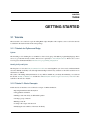
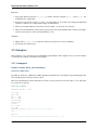
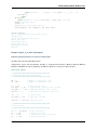
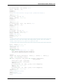
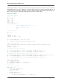
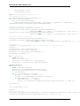
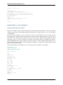
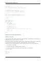
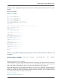
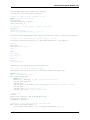
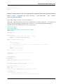
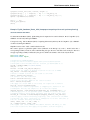
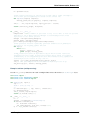
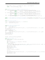
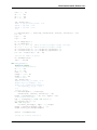
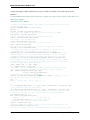
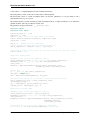
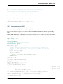
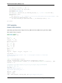
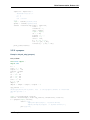
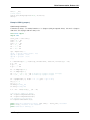
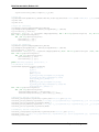
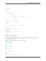
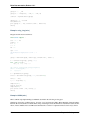
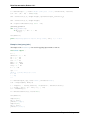
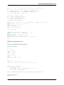
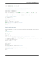
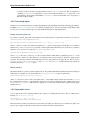
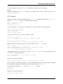
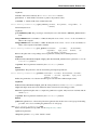
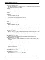
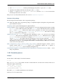
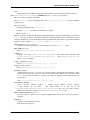
def __call__(self, input):
#the control variables are taken as the last of the buffer
noise_term = input[-1,:]
#update the center frequency by updateing the OU process
self.fc = self.fc-self.fc/tau_i*self.deltaT+noise_term
w0 = 2*pi*self.fc/samplerate
#update the coefficient of the biquadratic filterbank
alpha = sin(w0)*sinh(log(2)/2*self.BW*w0/sin(w0))
self.target.filt_b[:, 0, 0] = sin(w0)/2
self.target.filt_b[:, 1, 0] = 0
self.target.filt_b[:, 2, 0] = -sin(w0)/2
self.target.filt_a[:, 0, 0] = 1+alpha
self.target.filt_a[:, 1, 0] = -2*cos(w0)
self.target.filt_a[:, 2, 0] = 1-alpha
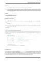
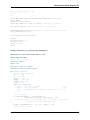
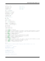
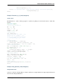
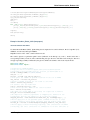
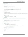
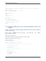
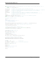
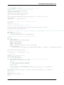
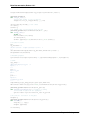
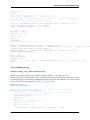
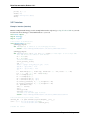
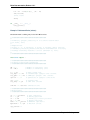
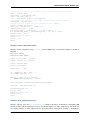
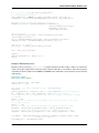
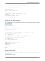
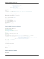
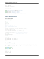
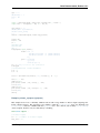
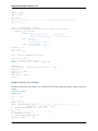
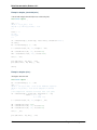
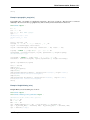
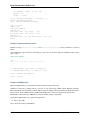
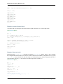
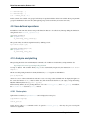
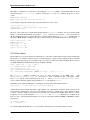
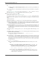
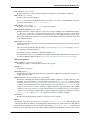
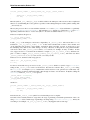
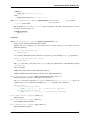
# In the present example the time varying filter is a LinearFilterbank therefore
#we must initialise the filter coefficients; the one used for the first buffer computation
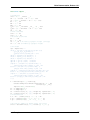
w0 = 2*pi*fc_init/samplerate
BW = 2*arcsinh(1./2/Q)*1.44269
alpha = sin(w0)*sinh(log(2)/2*BW*w0/sin(w0))
filt_b = zeros((nchannels, 3, 1))
filt_a = zeros((nchannels, 3, 1))
filt_b[:, 0, 0] = sin(w0)/2
filt_b[:, 1, 0] = 0
filt_b[:, 2, 0] = -sin(w0)/2
filt_a[:, 0, 0] = 1+alpha
filt_a[:, 1, 0] = -2*cos(w0)
filt_a[:, 2, 0] = 1-alpha
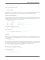
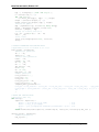
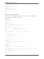
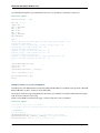
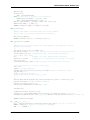
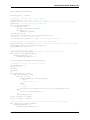
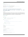
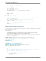
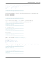
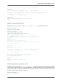
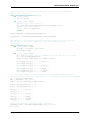
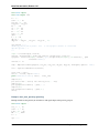
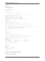
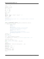
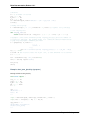
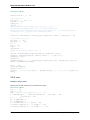
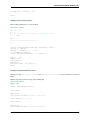
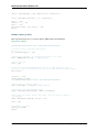
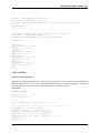
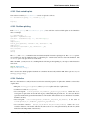
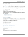
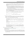
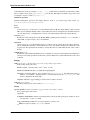
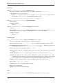
#the filter which will have time varying coefficients
bandpass_filter = LinearFilterbank(sound, filt_b, filt_a)
#the updater
updater = CoeffController(bandpass_filter)
#the controller. Remember it must be the last of the chain
control = ControlFilterbank(bandpass_filter, noise_generator, bandpass_filter,
updater, update_interval)
time_varying_filter_mon = control.process()
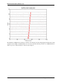
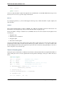
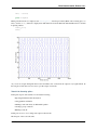
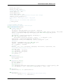
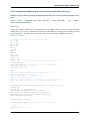
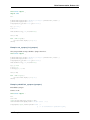
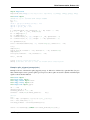
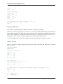
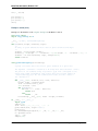
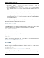
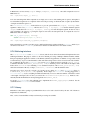
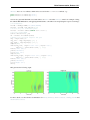
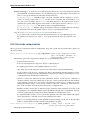
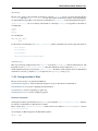
figure(1)
pxx, freqs, bins, im = specgram(squeeze(time_varying_filter_mon),
NFFT=256, Fs=samplerate, noverlap=240)
imshow(flipud(pxx), aspect=’auto’)
show()
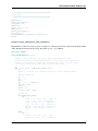
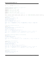
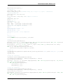
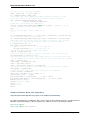
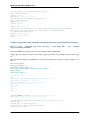
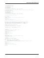
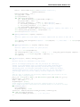
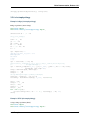
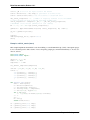
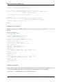
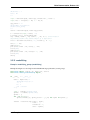
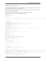
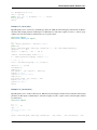
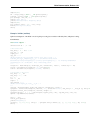
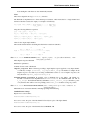
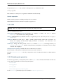
Example: sound_localisation_model (hears)
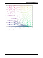
Example demonstrating the use of many features of Brian hears, including HRTFs, restructuring filters and integration
with Brian. Implements a simplified version of the “ideal” sound localisation model from Goodman and Brette (2010).
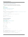
The sound is played at a particular spatial location (indicated on the final plot by a red +). Each location has a
corresponding assembly of neurons, whose summed firing rates give the sizes of the blue circles in the plot. The most
3.2. Examples
109