1
HSC 8 - Mass Balance
January 27, 2015
Research Center, Pori / Antti Remes, Jaana
Tommiska, Pertti Lamberg
14023-ORC-J
1 (29)
51. Mass Balance Module
TOC:
51.1. Where do we need mass balancing?........................................................................... 2
51.2. Mass balancing capabilities in HSC Chemistry® 8 ...................................................... 3
51.3. Overview of the HSC Sim 8 Mass Balancing tool ........................................................ 5
51.4. Step-by-step example: data reconciliation and mass balancing in HSC 8 ................... 6
51.4.1. Drawing the flowsheet .......................................................................................... 6
51.4.2. Importing the experimental data ........................................................................... 6
51.4.3. Reviewing and complementing the data ............................................................... 9
51.4.4. Setting the measurement accuracies ................................................................. 11
51.4.5. Mass balancing .................................................................................................. 13
51.4.6. Reporting and reviewing the results ................................................................... 15
51.4.7. Importing HSC7 Excel files ................................................................................. 16
51.5. Mass balance buttons and dropdowns ...................................................................... 19
51.6. Error check messages ............................................................................................... 22
51.7. Mathematics and algorithms ...................................................................................... 23
51.7.1. Unsized (bulk) mass balance ............................................................................. 23
51.7.2. Sized mass balance (without sized analyses) .................................................... 25
51.7.3. Sized by assay mass balance ............................................................................ 26
51.8. References ................................................................................................................ 29
Copyright © Outotec Oyj 2015
HSC 8 - Mass Balance
January 27, 2015
Research Center, Pori / Antti Remes, Jaana
Tommiska, Pertti Lamberg
51.1.
14023-ORC-J
2 (29)
Where do we need mass balancing?
Mass balancing is a common practice in metallurgy. The mass balance of a circuit is
needed for several reasons:
1.
2.
3.
4.
To estimate the metallurgical performance of the circuit
To locate process bottlenecks and for circuit diagnosis
To create models of the processing stages
To simulate the process.
The following steps are often required to simulate a process:
1.
2.
3.
4.
Collecting experimental data (experimental work, sampling, sample preparation,
assaying)
Mass balancing and data reconciliation of the experimental data
Model building
Simulation.
In HSC Chemistry® 8, you can do all the steps in one program: HSC Sim with the Mass
Balance tool. The work flow in the HSC Sim and Mass Balance tool starts from a flowsheet
drawing, followed by importing experimental data, performing mass balancing, model fitting
& building (model fitting will be available later on) and simulation (Fig. 1).
Fig. 1. From flowsheet with data through mass balancing to modeling and simulation.
Copyright © Outotec Oyj 2015
HSC 8 - Mass Balance
January 27, 2015
Research Center, Pori / Antti Remes, Jaana
Tommiska, Pertti Lamberg
51.2.
14023-ORC-J
3 (29)
Mass balancing capabilities in HSC Chemistry® 8
HSC 8 allows the user to solve the following mass balance problems (Table 1). There are
three different possibilities for the solution:
- Solids
- Assays only
- Solids and water independently
Liquid flow rates and %solids are solved only if Solve solids and water independently is
chosen. If Assays only is chosen, there must be a Total solids measurements for all the
flows to be balanced.
1.
Unsized
Balance Total Solids flow rates. At least one total solids flow rate measurement must
be given
Balance Total Water/liquid flow rate. This is done by first balancing the Total solids
flow rates and after that the Total Water/liquid flow rate independently
Balance %solids
Balance Solids component assays/Mineral assay. At least one solids component
assay or mineral assay must exist
2.
Sized
Balance Total Solids flow rates for bulk and all the size fractions. At least one total
solids flow rate measurement for bulk must be given
Balance size fraction wt-% for size fractions
Balance Total Water/liquid flow rate for bulk. This is done by first balancing the Total
solids flow rates and after that Total Water/liquid flow rate independently
Balance %solids for bulk
Balance Solids component assays/Mineral assay for bulk. If no solids component
assays/mineral assays exist, the solids component assays/mineral assays for bulk
are not balanced
3.
Sized by assay
Balance Total Solids/Slurry flow rates for bulk and all the size fractions. At least one
total solids/slurry flow rate measurement must be given
Balance size fraction wt-% for size fractions
Balance Total Water/liquid flow rate for bulk. This is done by first balancing the Total
solids flow rates and after that Total Water/liquid flow rate independently
Balance %solids for bulk
Balance Solids component assays/Mineral assay for bulk and the size fractions
Copyright © Outotec Oyj 2015
HSC 8 - Mass Balance
January 27, 2015
Research Center, Pori / Antti Remes, Jaana
Tommiska, Pertti Lamberg
14023-ORC-J
4 (29)
Table 1. Mass balance cases that can be solved with HSC Sim.
Measured or
estimated values
Unsized
Sized
Sized by Assays
Components
Total solids flow rates
X
X
X
Water/Liquid flow rates
X
X
X
Solids component Assay/Mineral
Assay bulk
X
X
X
Solid Component Assays/Mineral
assays Size Fractions
X
%Solids
X
X
X
X
Fraction m%
X
X
Total Solids Flow rate size
fractions
X
X
Copyright © Outotec Oyj 2015
HSC 8 - Mass Balance
January 27, 2015
Research Center, Pori / Antti Remes, Jaana
Tommiska, Pertti Lamberg
51.3.
14023-ORC-J
5 (29)
Overview of the HSC Sim 8 Mass Balancing tool
The HSC Mass Balance tool is started from the HSC 8 Main Menu dialog or from HSC Sim
Menu: Tools
Mass Balance. The window layout consists of: Balancing Navigator,
Working Area, Property Panel, and Upper Buttons.
Fig. 2. Main components of the Mass Balance window.
Copyright © Outotec Oyj 2015
HSC 8 - Mass Balance
January 27, 2015
Research Center, Pori / Antti Remes, Jaana
Tommiska, Pertti Lamberg
51.4.
14023-ORC-J
6 (29)
Step-by-step example: data reconciliation and mass balancing in HSC 8
This step-by-step example shows how to do mass balancing for unsized data, consisting of
the solids flow rates and assayed element (Cu, Ni, S) for a rougher-scavenger flotation
bank. The work starts from HSC Sim 8 by drawing the process flowsheet. The Mass
Balance tool is started from the HSC Sim Tools menu. The steps to import the data and to
balance it follow the left side Balancing Navigator panel (Fig. 2) from top to bottom. More
examples are found in Chapter 52.
51.4.1.
Drawing the flowsheet
First the flowsheet is prepared in HSC Sim 8. In this rougher-scavenger flotation example it
looks as shown in Fig. 3.
You can draw all the streams and units. HSC will create the mass balance equations
according to the available data; therefore, there is no need to draw a flowsheet for mass
balancing only or a new flowsheet every time for different kinds of mass balance problems.
When naming the streams, use identical names to those in your analysis lists. Before
proceeding, please check the stream connections and check the flowsheet for possible
errors.
Fig. 3. HSC Sim flowsheet drawing of a flotation process with rougher and scavenger cells.
51.4.2.
Importing the experimental data
When the flowsheet is ready (i.e. all streams are named properly and connections have
been checked), you can import your experimental data. The following subsections will
concentrate on how to import the data for mass balancing and data reconciliation.
1.
Select units
The units are listed based on the flowsheet drawing figure, but they cannot be edited here.
In this view you can:
Select or deselect the units to be included in the balancing calculation.
Set whether the unit will change the particle size distribution of the solids, e.g.
grinding mills. This selection is needed in sized balancing, to indicate that the fraction
balance will not be held over those units.
Copyright © Outotec Oyj 2015
HSC 8 - Mass Balance
January 27, 2015
Research Center, Pori / Antti Remes, Jaana
Tommiska, Pertti Lamberg
14023-ORC-J
7 (29)
Fig. 4. Experimental Data – Units.
2.
Select streams
The streams are listed based on the flowsheet drawing figure, but they cannot be edited
here.
Here you can:
Select and deselect the streams to be included in the balancing calculation.
Change the stream type:
o Unknown
o Solids/Slurry
o Liquid/Water
By default it is unknown, since the data has not yet been imported. When importing the
data, the type is detected by pressing Detect stream types, but it can be changed here.
Fig. 5. Experimental Data – Streams.
3.
Add variables
Next, the measured variables are added / removed from the upper bar buttons. The
variable name and unit on the list can be edited, and the variable can also be unselected
from balancing if desired. The variable types are listed in Table 2.
Copyright © Outotec Oyj 2015
HSC 8 - Mass Balance
January 27, 2015
Research Center, Pori / Antti Remes, Jaana
Tommiska, Pertti Lamberg
14023-ORC-J
8 (29)
Fig. 6. Experimental Data – Variables.
Table 2. Data types of the variables.
Data type
Abbreviation
Examples
Total solids flow rate
SF
Total t/h, g
Solids component flow rate
SC
Iron t/h, plastic t/h, g
Solids component assay
A
Cu%, P2O5%
Mineral assay
M
Ccp%, Py%, Qtz%
Size Fraction wt %
SA
0-20um %, 20-45um %
Solids percentage
SP
35%
Not included
NA
Column with comments,
extra data (temperature),
etc.
4.
Add size fractions
By default, one size fraction exists: ‘Bulk’, which cannot be removed. More size fractions
can be added to /removed from the list by clicking the buttons on the upper bar. Fraction
names can be given.
Fig. 7. Experimental Data – Size Fractions.
Copyright © Outotec Oyj 2015
HSC 8 - Mass Balance
January 27, 2015
Research Center, Pori / Antti Remes, Jaana
Tommiska, Pertti Lamberg
5.
14023-ORC-J
9 (29)
Add dataset(s)
By default, one dataset exists, which can be renamed here. In addition, more datasets can
be added and selected one at a time to carry out data reconciliation.
Fig. 8. Experimental Data – Datasets.
6.
Import measurement data
In this view, a stream variable template is automatically generated and displayed. The data
can be entered by:
a)
b)
c)
Typing manually in the table
Copying an empty data template
organizing the data e.g. in Excel
select ‘Paste
Experimental Data’. This will automatically place the data in the correct rows and
columns based on the clipboard table content. Note: if the data is horizontal (stream
names in rows) there must exist a column labelled Fraction that contains fraction
names. If the data is vertical (stream names in columns) there must exist a row
labelled Fraction containing the fraction names.
Importing the old HSC7 Analyses.xls mass balance file
Each dataset is presented in a separate table tab.
Fig. 9. Experimental Data – Measurement Data.
51.4.3.
Reviewing and complementing the data
In this part, the idea is to inspect the data and get an understanding of what values will be
available after balancing. Also, the data status before balancing is reviewed here and can
be changed. Thus changes are reflected in the status after balancing.
Copyright © Outotec Oyj 2015
HSC 8 - Mass Balance
January 27, 2015
Research Center, Pori / Antti Remes, Jaana
Tommiska, Pertti Lamberg
14023-ORC-J
10 (29)
The status indications are:
Stream:
• Missing: no data
• Complete: all variables have data
• Partial: some variables have data
Variable:
• Missing: no data
• Measured: data existing
• Guesstimated: data are a user-given guesstimation; high uncertainty is set
automatically for this The guesstimation is given in the property User value
• Fixed: the user sets including the value that you do not wish to change during
the balancing. However, the fixed value may change during balancing because
the fixing is done by setting the uncertainty to small. The fixed value is given in
the property User value
• By Equation: stream total solids can be set to be a multiple of another stream
• Excluded: data will not be included in the calculation
After Balancing:
• Balanced: solved using data reconciliation
• Calculated: calculated based on unit material balance
• Non Available: data are also missing after balancing
The status indications can be changed by clicking the data table cell (dropdown menu) or
from the property panel on the right.
The balance equations for the units can be reviewed by clicking the upper bar button
shown.
Fig. 10. Opening and reviewing the balance equations.
Copyright © Outotec Oyj 2015
HSC 8 - Mass Balance
January 27, 2015
Research Center, Pori / Antti Remes, Jaana
Tommiska, Pertti Lamberg
1.
14023-ORC-J
11 (29)
View by streams
The data are presented in a pivot table where the stream is the major column. The data
status is shown in pie charts.
Fig. 11. Data Status – Stream View
2.
View by variables
The data is presented in a pivot table where the variable is the major column. The data
status is shown in pie charts.
Fig. 12. Data Status – Stream View.
51.4.4.
Setting the measurement accuracies
Each assay and piece of raw data is subject to errors. Mass balancing and data
reconciliation is meant for adjusting unreliable values, whereas reliable values should be
adjusted only a little, if at all. Therefore, the user has to give a value of how reliable each
item of raw data is. This is done by defining the error model to give a standard deviation
value for the measurement data.
In the HSC Sim 8 Mass Balance tool, the standard deviation can be given using userfriendly pre-settings for the error models.
Copyright © Outotec Oyj 2015
HSC 8 - Mass Balance
January 27, 2015
Research Center, Pori / Antti Remes, Jaana
Tommiska, Pertti Lamberg
14023-ORC-J
12 (29)
To define the standard deviations you need to select:
Table 3. Descriptions of error model functions.
Error Model
Parameters
Example
Fixed
Fixed standard deviation as a plain number or fixed
relative standard deviation as a negative number or in
parentheses
0.1
X.x = X%+0.x
The integer is the relative standard deviation; the
decimal is the detection limit
10.1
X%+0.1
Given parameter is the relative standard deviation; 0.1
is the detection limit
6
10%+X
Parameter is the detection limit; relative standard
deviation is fixed at 10%
0.05
a;b;c = MIN(a%+b;c)
a is the relative standard deviation, b is the detection
limit, and c is the maximum standard deviation
10;0.01;0.5
a;b;c=MAX(a%+b;c)
a is the relative standard deviation, b is the detection
limit, and c is the minimum standard deviation
10;0.02;0.2
a;b;c=%;MIN;MAX
a is the relative standard deviation, MIN is the
minimum standard deviation, and MAX is the
maximum standard deviation
10;
Manual
Standard deviation is given in the data individually for
each stream
1.
-5, (5)
Standard deviations by streams
The data are presented in a pivot table where the stream is the major column. Standard
deviation settings of all variables for that stream can be easily set at once.
Fig. 13. Standard Deviations – SD – Stream View.
2.
Standard deviations by variables
The data are presented in a pivot table where the variable is the major column. Standard
deviation settings of all streams for that variable can be easily set at once.
Copyright © Outotec Oyj 2015
HSC 8 - Mass Balance
January 27, 2015
Research Center, Pori / Antti Remes, Jaana
Tommiska, Pertti Lamberg
14023-ORC-J
13 (29)
Fig. 14. Standard Deviations – SD – Variable View.
51.4.5.
Mass balancing
In the mass balancing upper bar, the following can be selected:
Sum = 100: if the mineral component sum is required to be 100%.
Method: LS, NNLS, CLS
Data to Balance: Assays only, Solids and assays, Solids and water
PSD Balance: Unsized, Sized, Sized by Assay
Calculate: runs the data reconciliation
The balancing results can be viewed graphically with, see Fig. 15:
Balance Convergence
Parity Chart
To solve a mass balance problem, the following mathematical methods are available in the
Balance/Report Options on the right-hand side:
Least Squares Solution (LS)
Non-negative Least Squares Solution (NNLS)
Constrained Least Squares Solution (CLS)
Copyright © Outotec Oyj 2015
HSC 8 - Mass Balance
January 27, 2015
Research Center, Pori / Antti Remes, Jaana
Tommiska, Pertti Lamberg
14023-ORC-J
14 (29)
Fig. 15. Balancing – Calculate.
Mass balance problems are solved in two stages: firstly, the total mass flow rates are
solved and then the assays are reconciled. In solving the assays, the least squares solution
finds the best solution by minimizing the weighted sum of squares, i.e.
k
n
j 1
i 1
WSSQ
aij
bij
sij
2
2
(1)
where j refers to the stream, k is the number of streams, i refers to the components
(analyses), n is the number of components, a is the measured value, b is the balanced
value, and s is the standard deviation.
In non-negative least squares, all ‘a’s are subject to being non-negative.
In constrained least squares, all ‘a’s are subject to being between the min. and max.
By clicking dataset you can see the solution parameters Balance tolerance, Max iter and
Estimate of null SD in the properties window. Balance tolerance is the condition that defines
when the iterations stop and Max iter is the maximum number of iterations. If you don’t get
reasonable balance you can try to change Estimate of null SD greater.
Copyright © Outotec Oyj 2015
HSC 8 - Mass Balance
January 27, 2015
Research Center, Pori / Antti Remes, Jaana
Tommiska, Pertti Lamberg
51.4.6.
14023-ORC-J
Reporting and reviewing the results
Fig. 16. Stream Summary
Fig. 17. Reporting – Results: Goodness.
Copyright © Outotec Oyj 2015
15 (29)
HSC 8 - Mass Balance
January 27, 2015
Research Center, Pori / Antti Remes, Jaana
Tommiska, Pertti Lamberg
14023-ORC-J
16 (29)
Fig. 18. Reporting – Unit Balance.
51.4.7.
Importing HSC7 Excel files
The Excel files to be imported may contain a sheet with flowsheet information (Fig. 19). If
this sheet is named Flowsheet, the program automatically detects the sheet where the
flowsheet information is located. If the name is something else or there is no sheet
containing flowsheet information, the name must be specified (Fig. 23, Select Flowsheet)
Fig. 19. An Excel sheet containing flowsheet data.
The measurement data is read from a different sheet of the same Excel file. The first
column must be named Streams (Cell A1), the second Source (Cell A2), and the third
Destination (cell A3) if the data are horizontal (Fig. 21). If the data are vertical, the first row
must be named Streams (A1), the second row must be named Source (A2), and the third
Destination (A3) (Fig. 20). Imported vertical data can only be unsized or sized (without
analyses).
Copyright © Outotec Oyj 2015
HSC 8 - Mass Balance
January 27, 2015
Research Center, Pori / Antti Remes, Jaana
Tommiska, Pertti Lamberg
14023-ORC-J
17 (29)
Fig. 20. Vertical sized data (without analyses).
Fig. 21. Horizontal unsized data.
The program automatically detects a sheet named Streams as the sheet where the
measurement data can be found. If the name of the sheet containing the measurement data
is not Streams, the user should tell the program where the measurement data can be found
(Fig. 23, Analyses)
The following screenshots show how an HSC7 file is imported. Importing an HSC7 file is
started by clicking Tools-Mass Balancing and then clicking the Import HSC7 Data button
(Fig. 22). After that a dialog will open (Fig. 23).
Copyright © Outotec Oyj 2015
HSC 8 - Mass Balance
January 27, 2015
Research Center, Pori / Antti Remes, Jaana
Tommiska, Pertti Lamberg
14023-ORC-J
Fig. 22. Import HSC7 Data.
Fig. 23. Import HSC7 Data Dialog.
Copyright © Outotec Oyj 2015
18 (29)
HSC 8 - Mass Balance
January 27, 2015
Research Center, Pori / Antti Remes, Jaana
Tommiska, Pertti Lamberg
51.5.
14023-ORC-J
19 (29)
Mass balance buttons and dropdowns
Update and save changes to HSC Sim flowsheet and close
Discard changes and close HSC mass balance
Open/Save backup (HSCMas file) of the mass balance
Import existing HSC7 mass balance data (analyses.xls)
Error check
Help and examples
Detects stream types automatically for Solid/slurry and Liquid based
on the data. If there are streams with no data the stream type is set as
Unknown. The user should either uncheck these Unknown streams or
set the types manually
Select elements from periodic table
Select minerals from HSC database
Add new variable
Copyright © Outotec Oyj 2015
HSC 8 - Mass Balance
January 27, 2015
Research Center, Pori / Antti Remes, Jaana
Tommiska, Pertti Lamberg
14023-ORC-J
20 (29)
Remove the selected variable
Add a new sieve size
Add a new data set
Remove the selected data set
Transpose streams and variables
Copy the whole table
Paste data to correct places based on the stream and variable names
Element to mineral conversion using HSC Geo
View minerals and their compositions
Converts solids percentage measurements to water flow rates
Back calculate missing data if possible
Clear back calculated missing data
Copyright © Outotec Oyj 2015
HSC 8 - Mass Balance
January 27, 2015
Research Center, Pori / Antti Remes, Jaana
Tommiska, Pertti Lamberg
14023-ORC-J
21 (29)
View the mass balance equations
Unselect the streams without data
Exclude all elements (A) and do balancing with minerals (M)
Set component sum=100 when balancing minerals
Select calculation method. The available methods are LS, NNLS, and
CLS
PSD balance: Possible selections are Unsized, Sized and Sized by
Assays
Select the data to be balanced
Calculates mass balance
Clears the mass balancing results
Create or update HSC Sim stream tables
Copyright © Outotec Oyj 2015
HSC 8 - Mass Balance
January 27, 2015
Research Center, Pori / Antti Remes, Jaana
Tommiska, Pertti Lamberg
51.6.
14023-ORC-J
22 (29)
Error check messages
1.
Dataset: No Active dataset found
Please contact the developers
2.
Units: No selected units found
At least one unit should be selected
3.
Streams: No selected streams found
Some of the streams should be selected
4.
Units: No input stream
Found a unit with no input streams
5.
Units: No output stream
Found a unit with no output streams
6.
Streams: Source and destination missing
Found a stream with no source and destination
7.
Fractions: Bulk not found
Please contact the developers
8.
Data: No data found
Add data in the measurement data view
9.
Variables: Total solids measurement missing
There should be exactly one selected variable of the Total Solids type
10.
Variables: Too many variables of the type total solids
There should be exactly one selected variable of the Total Solids type
11.
Variables: No selected assays found
There should be at least one selected variable of the Mineral Assay or Solids
Component Assay type
12.
Streams: All stream types unknown
Go to Streams and press Detect Stream Types button or set the stream types
manually
13.
User Values: UserValues missing
ValueStatus of some data is set to Fixed or Questimated but the UserValue is
not given
14.
Stream Types: Unknown found
Go to Streams and press Detect Stream Types button or set the stream types
manually
15.
Variables: Size Fraction wt % variable missing
There should be exactly one variable of the type Size Fraction wt %
16.
Variables: Too many variables of the type Size Fraction wt-%
There should be exactly one variable of the type Size Fraction wt %
17.
Units: No combined units found
There can be several reasons why combined units cannot be formed. There may
be too many missing measurements or there may be errors in the flowsheet.
18.
Notification: Min or Max values detected: It is recommended to use the CLS method
Copyright © Outotec Oyj 2015
HSC 8 - Mass Balance
January 27, 2015
Research Center, Pori / Antti Remes, Jaana
Tommiska, Pertti Lamberg
51.7.
14023-ORC-J
23 (29)
Mathematics and algorithms
In this section, the main algorithms and methods for data reconciliation in HSC Chemistry®
8 are briefly summarized.
Definitions
NF1
NF2
NU
NSRU
NSF
NE
G
GM
F
FM
W
WM
Pc
PcM
M
MM
=
=
=
=
=
=
=
=
=
=
=
=
=
=
=
=
number of flows, unsized
number of flows, sized, sized by assay
number of units
number of size-reducing units (PSD changing unit)
number of sub-flows
number of chemical elements
grade of chemical element
measured grade of chemical element
solids flow rate
measured solids flow rate
water flow rate
measured water flow rate
%solids = F*100/(F + W)
measured %solids
fraction m% = Fflow,subflow*100/Fflow
fraction m% measurements
1, the flow enters the unit
e unit
flow
1, the flow exits
the unit
0, otherwise
51.7.1.
Unsized (bulk) mass balance
In the unsized (bulk) mass balance solution, solids and water flow rates are solved first.
After that the bulk analyses are solved. During the calculation: 1) the solids flow rates are
solved first and after that 2) the water flow rates are solved.
1.
Bulk flow rates
The equations for solving the bulk solids flow rate are:
mass balance Equations (2)
NF 1
unit
eflow
* Fflow ,tot
0
unit
1,.., NU
flow 1
analyses Equation (3)
Copyright © Outotec Oyj 2015
(2)
HSC 8 - Mass Balance
January 27, 2015
Research Center, Pori / Antti Remes, Jaana
Tommiska, Pertti Lamberg
NF 1
14023-ORC-J
M
unit
eflow
* Gflow
,tot ,chemical _ element * Fflow ,tot
0 unit
24 (29)
1,..., NU
(3)
flow 1
chemical _ element
1,..., N E
solids flow rate measurements (4)
Fflow ,tot
M
Fflow
,tot
flow
(4)
1,..., NF 1
The equations for solving the bulk water flow rate are:
mass balance Equations (5)
NF 1
unit
eflow
* Wflow ,tot
0
unit
1,.., NU
(5)
flow 1
water flow rate measurements Equation (6)
Wflow ,tot
M
Wflow
,tot
flow
(6)
1,.., NF 1
% solids measurements (7)
(Pc M / 100 ) * W flow ,tot
Fflow ,tot
(Pc M / 100 ) * Fflow ,tot
flow
1,.., N F 1
(7)
Mass balance Equations (2) and (5) are the equality constraints for the solutions. The
solution method used is element-wise weighted total least squares2. The weights are
standard deviations of the solids flow rate measurements FM, the analyses GM, the water
flow rate measurements WM, and the %solids measurements PcM. The flow rates can be
solved without any constraints (LS), subject to non-negativity constraints (NNLS)3 ,and
subject to simple bounds
lb1 F ub1
lb2 W ub2
(CLS)4.
2.
Bulk analyses
Let G and GM be NF1 x NE matrices. The operator vec stacks the matrix columns into a
vector.
The equations for the analyses solution are:
measurements (8)
vec(G) vec(GM )
(8)
mass balance Equations (9) for the analyses:
vec (B * G )
0
(9)
where the NU x NF1 matrix B is defined:
Copyright © Outotec Oyj 2015
HSC 8 - Mass Balance
January 27, 2015
Research Center, Pori / Antti Remes, Jaana
Tommiska, Pertti Lamberg
Bunit ,flow
14023-ORC-J
25 (29)
flow
eunit
* Fflow ,tot
(10)
If the option minerals sum=100 is selected, the following Equations (11) are included:
NE
Gflow ,tot ,chemical _ element
chemicalelement 1
100
flow
1,..., NF 1
(11)
Equations (9) and (11) are the equality constraints for the solution. The solution method
used is weighted least squares 1). If Equations (11) are included in Equations (9), the
matrix B is (NU – 1) x NF1 to avoid linear dependency of equality constraints.
As before, the analyses can be solved without any constraints (LS), subject to nonnegativity constraints (NNLS), and subject to simple bounds (CLS). If there are no
constraints, the minimal maximum norm solution can be calculated (LS, MinMax)5.
51.7.2.
Sized mass balance (without sized analyses)
Sized mass balance differs from unsized (bulk) solution in that the fraction m% is solved
and the fraction m% measurement is used in the solution of total flows. Sized differs from
Size by Assay in that the analyses are not given and the number of flows is the same as in
the unsized case.
1.
Total flow mass balances of the streams
Firstly, the total flows are solved. The Equations are:
mass balance Equations (12)
NF 1
unit
eflow
* Fflow ,tot
0
unit
1,.., NU
(12)
flow 1
fraction m% measurements (13)
NF 1
M
unit
eflow
* Mflow
,subflow * Fflow ,tot
0
unit
1,..., NU
NSRU
1
(13)
flow 1
subflow
1,.., NSF
Units are indexed up to NU - NSRU - 1 to avoid linear dependency of equality constraints.
Flow measurements (14)
Fflow ,tot
M
Fflow
,tot
flow
(14)
1,..., NF 1
If 1D analyses are given, the following Equations are included:
analyses (15)
NF 1
M
unit
eflow
* Gflow
,tot ,chemical _ element * Fflow ,tot
0 unit
1,..., NU
(15)
flow 1
chemical _ element
Copyright © Outotec Oyj 2015
1,..., N E
HSC 8 - Mass Balance
January 27, 2015
Research Center, Pori / Antti Remes, Jaana
Tommiska, Pertti Lamberg
14023-ORC-J
26 (29)
Equations (12) are equality constraints for the solution. The solution method used is
element-wise weighted total least squares. The weights are standard deviations of the
solids flow rate measurements FM, the analyses GM and fraction m% MM.
As before, the flow rates can be solved without any constraints (LS), subject to nonnegativity constraints (NNLS), and subject to simple bounds (CLS). If there are no
constraints, the minimal maximum norm solution can be calculated (LS, MinMax)5.
2.
Size fraction flow mass balance
Then the %m values of the sub-flows are solved. The equations are:
fraction m% measurements (16)
M flow ,subflow
M
Mflow
,subflow
(16)
mass balance equations (17)
NF 1
unit
eflow
* M flow ,subflow * Fflow,tot
unit
0
1,..., NU unit not size reducing
flow 1
subflow
(17)
1,.., N SF
sum fraction m% is a hundred (18)
NSF
Mflow ,subflow
100
(18)
i 1
Equations (17) and (18) are equality constraints. The solution method used is element-wise
total least squares and %m values can be solved without any constraints (LS), subject to
non-negativity constraints (NNLS), and subject to simple bounds (CLS).
3.
Bulk analyses
If the unsized bulk analyses are given, the balanced analyses are calculated as described
above (see: unsized mass balance).
51.7.3.
Sized by assay mass balance
Before a sized by assay mass balance solution, the unsized or sized mass balance must be
solved first. The results Fflow,tot of the unsized or sized solution are used in the sized by
assay solution. In a sized by assay solution, the size fraction sub-flows are calculated first
and after that the analyses are solved.
1.
Sized by assay fraction sub-flows
The equations for size by assay sub-flow solutions are:
mass balance Equations (19) for each unit that is not size reducing
NF 2
unit
eflow
* Fflow ,subflow
0
unit
n1,..., nNU
1
unit not size reducing
(19)
flow 1
subflow
1,.., NS
Copyright © Outotec Oyj 2015
HSC 8 - Mass Balance
January 27, 2015
Research Center, Pori / Antti Remes, Jaana
Tommiska, Pertti Lamberg
14023-ORC-J
27 (29)
Above ni is the index of the ith unit that is not size reducing. Units are indexed up to NU - 1
to avoid linear dependency of equality constraints.
Sum of sub-flows is the total flow (20)
NS
Fflow ,subflow
subflow 1
Fflow ,tot
flow
1,..., NF 2
(20)
Analyses for each unit that are not size reducing (21)
NF 2
unit
eflow
* Gflow ,chemical _ element ,sublow * Fflow ,subflow
0
flow 1
unit
n1,..., nNU
unit not size reducing
chemical _ element
subflow
(21)
1,..., NE
1,.., NS
Fraction %m measurements (22)
Fflow ,subflow
flow
M
Mflow
,subflow * Fflow ,tot / 100
(22)
1,..., NF 2
subflow
1,.., NS
or alternatively
flow measurements (23)
Fflow ,subflow
flow
M
Fflow
,subflow
(23)
1,..., NF 2
subflow
1,..., NS
The solution method used is element-wise weighted least squares. The equations can be
solved without any constraints (LS), subject to non-negativity constraints (NNLS), and
subject to simple bounds (CLS).
2.
Sized by assay fraction analyses
Let G and GM be NF2*NS x NE matrices. The operator vec stacks the matrix columns into a
vector.
The equations for the analyses solution are:
vec(G) vec(GM )
(24)
mass balance equations (25) for the analyses
vec (B * G )
0
(25)
where the (NS - 1)*(NU - NSRU)x(NF2*(NS - 1)) matrix B is defined
B
diag (B subflow )
sublow
1,.., NS 1
Copyright © Outotec Oyj 2015
(26)
HSC 8 - Mass Balance
January 27, 2015
Research Center, Pori / Antti Remes, Jaana
Tommiska, Pertti Lamberg
14023-ORC-J
28 (29)
Sub-flows are indexed up to NS - 1 to avoid linear dependency of equality constraints.
Where the operator diag adds matrices Bsubflow at the diagonal of the matrix B and
sublow
Bunit
,flow
unit
eflow
* Fflow ,subflow
(27)
the sum of sub-flows is the total flow (28)
NS
Fflow ,subflow
subflow 1
* Gflow ,chemical _ element,subflow
Fflow ,tot * Gflow ,tot,chemical _ element
flow
(28)
1,..., N F 2
chemical _ element
1,..., NE
If the option minerals sum=100 is selected, the following Equations (29) are included:
NE
Gflow ,chemical _ element ,subflow
chemicalelement 1
100
flow
1,..., NF 1
(29)
subflow
1,...,NS
If Equations (29) are included, B is (NS - 1)*(NU - NSRU - 1)x(NF2*(NS - 1))
to avoid linear dependencies.
The solution method used is weighted least squares. The equations can be solved without
any constraints (LS), subject to non-negativity constraints (NNLS), and subject to simple
bounds (CLS).
Copyright © Outotec Oyj 2015
HSC 8 - Mass Balance
January 27, 2015
Research Center, Pori / Antti Remes, Jaana
Tommiska, Pertti Lamberg
51.8.
14023-ORC-J
29 (29)
References
1.
2.
3.
4.
5.
Golub, van Loan: Matrix Computations, Third edition 1996
Markovsky, Rastello, Premoli, Kuhush, van Huffel: The element-wise weighted total
least squares problem, Computational Statistic & Data Analysis 50 (2006) pp.181-209
Lawson, Hanson: Solving Least Squares Problems, 1974
Haskell, Hanson: An Algorithm for Linear Least Squares Problems with Equality
and Nonnegativity Constraints, Mathematical Programming 21 (1981), pp.98-118
Barrodale, Phillips: Algorithm 495, Solution of an Overdetermined System of Linear
Equations in the Chebyshev Norm, ACM Transactions on Mathematical Software, Vol
1, No 3, September 1975, pp. 264-270.
Copyright © Outotec Oyj 2015