Download Introduction To Embedded Systems Development

Introduction To Embedded Systems Development
Rohit Ramesh
Contents
1 Introduction
1.1
3
Resources . . . . . . . . . . . . . . . . . . . . . . . . . . . . . . . . . . . . . . . . . . . . . . .
2 GPIO
3
4
2.1
Prequisites
. . . . . . . . . . . . . . . . . . . . . . . . . . . . . . . . . . . . . . . . . . . . . .
4
2.2
What is GPIO? . . . . . . . . . . . . . . . . . . . . . . . . . . . . . . . . . . . . . . . . . . . .
4
2.3
GPIO Output . . . . . . . . . . . . . . . . . . . . . . . . . . . . . . . . . . . . . . . . . . . . .
4
2.4
GPIO Input . . . . . . . . . . . . . . . . . . . . . . . . . . . . . . . . . . . . . . . . . . . . . .
7
2.5
Project : Bit Banging . . . . . . . . . . . . . . . . . . . . . . . . . . . . . . . . . . . . . . . .
11
3 Clocking
13
3.1
Clock Dividers . . . . . . . . . . . . . . . . . . . . . . . . . . . . . . . . . . . . . . . . . . . .
13
3.2
Phase Locked Loops . . . . . . . . . . . . . . . . . . . . . . . . . . . . . . . . . . . . . . . . .
14
3.3
Calculating Clock Speed . . . . . . . . . . . . . . . . . . . . . . . . . . . . . . . . . . . . . . .
15
3.4
Working Backwards . . . . . . . . . . . . . . . . . . . . . . . . . . . . . . . . . . . . . . . . .
16
3.5
Making The Changes . . . . . . . . . . . . . . . . . . . . . . . . . . . . . . . . . . . . . . . . .
17
3.6
Peripheral Clocks . . . . . . . . . . . . . . . . . . . . . . . . . . . . . . . . . . . . . . . . . . .
20
3.7
Project : Precision Timing . . . . . . . . . . . . . . . . . . . . . . . . . . . . . . . . . . . . . .
20
4 Timers
22
4.1
Basic Description . . . . . . . . . . . . . . . . . . . . . . . . . . . . . . . . . . . . . . . . . . .
22
4.2
Speed Settings . . . . . . . . . . . . . . . . . . . . . . . . . . . . . . . . . . . . . . . . . . . .
22
4.3
Match Registers . . . . . . . . . . . . . . . . . . . . . . . . . . . . . . . . . . . . . . . . . . . .
24
4.4
Capture Registers . . . . . . . . . . . . . . . . . . . . . . . . . . . . . . . . . . . . . . . . . . .
25
4.5
Project : Serial Light Communications . . . . . . . . . . . . . . . . . . . . . . . . . . . . . . .
26
1
5 ADC
28
5.1
Theory of Operation . . . . . . . . . . . . . . . . . . . . . . . . . . . . . . . . . . . . . . . . .
28
5.2
Basic Usage . . . . . . . . . . . . . . . . . . . . . . . . . . . . . . . . . . . . . . . . . . . . . .
28
5.3
Interrupts . . . . . . . . . . . . . . . . . . . . . . . . . . . . . . . . . . . . . . . . . . . . . . .
30
5.4
Connecting to Timers . . . . . . . . . . . . . . . . . . . . . . . . . . . . . . . . . . . . . . . .
31
5.5
Burst Mode . . . . . . . . . . . . . . . . . . . . . . . . . . . . . . . . . . . . . . . . . . . . . .
31
5.6
DMA
. . . . . . . . . . . . . . . . . . . . . . . . . . . . . . . . . . . . . . . . . . . . . . . . .
31
5.7
Project : Optical Theramin . . . . . . . . . . . . . . . . . . . . . . . . . . . . . . . . . . . . .
31
6 DAC
41
6.1
Working Theory . . . . . . . . . . . . . . . . . . . . . . . . . . . . . . . . . . . . . . . . . . .
41
6.2
Usage . . . . . . . . . . . . . . . . . . . . . . . . . . . . . . . . . . . . . . . . . . . . . . . . .
41
7 DMA
42
7.1
GPDMA in the LPC . . . . . . . . . . . . . . . . . . . . . . . . . . . . . . . . . . . . . . . . .
43
7.2
DMA with the ADC . . . . . . . . . . . . . . . . . . . . . . . . . . . . . . . . . . . . . . . . .
43
7.3
DMA with the DAC . . . . . . . . . . . . . . . . . . . . . . . . . . . . . . . . . . . . . . . . .
43
7.4
DMA and Power Control
. . . . . . . . . . . . . . . . . . . . . . . . . . . . . . . . . . . . . .
44
7.5
Project : Sound Recorder . . . . . . . . . . . . . . . . . . . . . . . . . . . . . . . . . . . . . .
44
7.6
Suggested Steps . . . . . . . . . . . . . . . . . . . . . . . . . . . . . . . . . . . . . . . . . . . .
44
7.7
Microphone Circuit . . . . . . . . . . . . . . . . . . . . . . . . . . . . . . . . . . . . . . . . . .
44
8 Appendix
48
8.1
Development Environment Setup . . . . . . . . . . . . . . . . . . . . . . . . . . . . . . . . . .
48
8.2
Standard Macros . . . . . . . . . . . . . . . . . . . . . . . . . . . . . . . . . . . . . . . . . . .
54
2
1
Introduction
This book will teach you embedded system design and development, using the LPC1769, an ARM Cortex
microcontroller. When compared to normal CPU the LPC is a simple device, with only one processor core
and a miniscule amount of memory, yet it still manages to be useful. In fact this simplicity makes it a
wonderful learning tool, allowing us to forgo kernel and driver interfaces and work at the lowest level possible,
without becoming too complicated to dive headfirst into. We’ll exploit the simplicity to teach you about
how processors are structured, how to deal with many common protocols and tools, and even how some
fundamental parts of an operating system work.
The LPC itself has a number of modules, which encapsulate various features of the processor. We’ll be
working our way through those modules, explaining why you would use them, how they work, and how to use
them. With each module we learn about, we’ll present exercises and projects that will help you cement that
knowledge, and give you a practical examples of how these devices can be used.
While we’ll often be working with electronics, no initial knowledge is required, and we’ll give you the resources
to learn what you need to know as you go along.
1.1
Resources
This textbook will mainly work to help you build a conceptual framework around these topics, there are
other resources that will give you the fine detail.
1.1.1
The LPC 17XX User Manual
The User Manual (available here1 ) will be the main document this textbook builds on. It contains detailed
information on all of the available features of the LPC, and how you can use them.
Though this textbook is meant to give you all of the background that the manual lacks, it is in no way a
substitute. There will be a lot we cannot actually go over and to get the most out of this course, after every
chapter you read in this textbook, you should read the corresponding chapters in the manual.
A quick warning, this manual is very large, and you should not print it unless it’s absolutely necessary.
1.1.2
The LPC1769 Schematic
The schematic (available here 2 ) describes how the pins on the development boards correspond to the pins
mentioned in the manual. You’ll need to cross reference this schematic with Chapter 8 of the manual every
time you need to figure out the physical location of any one particular pin.
1.1.3
The LPC176X Data Sheet
The data sheet (available here3 ) is the last reference document you should keep handy. It contains a lot of
information about the limitations of the LPC, the tolerances of various features, and the full set of features
the LPC has.
1 http://www.nxp.com/documents/user_manual/UM10360.pdf
2 http://www.cs.umd.edu/class/fall2012/cmsc498a/manuals/lpcxpresso_lpc1769_schematic.pdf
3 http://www.nxp.com/documents/data_sheet/LPC1769_68_67_66_65_64_63.pdf
3
2
GPIO
2.1
Prequisites
Read the following tutorials to get you up to speed with the electronics:
•
•
•
•
How to read a schematic
How to use a breadboard
Understanding LEDs
Using Pull Up Resistors
All these tutorials are Arduino centric, but you can extrapolate to what you need to do for your LPC.
2.2
What is GPIO?
We’ll start with the most basic peripheral on the LPC, General Purpose Input Output. GPIO is what lets
your microcontroller be something more than a weak auxiliary processor. With it you can interact with the
environment, connecting up other devices and turning your microcontroller into something useful.
GPIO has two fundamental operating modes, input and output. Input lets you read the voltage on a pin, to
see whether it’s held low (0v) or high (3v) and deal with that information programmatically. Output lets you
set the voltage on a pin, again either high or low. Every pin on the LPC can be used as a GPIO pin, and can
be independently set to act as an input or output.
In this chapter we will show how to complete 2 tasks, reading the state of a button, and making an LED
blink. Using what you learn from that, you’ll be able to start building more complex devices, and even
implementing simple communications protocols.
2.3
GPIO Output
GPIO output is a versatile and powerful tool, especially given that it takes little effort to use and control it.
Once you’ve chosen a pin, the process to use it is straightforward:
• tell the LPC that the pin should be used as an output
• tell the LPC whether the pin should be held low or high.
The interesting part is how exactly you can give the LPC instructions, and what it does in order to carry
them out.
2.3.1
Memory Mapped Registers
In order to talk to the GPIO controller, or any other peripheral, we have we have to use memory mapped
registers. In most computers these low level interfaces are hidden by the kernel, and often only higher
level interfaces are available to developers. The LPC however doesn’t have a kernel or drivers hiding these
interfaces from you. This gives you the ability to work with them directly, without having to deal with the
virtual device abstraction a modern OS would impose.
When we try to read or write to a normal chunk of memory, the address and instruction are sent to the
memory controller. The memory controller then either retrieves data from memory and places it into a
4
register, or takes data from a register and writes it to somewhere in the memory. However, there are a number
of privileged address, and when you try to read from or write to these a different pathway is taken. Here
when the memory controller gets the instruction it notices the address is special, and instead of going to the
memory module, it’ll forward the request to a register that’s located in the relevant peripheral.
These registers all have different functions, each of which is detailed in the manual along with the register’s
memory address. The really important thing to notice is that you’re not dealing with a normal piece of
memory, and these memory mapped registers can act very differently.
Unlike static memory where you can read or write pretty much anywhere, there are a number of these memory
mapped registers which you can only read from. Trying to write to any of these will trap your system in a
hard fault. Neither can you rely on the assumption that reads are nondestructive. There are some registers
which are connected to FIFOs and other structures, and reading from them is the same as popping from
that queue, and the next time you read from the same address, you’ll get a different value. Even the usual
guarantee that a write operation is idempotent is lost. There are registers where a write operation will trigger
some change in the peripheral, making the LPC turn an LED on, or send out a signal.
2.3.2
Blinking Lights
So let’s start with something simple: Blinking Lights. Connect up an LED to pin P0[9] and ground, making
sure to place the proper current limiting resistor in series with it. To actually turn on the LED you have to
first tell the LPC that the pin is to be used for output, and then set the state to be on. If you look in the
manual you’ll see that P0[9]’s direction is controlled by the 9th bit in a register located at 0x2009C000, and
that setting it to 1 makes it an output pin. 4
((uint32_t *) 0x2009C000) |= (1 << 9); // Set P0[9] to output
Then there’s another register at 0x2009C014 which controls the state of the pin, so we can turn turn the
light on and off by manipulating its 9th bit.
((uint32_t *) 0x2009C014) |= (1 << 9); // Turn On
((uint32_t *) 0x2009C014) &= ~(1 << 9); // Turn Off
So now you should be able to make the light blink, or by varying the amount of time on and off, let it glow
with varying levels of brightness.
2.3.3
An Easier Way
Of course writing out the memory address every time you wish to change a register isn’t easy, or readable.
You could replace it with a preprocessor macro, but writing those macros would be painful and tedious. Until
you notice that the memory locations for these registers are structured, with registers performing related
tasks placed close together. In fact, the addresses are chosen so that they can easily map to structs. Finding
the base address of a particular block of registers, and defining a suitable structure, will give you easy to
use pointers to all the registers in that block. There already exists a library that defines these structs and
calculates the proper base addresses.
CMSIS 5 is a library written by engineers at ARM, and it sets up all these memory addresses as human
readable macros for you. To see how it works let’s look at the setup for the DAC (Digital to Analog Converter).
4 See
manual page 107
Cortex Microcontroller Software Interface Standard
5 CMSIS:
5
The DAC is a device which can take a digital value, and turns it into an analog output, it’s controlled with
only 3 registers, the functions of which we’ll look at in a later chapter. In LPC17xx.h you’ll find a long list
of struct definitions and a series of raw memory addresses. The addresses point to the chunks of memory
assigned to each peripheral and the structs show the layout of each of those chunks of memory.
/*----- Digital-to-Analog Converter (DAC) ------*/
typedef struct
{
__IO uint32_t DACR;
__IO uint32_t DACCTRL;
__IO uint16_t DACCNTVAL;
} LPC_DAC_TypeDef;
...
#define LPC_APB1_BASE (0x40080000UL)
...
#define LPC_DAC_BASE
(LPC_APB1_BASE + 0x0C000)
...
#define LPC_DAC
((LPC_DAC_TypeDef *) LPC_DAC_BASE )
The DAC is an APB16 peripheral and so LPC_DAC_BASE is the start of the memory mapped to DAC registers.
LPC_DAC_Typedef is a struct that’s set up so that when it’s aligned to that base address, each of the struct’s
fields will align with a particular register in the DAC memory space. This whole setup means that you can
write to the DAC Control Registers without using a raw memory location.
LPC_DAC->DACCTRL = /* stuff */ ;
If you look back at the code we wrote for LED manipulation, and refactor it, you’ll get something much
easier to work with.
LPC_GPIO0->FIODIR |= (1 << 9); // Set P0[9] to write
LPC_GPIO0->FIOPIN |= (1 << 9); // Turn LED on
LPC_GPIO0->FIOPIN &= ~(1 << 9); // Turn LED off
Having a layer of macros like this also makes it easier to port your code to another platform, since you’ll
have to only change the macro definitions rather than all the pieces of code which use some registers.
2.3.4
More Registers
If you look closely there’s 4 GPIO ports, each controlling up to 32 pins, and each of those blocks has 5
registers. Strictly speaking you only need the FIODIR (set pin direction) and FIOPIN (set or read pin state)
registers to control each pin, but there are three others, which allow you to perform operations much faster.
FIOSET and FIOCLR are the two fast output control registers.7 Writing a 1 to a bit in FIOSET will enable the
corresponding pin, and writing to FIOCLR will disable the pin.
6 APB
7 The
stands for Applied Peripheral Bus, there are two in the LPC and some peripherals are connected to each.
fast in their moniker refers to the fact that using them takes fewer operations than using FIOPIN.
6
LPC_GPIO0->FIOSET = 1 << 9; // Turn LED On
LPC_GPIO0->FIOCLR = 1 << 9; // Turn LED Off
FIOSET is a good example of how the usual guarantees of memory structure are lost when working with
memory mapped data. Writing a 1 to FIOSET will set the corresponding bit in FIOPIN to 1, while writing a 0
will do nothing. In effect ‘FIOSET = ...’ is an alias for ‘FIOPIN |= ...’. However reading from FIOSET is a
completely different action, it will return the value from the output state register, a register which stores the
current output value for all the pins, regardless of whether they are current being used as such.
Writes to FIOCLR can be similarly thought of as an alias, in this case from ‘FIOPIN &= ~ ...’ to ‘FIOCLR =
...’. But reading from FIOCLR is undefined, there is simply nothing that operation can look at when pointed
at FIOCLR.
This idea of memory mapped registers being aliases for more complex commands hints at why these registers
are called the “fast output control registers”. Trying to change the value of a single pin with FIOPIN requires
at least 3 operations operations, a read , a bitwise logic operation, and a write. To make the same change
using the fast registers requires only a write operation, the rest of the stuff is done in hardware, which is
much faster.
FIOMASK is, in effect, a filter for FIOPIN,FIOSET, and FIOCLR. If a bit in FIOMASK is a 1, then none of those
registers can cause any change in that pin’s state. This means that you can change a subset of the bits very
quickly, without having to perform a masking operation every time. By default all of FIOMASK’s bits are set
to 0, meaning that the other control registers can operate over all bits.
2.4
GPIO Input
Reading a pin uses the same registers we’ve already used, once a pin’s mode is set to input in FIODIR, the
corresponding bit in FIOPIN holds the currently read value. In addition to simply reading the registers to
figure out the voltage on a pin, we’ve also got access to interrupts, which will notify your program when the
state of a pin changes, while allowing you to do something else in the meantime.
2.4.1
Basics
Reading the current state of a pin in the middle of your code is simple, we take the same two registers as
before FIODIR and FIOPIN, and use them slightly differently.
LPC_GPIO0->FIODIR &= ~(1 << 9);
// Set P0[9] to Input
PinState = (LPC_GPIO0->FIOPIN >> 9) & 1; // Get P0[9] State
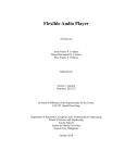
Here a zero in a particular position in FIODIR means the pin is used for input, and the relevant bit in FIOPIN
contains its current state. Writes to FIOPIN,FIOCLR or FIOSET don’t affect input pins, and making changes
to the value of an input pin is basically a no-op.
7
Figure 1: A pull-down resistor allows for more predictable
connections between logic gates and inputs. With the
resistor, when the button is released, the ground will pull
the voltage back down to 0v. Without the resistor, a
sufficiently isolated pin might stay at 3v even after the
button is released, giving an incorrect reading. Additionally,
having a large resistor is important since it will only draw
a small amount of current when the button is pressed. A
small resistor might draw enough to stress the power supply
and keep other portions of your device from functioning
GPIO Input
3v
Pull Down Resistor
100 kΩ
Button
Once you have this set up, you can connect up a switch with a pull down resistor to the input pin, and be
able to read the state of your button in software.
2.4.2
Bouncing
So if you want to toggle an LED whenever you press a button you might do something like the following.
int state, prevstate = 0;
while(1){
// Get state of P0[9]
state = (LPC_GPIO0->FIOPIN >> 9) & 1;
// If there's a change from 0 to 1
if(!prevstate && state) {
// Toggle P0[8]
LPC_GPIO0->FIOPIN ^= 1 << 8;
}
prevstate = state;
}
When you try that, you’ll notice some odd behavior, not only will the LED change when you press the
button, but it will occasionally also change when you release the button. Sometimes it’ll miss button presses
completely, and not change the LED’s state.
8
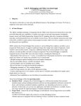
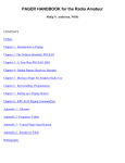
Figure 2: What button presses actually look like.
This happens because buttons aren’t perfect, and instead of getting smooth transitions from connected to
disconnected, the transitions are disjointed and shaky, this phenomenon is known as bouncing.8 Because the
GPIO pins can only read if something is low or high these jitters result in a number of very fast transitions
before the voltage stabilizes. Your LPC will see some of these transitions as a separate button presses and
toggle the LED accordingly. Most of the time, the bouncing will happen between reads of the pin state but
sometimes, a read will happen in the middle of the bouncing and cause anomalous output.
Removing the errors caused by bouncing can be done with hardware or software. In hardware, using a
capacitor or a Schmitt Trigger can sometimes solve the problem. In software, one can check if the input has
been stable for a while before acting upon an event. There are also many other ways to deal with bouncing
that can be more complex but also more reliable.
2.4.3
Interrupts
There’s another way to get input from GPIO pins, this time without having to stop and poll the state of
your button waiting for something to happen. With the correct settings the processor can wait for an event
in the background while letting your code run in the meantime. When an event occurs, the processor will
stop your currently running code, run code to respond to the event, and restart the execution of your main
program. This mode of communication is known as Interrupt Driven I/O.
These interrupts can be very complex and so we’re only going to touch on a small subset of their capabilities
here. For GPIO specifically, an interrupt can be triggered when the CPU detects a rising or falling edge9 on
an input pin. Once the edge is detected, the Interrupt Controller performs a context switch. In this case,
saving any of the current registers to the stack, and starting the executing of the interrupt handler. Once the
interrupt handler is done, the processor will restore the previously saved registers, and continue executing the
original code.
The Interrupt Controller uses an internal flag to determine whether or not to perform a context switch, and
this flag is not automatically turned off once it has been set. This means that if you don’t manually disable
the flag, the interrupt handler will execute repeatedly until the flag is disabled.
8 Image
9A
taken from http://en.wikipedia.org/wiki/File:Bouncy_Switch.png
rising edge is the pin’s value changing from a 0 to a 1, and a falling edge is the value changing from a 1 to a 0.
9
This might not seem useful, but consider a case where you’ve got a number of interrupts coming in
simultaneously. Because the flag isn’t automatically disabled, you can handle one incoming interrupt, disable
the flag for that particular interrupt, and know that the Interrupt Controller will automatically call another
handler to care of the other interrupts.
Interrupt chaining lets you keep your code small, and modular while still being able to handle many quickly
incoming events. By only disabling the flag for the particular event you’ve handled, you are guaranteed to
have your interrupt handler called again, so that it can handle a different event.
2.4.3.1 Setting Up an Interrupt Handler Setting up a GPIO interrupt starts with telling the Interrupt
Controller or NVIC 10 that you want certain pins to trigger interrupts. In the struct LPC_GPIOINT you’ll find
the registers IO0IntEnR and IO0IntEnF which define which pins on GPIO Port 0 generate interrupts on a
rising and falling edge.11
Next the specific interrupt handler must be enabled. All the GPIO interrupts are handled by External
Interrupt 3, so we’ll use a macro to tell the NVIC that it’s allowed to call that specific handler.
// Enable Rising Edge Interrupt on P0[9]
LPC_GPIOINT->IO0IntEnR |= (1 << 9);
// Enable Falling Edge Interrupt on P0[9]
LPC_GPIOINT->IO0IntEnF |= (1 << 9);
// Turn on External Interrupt 3
NVIC_EnableIRQ(EINT3_IRQn);
In order for the interrupt to do anything, the handler has to be defined. The interrupt handlers are found in
cr_startup_lpc176x.c in each of your project’s source directories, defined as weak aliases to the default
interrupt handler. Because they’re weakly defined, defining a new function with the same name will make
that the handler for the interrupt.
// Turn on the LED when the button is pressed
void EINT3_IRQHandler() {
// If the rising edge interrupt was triggered
if((LPC_GPIOINT->IO0IntStatR >> 9) & 1){
// Turn on P0[8]
LPC_GPIO0->FIOPIN |= 1 << 8;
}
// If the falling edge interrupt was triggered
if((LPC_GPIOINT->IO0IntStatF >> 9) & 1){
// Turn off P0[8]
LPC_GPIO0->FIOPIN &= ~(1 << 8);
}
// Clear the Interrupt on P0[9]
LPC_GPIOINT->IO0IntClr |= (1 << 9);
}
All the GPIO Interrupts share the same interrupt handler, so it has to check which pins actually triggered
the interrupt. You can do this with the GPIO Interrupt Status Registers. IO0IntStatR will have bits set
when the relevant pin was triggered by a rising edge, and IO0IntStatF does the same for a falling edge.
10 NVIC
: Nested Vector Interrupt Controller
registers are for pins on GPIO Port 0. There are similar registers with IO2 instead for pins on GPIO Port 2. The
other GPIO ports don’t have support for interrupts, and don’t have interrupt registers.
11 These
10
Once you’ve done the relevant action you can clear a particular pin’s interrupt flag by writing a 1 to the bit
in IO0IntClr. This means you only have to handle one pin at a time, and as long as you clear that pin’s
interrupt flag, the handler will be called again to take care of the next triggered pin.
2.5
Project : Bit Banging
Bit banging is the process of implementing a serhttp://www.cs.umd.edu/~rohit/UESDbook.pdfial communication protocol using software instead of dedicated hardware. In this case we’re going to be sending data to a
shift register, using 3 GPIO pins to control 8 LEDs.
2.5.1
Shift Registers
To control many LEDs with few outputs you need to implement a serial communications protocol, a way
of sending data one bit at a time to another entity. In this case we are going to be sending the data to a
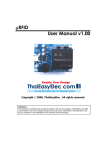
CD4094B, which has an interface based around 3 input lines, the clock, the data line, and the strobe input.
Clock
Data
Strobe
Data Bit
Shift Register
Output Value
0
0x00
0x00
1
0x01
0x00
1
0x03
0x00
0
0x06
0x00
1
0x0D
0x00
0
0x1A
0x00
0
0x34
0x00
1
0x69
0x00
x
0x69
0x69
Figure 3: Shift Register Timing Diagram
The CD4094B has, in effect12 , two registers inside of it, a shift register and an output register. The shift
register is used to load in data one bit at a time, so whenever the clock signal moves from low to high it’ll do
two things:
1. It will shift the data it contains one bit to the right.
2. Now that the lowest bit is empty, it’ll read the value on the data line and store it in that least significant
bit.
So this way, through 8 clock cycles you can load one byte onto the shift register, starting with the highest
first.
The output register is what is actually connected to the external pins, and determine whether each output
pin is held low or high. This register waits till it sees a rising edge on the strobe input, and when it does, it’ll
copy over the values currently in the shift register.
With this, you can load in a byte of data with the clock and data lines, and once you’ve finished, write it all
at once to the output with the strobe line.
2.5.2
Materials
Other than your LPC you’ll need the following:
12 Thinking of them as memory registers is an imperfect abstraction. While it’ll serve for anything we need to do, there are
much more detailed explanations on the CD4094B Data Sheet and on Wikipedia
11
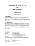
• 1 x CD4094B 8-Bit Shift Register
• 8 x LEDs
• 8 x 2N2222A NPN Transistor 13
The shift register in this circuit can channel only 10mA of current, and if you connected it directly to the
LEDs you’d get a glow that’s barely visible. The transistors act as simple current amplifiers so that you can
have brighter LEDs.
2.5.3
Steps
1. Wire up the following circuit
3v
Q5
2N2222
Q6
2N2222
Q7
2N2222
Q8
2N2222
3v
Vdd
Enable
Q5
Q6
Q7
Q8
Q's
Qs
Q3
Q4
Vss
D5
D6
D7
D8
D1
D2
D3
D4
CD4094B
8-bit Tri State
Shift Register
GPIO A
Strobe
Data
Clock
Q1
Q2
GPIO B
GPIO C
Q1
2N2222
Q2
2N2222
Q3
2N2222
Q4
2N2222
3v
Figure 4: Shift Register Circuit
2. Implement the serial protocol needed to write to shift registers, and display a pattern where one LED
turns on at a time, moving back and forth across the back of LEDs.
3. Use interrupts to detect the state of a button connected to GPIO and switch between two patterns
when it is pressed.
4. Use fast switching to make the LEDs glow at different brightnesses while displaying some pattern, and
having some interrupt based button interaction.
5. Bonus: Chain up two more shift registers, and use 8 RGB LEDs to display 3 distinct patterns, one in
each color channel. 14
13 The
14 The
2N2222A and PN2222A are functionally equivalent transistors with different packages, so feel free to use either.
shift register data sheet has a diagram showing how to chain them for more storage.
12
3
Clocking
Paragraph about clocking being a tradeoff between processing power and power consumptions, and segue into LPC stuff
Clocks in the LPC all derive from one of three oscillators.
Main Oscillator This is the usual clock source for the LPC and runs at 12MHz.
Internal RC Oscillator This is driven by an internal RC circuit at 4MHz, and is the clock the LPC uses
when it’s reset. Usually software will later switch to the Main Oscillator.
Real Time Clock (RTC) Oscillator This is a 32.768 KHz Oscillator that powers the real time clock.
Because of the precisely chosen frequency, the clock can increment a 32 bit counter on every tick, and
overflow once a second.
Each of these clocks can be used as a cpu clock, or with the help of a Phase Locked Loop (PLL) generate a
much faster CPU clock, up to the LPC’s limit of 120MHz.
Before we can get into how to set the LPC’s clock, there are two components you need to understand: Clock
Dividers, and Phase Locked Loops.
3.1
Clock Dividers
Factor Register
Input Signal
Output Signal
Edge Detector
Test
Toggle
=
Reset
Counter Register
Increment
Figure 5: Clock Divider Block Diagram
Clock Dividers are an integral part of any complex clocking system. They allow you to turn a single precisely
timed clock signal into another running an integer multiple slower.
As shown in Figure 5, internally they have two registers, a counter register, and a factor register. The counter
register simply counts all the edges in the input signal. And the factor register stores the amount by which
the input signal is slowed down, and is usually user modifiable.
During operation, there is an edge detector, which will trigger two events whenever it sees a rising or falling
edge on the input signal.
1. It will test if the value in the factor register is equal to the value of the counter register.
2. It will increment the counter register.
Then, if the equality test was successful it will perform two more actions.
3. Reset the counter register to 0.
4. Toggle the state of the output signal, switching low to high and vice versa.
13
If the number in the factor register is N , then the period of the input signal will be multiplied by N + 1 and
the frequency will be divided by the same amount, as shown in Figure 6. So, if Fin and Fout are, respectively,
in
the input and output frequencies then NF+1
= Fout
Input Signal:
Factor 0:
Output
Counter
Factor 1:
Output
Counter
Factor 4:
Output
Counter
0 0 0 0 0 0 0 0 0 0 0 0 0 0 0 0 0 0 0 0 0 0 0 0 0 0 0 0 0 0 0 0 0 0 0 0 0 0 0 0
0 1 0 1 0 1 0 1 0 1 0 1 0 1 0 1 0 1 0 1 0 1 0 1 0 1 0 1 0 1 0 1 0 1 0 1 0 1 0 1
0 1 2 3 4 0 1 2 3 4 0 1 2 3 4 0 1 2 3 4 0 1 2 3 4 0 1 2 3 4 0 1 2 3 4 0 1 2 3 4
Figure 6: Clock Divider Timing Example
3.2
Phase Locked Loops
Initial Target Frequency Approximation
Input Signal
Phase / Frequency
Comparator
Approximation
Error Term
Current Controlled Oscillator
(CCO)
+
Multiplicative
Clock Divider
(M-Divider)
Output Signal
Scaling Divider /2
(Factor = 1)
Figure 7: PLL0 Block Diagram
PLLs are clock multipliers, where a clock divider will divide the frequency of an incoming signal, a PLL will
multiply it. A PLL is a complex self correcting feedback loop, but in order to use it all one needs to know is
that Fin × 2 × (M + 1) = Fout where M is the value in the M-Divider’s factor register.15
To see how the PLL works, one must first understand that it is a feedback loop, it starts with an approximation
of the final output signal and refines it till it’s an exact multiple of the input signal.
Within the PLL is a Current Controlled Oscillator (CCO) that will generate the final output signal, it starts
oscillating at some frequency that’s close, but not quite what we want. The output of the CCO is divided by
both the Scaling Divider and the M-Divider to get an approximation for the incoming signal.
Fout
If Fapprox is the frequency of the approximated signal, we know that Fapprox = 2×(M
+1) , because the output
signal is divided twice before it becomes the approximation. If we’re lucky enough that Fapprox = Fin we can
substitute and solve to show that Fout = 2 × (M + 1) × Fin , meaning that we’ve successfully multiplied the
frequency of our input signal.
15 The equation accounts for the extra scaling divider that is in the LPC’s PLL0. A standard PLL doesn’t have this extra
divider, with the CCO being connected directly to the M-Divider, and therefore has the equation Fin × (M + 1) = Fout .
14
But if Fapprox 6= Fin then how does the PLL make Fapprox = Fin ?
Start
Error
Correction
Case 1
Input
CCO
Approximation
No Error
No Correction
Case 2
Input
CCO
Approximation
Too Fast
Slow Down CC0
Case 3
Input
CCO
Approximation
Too Slow
Speed Up CC0
Figure 8: PLL Error Correction
This is done by the Phase/Frequency Comparator which can figure out if the approximation is running at a
higher or lower frequency than the input, or if the approximation and the input have a different phase. The
difference between the approximation and the input constitute an error term. Figure 8, shows the ways the
error term can be combined with the current state of CCO to create a refined approximation.
This continual process of error checking and correction means the PLL becomes locked to the input signal,
and outputs a precisely frequency multiplied version thereof.
3.3
Calculating Clock Speed
cclk
Main Oscillator : osc_clk
Real Time Clock Oscillator : rtc_clk
sysclk
pllclk
PLL0
N-Divider
Internal RC Oscillator : irc_osc
Main PLL
(PLL0)
System Clock Select
CLKSRCSEL[1:0]
CPU Clock
Divider
pclk1
Peripheral
Clock
Dividers
pclk2
pclk4
pclk8
CPU Clock Divider Setting
CCLKCFG[7:0]
Main PLL Settings
PLL0...
CPU PLL Select
PLL0CON
Figure 9: Cpu Clock Generation Diagram
Calculating the current clock speed is a matter of following each of the intermediate steps between the three
core oscillators, and the final cclk signal that actually clocks the LPC’s CPU.
sysclk This can be connected to any of the core oscillators on the LPC, so its frequency can be 12MHz if
connected to osc_clk, 4MHz if connected to irc_osc or 32.7 KHz if connected to irc_osc.
pll0clk This is the output of PLL0, and its frequency must be between 275 MHz and 550MHz.
If you let,
15
N = The value in the PLL0 N-Divider’s factor register
M = The value in the PLL0 internal clock divider’s factor register
then
Fpll0clk =
2 × (M + 1) × Fsysclk
N +1
pllclk This is the output of the CPU PLL Selector and can be set to either sysclk or pll0clk,
cclk This is your final system clock, and is pllclk divided by the CPU Clock Divider, this can be at most
120 MHz.
If you let
D = The value in the CPU Clock Divider’s Factor Register
then
Fcclk =
3.4
Fpllclk
D+1
Working Backwards
If we want to change our LPC’s clock speed, we must answer the following questions:
• Which oscillator should be connected to sysclk?
• Should we use the PLL, and if so what should the N-Divider, and M-Divider be set to?
• What should the CPU Clock Divider be set to?
We also must keep in mind the following restrictions:
• The CPU factor register on supports values between 0 and 255.
• The N-Divider’s factor register only supports values between 1 and 32
• The M-Divider’s factor register only supports values between 6 and 512 and a number of extra values
seen on page 38 in the manual.
• If we’re using PLL0 it must output a signal between 275MHz and 550MHz.
• The final clock speed cannot be more than 120MHz.
In order to figure out all of the above we should work backwards from our target cclk frequency, Fcclk .
First, we should check if we can forgo the PLL entirely. For every oscillator check if Fcclk ≤ Foscillator . If it
is, check if Foscillator
is an integer less than 256. If that too is true, then we can do the following:
Fcclk
1) Set sysclk to connect to that oscillator.
2) Bypass PLL0, connecting sysclk directly to pllclk.
3) And set the CPU Clock Divider to Foscillator
− 1.
Fcclk
16
If we couldn’t forgo the PLL, then we need to figure out the PLL settings we’ll use. If we’re using PLL0, we
know Fpllclk is less than 275MHz, and 550MHz, and that for some integer D between 0 and 255:
Fpllclk = (D + 1) × Fcclk
The PLL consumes less power when it runs at a lower frequency, so we should choose the smallest D that will
fit within the bounds.
Now we know we’ve got to set the CPU Clock Divider to D, but we still have to figure out which oscillator
to use, and what to set the N and M dividers to.
We want this to be true:
Fpllclk =
2 × (M + 1) × Fsysclk
N +1
We can solve and substitute to get:
N +1
2 × Foscillator
≈
M +1
Fpllclk
So for each oscillator we can find the best approximation for the right hand side possible using a valid N and
M . Namely with N between 1 and 32, and M between 6 and 512 (or another value given on page 38 of the
manual). We can then choose which combination of oscillator, N and M will give us the least error.
Namely if we let
2 × Foscillator
Fpllclk
δ = The error for any combination of oscillator, N and M .
R=
then
δ=
N +1
M +1
−R
!2
R
Once we have the settings that’ll minimize the timing error, we can do the following:
1)
2)
3)
4)
3.5
Set sysclk to the proper oscillator.
Set the N-Divider and M-Divider to N and M , respectively.
Connect PLL0 to pllclk.
And set the CPU Clock Divider to D.
Making The Changes
Now that we know how to choose the various clocking settings we’ll use, we need to learn how to apply them.
This involves making absolutely sure that you perform certain operations in a certain order, checking and
double checking the state of the system, and operations that serve only to prove to the LPC you’re paying
attention.
Clocking can be a dangerous subsystem to play around in, if we input badly chosen settings, we could render
our microcontrollers useless. This is why the LPC’s clocking subsystem requires people to jump through
hoops to change anything.
17
3.5.1
Registers
Before we dive into the algorithm to change the settings, we should step through the various registers we’ll
be using and look at their functions.
LPC_SC->CLKSRCSEL The Clock Source selection register, this is what will connect a particular oscillator to
sysclk. Look at page 34 of the manual for more details on how to operate it.
LPC_SC->CCLKCFG The CPU Clock Divider’s factor register, this controls the divider placed right before
CCLK. See manual page 54.
LPC_SC->PLL0STAT The PLL0 Status register, this read-only register makes the currently applied PLL0
settings visible to you. It has the connection status of PLL0 the N-Divider and M-Divider factor
registers, and a status bit which tells you if the PLL is synced yet with its input signal. See manual
page 39.
LPC_SC->PLL0CON The PLL0 Control register, this register controls whether PLL0 is on, and lets you choose
between connecting pllclk directly to sysclk or to PLL0 See manual page 37.
LPC_SC->PLL0CFG The PLL0 Configuration register, this is where you set the factor registers for the N-Divider
and M-Divider. See manual page 37.
LPC_SC->PLL0FEED The PLL0 Feed register, you write afeed sequence to this register in quick succession in
order to validate changes you’ve made to the other PLL0 registers, and actually apply them to the
PLL. See manual page 40.
3.5.2
Feed Sequence
The PLL registers together form an update-commit system, where every change of PLL settings requires a
feed sequence in order to actually be applied. This exists so that random memory accesses won’t change the
settings on this device, and if you want to break your LPC you’ve got to actually work to do it.
A feed sequence consists of writing 0xAA and 0x55 to PLL0FEED one after the other, with no other memory
operations on any of the other system control registers in between.
void PLL0_feed_sequence(){
LPC_SC->PLLOFEED = 0xAA;
LPC_SC->PLLOFEED = 0x55;
}
3.5.3
Update Algorithm
When you have chosen your settings, there’s a well specified algorithm 16 which explains what changes you
have to make and in what order. It is very important that you don’t combine steps, and make sure that you
get no interrupts during this process.
1) Check if PLL0 is already connected, if it is disable it with one feed sequence.17
16 See
17 See
page 46 in the manual
the appendix for all the macros used herein
18
if(GETBIT(LPC_SC->PLL0STAT,25)){ // If PLL0 is connected
BITOFF(LPC_SC->PLL0CON,1);
// Write disconnect flag
PLL0_feed_sequence();
// Commit changes
}
2) Disable PLL0 with a feed sequence.
BITOFF(LPC_SC->PLL0CON,0);
PLL0_feed_sequence();
// Write disable flag
// Commit changes
3) If you do not plan to use the PLL, set the CPU clock divider to your final value, otherwise set it to 1.
// Change CPU Divider
LPC_SC->CCLKSEL = <CPU Clock Divider Value>;
4) Write to the Clock Source Selection Control register to change the clock source if needed.
// Change sysclk source
LPC_SC->CLKSRCSEL = <Clock Identifier Bits>;
5) If you are not using the PLL, you are done, otherwise continue.
6) Write values to the N-Divider and M-Divider and use a feed sequence to enable them. The dividers can
only be updated when PLL0 is disabled.
// Write divider values
SETBITS(LPC_SC->PLL0CFG,0,14,<M-Divider Value>);
SETBITS(LPC_SC->PLL0CFG,23,16,<N-Divider Value>);
PLL0_feed_sequence(); // Commit Changes
7) Enable PLL0 with one feed sequence.
BITON(LPC_SC->PLL0CON,0); // Set Enable Flag
PLL0_feed_sequence(); // Commit Changes
8) Set the CPU Clock Divider to its final value. It is critical to do this before connecting PLL0.
LPC_SC->CCLKSEL = <CPU Clock Divider Value>; // Change Clock Divider
9) Wait for PLL0 to achieve lock.
Let
Fpllref =
If 100kHz ≤ Fpllref ≤ 20MHz wait for the PLL to lock.
19
Fsysclk
N +1
while(! GETBIT(LPC_SC->PLL0STAT,26)); // Spin on Lock Flag
If Fpllref < 100kHz wait for 200/Fpllref seconds.
int i,count = <Number of cycles with current clock speed>;
while(i++ < count); // Wait sensible amount of time
If 20MHz < Fpllref wait for 200µs.
int i,count = <Number of cycles with current clock speed>;
while(i++ < count); // Wait sensible amount of time
10) Connect PLL0 with a feed sequence.
BITON(LPC_SC->PLL0CON,1); //Set PLL0 Connect Flag
PLL0_feed_sequence(); // Commit Changes
3.6
Peripheral Clocks
Many peripherals are timed using the Peripheral Clock Dividers. There are four clocks pclk1,pclk2,pclk4
and pclk8, which are clocks derived from cclk, and are 1,2,4,and 8 times as slow as cclk. Namely, they are
implemented with clock dividers with fixed factor registers of 0,1,3 and 7.
You can see how to connect them to various paripherals on pages 56 and 57 of the manual.
3.7
Project : Precision Timing
Many aspects of your LPC require very precise clocking. Things like the USB subsystem, the Analog to
Digital Converter (ADC) and Direct Memory Access (DMA) all perform operations that are timed using your
internal CPU clock. The accuracy of those features, and more depends on how accurate your clock speed is.
We are going to experiment with changing the clock speed to generate output signals at various frequencies.
3.7.1
Steps
1) Write a script, in any laguage you want, that will calculate clock settings for you. It should, given a
target clock speed, give you everything needed to write the clock setup code.
$ ./clk-calc --target=120MHz
Base Oscillator : ...
Use PLL : ...
N-Divider : ...
M-Divider : ...
CPU Clock Divider : ...
Target Freq: ...
Output Freq: ...
20
Error: ...
$ ./clk-calc --target=200MHz
Cannot Compute: Target Clock Too High
2) Write a program that repeatedly toggles a GPIO pin, so that you get a square wave.
3) Use make lst and the ARM Cortex M3 Manual to find the number of clock cycles between every
toggle.
4) Change the frequency of your output square wave without changing the loop at all, use only different
clocking settings.
3.7.2
Questions
As you progress through the exercise, answer the followign questions:
1) What is the lowest CPU clock speed you can achieve with this setup?
2) How many clock cycles does your loop take between GPIO toggles?
3) What are the options needed to get the maximum speed, 120MHz?
4) What is the frequency of your output signal when the CPU clock is 200Hz? 120MHz?
5) What clock frequency do you need to get an output signal at 1kHz?
21
4
Timers
Intro Paragraph for Timers, something about real time systems?
4.1
Basic Description
Timers are peripherals within the LPC that are mainly internal, they use the CPU clock to keep track of
time, and make that ability available to the user in a number of ways.
Timers can send out periodic events, make very precise measurements, simply make the time available for
your applications, among other things. This means you can start using temporal information in your program,
without having to use unwieldy spin loops, and other ill advised hacks.
There are four timers within the LPC, Tim0, Tim1, Tim2 and Tim3. All are identical, but can have options
set independently, and can be used without interfering with each other. ‘
4.2
Speed Settings
pclk1
pclk2
Prescaling
Clock Divider
pclk4
pclk8
Prescale Counter
LPC_TIMx->PC
Peripheral Clock Selector
PCLKSELx
Increment
on
Toggle
Timer Counter
Reset? Disable?
Timer Control
Register
Figure 10: Timer Counter Block Diagram
All timers are built around an internal Timer Counter (TC), which is a 32 bit register that is incremented
periodically. The rate of change is derived from the current speed of the CPU clock, which peripheral clock
you’ve connected up and what the prescale counter is set to.
There’s nothing more to it than that, the prescale counter is a clock divider like so many others, and the
Timer counter is a 32 bit register, and as long as nothing else intervenes it’s count from 0x00000000 to
0xFFFFFFFF, overflow, and do it all over again.
4.2.1
Powering Devices
Before we can get to choosing the peripheral clock, and setting the prescale register, we need to actually tun
on the timer.
On reset most of the LPC’s peripherals are off, and aren’t being supplied power by the microcontroller. This
can save a lot of energy, but a few core peripherals are turned on when the LPC starts, among these GPIO
and Tim0 and Tim1. But this means that Tim2 and Tim3 start off, and if you need them you’ll have to turn
them on. Additionally, if you don’t need Tim0 or Tim1, you can turn them off to save some power.
Power control is considered a system feature, and is controlled by register LPC_SC->PCONP. Each bit in that
register is assigned to a peripheral, with a 0 meaning unpowered, and a 1 meaning that the peripheral is
powered.
22
BITON(LPC_SC->PCONP,22); // Turn on Tim2
BITOFF(LPC_SC->PCONP,2); // Turn off Tim1
You can find the full table of peripheral to bit mappings on pages 63 and 64 of the manual.
It’s probably a good idea to note that you can get some very weird results if you try to work with a peripheral
that’s off. The whole situation has undefined results, but in practice, writes to registers in unpowered
peripherals don’t do anything, and reads always return 0.
4.2.2
Choosing a Peripheral Clock
Likewise, choosing a peripheral clock is a system function, and the settings for all the peripherals are on
LPC_SC->PCLKSEL0 and LPC_SC->PCLKSEL1.
SETBITS(LPC_SC->PCLKSEL0,4,2,0b10); // Set Tim1 to use pclk2
SETBITS(LPC_SC->PCLKSEL1,14,2,0b00); // Set Tim3 to use pclk4
You can find the bit assignments, and settings for the peripheral clock selection on pages 56 and 57 of the
manual.18
4.2.3
Setting the Prescale Counter
Once you’ve made sure your chosen timer is on, and is using the peripheral clock you want, you can move
onto setting the prescale counter and actually using it to perform timing related tasks.
The prescale counter is basically a 32 bit factor register inside a clock divider. You can set it using the
LPC_TIMx->PC register.
LPC_TIM3->PC = 14; // Divide the incoming clock by 15.
All of this can be found on page 495 of the manual.
4.2.4
Reset and Enable
Before the timer counter can actually start incrementing, there are two flags within the Timer Control
Register (TCR).
The enable flag, when set to one, disables the timer counter’s ability to increment.
BITON(LPC_TIM2->TCR,0); // Disable the timer counter
BITOFF(LPC_TIM2->TCR,0); // Enable the timer counter
The reset flag, when set to one, forces the timer counter’s value to zero.
18 The
choice of bits to select each clock is somewhat odd, so do look at the manual
23
BITON(LPC_TIM0->TCR,0); // Disable the timer counter
// The couter's value is stuck wherever we stopped it
BITON(LPC_TIM0->TCR,1); // Reset the timer counter to zero
// The counter's value is zero
BITOFF(LPC_TIM0->TCR,0); // Enable the timer counter
// The counter's value is *still* zero, since the reset bit is still on
BITOFF(LPC_TIM0->TCR,1); // Disable the reset flag
// The counter's value will now start incrementing, since the
//
reset flag is gone.
Once you’re done with setting those value properly, you can watch your timer counter increment.
Current_Timer_Val = LPC_TIM3->TC;
4.3
Match Registers
Match Register
Match Control
Register
Disable?
Timer Counter
=
Reset?
Interrupt?
Reset? Disable?
Timer Control
Register
Disable
Interrupt
Reset
Figure 11: Match Register Block Diagram
Within each timer are four match registers, 32 bit registers which can store a specific match value. When the
timer counter and match register are equal, certain events can be triggered.
Choosing the match value is just a matter of setting the match register, LPC_TIMx->MRx.
LPC_TIM0->MR3 = (uint32_t) 4000; // Set match register 3 on timer 0
LPC_TIM2->MR1 = (uint32_t) 453; // Set match register 1 on timer 2
4.3.1
Match Settings
There are three events a match can trigger, a reset of the timer counter, disabling the timer counter and
sending an interrupt. The disable and reset events work by modifying the timer control register, and using
its features to control the timer counter.
24
The match register’s disable event sets the disable flag in the TCR to 1, requiring you to manually toggle it
back. On the other hand, the reset event simply toggles the flag in the TCR, setting the timer counter to 0,
but allowing it to continue incrementing,
Insert timing diagrams showing outcome of disable and reset flags
To actually change which events are triggered on match requires manipulating the register at LPC_TIMx->MCR.
All the flags for all the timer registers are mapped to various bits in the Match Control Register (MCR). This
mapping can be found on page 496 on the manual.
BITON(LPC_TIM0->MCR,10); //
//
BOTON(LPC_TIM2->MCR,5); //
//
4.3.2
Reset on match for
match register 3 in timer 0
Disable on match for
match register 3 in timer 2
Match Interrupts
Like a GPIO interrupt, there are multiple triggers which all trigger an interrupt on the same channet. Each
of the match registers can trigger interrupts, and so can other components of each timer.
To tell these interrupts apart, you can use each timer’s Interrupt Register (IR). When a component of the
timer triggers the interrupt a flag in the IR is flipped and you can use that to determine what’s already going
on.
4.3.3
External Match Registers
Explanation of how external pins can be modified by match output without CPU intervention.
4.4
Capture Registers
Capture Control
Register
Enable?
Enable?
Interrupt?
TIMERx IRQ
CAPn.x Pin
Timer Counter
Load
Capture Register
Figure 12: Capture Register Block Diagram
Explanation of capture register structure and function with example code
25
Explain: Interrupt
channel or make
sure it’s used earlier
4.5
Project : Serial Light Communications
Explanation of project.
4.5.1
Background
Missing
figure
Oscilloscope readout
explain rise/fall time, timing and synchronization considerations
4.5.2
•
•
•
•
•
4.5.3
Materials
1
1
1
1
1
x
x
x
x
x
LED (use the bright blue ones on the strip)
Photoresistor
Potentiometer
2kOhm Resistor
TLV2461 Op-Amp
Steps
GPIO Out
LED
Figure 13: LED Output Circuit
26
3v
PR1
P1
GPIO In
TLV2461
R1
2 kΩ
Figure 14: Light Recieve Circuit
Explain voltage dividers and the maths behind it
27
5
ADC
Intro Paragraph
The ADC is the analog counterpart to the GPIO’s input mode. There are 8 ADC channels each of which can
read in a single value at a time.
5.1
Theory of Operation
Explain how the ADC works, what is meant by ’bits of precision’ and the mapping from D->A->D.
5.2
Basic Usage
Explain how to read a single value from the ADC, setting it up, waiting for the done bit, setting the clock, etc.
Explain how the ADC takes 65 clock cycles to pin down a value, how the various status registers interact.
Explain the various settings in the control register, the structure and mapping between the global data register and the various channel specific data
registers, and the status register. the trim register can be ignored for the moment, and the interrupt register we’ll handle in that section
The initial setup of the ADC consists of the following steps:
1) Power the device
Here we set the bit in LPC_SC->PCONP for the ADC, to turn the power on. This is essentially the same as for
the Timers and most other peripherals.
LPC_SC->PCONP |= 1 << 12; // Manual page 56-57
2) Calculate the necessary clock (the ADC can only run at 13MHz) and choose a peripheral clock, and
ADC clock divider setting.
The ADC, like most other components is connected to your choice of peripheral clock and then run through
its own divider. The ADC is also limited to a 13 MHZ clock, so you must choose values for its internal clock
divider, and peripheral clock such that
Fpclkx
< 13MHz
N +1
The easiest way to do this is to simply set your central clock to the 12MHz main oscillator, and the various
other dividers to pass that through unchanged.
LPC_SC ->CLKSRCSEL = 1;
LPC_SC ->PLL0CON = 0;
// Select main clock source
// Bypass PLL0, use clock source directly
// Feed the PLL register so the PLL0CON value goes into effect
LPC_SC ->PLL0FEED = 0xAA; // set to 0xAA
LPC_SC ->PLL0FEED = 0x55; // set to 0x55
// Set clock divider to 0 + 1=1
LPC_SC ->CCLKCFG = 0;
28
Comment [ROHIT1]: This is uncomfortably like a
cookbook one can
follow blindly
But you can also use settings that will let your LPC run faster, and get more out the main processor while
allowing the ADC to run as fast as possible,
3) Set the peripheral clock
Here we use the undivided clock for the ADC, but as long as the final clock constraints are considered, you
can choose any peripheral clock.
// Choose undivided peripheral clock for ADC
LPC_SC->PCLKSEL0 &= ~(3 << 24);
LPC_SC->PCLKSEL0 |= (1 << 24);
4) Set the ADC clock divider
The ADC control register, LPC_ADC->ADCR controls a number of functions, but for the moment we’ll use it to
choose the setting for the ADC clock divider. This is controlled by bits 8 through 16 of the control register
and can be set as follows.
SETBITS(LPC_ADC->ADCR,8,8,0); // Set clock divider to let the
// clock pass unchanged
5) Put the pins you’ll be using into ADC mode
SETBITS(LPC_PINCON->PINSEL1,14,2,0b01); // Connect AD0.0 to its pin
6) Pull the ADC out of power down mode
The ADC also has its own internal power switch, so that you can change settings while conserving power
that the conversion circuitry will use.
BITON(LPC_ADC->ADCR,21); // Turn on ADC internal power
The simplest method of actually getting data is synchronous collection of values from the ADC. You tell the
ADC to go collect some data, wait for it to tell you it’s done, and then read out the value.
When trying to synchronously access one of the eight ADC lines, do the following:
1) Select the ADC line you’re going to read.
The first eight bits in LPC_ADC->ADCR control which input lines are active, and when collecting data
synchronously, you can only have one on at a time.
LPC_ADC->ADCR &= 0xFF; // Clear first 8 lines
BITON(LPC_ADC->ADCR,0); // Choose line 0
2) Start the conversion
There are 3 bits in the ADC control register which let you choose the collection mode, for the moment we’ll
focus on the first two. Setting bits 24 to 26 in the ADCR to 0 tells the ADC that you want no conversion done,
and setting them to 1 tell the ADC to start a conversion immediately.
29
SETBITS(LPC_ADC->ADCR,24,3,1); // Start the single conversion
3) Spin on the done flag
For single conversions you can look at the General Data Register which will store the results of the very last
conversion. Because a conversion takes 65 of the ADC’s clock cycles, where it’ll spend time slowly increasing
the precision of the value it recovers, you have to wait for it to finish. So you spin on the done flag in the
final bit of the data register, which will turn to 1 when the conversion is finally finished.
while((LPC_ADC->ADGDR & (1 << 31)) == 0);
4) Read and parse the output value
And now you can find your converted value in the same register, in bits 5 through 12.
value = GETBITS(LPC_ADC->ADGDR,5,12);
5.3
Interrupts
Explain how to use the ADC interrupt, when it’s thrown, what you need to flip, and how to get periodic ADC interrupts
If you want to sample asynchronously, using interrupts you can allow your other code to run during the
relatively long sampling process.
The setup for interrupt based ADC use has a few extra steps:
1) Enabling the ADC interrupt in the NVIC.
NVIC_EnableIRQ(ADC_IRQn);
2) Setting the correct bits in the ADC Interrupt Enable register.
BITON(LPC_ADC->ADINTEN,0);
3) Setting up the interrupt handler that will retrieve your value.
Reading from the GDR will turn off the interrupt flag so you don’t have to do it manually.
void ADC_IRQHandler(void) {
/** other stuff **/
// Equivalent to above:
analog_val = (LPC_ADC ->ADGDR >> 4) & 0x0fff;
/** other stuff **/
}
Then you can start a conversion the same way as before.
30
SETBITS(LPC_ADC->ADCR,24,3,1); // Start the single conversion
65 ADC clock cycles after you do, the interrupt will be thrown and you can retrieve the value.
5.4
Connecting to Timers
Explain how to connect to a timer, trigger on match registers, capture registers, how to use a match interrupt to trigger an ADC interrupt and then get a
value while your main loop is chugging along doing its thing.
5.5
Burst Mode
Explain what burst mode is and how to use it.
5.6
DMA
Write when we get to the DMA chapter
5.7
Project : Optical Theramin
Missing
figure
Image of theramin/ someone playing a theramin
A Theramin is a Russian musical instrument, invented in 1919, and is one of the few instruments played
without ever being touched. There are two large antennas on a theramin, which can detect the approximate
position of a musician’s hands, and uses that to modulate the sound it produces. One hand is used to control
the pitch, and the other is used to control the volume.
In a standard theramin the detection works by using its antennas and the hands of the artist as opposing
plates in a capacitor. By moving their hands around the artist can change the capacitance, and the instrument
can use that change to generate different sounds.
31
Insert link to
YouTube video of
theramin?
LED
Photoresistor
LED
No Hand
No Reflected Light
Photoresistor
Nearby Hand
Light Reflected
Figure 15: Hand Sensor
Our version will work of a slightly different principle, we’ll use light to sense the distance between the hand
and our sensor. We’ll place an LED below a photo resistor, so that when there’s no hand or other obstacle,
the light from the LED will just shine onto the insensitive read of the photoresistor. But when we place our
hands above the sensor, the light from the LED will reflect back onto the sensitive portion of the photoresistor
and give us something we can sense. The farther away the hand is, the less light will be reflected back, so
this setup will give us an approximate measure of distance. We can use those measurements to modulate the
output of our DAC which will be plugged into a speaker, giving us a simple optical theramin to play with.
5.7.1
Background
5.7.1.1 Voltage Dividers Voltage Dividers are an essential part of the circuitry for our theramin, and
in order to understand how it all works, you must understand how these components work.
V++
R1
Vdiv
R2
V--
Figure 16: Voltage Divider Schematic
A standard voltage diver circuit is made with two resistors placed in series, the voltage at Vdiv is the weighted
average of the voltages at V++ and V−− .
Vdiv = (V++ − V−− )
R1
+ V−−
R1 + R2
Work through a few examples of voltage divider calculations, explain how this only applies when there’s little to no load.
##### Potentiometers #####
32
V++
Vdiv
P1
V--
Figure 17: Potentiometer Divider Schematic
Potentiometers are a special type of voltage divider which you can adjust on the fly. A potentiometer is
essentially a long resistor, where you can move Vdiv up and down along it. As such, R1 + R2 is always going
to be constant and the voltage at VDiv depends on the position of the potentiometer’s dial. The actual value
can go all the way from V++ , to V−− since you can lower either R1 or R2 down to 0.
Diagram of the internals of an actual potentiometer and an explanation of the physical devices.
Missing
figure
5.7.1.1.1
Image of photoresistor circuit
Photoresistors
Explain photoresistors and math for finding optimal resistance values
5.7.1.1.2
RC-Filters
Expand the following
• Signals having frequency components
• DAC producing impure signals because of the difference between transition time and rest time.
• Need to remove the high frequency components so that we only preserve the frequency we want to
output
33
3v
In +
In -
Vout
1.5v
TLV2461
R1
Figure 18: Op-Amp Schematic
5.7.1.2 Op-Amps Operational Amplifiers (Op-Amps) are some of the most powerful standard circuit
components. They are circuits that run an extremely simple algorithm that can be leveraged in very powerful
ways.
The Op-Amps can either push or pull current through their output, and thanks to Ohm’s law V = IR this
means that they can control the voltage at their output as well.
In figure 18 the Op-Amp is connected through a resistor to a voltage source. Depending in the state of its
inputs it can choose to do one of three things. First among these is to prevent the flow of current either in or
out, in this case there will be no current flowing cross the resistor and the voltage at Vout will be 1.5v.
Next it could push current outwards, meaning there’ll be a current flowing from the output to the 1.5 volt
source. Because of Ohm’s law, the voltage at the output will increase, if the resistor is large, the voltage will
increase very quickly, until it hits the limit of 3 volts imposed by the Op-Amp’s power source. Alternatively
if the resistor is very small, it’ll take a lot of current to increase the voltage a small amount, to the point that
the power source simply can’t supply more current. If that happens the voltage at the output will hover at
whatever value the current available can sustain.
Op-Amp modulate their output voltage with a simple algorithm. If their two inputs are held at the same
voltage, the Op-Amp will keep the output stable. If Vin+ > Vin− then the Op-Amp will raise the voltage at
its output, and if Vin+ < Vin− then the Op-Amp will lower the voltage.
This property can be exploited to create a number of useful circuits.
Input
Output
TLV2461
Figure 19: Op-Amp Voltage Follower Schematic
34
5.7.1.2.1 Op-Amp Voltage Follower An Op-Amp voltage follower has a simple function, basically it
makes sure that the output voltage is always equal to the input voltage. To understand how this is useful
we’ve got to first understand how loads can change the voltages at a point.
3v
3v
R1
3v
R1
V1
R1
V2
V3
V4
TLV2461
R2
Divider
R2
Rl
R2
Divider With Load
Rl
Voltage Follower with Load
Figure 20: Load Voltage Schematic
In figure 20, we’ve set up two voltage dividers, using the same R1 and 2 but the second divider has an extra
load resistor applied to it. V1 will be the same value as before, but because of the existence of the additional
load resistor, V2 will be a different, higher, voltage.
If, instead of connecting the load resistor directly to your divider, you connected the divider to the voltage
follower’s input, and the load resistor to the output, as with the third setup, the voltages at V1 , V3 and V4
will all be equal. Here the Op-Amp is compensating for the change in voltage the load would otherwise cause.
What is happening is that when Vin+ > Vin− the Op-Amp will increase the voltage at the output, and that
will (being directly connected) increase the voltage at Vin− . When the opposite is true and Vin+ < Vin− the
Op-Amp will decrease the voltage at output, and Vin− . Both of those actions will correct the imbalance, and
make Vin+ = Vin− and therefore Vin+ = Vout . The Op-Amp will automatically sense changes in the load,
and compensate so that the output is always equal to the input.
Input 1
Output
TLV2461
Input 2
Figure 21: Op-Amp Voltage Comparator Schematic
5.7.1.2.2 Op-Amp Voltage Comparator This is very similar to the Voltage Follower, but where the
voltage follower has a feedback loop, this circuit has no connection at all. This means that when Vin+ > Vin−
the output voltage will keep on going up till it hits the maximum voltage the Op-Amp can sustain, in our
case usually 3v. Likewise when Vin+ < Vin− the voltage will go down until it hits the lower limit, namely 0v.
So the output is limited to 0 and 3v, and its state will tell whether Vin+ > Vin− or not, comparing the two
input values.
35
R2
R1
Reference
Output
TLV2461
Input
Figure 22: Op-Amp Voltage Amplifier Schematic
5.7.1.2.3 Op-Amp Voltage Amplifier The amplifier is based off the same principle, but instead of
a direct connection, it uses a voltage divider. The voltage divider formula tells us that the, voltage at
2
Vin− = (Vout − Vref ) R1R+R
+ Vref .
2
Thanks to it’s nature as a feedback loop, the Op-Amp will change Vout so that Vin− = Vin+ . If we assume
that Vref = 0v, then we can solve the equation for Vout and see the following holds:
Vout = Vin+
R1 + R2
R2
2
So, Vout is a straightforward multiple of Vin+ , and the amount by which it is multiplied, R1R+R
is the gain
2
of the amplifier. You can do the same thing for other values of Vref to see that it’s esentially the midpoint
around which you’re multiplying. So if Vin+ = Vref + 2v then Vout = Vref + gain · 2v.
5.7.2
•
•
•
•
•
•
•
•
•
5.7.3
Materials
2
2
2
1
2
1
1
1
2
x
x
x
x
x
x
x
x
x
LED (use the bright blue ones on the strip)
Photoresistor
2 kOhm Resistor
22 Ohm Resistor
10 kOhm Resistor
Speaker
1 Microfarad Capacitor
Potentiometer (Higher Resistance is better)
TLV2461 Op-Amp
Steps
1) Build 2 Hand Sensors, test with oscilloscope.
3v
3v
PR1
ADC In
D1
R1
2 kΩ
Figure 23: Hand Sensor Circuit
36
These are voltage dividers which will use the changing resistance of the photoresistor to change the voltage at
the ADC input. Once the circuit is assembled connect the oscilloscope probe to the ADC input and wave
your hand above the sensor to get something like figure ??.
2) Connect the hand sensors to your LPC and check if you can receive ADC values with GDB or
semi-hosting.
3) Get DAC to output sin waves, verify with oscilloscope.
Once you connect your DAC output to the oscilloscope, you should see something like figure 24.
Figure 24: DAC Sine Wave Oscilliscope Trace
4) Build Voltage Reference
3v
R1
100 kΩ
Vref
TLV2461
R2
100 kΩ
Figure 25: Voltage Reference Circuit
Since your DAC is limited to values between 0 and 3 volts, we can’t amplify the output around 0v, so we’re
constructing a reference voltage for the amplifier. First we use a voltage divider to get a point at 1.5v and
then a voltage follower so that we can attach loads to that point, and have it stay stable.
Once you’ve constructed this section of the circuit, use the oscilloscope or multimeter to check that the
voltage at Vref is 1.5.
5) Build RC Filter
37
DAC
R4
22 Ω
Vsmooth
C1
1 µF
Figure 26: RC Filter Schematic
The RC filter is a component we use to smooth out the jagged edges of the DAC output. At high frequencies
the output of your DAC will look like figure 27 , with an obvious step from one output voltage value to
another. When you play this sound you’ll be able to hear the high frequency shifts as a seperate tone from
the sine wave you’re otherwise playing.
Figure 27: High Frequency DAC Sine Wave Oscilliscope Trace
To fix this you can build an RC filter, this circuit will smooth out the wave by forcing it to pour energy into
the capacitor and slowing the change in voltage. The exact workings of the filter are outside the scope of this
book, but suffice to say that it, when connected, will transform the raw DAC output in figure ?? into the
signal seen in figure 28, where the signal in yellow is the DAC after it’s connected, and the signal in pink is
the voltage at Vsmooth .
Figure 28: High Frequency RC Filter Oscilliscope Trace
6) Build Amplifier
38
Vref
R3
Vspeaker
Vsmooth
TLV2461
Figure 29: Speaker Amplifier Circuit
We can use the amplifier to change the volume of the final sound, and the amount of current the Op-Amp
will supply.
If you connect up the oscilloscope now (before adding the speaker), and have your DAC output a sine wave,
you should be able to modulate output to any gain between 1 and infinity, effectively turning the amp from a
voltage follower to a voltage comparator and anywhere in between.
Sample traces are shown in figures 30 and 31, with Vsmooth in pink, Vref in green, and Vspeaker in blue.
Figure 30: Speaker Amplifier with Small Gain
Figure 31: Speaker Amplifier Acting As Comparator
7) Connect Speaker Circuit
39
3v
R1
100 kΩ
TLV2461
R2
100 kΩ
R3
SPKR
TLV2461
C1
1 µF
R4
22 Ω
DAC
Figure 32: Speaker Circuit
Connect up your speaker to the other circuit components, and play some sound.
8) Add Calibration Routines and Basic IO
In order to actively use the theramin you’ll have to set up a calibration routine.
The amount of light on the photo-sensors, and therefore the voltage coming into your ADCs can vary wildly
depending on the brightness of the room, the relative position of your sensors and LEDs and a number of
other environmental factors. So in order to actually play your theramin you’ll have to set up a routine to tell
your LPC what range of inputs it should expect in the current environment.
This means you’ll have to set up a routine where you tell the LPC to record the maximum and minimum
voltages for each hand, and scale the output frequency and amplitude accordingly.
9) Bonus: Play something recognizable with your newly created instrument.
40
6
DAC
Intro Paragraph
The DAC is the analog counterpart to GPIO’s digital output. Your LPC has one output line, and
6.1
Working Theory
How does the DAC work, nyquist sampling, frequency? also rename this section
6.2
Usage
To set up the DAC one has to connect a particular peripheral clock to the DAC and connect the DAC output
to the corrent pin.
LPC_SC->PCLKSEL0 |= (1 << 22); // Set pclk to 1
LPC_PINCON->PINSEL1 |= 1 << 21; // Set H[18] to AOUT
To use the DAC one has to write to the DAC converter register.
SETBITS(LPC_DAC->DACR.6,10,1035); // Set DAC to 1035
41
7
DMA
Finish the intro
Often, when building embedded devices you’ll have to deal with large amounts of incoming and outgoing
data. Be it reading thousands of samples per second from the ADC as you record sound, reading megabytes
per second external memory, or sending large chunks of data over Ethernet quickly.
The simplest way to deal with these large data streams is using the CPU. Loop or timer based mechanisms
can move large amounts of data back and forth but at the cost of using CPU time to perform routine
memcopy style tasks. Occasionally it’s simply not passible to handle data at full speed, or satisfy IO timing
requirements using the CPU, and other methods are needed.
This is where Direct Memory Access (DMA) comes in, DMA is a special deeply integrated peripheral that
can perform memory manipulation tasks independent of the CPU. This means that it’s possible to perform
routine data gathering tasks faster than the CPU could, without wasting CPU time, and with a level of
timing precision that the CPU can’t match.
Missing
figure
ARM-M3 block diagram and/or DMA block diagram
The most basic use of DMA is a memory-to-memory transfer, which will copy data from one block of memory
to another. This is analogous to a standard memcpy operation, albeit without blocking. One can also choose
to have an interrupt thrown when the copy is completed in order to avoid race conditions.
The next two uses for the DMA controller are memory-to-peripheral tranfers, and peripheral to memory
transfers. These data transfers are deeply integrated with the revelant peripherals, and can be used to
automatically gather data from an input, or automatically send data to an output.
Consider the output case, where we have a buffer of data we wish to write out to the DAC at specifically
timed intervals. The DAC has a programmable countdown timer, which can ask the DMA controller for a
new piece of data after an interval. When the DAC timer finishes and a DMA request is sent, the DMA
controller will write a word into the DAC output register, and trigger an automatic outut update. At this
point, the DAC will reset the timer, and start counting down to another update, and the DMA controller will
ready the next byte of data for the DAC. In this way you can fill a buffer with sound data, and write it out
at the same rate it was recorded.
Missing
figure
DAC DMA Diagram?
42
For the input case we can look at the ADC. Like the DAC, the ADC has a timer, which can trigger a
conversion, and then assert a DMA request when it’s done. Here, when the ADC timer counts down, it’ll
immidiately start a conversion, and reset itself. When the conversion finishes, the DMA controller will read
the ADC input register, and store returned data in the predefined output buffer.
Missing
figure
ADC DMA Diagram?
For SSP and other serial communications peripherals, the DMA controller can read or write data as fast as it
can, sequentially storing or sending large chunks of data.
The final case is a peripheral-to-peripheral transfer which can be useful to forward data from one communications protocol to another without manual intervention.
Add detail, in the meantime read pages 607-615 of the manual
7.1
GPDMA in the LPC
The DMA controller in the LPC is called the General Purpose DMA (GPDMA) controller. Mostly to reflect
the fact that it can work
Missing
figure
7.2
DMA Linked list diagram, see the figure on page 613 of the manual.
DMA with the ADC
ADC DMA Instructions go here. In the meantime read the DMA, and ADC sections of the manual
7.3
DMA with the DAC
DAC DMA Instructions go here. In the meantime read the DMA, and DAC sections of the manual
43
Flesh this out,
haven’t really used
p-to-p transfers
7.4
DMA and Power Control
Explain how DMA interacts with sleep mode and other power control features
7.5
Project : Sound Recorder
This project will have you using the LPC to record sound, store it on an SD Card, and play it back on
demand. You’ll have to use DMA to gather audio samples at precise frequencies, and use external storage to
make up for the miniscule amount of onboard storage the LPC has.
7.6
Suggested Steps
1) Get DMA and the DAC working to output standard waveforms (sine waves, sawtooth functions, triangle
waves), test using the oscilloscope and speaker circuit from the theramin project.
2) Use the signal generator, or your DAC output to test reading data in with ADC and DMA
3) Make sure you can send and retrieve data with SPI and your SD-Cards.
4) Build the Microphone circuit, make sure you get sensible output on both the oscilliscope, and when you
read data into your LPC.
5) Add some IO LEDs and connect all the parts together so you can record at least 30 seconds of audio.
7.7
7.7.1
Microphone Circuit
Floating Ground
3v
R2
10 kΩ
1.5v/VGND
TLV2461
C1
47 µF
R1
10 kΩ
Figure 33: Floating Ground
• Test by making sure the voltage on the 1.5v node is correct.
44
We’re using the Op-Amp to create a voltage source at Vcc/2, since we need a center point for our final signal
to go above and below. This center point also needs to be able to sustain a significant current draw for our
other components, which is why we use an Op-Amp. If we simply used a voltage divider, the resistance of the
divider itself would keep the other components from drawing the current they need, you could try making
the resistors small, but then the current traveling through the divider itself would be problematic.
7.7.2
Microphone Assembly
3v
R1
2 kΩ
C1
1 µF
Coarse Mic Out
MIC1
R2
10 kΩ
1.5v/VGND
Figure 34: Mic Assembly
• The electrolytic capacitors (the big cylindrical ones) are polarized, the negative side has a stripe on it.
• Make sure that when you connect the oscilloscope to this (ground to 1.5v, probe to Coarse Out) you
see a sound signal in the millivolt range.
• Electret Mics also have a polarity, the negative pad on the bottom has a little bronze dash etched onto
the PCB next to it. It’s the only asymmetry on the bottom of the mic.
These microphones are basically air pressure sensitive transistors, and with the 2k resistor, it acts like a
transistor amplifier, with the input replaced by air pressure. The capacitor and the 10 resistor together form
a high pass filter, what this does is filter out the DC element of the air pressure, and any components too low
in frequency to hear.
45
7.7.3
Filters
1.5v/VGND
C1
1 pF
Coarse Mic Out
C2
1 pF
Fine Mic Out
R1
10 kΩ
R2
10 kΩ
Figure 35: Filter Stage
• Test by connecting the oscilliscope to this portion of the circuit (ground to 1.5v, and probe to Fine Mic
Out), and making sure you see a signal in the millivolt range.
This is two low pass filters in series, which will significantly reduce the amplitude of high frequency noise.
7.7.4
Offset Voltage
• Test the voltage at the Offset Voltage point, and make sure that it moves up and down when you fiddle
with the potentiometer.
3v
R1
10 kΩ
Offset Voltage
R3
500 kΩ
R2
10 kΩ
Figure 36: Offset Voltage
The output from the microphone and the filter aren’t perfectly centered on the 1.5v value so this offset
voltage lets you tweak the final centering of the signal to fix that. In the final output, this pot will move the
signal up and down on the oscilloscope.
46
7.7.5
Amplifier
P1
1.5v/VGND
ADC Input
OA1
TL081
Fine Mic Out
C1
10 nF
Offset Voltage
Figure 37: Microphone Amplifier
• Make sure the output changes scale with the new potentiometer, and moves up and down with the
offset potentiometer, and that you can get output signals that have a 3v amplitude.
Here we use an Op-Amp amplifier to scale the microphone’s signal to levels which our LPC can read.
47
8
Appendix
8.1
Development Environment Setup
Executables destined for a microcontroller are somewhat different than executables you intend to simply run.
Where a normal executable will be loaded by an OS, we need to make files that can be flashed, bit for bit,
onto the microcontroller’s memory and run. To greatly simplify, an OS takes an executable file, loads it into
memory, looks for a pointer to first instruction to execute in the executable’s metadata, and starts a process
with the program counter set to that location. We have no OS to offload a lot of this work to, we must build
files that can be moved directly onto the LPC’s memory, and run on a bare machine.
Our executables will have the loaders and initializers that an OS would normally provide, in addition to our
actual programs. In effect creating a minimal OS that exists only to load our app, and get out of the way.
These loaders are provided by our toolchain, and allow us to concentrate on the main application
To do this we will be using a toolchain building applications for arm-none-eabi , which means:
arm The CPU architecture we’re building our applications for, this determines the instructions and registers
we have available, among other things.
none This is the operating system we’re building for, in this case we’re building applications that run on the
bare metal, with no intervening OS.
eabi The Embedded Application Binary Interface, this defines the conventions for data types, file formats,
stack usage, register usage, and function parameter passing. Having a standard specification for this 19
means different libraries can be compatible with each other and your code.
This toolchain comes with a number of tools, :
as The GNU assembler, which takes the assembly our compiler outputs, and gives us ARM compatible
machine code.
gcc The GNU compiler collection which will take our C code, and turn it into assembly.
gdb The GNU debugger, you can use this to view your program as it’s executing, and see what its internal
state is.
ld The GNU linker, which takes compiled object code and can correlate all the symbols and link it into a
single executable.
There’s also a number of less important tools from Gnu Binutils that we’ll be using, all targeted to
arm-none-eabi.
8.1.1
Install Steps
8.1.1.1 LPCXpresso In order to save building these tools ourselves, and to get the tools which will allow
us to flash the LPC through the proprietary LPC-Link board, we’ll have to download and install LPCXpresso,
a set of tools and Eclipse based IDE for working with the LPC.
To download the tools, visit the LPCXpresso Website and register an account. Once you have confirmed
your email, you will be able to visit the download page. There, download the latest version of LPCXpresso 5
19 The
ARM EABI Standard : http://infocenter.arm.com/help/topic/com.arm.doc.ihi0042e/IHI0042E_aapcs.pdf
48
for your operating system and follow the provided installation instructions. Take note of the installation
directory, we’ll use it later.
At this point, you can launch LPCXpresso and use it, if you would like. It is recommended to launch it at
least once and go through the software activation step (no payment necessary, you are just verifying your
email again), as this upgrades the proprietary tools to handle a larger file size.
8.1.1.2
Git You also need to install the Git version control system.
Windows Instructions,and path
changes.
Git is a similar tool to SVN or CVS and allows you to store your code’s history and synchronize development
with other programmers.
We use git to manage our build system.
8.1.1.3 CMake Next, install the CMake build system, make sure you install the very latest version,
a number of distros do now have the proper binaries in their repositories, and you might have to build it
yourself.
Windows Instructions,and path
changes.
CMake is a meta-build system. Instead of the standard UNIX make, which directly compiles source code
into the desired output format, CMake instead generates one of many different types of build systems,which
are then used to perform the actual compilation. This is useful for allowing different developers to use their
preferred development environment (POSIX, Visual Studio, Eclipse, etc. . . ). In our example, we will use
CMake to generate Makefiles.
8.1.1.4
MinGW If you’re on windows, you should also install MinGW.
MinGW or Minimalist GNU for Windows is a package containing all of the usual GNU tools, and GNU
binutils, specifically targeted to compile windows binaries.
8.1.1.5 UMD LPC Build The UMD LPC Build system was created in order to let us use the LPC
with our own choice of editors for coding, and a standard gdb session to debug, instead of having to deal
with a clumsy, hard to use proprietary IDE.
To install, start by cloning the repository from github, while in whatever directory you wish to work out of:
git clone https://github.com/rohit507/UMD-LPC1769-Build.git
This will have git retrieve the latest version of the build system from github. We’ve also created a few
submodules: separate repositories storing single projects that let you manage them with git at the project
level instead of having to makes changes to the entire workspace whenever you wish to change a project. To
initialize these, run the following:
# Get submodules
cd GNU-LPC-Core/
git submodule init
git submodule update
Next we need to run the setup script and set a few internal variables so CMake will know where it should look
for the arm-none-eabi toolchain, and proprietary tools. Here the DLPCXPRESSO_DIR variable should be set
to the root directory under which all of the necessary files can be found, this should contain the lpcxpresso
binary.20
49
Add Windows to
footnote
# Run setup script
cd _setup
cmake . -DLPCXPRESSO_DIR=<LPCXpresso Root Dir>
During setup, our script copied over the CMSIS library, this is a library that provides some very basic LPC
functionality, but we still need to unzip it.
On Linux or OS X:
# Extract CMSIS library .zip
cd ..
unzip CMSISv2p00_LPC17xx.zip -d CMSISv2p00_LPC17xx
On Windows:
Add instructions here
Now from within the CMSIS directory, we’ll use CMake to generate a build system.
On Linux or OS X:
# Build CMSIS
cd CMSISv2p00_LPC17xx/
cmake . -G "Unix Makefiles"
make
On Windows:
Add instructions here
Now we can build our skeleton project, which is the bare template all your projects will be build from.
On Linux or OS X:
# Build CMSIS
cd ../Skeleton
cmake . -G "Unix Makefiles"
make
On Windows:
Add instructions here
At this point all your installation steps are done and we can go over basic usage, and workflow.
8.1.2
Available Targets
The default build target builds a .axf file with debug settings.
The following targets are provided:
lst Generate a .lst file, which includes an overview of all the sections and symbols in your output, along
with a complete disassembly.
20 On Linux or OSX it should look like /usr/local/lpcxpresso_5.1.2_2065/lpcxpresso/. On Windows it should look like
TODO: Insert actual path here.
50
hex and bin Generate alternate formats of the normal .axf output, which may be useful if you want to use
other tools.
boot Boot the LPC-Link board. This is required before flashing or debugging the microcontroller using the
LPC-Link board.
flash Write the currently built output to the microcontroller. The microcontroller immediately starts
running after the flash is complete.
flash-halt The same as flash, but the microcontroller is left in a stopped state.
gdb Launch a gdb session. Complete debug information is also setup. Note that it is not always simple to
restart the current program. run (r) will work for some programs, and sometimes, using jump (j) to
jump to the entry point of the current image (found with info files) works. However, none of these
completely reset the chip - the only command that will is the load command, however that will flash
the entire image to the chip again, which may take a while for projects with large compiled binaries.
Also note that some circuits (particularly when interfacing with other chips that have their own state)
may require completely unplugging the circuit between program runs.
If using makefiles, these are directly accessible as make lst, etc. (run in the root directory of the desired
project). If you are using a build system based around IDE project files (such as Eclipse or Visual Studio),
the targets should be accessible from a menu.
8.1.3
Typical Workflows
These sections detail how to do many common tasks. They are written under the assumption that a Makefile
build system is being used, but the calls to make can all be substituted with the appropriate action in any
other chosen build system.
8.1.3.1
Start a new project (by forking):
First go here and fork a new project.
In your terminal:
git submodule add http://github.com/yourname/newprojectname
git add .gitmodules
git commit -m "Added a submodule for NewProjectName"
git submodule update
cd NewProjectName
YOUR_EDITOR CMakeLists.txt
# Edit CMakeLists.txt, and change the project name.
cmake . -G "Unix Makfiles"
make
8.1.3.2
Start a new project (by copying):
In your terminal:
cp -R Skeleton/ NewProjectName
cd NewProjectName
YOUR_EDITOR CMakeLists.txt
# Edit CMakeLists.txt, and change the project name.
cmake . -G "Unix Makfiles"
make
51
8.1.3.3
Work on an existing project
In your terminal:
# Open source files in editor and make + save changes
make
8.1.3.4 Enabling semihosting for a project Open a project’s CMakeLists.txt file and uncomment
the following line:
set(SEMIHOSTING_ENABLED True)
Then just rebuild the project, and semihosting messages will be viewable in gdb.
8.1.3.5 Adding compiler options All compiler options are configured in Platform/LPC1769_project_default.cmake.
To add compiler options to a single project, you can use CMake’s add_definitions command in that
project’s CMakeLists.txt.
In your CMakeLists.txt:
add_definitions(
-Wall
-Werror
-02
# Add more compiler flags here
)
8.1.3.6 Add a source file to a project When adding source files to a project, remember to open that
projects CMakeLists.txt and add the file to the SOURCES variable.
In your CMakeLists.txt:
set(SOURCES
src/cr_startup_lpc176x.c
src/project.c
# Add more source files here
)
8.1.3.7
Flash a program
In your terminal:
# Plug in the LPC1769
make
make boot
make flash
8.1.3.8
Debug a program In your terminal :
# Plug in the LPC1769
make
make boot
make gdb
52
In GDB:
b main
load
c
# Make changes to the program
make
load
c
For more information on how use GDB refer to a simple tutorial or the full user manual.
53
8.2
Standard Macros
/*
* BitMacros.h
*/
#ifndef BITMACROS_H_
#define BITMACROS_H_
// Some
#define
#define
#define
#define
macros to speed bit twiddling
BITVALUE(var) (1 << (var))
BITON(var,bit) var |= (1 << bit)
BITOFF(var,bit) var &= ~(1 << bit)
BITTOG(var,bit) var ^= (1 << bit)
// MASK(3,4) = 0x78
#define MASK(start,len) (~(~0 << (len)) << start)
#define INVMASK(start,len) (~MASK(start,len))
// OR with things to set all 1s
#define ORMASK(start,len,val) (MASK(start,len) & ((val) << (start)))
// AND with things to set all 0s
#define ANDMASK(start,len,val) (INVMASK(start,len) | ((val) << (start)))
// Shift a set of bits over and mask it to that length
// same as or mask with slightly different ordering
#define SHIFTMASK(val,start,len) ORMASK(start,len,val)
// SETBITS does two write passes, first pushing all
// the 1s from val, and then all the 0s. This should
// keep from re-setting any bits that are already or
// writing 1 to any unset bits.
#define SETBITS(var,start,len,val)\
do { \
var |= ORMASK(start,len,val); \
var &= ANDMASK(start,len,val); \
} while (0)
#define GETBIT(var,start) (((var) & (1 << (start))) >> (start))
#define GETBITS(var,start,len) (((var) & MASK(start,len)) >> start)
#define LOWBYTE(var) ((char) ((var) & 0xFF))
#define HIGHBYTE(var) ((char) (((ushort_t)(var)) >> 8) & 0xFF)
#endif /* BITMACROS_H_ */
54