1
Model S506
Interactive Peak Fit
User’s Manual
9230873D V1.2
Copyright 2002, Canberra Industries, Inc. All rights reserved.
The material in this document, including all information, pictures,
graphics and text, is the property of Canberra Industries, Inc. and
is protected by U.S. copyright laws and international copyright
conventions.
Canberra expressly grants the purchaser of this product the right
to copy any material in this document for the purchaser’s own use,
including as part of a submission to regulatory or legal authorities
pursuant to the purchaser’s legitimate business needs.
No material in this document may be copied by any third party, or
used for any commercial purpose, or for any use other than that
granted to the purchaser, without the written permission of
Canberra Industries, Inc.
Canberra Industries, 800 Research Parkway, Meriden, CT 06450
Tel: 203-238-2351 FAX: 203-235-1347 http://www.canberra.com
The information in this document describes the product as
accurately as possible, but is subject to change without notice.
Printed in the United States of America.
Genie is a trademark of Canberra Industries, Inc.
Table of Contents
Interactive Peak Fit . . . . . . . . . . . . . . . . . . . . . . . . . . . 1
Starting IPF . . . . . . . . . . . . . . . . . . . . . . . . . . . . . . . . . . . . . . . . . . . . . 1
Filters . . . . . . . . . . . . . . . . . . . . . . . . . . . . . . . . . . . . . . . . . . . . . . 1
Plot Scaling . . . . . . . . . . . . . . . . . . . . . . . . . . . . . . . . . . . . . . . . . . . 3
Show ROIs . . . . . . . . . . . . . . . . . . . . . . . . . . . . . . . . . . . . . . . . . . . 3
Library . . . . . . . . . . . . . . . . . . . . . . . . . . . . . . . . . . . . . . . . . . . . . 4
Using IPF . . . . . . . . . . . . . . . . . . . . . . . . . . . . . . . . . . . . . . . . . . . . . . 4
Changing the Filter Settings. . . . . . . . . . . . . . . . . . . . . . . . . . . . . . . . . . . 5
Markers . . . . . . . . . . . . . . . . . . . . . . . . . . . . . . . . . . . . . . . . . . . . . 5
Previous and Next . . . . . . . . . . . . . . . . . . . . . . . . . . . . . . . . . . . . . . . . 5
Zoom and Unzoom . . . . . . . . . . . . . . . . . . . . . . . . . . . . . . . . . . . . . . . 6
Peak Editing . . . . . . . . . . . . . . . . . . . . . . . . . . . . . . . . . . . . . . . . . . . . . 6
Recalculate . . . . . . . . . . . . . . . . . . . . . . . . . . . . . . . . . . . . . . . . . . . 6
Undo. . . . . . . . . . . . . . . . . . . . . . . . . . . . . . . . . . . . . . . . . . . . . . . 6
Add a Peak . . . . . . . . . . . . . . . . . . . . . . . . . . . . . . . . . . . . . . . . . . . 6
Delete a Peak . . . . . . . . . . . . . . . . . . . . . . . . . . . . . . . . . . . . . . . . . . 6
Set Region Limits . . . . . . . . . . . . . . . . . . . . . . . . . . . . . . . . . . . . . . . . 7
Fit . . . . . . . . . . . . . . . . . . . . . . . . . . . . . . . . . . . . . . . . . . . . . . . . 9
Filter . . . . . . . . . . . . . . . . . . . . . . . . . . . . . . . . . . . . . . . . . . . . . . 12
Report . . . . . . . . . . . . . . . . . . . . . . . . . . . . . . . . . . . . . . . . . . . . . 12
Plot . . . . . . . . . . . . . . . . . . . . . . . . . . . . . . . . . . . . . . . . . . . . . . . 13
Set Bkgnd Chns . . . . . . . . . . . . . . . . . . . . . . . . . . . . . . . . . . . . . . . . 13
Batch Procedure Command . . . . . . . . . . . . . . . . . . . . . . . . . . . . . . . . . . . . 13
Notes
ii
Interactive Peak Fit
The Interactive Peak Fit (IPF) option lets you examine the peak analysis results included in the current datasource to see whether individual peak areas are multiplet
peaks, real peaks which have not been found to be statistically significant, found peaks
which are not relevant to your needs, and so forth. To illustrate the capabilities of IPF,
a sample CAM file, CERNIPF.CNF is included with the IPF software distribution.
IPF also lets you interactively affect the calculation of individual peak areas by editing, adding and deleting peaks and peak regions of a datasource which has been calibrated for energy and shape. If the peak analysis results are not included in the current
datasource, IPF can act on peak regions from a datasource in the Spectroscopy Analysis application’s spectral window that you select with markers.
IPF is accessible in two ways: through the Manual Menu in the Spectroscopy Analysis
program and as a Batch Procedure Command.1 IPF can be run as a peak region editor
in both modes and, in the batch command mode, as a peak region viewer which can’t
edit the peaks.
Starting IPF
To run IPF analysis on the current datasource, select Interactive Peak Fit from the
Spectroscopy Analysis application’s Manual menu. This will bring up IPF’s Filter
Setup window (Figure 1), where you can select the Peak Filters to limit the number of
peaks that IPF will display. Note that a similar dialog box allows you to change these
parameters from within the IPF Peak Fitting window.
Press Execute to start IPF using the selected filters and parameters or press OK to save
the parameters without running IPF.
Filters
You can use one or more of the Chi-square, FW Ratio and Multiplets filters together to
limit the number of peak regions to be shown, but three of the filter selections, No Filters, Energy and Nuclide, are mutually exclusive: you can’t use any other filter with
them. When IPF is executed, it will present the first (lowest energy) region which
matches the current filter settings.
1. The IPFIT batch command is described in the “Batch Procedure Reference” chapter of the Model S561 Batch Tools
Support Reference Manual.
Interactive Peak Fit
Figure 1 Filter Setup Screen
No Filters
If you choose No Filters, IPF will show all peak regions in the datasource.
Energy
If you choose the Energy filter and enter the energy of interest in its text box, IPF will
show all peak regions that have at least one channel within the current datasource’s energy peak match tolerance of the energy you enter here. 2 The entire region is presented as the peak region plot. If there is no peak region at that energy, a peak region
equal to six FWHM, centered around the specified energy, will be established and
shown as the peak region plot.
Nuclide
To look for a specific nuclide, choose the Nuclide filter and enter the nuclide’s name
in its text box. IPF will look in the current library for that nuclide, then will show the
peak region that matches the nuclide’s lowest energy. The nuclide’s higher energy
peaks, if any, can be seen by pressing the Next button. For each of the peaks, the entire
region that includes the peak is presented as the peak region plot.
Chi-square
If you choose the Chi-square filter and enter a value in its text box, IPF will show all
peak regions with a reduced Chi-square greater than that value.
2. The energy peak match tolerance is set in the Spectroscopy Analysis application, through its Calibrate | Setup dialog box.
2
Starting IPF
FW Ratio
If you choose the FW Ratio filter and enter a value in its text box, IPF will show all
peak regions with a measured to expected FWHM ratio greater than the given value.
Multiplets
If you choose the Multiplets filter, IPF will show only peak regions containing a
multiplet.
Plot Scaling
The Plot Scaling drop-down list box lets you choose Linear, Square Root or Log scaling for the peak region (upper) plot display, as seen in Figure 2. The residuals (lower)
plot, which indicates the goodness-of-fit, is always displayed as a linear plot. Both
plots automatically select the appropriate vertical scale.
Figure 2 Peak Fitting Window
Show ROIs
If you select the “Show matching ROIs” check box and there is the Acquisition and
Analysis application containing the same datasource, the ROIs that match IPF’s filter
settings will be shown in the application’s spectral window when you press the Execute button. Any changes that you make to the ROIs will be seen in the spectral window according to the current filter settings after you exit IPF with an OK.
3
Interactive Peak Fit
Library
The nuclide name you specified for the Nuclide filter will be searched for in the nuclide library specified here.
Using IPF
When you press the Execute button, IPF will look for peak regions in the current
datasource, using the filters you selected, then display all of the peak regions it finds,
starting with the region with the lowest energy.
The typical IPF window in Figure 2 shows the name of the currently selected
datasource on the title bar. The window’s Status Line (below the title bar) shows the
location of the data cursor and the start and end of the current peak region.
Display Colors
To show specific information about the current region, IPF:
• Indicates normal channels with green squares
• Indicates continuum channels with white squares
• Shows error bars on the squares if the display scale allows
• Denotes the 2-sigma lines in the residuals display with parallel red lines.
• Differentiates peaks with a variety of colors and patterns
• Shows the continuum background as a solid magenta area
• Marks channels belonging to another region (a violated region) with blue
squares
• Uses a vertical red line to mark the centroid of a deleted peak
• Uses a vertical blue line to mark the centroid of an added peak
The display includes the current peak region (upper) plot and the residuals (lower)
plot, which indicates the goodness-of-fit for the displayed peak region. The data points
in the residuals plot are the normalized differences between the data and the fit. A
perfect fit would result in the points being displayed in a straight line with a value of
zero.
4
Using IPF
If the datasource contains no peak regions that match the current filter settings, you’ll
see an error message telling you so; acknowledge the error message to bring up an
empty plot. For IPF to show peaks, you’ll have to either:
• Change the filter settings, described in “Changing the Filter Settings” on page 5.
• Or use peak regions you choose from a datasource in a Spectroscopy Analysis
application’s spectral window using the Markers command, described in
“Markers” on page 5.
Changing the Filter Settings
To change the filter settings, press the Filter button, select different filters and exit the
dialog box with an OK. Though no change will be seen in the currently displayed region, pressing either Next or Prev will make the new filter settings take effect.
Markers
Regardless of IPF’s filter settings, you can select a region to view by using the markers in the Spectroscopy Analysis application’s spectral window to indicate a region of
interest.
When the markers have been moved to the region of interest in the spectral window,
press IPF’s Markers button. If the markers match the boundaries of an analysis ROI in
the datasource, IPF will accept the fit of the current peak region and will change the
display to the markers region as a calculated peak region with the known peak locations and fits.
If the markers do not match the boundaries of any existing analysis ROIs, the data inside the markers will automatically be selected as a new peak region, and will be displayed in the IPF window as data points. To add a peak to this region, place the IPF
cursor on the peak channel, press Add, then press Recalculate to recalculate the peak
area and update the peak region plot.
Previous and Next
These two controls accept the fit of the displayed peak region and move to the next
lower energy (Prev button) or next higher energy (Next) peak region that satisfies the
filter criteria.
5
Interactive Peak Fit
Zoom and Unzoom
To look at a peak in more detail, press the Zoom button to decrease the peak region
plot by five channels on each side of the peak region. To look at more of the
datasource, press the Unzoom button to increase the peak region plot by five channels
on each side of the peak region. Either button can be pressed several times to increase
or decrease the number of channels displayed.
Peak Editing
The Peak Edit tools let you Undo an edit, Add or Delete a peak, Set Region Limits, adjust the peak fit, change the filter settings, and display a report on or generate a plot of
the current region. Whenever you make any editing change, press the Recalculate button to recalculate the peak areas and to update the peak region plot.
Recalculate
Changing the region limits, or adding or deleting a peak does not affect the peak region results, so when the editing process is complete, press the Recalculate button to
recalculate the peak areas and to update the peak region plot. If you try to exit IPF
without refitting an edited peak, you’ll see a message asking if you want to ignore the
edits. Press Yes to discard the edits and exit IPF or No to remain in IPF.
Undo
If editing a peak region leads to an unacceptable result, the Undo button will discard
all edits of the current peak region and will redisplay the original results of the current
peak region.
Add a Peak
To add a peak to the peak region, place the data cursor at the approximate centroid
channel of the new peak (in either the peak region plot or the residuals plot), then
press the Add button. The added peak is shown with its centroid marked by a blue vertical bar. Press the Recalculate button to recalculate the peak area with the new peak
included and update the peak region plot. Note that more than one peak may be added
before recalculating the results.
Delete a Peak
To delete a peak from the peak region, place the data cursor at its approximate centroid channel, then press Delete. IPF will use the peak match energy tolerance to look
for a peak location around the current location of the data cursor.
6
Peak Editing
If a matching peak location is found, you’ll see a message describing the peak and asking if you want to delete it. If you are satisfied that this is the correct peak, press Yes
to delete it.
The deleted peak will be marked with a red vertical bar at its centroid. If this is not the
peak you want to delete, press No, move the cursor to the correct peak, then press Delete again.
IPF will beep if it doesn’t find a peak within the energy calibration tolerance 3 of the
data cursor location. If there is more than one peak within the energy tolerance of the
data cursor location, IPF will use the peak closest to the cursor.
Set Region Limits
To modify the peak region’s limits, move the limit markers to new locations, then
press the Set Region Limits button (the markers are moved in the same way as in the
Spectroscopy Analysis application’s spectral window).
Figure 3 shows a typical peak with the mouse cursor, next to the left region marker,
changed to a double line with an arrow. This is the tool used to drag the marker to a
new location.
When peak region limits are changed, the continuum channels will automatically be
moved to be in the same locations relative to the new region limits as they were with
respect to the old region limits; the number of continuum channels will remain unchanged.
If the modification of the peak region limits now includes a peak or peaks that originally were part of an adjacent peak region they will become part of the new region. If
an adjacent peak that has now become part of the current peak region was originally a
singlet, its original results will be erased when you press the Recalculate button.
If the adjacent peak that has been moved to the current peak region was originally part
of a multiplet, its original results will be erased when you press the Recalculate button.
However, the results for other peaks in the multiplet that were not moved to the current peak region will remain unchanged. The original peak region limits of the adjacent region will remain the same (even if they overlap the current peak region). If all
peaks in an adjacent peak region are moved into the current one, all of its original results (including peak region limits) will be erased when you press the Recalculate button.
3. The energy calibration tolerance is set in the Spectroscopy Analysis application, through the Calibrate | Setup dialog box.
7
Interactive Peak Fit
Figure 3 A Typical Peak With Region Markers
If the adjacent peak region satisfies the filter criteria and would be looked at next (after the results of the current peak region have been accepted), the following rules apply:
1. If the adjacent peak region was originally a singlet, and its only peak
was moved into the current peak region, or was a multiplet and all of
its peaks were moved to the current peak region, IPF will move on to
the next available peak region that satisfies the filter criteria.
2. If the adjacent peak region was originally a multiplet, only some of
its peaks are moved to the current peak region, and the remaining
peaks in the adjacent region satisfy the filter criteria, the adjacent
peak region will be presented as the next region if you move in that
direction with the Next or Prev buttons.
3. Extending either of the current region’s limits so that it overlaps, but
does not completely include, another region creates a “violated”
region.
Pressing the Next (or Previous) button when a violated region is being displayed
brings up an error message telling you that a violated region exists. Answering No to
the message leaves the violated region on display; answering Yes will display the next
(or previous) region.
8
Peak Editing
If you try to exit IPF with an OK before you have corrected the violations, you’ll see a
message telling you that you can’t save this datasource because of the violated regions.
You’ll have to either go to each violated region (Yes) to correct the violation or exit
without saving the changes (No).
Fit
Press the Fit button to use the current Peak Fit algorithm to adjust the fit settings for
the current peak region. After making a change in the fit settings, press the Recalculate
button to recalculate the current region’s peak areas and to update the peak region plot.
Sum/Non-Linear LSQ Peak Fit
The Sum/non-linear LSQ Peak Fit algorithm setup, shown in Figure 4, lets you select a
different peak fit algorithm, change the method of calculating the current region’s continuum, and select the number of continuum channels to be used in the fit calculation.
Figure 4 The Sum/Non-Linear LSQ Peak Fit Setup
The Area Non Linear LSQ Peak Fit algorithm calculates the peak areas of single peaks
using the summation method described in “Peak Area for Single Peaks” in the “Algorithms” chapter of the Genie™ 2000 Customization Tools Manual, and the peak areas
of multiplets using a fitting method, as described in “Peak Area for Multiplets” in the
same document.
Algorithm Selection
The Algorithm Selection drop-down list box lets you select a different Peak Fit algorithm.
9
Interactive Peak Fit
Continuum Type
You can calculate the continuum under the peaks in one of two ways: with a Step
function or a Linear function. The Linear function estimates the continuum under the
peaks as a trapezoid and is a simple, straightforward equation that is adequate when
the continuum in the spectrum is relatively flat. The Step function should be chosen if
there are any regions in the spectrum where the continuum is significantly higher on
the left hand side of a peak region than on the right hand side. This function automatically reduces to a flat line if the continuum is flat.
Continuum Channels
The Channels text box lets you select the number of continuum channels on either side
of the current peak region. If you have two peaks that are close together, reducing the
number of continuum channels may give better results.
If you have poor peak statistics and there are no other peaks nearby, increasing the
number of continuum channels establishes the continuum more accurately but makes it
more likely that close lying peaks will be considered as a multiplet instead of as a singlet.
Fit Singlet
Typically, the Sum/non-linear LSQ Peak Fit routine is set up to fit multiplet peaks, but
if you check the Fit Singlet check box, singlets will also be fitted, rather than calculated using the summation method.
Fixed Parameters
Selecting the Fixed FWHM Parameter or Fixed Tail Parameter check box causes the
expected value (FWHM or Tail, or both) to be used for all multiplet peaks instead of
allowing the value to vary for best fit. If either or both of these check boxes is not
checked, the specified parameter will be allowed to vary.
Library (Gamma-M) Peak Fit
The Gamma-M Library Peak Fit algorithm, shown in Figure 5, includes steps for defining the background continuum using the erosion technique, as well as calculating
the peak areas and their uncertainties.
Algorithm Selection
The Algorithm Selection drop-down list box lets you select a different Peak Fit algorithm.
Peak Search Region
You can limit the region by entering specific channel numbers in the Start and Stop
text boxes.
10
Peak Editing
Figure 5 The Library Peak Fit Setup
Window Settings
The Area parameter specifies the FWHM multiplier used to establish the left and right
ROI limits around the peaks which determine whether the peak is present in the spectrum.
The Interference parameter specifies the FWHM multiplier to establish the limit beyond which two adjacent peaks are no longer considered to interfere with each other.
The Overlap parameter specifies the FWHM multiplier which establishes the limit below which two adjacent peaks are considered to be so close that no interference correction for area overlap is calculated.
Gain Correction
The Perform Gain Shift parameter check box must be checked for these two parameters to be used in the calculations.
The Max. Nbr. Gain Passes parameter specifies the maximum number of iterations allowed for the fits.
The Reject Gain Factor parameter specifies the convergence criterion. When consecutive iterations produce a change in the Chi-square less than this value, a convergence
has been achieved.
11
Interactive Peak Fit
Reject Factors
The Variance parameter specifies the peak height variance rejection factor. Only peaks
whose height is larger than this factor times the uncertainty of the height (at 1 sigma)
will be accepted as valid peaks.
The Background parameter specifies the peak rejection factor based on the height of
the background. Only peaks whose square of the height is larger than this factor times
the height of the background will be accepted as valid peaks.
The Nbr. Bkgnd Terms parameter defines whether the fits are to be made with an
added constant or linear continuum. 0 means that no additional continuum term will be
used, 1 means that only a constant continuum will be used, and 2 means that a linear
continuum will be used.
Reject MDA
The Sigma parameter specifies the multiplier of the MDA equation to accept or reject
a library peak in the spectrum.
The Constant parameter specifies the constant term of the MDA equation to accept or
reject a library peak in the spectrum.
Filter
If you find that more peaks are being displayed than you want to consider, you can
change the peak filters from within IPF by pressing the Filter button. You’ll see a dialog box similar to the one in Figure 1, which is described in “Starting IPF” on page 1.
The only difference is that you’ll close the dialog box with an OK instead of an Execute. To apply the new filter settings, press Prev or Next.
Report
Pressing the Report button brings up the Fit Region Report shown in Figure 6, which
displays more information about the current peak region. The report window can be
moved if it is covering a part of the IPF window that you’d like to look at.
Note that the items labeled “Iterations” and “Chi-square” will be zero for all single
peaks that are analyzed for areas with a summation method.
12
Batch Procedure Command
Figure 6 A Typical IPF Report
Plot
Press the Plot button to output a plot of the current peak, its residuals, and a header.
Figure 7 on page 14 shows the information included in a typical plot.
Set Bkgnd Chns
The Set Background Channels function is enabled only if the current peak fit algorithm supports independent left and right background channels.
To set new background channels, position the left and right markers on one side of the
region so that they enclose the new continuum channels on that side, then click on Set
Bkgnd Chns. Repeat this process on the other side of the region if you want to set new
background channels there as well.
Note that there can be no overlap between the continuum channels and the peak region
itself, but there can be a gap between the continuum channels and the peak region.
Batch Procedure Command
In addition to using IPF in the interactive mode, you can run it with a Batch Procedure
Command. For more information on batch procedures, refer to the “Batch Procedure
Reference” chapter of the Model S561 Batch Tools Support Reference Manual with
specific reference to the IPFIT command and its qualifiers.
13
Interactive Peak Fit
Datasource C:\GENIE2K\CAMFILES\Cernipf.cnf
:
Sample ID CERNOBYL
:
Iterations
7
:
Sample Date86-04-26
:
0:05:00
Chi-square 0.80
:
Fit EngineSum:/ Non-Linear LSQ FitRegion Start
960.553
:
keV
Bkgnd Type Step
:
Region End 972.371
:
keV
Nbr
1
2
Energy
964.617
968.771
Centroid
1919.25
1927.69
Area
11165.47
32758.28
%Error
3.87
3.15
FWHM
1.914
1.917
Ratio
0.98
0.98
15000
14000
13000
12000
C
o
u
n
t
s
11000
10000
9000
8000
7000
6000
958
960
962
964
966
968
970
972
974
976
970
972
974
976
3.0
2.0
R
e
s
i
d
1.0
0.0
-1.0
-2.0
958
960
962
964
966
968
Figure 7 A Typical IPF Plot
14
Index
A
Adding
A peak . . . . . . . . . . . . . . . . . . . . . 6
Peaks from acquisition window . . . . . . . . 5
Adjusting the peak fit . . . . . . . . . . . . . . . 9
Algorithm
Library (Gamma-M) peak fit . . . . . . . . . 10
Selection of . . . . . . . . . . . . . . . . . . . 9
Sum/Non-linear LSQ peak fit . . . . . . . . . 9
Area parameter . . . . . . . . . . . . . . . . . . 11
Fit singlet, peak area . . . . . . . . . . . . . . . 10
Fixed parameters, peak area . . . . . . . . . . . 10
FW ratio filter . . . . . . . . . . . . . . . . . . . 3
G
Gain correction . . . . . . . . . . . . . . . . . . 11
Generating a report . . . . . . . . . . . . . . . . 12
I
Interference parameter . . . . . . . . . . . . . . 11
IPFit
Starting . . . . . . . . . . . . . . . . . . . . . 1
Using . . . . . . . . . . . . . . . . . . . . . . 4
B
Background parameter . . . . . . . . . . . . . . 12
C
Channels command . . . . . . . . . . . . . . . 10
Chi-square filter . . . . . . . . . . . . . . . . . . 2
Constant parameter . . . . . . . . . . . . . . . . 12
Continuum
Channels, changing the . . . . . . . . . . . . 10
Command . . . . . . . . . . . . . . . . . . . 10
L
Library
Gamma-M peak fit setup . . . . . . . . . . . 10
Nuclide, selecting. . . . . . . . . . . . . . . . 4
Limits, setting for a region . . . . . . . . . . . . 7
Linear
Background command . . . . . . . . . . . . 10
Plot scale . . . . . . . . . . . . . . . . . . . . 3
Log plot scale . . . . . . . . . . . . . . . . . . . 3
D
Deleting a peak . . . . . . . . . . . . . . . . . . 6
Discarding edits . . . . . . . . . . . . . . . . . . 6
M
Markers command . . . . . . . . . . . . . . . . . 5
Max. nbr. gain passes parameter . . . . . . . . . 11
Modify region limits. . . . . . . . . . . . . . . . 7
Multiplets filter . . . . . . . . . . . . . . . . . . 3
E
Editing peaks . . . . . . . . . . . . . . . . . . . 6
Edits, discarding . . . . . . . . . . . . . . . . . . 6
Energy filter . . . . . . . . . . . . . . . . . . . . 2
N
F
Filters
Chi-square . . . . . . . . . . . . . . . . . . . 2
Energy . . . . . . . . . . . . . . . . . . . . . 2
FW ratio . . . . . . . . . . . . . . . . . . . . 3
Multiplets. . . . . . . . . . . . . . . . . . . . 3
No . . . . . . . . . . . . . . . . . . . . . . . 2
Nuclide . . . . . . . . . . . . . . . . . . . . . 2
Setting the . . . . . . . . . . . . . . . . . 1,5,12
Fit
Algorithm, selecting . . . . . . . . . . . . . . 9
Command. . . . . . . . . . . . . . . . . . . . 9
Nbr. bkgnd terms parameter . . . . . . . . . . . 12
Next button . . . . . . . . . . . . . . . . . . . . 5
Nuclide
Filter . . . . . . . . . . . . . . . . . . . . . . 2
Library . . . . . . . . . . . . . . . . . . . . . 4
O
Overlap parameter . . . . . . . . . . . . . . . . 11
15
P
S
Peak
Adding a . . . . . . . . . . . . . . . . . . . . 6
Deleting a. . . . . . . . . . . . . . . . . . . . 6
Editing tools . . . . . . . . . . . . . . . . . . 6
Filters . . . . . . . . . . . . . . . . . . . 1,5,12
Peak fit algorithm
Library . . . . . . . . . . . . . . . . . . . . 10
Sum/Non-linear LSQ . . . . . . . . . . . . . . 9
Peak search region . . . . . . . . . . . . . . . . 10
Plot scale. . . . . . . . . . . . . . . . . . . . . . 3
Plotting the current peak . . . . . . . . . . . . . 13
Previous button . . . . . . . . . . . . . . . . . . 5
Scaling, plot . . . . . . . . . . . . . . . . . . . . 3
Search region . . . . . . . . . . . . . . . . . . . 10
Selecting the fit algorithm . . . . . . . . . . . . . 9
Set bkgnd chns function . . . . . . . . . . . . . 13
Show ROIs command . . . . . . . . . . . . . . . 3
Sigma parameter . . . . . . . . . . . . . . . . . 12
Square root plot scale . . . . . . . . . . . . . . . 3
Starting IPFit . . . . . . . . . . . . . . . . . . . 1
Step background command . . . . . . . . . . . 10
Sum/Non-linear LSQ fit setup . . . . . . . . . . . 9
U
Undo command . . . . . . . . . . . . . . . . . . 6
Unzoom command. . . . . . . . . . . . . . . . . 6
Using IPFit. . . . . . . . . . . . . . . . . . . . . 4
R
Recalculate button . . . . . . . . . . . . . . . . . 6
Region
Setting the limits of. . . . . . . . . . . . . . . 7
Violated, definition of . . . . . . . . . . . . . 8
Reject
Gain factor . . . . . . . . . . . . . . . . . . 11
MDA . . . . . . . . . . . . . . . . . . . . . 12
Variance. . . . . . . . . . . . . . . . . . . . 12
Report
Command . . . . . . . . . . . . . . . . . . . 12
Plot . . . . . . . . . . . . . . . . . . . . . . 13
ROIs, show . . . . . . . . . . . . . . . . . . . . 3
V
Variance parameter. . . . . . . . . . . . . . . . 12
Violated region, definition of . . . . . . . . . . . 8
W
Window settings . . . . . . . . . . . . . . . . . 11
Z
Zoom command . . . . . . . . . . . . . . . . . . 6
16
Canberra (we, us, our) warrants to the customer (you, your) that for a period of ninety (90) days from the date of
shipment, software provided by us in connection with equipment manufactured by us shall operate in
accordance with applicable specifications when used with equipment manufactured by us and that the media
on which the software is provided shall be free from defects. We also warrant that (A) equipment manufactured
by us shall be free from defects in materials and workmanship for a period of one (1) year from the date of
shipment of such equipment, and (B) services performed by us in connection with such equipment, such as site
supervision and installation services relating to the equipment, shall be free from defects for a period of one (1)
year from the date of performance of such services.
If defects in materials or workmanship are discovered within the applicable warranty period as set forth above,
we shall, at our option and cost, (A) in the case of defective software or equipment, either repair or replace the
software or equipment, or (B) in the case of defective services, reperform such services.
LIMITATIONS
EXCEPT AS SET FORTH HEREIN, NO OTHER WARRANTIES OR REMEDIES, WHETHER STATUTORY,
WRITTEN, ORAL, EXPRESSED, IMPLIED (INCLUDING WITHOUT LIMITATION, THE WARRANTIES OF
MERCHANTABILITY OR FITNESS FOR A PARTICULAR PURPOSE) OR OTHERWISE, SHALL APPLY. IN
NO EVENT SHALL CANBERRA HAVE ANY LIABILITY FOR ANY SPECIAL, EXEMPLARY, PUNITIVE,
INDIRECT OR CONSEQUENTIAL LOSSES OR DAMAGES OF ANY NATURE WHATSOEVER, WHETHER
AS A RESULT OF BREACH OF CONTRACT, TORT LIABILITY (INCLUDING NEGLIGENCE), STRICT
LIABILITY OR OTHERWISE. REPAIR OR REPLACEMENT OF THE SOFTWARE OR EQUIPMENT DURING
THE APPLICABLE WARRANTY PERIOD AT CANBERRA'S COST, OR, IN THE CASE OF DEFECTIVE
SERVICES, REPERFORMANCE AT CANBERRA'S COST, IS YOUR SOLE AND EXCLUSIVE REMEDY
UNDER THIS WARRANTY.
EXCLUSIONS
Our warranty does not cover damage to equipment which has been altered or modified without our written
permission or damage which has been caused by abuse, misuse, accident, neglect or unusual physical or
electrical stress, as determined by our Service Personnel.
We are under no obligation to provide warranty service if adjustment or repair is required because of damage
caused by other than ordinary use or if the equipment is serviced or repaired, or if an attempt is made to service
or repair the equipment, by other than our Service Personnel without our prior approval.
Our warranty does not cover detector damage due to neutrons or heavy charged particles. Failure of beryllium,
carbon composite, or polymer windows, or of windowless detectors caused by physical or chemical damage
from the environment is not covered by warranty.
We are not responsible for damage sustained in transit. You should examine shipments upon receipt for
evidence of damage caused in transit. If damage is found, notify us and the carrier immediately. Keep all
packages, materials and documents, including the freight bill, invoice and packing list.
When purchasing our software, you have purchased a license to use the software, not the software itself.
Because title to the software remains with us, you may not sell, distribute or otherwise transfer the software.
This license allows you to use the software on only one computer at a time. You must get our written permission
for any exception to this limited license.
BACKUP COPIES
Our software is protected by United States Copyright Law and by International Copyright Treaties. You have
our express permission to make one archival copy of the software for backup protection. You may not copy our
software or any part of it for any other purpose.
Revised 1 Apr 03