1
Development of ISO Compliant Repeatability Procedures for Evaluating
Collaborative Robots
A Major Qualifying Project Report
Submitted to the Faculty of
WORCESTER POLYTECHNIC INSTITUTE
in partial fulfillment of the requirements for the
Degree of Bachelor of Science
In
Mechanical Engineering
by
Joshua Baker
_____________________________________________
Timothy Kurisko
_____________________________________________
Haoran Li
_____________________________________________
David Poganski
_____________________________________________
James Worcester
_____________________________________________
April 24th, 2014
Approved:
_____________________________________
Prof. Cosme Furlong, Major Advisor
1
Abstract
The goal of this project is to provide the sponsor with a test fixture and procedure to characterize
positioning repeatability of collaborative robots as a function of payload and acceleration
according to ISO 9283. Using the Universal Robot’s model UR10 as a testing platform, the
objective was accomplished by analyzing the current state of the art techniques for robot
characterization; completing a vibrational analysis to select and implement suitable metrology
equipment; designing, optimizing, and manufacturing a test fixture; developing a testing
procedure and software; and applying the fixture and test procedures to characterize positioning
repeatability. The outcomes prove the potential of the developed methods and equipment for
expansion to additional projects of interest to the sponsor.
2
Acknowledgements
Our most sincere thanks to the sponsor of this project without whom our work would not have
been possible. Thanks also to Chengjih Li and Loren Gjata for their guidance and early mornings
spent together working on our developments. Our gratitude also goes out to our main advisor,
Professor Cosme Furlong, who spent many long hours with us on the development of every
aspect of this project and pushed our team not to settle for mediocre work. Thank you to Diana
Lados, our co-advisor, who helped us to refine our presentations; our appreciation to Barbara
Furhman for helping us with all of our purchasing needs; and thanks to Emmit Joyal for helping
during the realization of the fixture hardware.
3
Executive Summary
This project involves the use of ISO 9283 to develop a method to evaluate the positional
repeatability for collaborative robotic arms. By using the Universal Robots UR10 robotic arm as
a platform, this project proved the potential for the method developed by the project team to
evaluate collaborative robots against manufacturer’s claims for varying applications.
The design process began with an investigation into current state-of-the-art metrology
techniques. This project evaluated accepted methods versus techniques developed by the project
team according to the sponsor’s needs to select the optimal methodology for evaluating
collaborative robots. The end result was the selection of the Direct Contact Method (DCM),
which involves the measurement of tool tip displacement using a piston type contact sensor.
A dynamic analysis of the UR10 allowed the determination of the robot’s natural
frequencies of vibration, which led to the selection of an appropriate sensor type for the DCM
based on sampling rate. Following initial sensor comparisons and evaluations for different
manufacturers, two displacement transducers were purchased, set up, calibrated, and tested for
linearity. An OMEGA Linear Variable Differential Transducer (LVDT) performed best, after
which an appropriate fixture was designed, optimized, and fabricated such that the LVDT could
be attached to the UR10 with varying payloads. An accompanying gauge block was designed
and fabricated to provide a set of ISO 9283 compliant positions at which the UR10’s
repeatability could be tested.
Using a Polyscope script procedure, UR10’s scripting language, and LabVIEW, software
was developed to capture tool tip displacement data according to the DCM. Analysis of the
recorded data using a MATLAB program proved that repeatability of the UR10 is influenced by
4
varying payload and acceleration only in the vertical axis, which provides the counter force to
the payload.
The fulfillment of the project included delivery of the DCM as a package containing all
necessary hardware, software, and user instructions in combination with the UR10 analysis to
demonstrate the DCM’s ability to characterize repeatability as well as the potential of the DCM
for different projects of interest to the sponsor.
5
Table of Contents
Abstract ........................................................................................................................................... 2
Acknowledgements ......................................................................................................................... 3
Executive Summary ........................................................................................................................ 4
Table of Figures .............................................................................................................................. 9
List of Tables ................................................................................................................................ 12
1. Introduction ............................................................................................................................... 13
2. Background ............................................................................................................................... 14
2.1 Universal Robots, UR10 ..................................................................................................... 14
2.2 International Standard 9283 ................................................................................................ 15
2.2.2 ISO Technical Report 13309:1995 ............................................................................... 19
3. Generation and Comparison of Test Methods .......................................................................... 22
3.1 Trilateration Methods .......................................................................................................... 22
3.1.1 Cable Trilateration (CTM)............................................................................................ 23
3.1.2 Ultrasonic Trilateration (UTM) .................................................................................... 24
3.2 Inertial Measuring Unit (IMU) ............................................................................................ 25
3.3 Laser Tracking Camera System (LTCS) ............................................................................. 25
3.4 MicroElectroMechanical Systems (MEMS) Mirrors .......................................................... 28
3.5 Direct Contact Method (DCM) ........................................................................................... 29
3.6 Selection of a Method ......................................................................................................... 29
3.7 Implementation of the Direct Contact Method ................................................................... 30
4. Characterization of Natural Frequency ..................................................................................... 32
4.1 MEMS Accelerometers ....................................................................................................... 34
4.2 Vibrations ............................................................................................................................ 35
4.3 Experimental Results........................................................................................................... 37
4.3.1 Interpretation ................................................................................................................ 41
5. Realization of the Direct Contact Method ................................................................................ 46
6. Selection of Sensor ................................................................................................................... 48
6.1 Omega GP911-2.5-S LVDT and MicroStrain SG-DVRT .................................................. 50
6.1.1 Calibration .................................................................................................................... 51
7. Synthesis of Hardware .............................................................................................................. 54
6
7.1 Design of Fixture................................................................................................................. 54
7.1.1 Attachment of LVDT.................................................................................................... 55
7.1.2 Modulation of Payload ................................................................................................. 56
7.1.3 Analysis ........................................................................................................................ 56
7.2 Gauge Block Design............................................................................................................ 58
7.3 Fabrication ........................................................................................................................... 60
7.4 Validation of Fixture Assembly .......................................................................................... 62
8. Testing Procedure Overview..................................................................................................... 63
9. Development of Software ......................................................................................................... 67
9.1 LabVIEW and Polyscope Program ..................................................................................... 67
9.2 MATLAB Analysis ............................................................................................................. 69
10. Collection of Data ................................................................................................................... 70
10.1 Repeatability Parameters ................................................................................................... 71
10.1.1 Repeatability vs. Payload ........................................................................................... 71
10.1.2 Repeatability versus Acceleration .............................................................................. 74
10.2 Statistical Analysis ............................................................................................................ 75
11. Conclusions and Recommendations ....................................................................................... 77
11.1 Future Work ...................................................................................................................... 77
11.1.1. Refinement of Hardware ........................................................................................... 78
11.1.2. Refinement of Software ............................................................................................. 79
11.2 Vision for the Direct Contact Method ............................................................................... 80
12. References ............................................................................................................................... 81
13. Appendices .............................................................................................................................. 82
Appendix A: Universal Robots, UR10 specifications ............................................................... 82
Appendix B: Repeatability Methods Detailed Descriptions ..................................................... 83
Appendix C: Method Evaluations Criteria and Equations ........................................................ 92
Appendix D: Accelerometer Specifications and LABVIEW Program ..................................... 94
Appendix E: Sensor Evaluation Criteria ................................................................................... 97
Appendix F: Student’s t-Test for OMEGA and MicroStrain Transducer Verification............. 98
Appendix G: Mechanical Drawings ........................................................................................ 100
Appendix H: UR10 Repeatability Polyscope Program ........................................................... 105
Appendix I: Repeatability Analysis MATLAB Script ............................................................ 109
7
Appendix J: Denavit-Hartenberg Parameters .......................................................................... 112
Transformations .........................................................................Error! Bookmark not defined.
Appendix K: Repeatability Data Tables.................................................................................. 113
Appendix L: Instruction Manual for the DCM Repeatability Procedure ................................ 122
8
List of Figures
Fig. 1. The Universal Robots UR10 collaborative robot .............................................................. 14
Fig. 2. Calculation of point P using trilateration in 2D. ................................................................ 20
Fig. 3. Inertial measurement unit attached to a robotic arm. ........................................................ 20
Fig. 4. Cable trilateration as presented in the International Standards Organization's technical
report 13309........................................................................................................................... 23
Fig. 5. Ultrasonic trilateration as presented in the International Standards Organization's
technical report 13309. .......................................................................................................... 24
Fig. 6. Use of Gaussian distribution to find the center of a laser beam. ....................................... 26
Fig. 7. Close up view of the optical head and detector sub-system attached to the UR10. .......... 27
Fig. 8. The UR10 outfitted with the optical head and two detector systems to evaluate
repeatability at two points. .................................................................................................... 27
Fig. 9. Visualization of the MEMS Mirrors photo detector tracking method............................... 28
Fig. 10. Conceptualization of a stepped gauge block to provide five contact points for the
displacement sensor. .............................................................................................................. 29
Fig. 11. Spring, mass, dashpot diagram showing mass (m), stiffness (k), damping (c), and
displacement (x). ................................................................................................................... 32
Fig. 12. Plots of over, critically, and under damped systems. ...................................................... 33
Fig. 13. The accelerometer experiment set up showing the two accelerometers, coordinate
system, and ABS fixture. ....................................................................................................... 35
Fig. 14. The UR10's tool tip displacement along the X axis for the vibration experiment. ......... 36
Fig. 15. The UR10's tool tip velocity along the X axis for the vibration experiment. .................. 36
Fig. 16. The UR10's tool tip acceleration along the X axis for the vibration experiment. ........... 37
9
Fig. 17. Time domain plot of the UR10's vibrations for X Axis motion. ..................................... 38
Fig. 18. Fast Fourier Transform of accelerometer data for X motion with noise. ........................ 39
Fig. 19. Deconvolved vibration data showing frequency peaks at 30 and 125 Hz. ...................... 40
Fig. 20. Amplitude of vibration versus acceleration along the X axis. ......................................... 42
Fig. 21. Amplitude of vibration versus acceleration along the Y axis. ......................................... 42
Fig. 22. Amplitude of vibration versus acceleration along the Z-axis. ......................................... 43
Fig. 23. Frequency of vibration versus acceleration along the X axis. ......................................... 43
Fig. 24. Frequency of vibration versus acceleration along the Y axis. ......................................... 44
Fig. 25. Frequency of vibration versus acceleration along the Z axis. ......................................... 44
Fig. 26. Steps taken in the realization of the Direct Contact Method. .......................................... 46
Fig. 27. OMEGA GP911 Linear Variable Differential Transducer (LVDT). ............................. 49
Fig. 28. LORD MicroStrain SG-DVRT displacement sensor. ..................................................... 49
Fig. 29. Top view of the OMEGA LVDT mounted to a Newport actuator and micro-stage for
calibration. ............................................................................................................................. 51
Fig. 30. Side view of the OMEGA LVDT mounted to the Newport actuator and micro-stage for
calibration. ............................................................................................................................. 52
Fig. 31. Sensor fixture design shown with representative sensor, payload, and locking nut. ...... 55
Fig. 32. Back view of sensor fixture showing the five-pin plug on the flat face of the flange. .... 56
Fig. 33. Von Mises stresses in the sensor fixture. ......................................................................... 57
Fig. 34. Vibrational analysis of the sensor fixture showing a max frequency of 1687 Hz. .......... 58
Fig. 35. Gauge block assembled and mounted to an optical breadboard. ..................................... 59
Fig. 36. Fixture with 10 kg payload mounted to the UR10. ......................................................... 61
Fig. 37. Flow chart for the Direct Contact Method testing procedure. ......................................... 63
10
Fig. 38. Laboratory set-up for the Direct Contact Method. .......................................................... 64
Fig. 39. Alignment procedure for the gauge block and UR10. ..................................................... 65
Fig. 40. Process flow for data acquisition at each gauge location. ............................................... 66
Fig. 41. Front panel of the recording program. ............................................................................. 67
Fig. 42. Block diagram of the LVDT recording program. ............................................................ 68
Fig. 43. Gauge block with directional labels. ............................................................................... 70
Fig. 44. Plot of Payload vs. Repeatability with acceleration constant at 0.2g. ............................. 73
Fig. 45. Repeatability as a function of acceleration in the X Direction. ....................................... 75
Fig. 46: ISO technical report. ........................................................................................................ 85
11
List of Tables
Table 1. Robot characteristics as defined in ISO 9283. ................................................................ 16
Table 2. Decision matrix used for method selection..................................................................... 30
Table 3. Representative results of the vibration experiment, shown for the Z axis. ..................... 40
Table 4. Sensor evaluation decision matrix. ................................................................................. 50
Table 5. Calibration results and analysis of the OMEGA LVDT and MicroStrain SG-DVRT. .. 53
Table 6. Average repeatability for the UR10 for varying payloads with constant 0.2g
acceleration. ........................................................................................................................... 73
12
1. Introduction
Industrial robots used for assembly must be evaluated in order to ensure the accurate
construction of products. Although manufacturers evaluate and report a robot’s characteristics to
potential customers, it is difficult for customers to compare robots against one another and across
varying applications. Industrial standards allow the determination of robotic characteristics using
standardized criteria and experimental procedures. State of the art techniques used to perform
evaluations according to such standards are typically both costly and difficult to implement.
The sponsor of this project was interested in the development of a low cost and simple
method to evaluate collaborative robots as a means of comparison before purchase. The
Universal Robot’s UR10 was used as a platform for the development and analysis of the project
team’s method. The method included all necessary hardware, software, and instructions, and was
capable of analyzing the UR10’s repeatability as functions of payload and acceleration as proof
of the method’s feasibility.
The goal of this project was accomplished by developing an ISO 9283 compliant method;
selecting and implementing appropriate metrology equipment; designing and fabricating a sensor
fixture; programming the UR10 and accompanying LabVIEW software; and developing a
MATLAB script to analyze the data allowing for the evaluation of the UR10’s repeatability.
13
2. Background
Robots have long been used to perform repetitive motions in assembly lines as a means to
enhance production rates - such robots typically replace human workers in factories. The latest
state-of-the-art collaborative robots are designed to be implemented in conjunction with humans
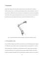
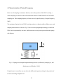
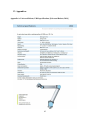
in an effort to allow people and industrial robots to work in close proximity. One such robot, of
particular interest to the sponsor of this project, is the Universal Robots UR10 (Fig. 1).
Fig. 1. The Universal Robots UR10 collaborative robot [Universal Robots, 2014].
2.1 Universal Robots, UR10
Universal Robots emphasizes the UR10’s smooth motion, precision handling and safety features.
The UR10 has 6 joints with 360 degrees of rotational freedom, a working radius of 1.3 meters,
and can support up to 10 kilograms. Universal Robots provides a unique Polyscope software
interface that allows the user to quickly and easily program multiple end points of the UR10
simply by manually moving the UR10 to a position and recording the position in its own global
14
coordinate system. The UR10 can then be easily programmed to move from point to point in
succession, with a positional repeatability of 0.1 mm according to Universal Robots. For a
complete list of the UR10’s specifications, see Appendix A.
The repeatability as reported by the manufacturer must be calculated according to
industrial standards. The International Standard Organization’s (ISO) 9283 is of particular
interest in that the standard specifies strict testing, environmental, and statistical standards to
follow in the analysis of an industrial robot. The user of an industrial robot can determine
repeatability characteristics and discover which variables affect the robot’s dynamic
characteristics by following ISO 9283 specifications.
2.2 International Standard 9283
ISO 9283 specifies guidelines for testing industrial robots [ISO 9283, 1998]. In order to be ISO
9283 compliant all tests must use the same paths, cycles, and environmental conditions. The
robot must be set up according to the manufacturer’s specifications with all necessary leveling
operations, alignment procedures, and functional testing completed. The testing must be
preceded by any appropriate warming up time, as dictated by the manufacturer.
Operational and environmental conditions must be normalized and repeated for each test.
Normal operating conditions include requirements for electric, hydraulic and pneumatic power,
power fluctuations and disturbances, and maximum safe operating limits. Environmental
conditions include temperature, relative humidity, electromagnetic and electrostatic fields, radio
frequency interference, atmospheric contaminants, and altitude limits.
All metrology equipment must be fully calibrated and the testing must account for any
and all uncertainty with respect to the metrology equipment, systematic errors, and calculation
15
errors. The measurements taken in the testing must be with reference to the tool center point
(TCP) inside the robot’s workspace [ISO 9283, 1998].
Robot characterization may take place after all of the preceding requirements have been
met.
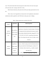
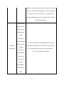
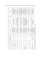
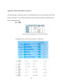
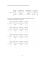
Table 1 shows a list of applicable test characteristics, brief explanations, and statistical
methods that could be applicable to the UR10 based on the project team’s findings.
Table 1. Robot characteristics as defined in ISO 9283.
characteristics
explanation
method/equations
to test
define the limit band (repeatability value or as specified by
manufacturer); elapsed time from the instance of the initial
how quickly a
position
crossing into the limit band until the instance when the
robot can stop
robot remains within the limit band; using path "P1 P5
stabilization
at the attained
P4 P3 P2 P1"; repeat this procedure three
time
pose
times, for each pose the mean value of t of three cycles is
calculated
robot
maximum distance from the attained position after the
capability to
instance of initial crossing into the limit band and when the
position
make smooth
robot goes outside the limit band again; overshoot, OV, = 0
overshoot
and accurate
if maximum value measured,
limit band; max
stops at
attained poses
, is smaller or equal to
√
16
; test
conditions: 100% rated load: 100%, 50% and 10% of rated
velocity; 10% rated load (optional): 100%, 50% and 10%
of rated velocity; all for one pose, 3 cycles same as
position stabilization time; use maximum value of three
times of measurement
time between
departure from
and arrival at a
stationary state
when
traversing a
predetermined
use 100% rated velocity and in addition test shall be
distance and/or
minimum
performed with optimized velocities for each part of the
sweeping
posing time
cycle if applicable to achieve a shorter posing time.; 3
through a
cycles; 100% and 10% rated load.
predetermined
angle under
pose-to-pose
control;
including pose
stabilization
time
17
unit: mm/N with reference to the base coordinate. Forces
used in the tests shall be applied in three directions, both
maximum
positive and negative, parallel to the axes of the base
amount of
coordinate system. Forces increase in steps of 10% of rated
displacement
load up to 10% of rated load, one direction at a time;
per unit of
measure the corresponding displacement of each force and
applied load.
direction; with servos on and brakes off. repeat three times
static
compliance
for each direction; with center of mechanical interface
placed at P1 (defined in pose section)
closeness of
agreement
for position:
between the
to n);
attained poses
pose
̅
; ̅
∑
̅
√
(with j from 1
̅
and ̅ ̅ ̅ as in pose accuracy.
̅
√
∑
̅
;
. For
after n repeat
repeatability
visits to the
orientation:
∑
√
̅
. (same for angle b and c)
(position only)
same
Cycles: path 1 P1, path 2 P1, path 3 P1; path 1
command pose
P2, path 2 P2, path 3 P2; path 1 P4, path 2 P4,
in the same
path 3 P4; repeat 30 cycles
direction
variation of
for position. Same for
drift of pose
pose
repeatability
orientation. Other requirements same as drift of pose
repeatability
(position only)
accuracy
over a
18
specified time,
T
Of the methods found in
Table 1, the sponsor indicated interest in pose repeatability in reference to position only,
which corresponded to the ability of the UR10 to return to a set of coordinates in three
dimensional space. Note that as such, of the six potential degrees of freedom of the UR10, the
repeatability analysis accounts for the coordinate tool position and not the angular position that
would determine the UR10’s tool face orientation.
2.2.2 ISO Technical Report 13309:1995
As an addendum to ISO 9283, the International Standards Organization published a technical
report outlining methods by which one could analyze industrial robots according to the
guidelines written in ISO 9283. The report describes eight types of performance measuring
methods and includes potential limitations of each method [ISO13309, 1995]. The two types of
methods deemed most useful to the sponsor’s interests were:
Trilateration Methods – the measurement of distances from a single point, P at the
robot’s tool tip, to two observation locations allows the calculation of point P, Fig. 2
Inertial Measuring Methods – the attachment of accelerometers and gyroscopes to the
tool tip allows characterization of the robot’s pose and path provided the initial position
is known, Fig. 3
These methods were extrapolated to fit the UR10 and evaluated alongside methods developed by
the project team.
19
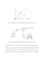
Fig. 2. Calculation of point P using trilateration in 2D [Thomas and Ros, 2005].
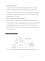
Fig. 3. Inertial measurement unit attached to a robotic arm [ISO 13309, 1995].
Please note that Fig. 2 shows a two dimensional representation of the Trilateration method, in
which the (x, y) coordinate position of P can be found using the distances ̅̅̅̅̅ and ̅̅̅̅̅ as radii
of circles, where the point P lies on the intersection of the two circles [3]. The method used in
calculating a robot’s tool tip position requires three dimensions, and thus the simultaneous
20
solution of three quadratic equations. This topic is further developed in the section titled “3.1
Trilateration Methods”.
21
3. Generation and Comparison of Test Methods
Based on the sponsor’s interests and ISO 9283, the methods chosen for evaluation had to meet
the following constraints:
Minimum resolution of 0.01 mm
Total cost no greater than $5000
Capability to apply 10%, 50%, and 100% of maximum payload (1, 5, and 10 kg
respectively)
Measurement of 3 Degrees of Freedom (X, Y, Z)
Measure five positions, thirty times each
Five methods were chosen for evaluation using the above constraints. These five methods
were composed of two trilateration methods, an Inertial Measuring Unit (IMU), a laser and
optics based tracking system, Micro Electromechanical Sensor (MEMS) mirrors, and a contact
method using a displacement sensor. The following sections briefly describe each method
including potential positive and negative factors associated with each method. For full
explanations of the considered test methods, including implementation and data processing, see
Appendix B.
3.1 Trilateration Methods
Trilateration techniques involve the use of algebra in conjunction with three length
measurements to a point of interest, P, to find the Cartesian coordinates of point P (Fig. 2). The
ISO technical report provided two suggested methods for trilateration location of a robot tool tip:
cable trilateration and sonic trilateration [ISO 13309, 1995].
22
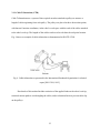
3.1.1 Cable Trilateration (CTM)
Cable Trilateration uses a system of three optical encoders attached to pulleys to measure a
length of cable originating from each pulley. The pulleys are placed at three observation points,
with known Cartesian coordinates, in the robot’s work space with the ends of the cables attached
to the robot’s tool tip. The lengths of the cables can be used to calculate the tool point location.
Fig. 4 shows an example of cable trilateration as demonstrated in ISO/TR 13309.
Fig. 4. Cable trilateration as presented in the International Standards Organization’s technical
report [ISO 13309, 1995].
Drawbacks of this method include restriction of the applied loads on the robot’s tool tip,
restricted motion paths to avoid tangling the cables, and acceleration limits to prevent cable slip
on the pulleys.
23
3.1.2 Ultrasonic Trilateration (UTM)
Ultrasonic trilateration uses three ultrasonic microphones placed at known observation points in
combination with an ultrasonic sound generator attached to the robot’s tool tip [ISO 13309,
1995]. The microphones measure pulses from the generator and the time between receiving each
pulse can be used to calculate the length from the microphone to the generator. The three lengths
allow tool tip calculation using the trilateration method. Fig. 5 shows an example of Ultrasonic
Trilateration. Drawbacks include fluctuations in ultrasonic intensity due to absorption effects at
high levels of humidity and potential interference to other equipment exposed to ultrasonic
pulses.
Fig. 5. Ultrasonic trilateration as presented in the International Standards Organization's
technical report [ISO 13309, 1995].
24
3.2 Inertial Measuring Unit (IMU)
The inertial measurement unit (Fig. 3) is a package of three accelerometers and three gyroscopes
that can be attached to the robot’s tool tip [ISO 13309, 1995]. When the initial position of the
UR10 is known, the accelerations and angles read by the sensors can be used in combination
with differential equations to calculate the final position of the UR10.
The IMU method suffers from compounding error in that the known acceleration must be
integrated twice to find position – any errors in the acceleration will be magnified in the final
position. Furthermore, as the robot’s tool tip continues to move, the superposition of error in the
acceleration causes extreme compounding of inaccuracies unless calibration is performed at each
position.
3.3 Laser Tracking Camera System (LTCS)
The LTCS is a new method designed by the project team to operate using the detectability of the
center of a beam of light based on the Gaussian distribution of light intensity from a laser beam.
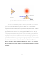
Fig. 6 illustrates how the center of a laser beam could be found using light intensity distribution
across camera pixels based on the Gaussian distribution. The highest intensity of light is found at
the center of the beam, with a normal (Gaussian) distribution of the intensity along the X and Y
axes. The respective maximum intensities on the X and Y axes yield a coordinate location of the
beam center on the XY plane. Cameras would be used as photo-detectors to find the center of
laser beams in the LTCS method.
25
Fig. 6. Use of Gaussian distribution to find the center of a laser beam.
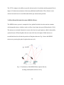
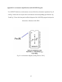
Three cameras positioned orthogonally to each other point towards a single location in
space, which would be the UR10’s final position. The UR10 carries an “Optical Head,”
composed of a laser and two beam splitters to generate three orthogonal laser beams. The beams
are calibrated to point to the center of the camera positioned along the laser’s axis when the
UR10 is at its position of interest, after which the UR10 moves to another position and back to
its calibrated position. Based on any displacement in the three centers of the laser beams at the
calibrated position, the system is able to measure and report the repeatability of the robot in three
dimensions. Camera systems, or “Detector Sub-systems,” can be placed at any position of
interest to determine the UR10’s repeatability at that point. Fig. 7 and Fig. 8 show a close up of
the UR10 outfitted with the system and the LTCS in place to measure repeatability at two points,
respectively.
26
Fig. 7. Close up view of the optical head and detector sub-system attached to the UR10.
Fig. 8. The UR10 outfitted with the optical head and two detector systems to evaluate
repeatability at two points.
27
The LTCS is unique in its ability to provide sub-micron level resolution and the potential for six
degree of freedom measurements without any additional modifications. These features come
with an increased cost of several thousand dollars per measurement position.
3.4 MicroElectroMechanical Systems (MEMS) Mirrors
The MEMS mirrors system is comprised of two gimbal-less dual-axis micro-mirror scanners
with integrated mirrors, which are used to reflect a laser beam into space [Mirrorcletech, 2014].
The mirrors are activated alternatively to move the laser in a spiral pattern, which is detected by
a photo-detector. When the photo-detector senses the laser, the angles of both mirrors are
recorded and used to calculate the position of the photo detector. Fig. 9 shows the MEMS
mirrors set up tracing the path of a photo detector at (b).
Fig. 9. Visualization of the MEMS Mirrors photo detector,
tracking method [Mirrorcletech, 2014].
28
3.5 Direct Contact Method (DCM)
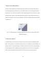
The direct contact method uses a displacement sensor attached to the tool tip of the UR10 to
record the displacement of the sensor tip as the UR10 touches several measurement positions
along an axis. Fig. 10 shows an example of using a stepped gauge block to provide five contact
positions along a single axis. By performing statistical analyses on the displacements across a
sample of contacts for each axis, the repeatability of the UR10 could be determined for all three
coordinate axes.
Displacement
Sensor
Fig. 10. Conceptualization of a stepped gauge block to provide five contact points for the
displacement sensor.
3.6 Selection of a Method
A decision matrix was developed as a comparison metric between the six methods described
above. These systems were evaluated according to their cost, resolution, accuracy, mobility, setup time, number of measureable degrees of freedom, and necessity for software programming.
For an explanation of the weighting system and equations used in the matrix, see Appendix C.
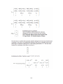
Table 2 shows the method evaluation with the DCM proving to be the optimal system.
29
Table 2. Decision matrix used for method selection.
3.7 Implementation of the Direct Contact Method
The DCM characterizes a robot’s repeatability by recording the robot’s ability to return to a point
on a uniaxial displacement sensor’s measuring range. In practice, the method involves teaching
the robot five positions on each of the X, Y, and Z axes. Each position corresponds to a face on a
gauge block such that the displacement sensor will contact the block and read a displacement for
the axis perpendicular to the gauge block face. A more repeatable robot will achieve the same
displacement more often than a less repeatable one – the repeatability is calculated according to
the equations established in ISO 9283.
The full development of the DCM involves the selection of an appropriate sensor;
calibration of the sensor; implementation and attachment of the sensor fixture; design of an
appropriate gauge block; fabrication of necessary fixture and purchase of the gauge block;
verification of fabricated materials; development of a data collection procedure and
accompanying software; data collection; and presentation of the data results.
30
In an effort to choose an appropriate sensor, the project team performed a dynamic
analysis of the UR10 to find the natural frequency of oscillation for the tool tip. The result of this
analysis was a minimum sampling rate, which led to the selection of the displacement sensor.
31
4. Characterization of Natural Frequency
In the case of sampling a continuous function, such as the position of the UR10’s tool tip, a
certain sampling rate must be achieved such that the function is band limited to one half of the
sampling rate. This sampling frequency is known as the Nyquist frequency [Nyquist Frequency,
2002].
The continuous function for the UR10’s tool tip position is a function of the stiffness, mass, and
damping characteristics of the arm. Fig. 11 shows a mass-spring-dashpot analogy in which the
UR10 can be represented by the mass, while the motors at each joint represent both the springs
and dashpots.
Fig. 11. Spring, mass, dashpot diagram showing mass (m), stiffness (k), damping (c), and
displacement (x) [Khanlou, 2014].
Using Newton’s second law one can derive the differential equation solving for the position of
the mass according to Equation 4.1.
32
̈
̇
(4.1)
Where x is the position of the mass, c is the damping ratio, m is the mass, and k is the stiffness.
Fig. 12 shows a plot of the underdamped UR10 motion, which is the result of the robot
oscillating as it approaches a position based on its attempts to correct itself. The underdamped
motion is compared to both over damped and critically damped systems.
Fig. 12. Plots of over, critically, and under damped systems [The Student Room, 2014].
The rate at which the robot oscillates in its correction is the natural frequency of
vibration. Any sensor used to measure the positional characteristics of the UR10 must have a
sampling rate at least equal to two times the natural frequency of oscillation of the UR10
according to the Nyquist Criterion [Nyquist Frequency, 2002]. With the use of MEMS
33
accelerometers, an analysis of the vibrational characteristics of the UR10 allowed the selection of
an appropriate sensor.
4.1 MEMS Accelerometers
MEMS accelerometers use internal cantilever beams with masses and magnets attached to
measure the acceleration experienced by the accelerometer according to changing capacitance
[Analog Devices, 2014]. In the case of the UR10, the attachment of accelerometers to the tool tip
allowed for measurement and recording of changing accelerations as the UR10 moved from
position to position. These accelerations correspond to the dynamic characteristics of the UR10,
namely, the natural frequencies of vibration of the robot.
Two dual-axis 35g MEMS accelerometers were attached to the UR10 tool tip using a
fixture fabricated using a Dimensional Rapid Prototype Machine such that the UR10’s tool tip
mass was minimally affected by the fixture. Each accelerometer was capable of measuring up to
35g’s (343 m/s2) of acceleration at 55 mV/g and can be seen mounted to the accelerometer
fixture along with their respective measuring axis in
Fig. 13.
Once the accelerometers were attached to the UR10 a LABVIEW program was run in
conjunction with the UR10’s motion to acquire vibration data. For more information regarding
the specifications of the accelerometers and the LABVIEW program see Appendix D.
34
Fig. 13. The accelerometer experiment set up showing the two accelerometers, coordinate
system, and ABS fixture.
4.2 Vibrations
The purpose of the vibrations testing was to determine the natural frequency of vibration for the
UR10 in regards to the three principal axes: X, Y, and Z. The experiment aimed to collect data
from the accelerometers using motion along each of the three axes of interest at different
accelerations.
The UR10 was taught two positions along a single axis – an initial position (position 1) at
which the robot started the data acquisition and a final position (position 2) where the robot
stopped its motion. The UR10 was programmed to send a DC voltage to trigger acquisition at
position 1, after which the robot moved to position 2 along the axis. After reaching position 2 the
UR10 stopped and the LABVIEW program continued to collect data for 5 seconds. Fig. 14, Fig.
15, and Fig. 16 show representations of the UR10’s displacement, velocity, and acceleration for
the vibration experiment. All three of these figures correspond to measurements along the XAxis.
35
The procedure was run along each of the three principal axes (X, Y, and Z), for five trials
each at accelerations of 0.2g, 0.4g, 0.6g, 0.8g, and 1g.
36
Fig. 14. The UR10's tool tip displacement along the X axis for the vibration experiment.
Fig. 15. The UR10's tool tip velocity along the X axis for the vibration experiment.
37
Fig. 16. The UR10's tool tip acceleration along the X axis for the vibration experiment.
The UR10 was also subject to several Impact Tests in which the UR10 was positioned
and left stationary to simulate a cantilever beam based on the fixed base and free tool tip – in this
way, the UR10 was most similar to the mass-spring-dashpot analogy described above. The robot
was then lightly struck with a white rubber mallet, a dark mallet, a hand on the second to last
link, and hand on the tool tip. The table that the UR10 was mounted to was also struck with a
hammer.
4.3 Experimental Results
The data collected during the vibrations experiments were first plotted in the time domain in an
effort to confirm the expected acceleration trends of acceleration from zero to constant velocity;
maintenance of constant velocity; and deceleration from constant to zero velocity as exhibited in
Fig. 16. A representative graph can be seen in Fig. 17– all motion plots followed the pattern seen
38
in this graph. Following the confirmation of the expected accelerations pattern, a Fast Fourier
Transform (FFT) was used to convert the data into the frequency domain (Fig. 18).
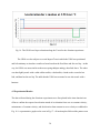
Vibration at Time Domain
Acceleration of UR10: 9.81 m/s2 in X-Direction
0.2
Magnitude [V]
0.15
0.1
0.05
0
-0.05
-0.1
0.000.250.500.751.001.251.491.741.992.242.492.742.993.243.493.743.984.234.484.734.98
Time [s]
Fig. 17. Time domain plot of the UR10's vibrations for X Axis motion.
39
Fig. 18. Fast Fourier Transform of accelerometer data for X motion with noise.
After de-convolving the noise out of the data, two peaks emerged in the frequency data
for the motion tests at roughly 30 and 125 Hz as represented by Fig. 19. These peaks were seen
in the vibrations along all three test axes (X, Y, and Z). The Impact Tests produced a peak at 125
Hz as well.
Table 3 shows the results of the vibrational analyses in which the frequency peaks along
each axis were averaged to find the natural frequency of that axis.
40
Fig. 19. Deconvolved vibration data showing frequency peaks at 30 and 125 Hz.
Table 3. Representative results of the vibration experiment, shown for the Z axis.
41
4.3.1 Interpretation
The data from the accelerometer experiment resulted in three findings:
Amplitude of vibration increases with increased tool tip acceleration
Frequency of vibration is not related to acceleration
The natural frequency of the robot is 125 Hz
Fig. 20,Fig. 21, and Fig. 22 show plots of the amplitude of the vibration at 125 Hz versus
tool tip acceleration. The amplitude of the vibration increases with the acceleration along all
three axes, as expected based on the increase in forces required to create larger accelerations at
the tool tip.
Fig. 23,
Fig. 24, and Fig. 25 show the relationship between the natural frequency of vibration and
increased tool tip acceleration. As expected of the natural frequency, the UR10 oscillates at the
same rate independently from the acceleration. The presence of this relationship further
reinforces the next claim – that the natural frequency of the robot is 125 Hz.
42
Fig. 20. Amplitude of vibration versus acceleration along the X axis.
Fig. 21. Amplitude of vibration versus acceleration along the Y axis.
43
Fig. 22. Amplitude of vibration versus acceleration along the Z-axis.
Fig. 23. Frequency of vibration versus acceleration along the X axis.
44
Fig. 24. Frequency of vibration versus acceleration along the Y axis.
Fig. 25. Frequency of vibration versus acceleration along the Z axis.
Based on the presence of a 125 Hz frequency in both the dynamic and impact vibration
tests, the team concluded that the natural frequency of the UR10 was 125 Hz. Such a claim is
45
validated through the concept of the natural frequency, which is an inherent characteristic of a
system that will always appear when the system is stimulated, regardless of the stimulus type.
Using the natural frequency of 125 Hz and the concept of the Nyquist frequency, the
team determined that any sensor used to measure the position of the UR10 must have a sampling
frequency of at least 250 Hz.
46
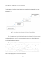
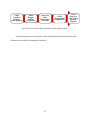
5. Realization of the Direct Contact Method
The development of the Direct Contact Method was accomplished according to the flow chart
shown in Fig. 26.
Fig. 26. Steps taken in the realization of the Direct Contact Method.
The selection of sensor involved the identification and evaluation of displacement sensors
according to the project’s needs. The two most appropriate sensors were ordered and tested to
see which performed better in practice.
The synthesis of hardware involved the design of a fixture to mount the selected sensor to
the UR10. The fixture was optimized, then fabricated. A gauge block was also designed and
fabricated to provide the contact positions for the repeatability procedure.
For the DCM to function properly, a LABVIEW program was needed to collect data
from the displacement sensor. This LABVIEW program was written to communicate with the
UR10’s Polyscope program for accurate data acquisition.
47
A MATLAB script was written to process and output the results of the repeatability
procedure according to the equations given in ISO 9283.
48
6. Selection of Sensor
The Direct Contact Method, required a sensor with a sampling rate of at least 250 Hz. The
selection of a suitable sensor involved the research and comparison of linear potentiometers.
Four distinct models were selected and compared based on: cost, resolution, repeatability,
measurement range, signal conditioning, signal output, signal to noise ratio, shipping time, and
mounting type. For an explanation of the aforementioned criteria and equations used to evaluate
the sensors, see Appendix E.
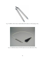
The most suitable sensors were the Omega GP911 Linear Variable Differential
Transducer (LVDT, Fig. 27), LORD MicroStrain Sub-miniature DVRT (Fig. 28) Honeywell
LVDT, and Mitutoyo electronic displacement indicator.
Table 4 shows the evaluation of the sensors. Based on the results of the decision matrix,
the Omega GP911 and MicroStrain SG-DVRT were ordered for testing purposes. Note that the
Mitutoyo indicator was ruled out because the sensor was only able to measure a maximum and
minimum deflection, which would not work with the goals of the DCM.
After arrival, the Omega and MicroStrain displacement transducers were set up in
Worcester Polytechnic Institute’s (WPI) Center for Holographic Studies and Laser micromechaTronics according to the manufacturer’s instructions. Both sensors were then calibrated
and evaluated using a linear actuator and micro-stage to validate the manufacturer’s claims for
repeatability and linearity.
49
Fig. 27. OMEGA GP911 Linear Variable Differential Transducer (LVDT) [Omega, 2014].
Fig. 28. LORD MicroStrain SG-DVRT displacement sensor [Microstrain, 2014].
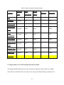
50
Table 4. Sensor evaluation decision matrix.
Category
Lord
LVDT
Category
Mitutoyo
Honeywell
Value
MicroStrain
Omega
Cost
10 points
84%
94%
-
86%
Resolution
5 points
95%
95%
-
99%
Repeatability
10 points
99%
87%
-
80%
10 points
100%
100%
-
100%
15 points
85%
100%
-
85%
10 points
100%
100%
-
100%
15 points
98%
90%
-
Not Provided
Shipping Time
20 points
80%
100%
-
20%
Mount Type
5 points
100%
75%
-
100%
Total Score
100 points
91%
95%
-
63.26%
Measurement
Range
Signal
Conditioning
Signal Output
Signal to Noise
Ratio
6.1 Omega GP911-2.5-S LVDT and MicroStrain SG-DVRT
The Omega and MicroStrain sensors were evaluated to determine which of the two would be
most effective in the DCM. The two sensors were set-up and calibrated using a Newport LTA-
51
HS actuator and micro-stage, which had 0.5 micron repeatability, in order to determine which
sensor performed better in practice.
6.1.1 Calibration
Fig. 29 andFig. 30 show the Omega displacement transducer mounted to the actuator stage. The
MicroStrain DVRT was mounted and tested in the same way.
Fig. 29. Top view of the OMEGA LVDT mounted to a Newport actuator
and micro-stage for calibration.
A LabVIEW program was used to control the stage, which moved in 0.5 mm increments
across the measuring range of each sensor. Ten iterations were performed at each position and
the resulting data was processed in MATLAB. A Student’s t-test was used to determine that a
linear fit of displacement to each sensor’s voltage would give sufficient accuracy (Appendix F).
52
The calibration resulted in calculated repeatability, accuracy, and linearity for each of the two
sensors. Table 5 shows the results of the calibration procedures - the Omega LVDT
outperformed the MicroStrain SG-DVRT.
Fig. 30. Side view of the OMEGA LVDT mounted to the Newport actuator
and micro-stage for calibration.
Note that the MicroStrain sensor proved to be extremely susceptible to magnetic fields,
which caused the sensor to perform poorly. In addition to being outperformed by the Omega
LVDT, the MicroStrain DVRT would not be an acceptable sensor without the addition of
magnetic shielding.
53
Table 5. Calibration results and analysis of the OMEGA LVDT and MicroStrain SG-DVRT.
54
7. Synthesis of Hardware
The DCM required the ability to mount the Omega LVDT to the UR10 while meeting the
following basic requirements
Modular payload of 10%, 50%, and 100% of UR10’s capability
Minimum length to keep loading closest to true center of UR10 tool tip
Non-interfering natural frequency of vibration
Integrated wire port for plug and play capability
Furthermore, the DCM required a gauge block to provide five contact points for each axis –
see section “7.2 Gauge Block Design.” Mechanical drawings for all of the hardware components
can be found in Appendix G.
7.1 Design of Fixture
A fixture was designed to house the LVDT and wiring internally, with the outside of the fixture
serving as an attachment point for increased payloads. Fig. 31 shows the preliminary design in an
exploded view featuring: a flange with matching pilot and bolt circle to the UR10; a hollow shaft
to house the LVDT body and wiring internally; and the outside diameter of the shaft serving as a
mount for increased payloads in the form of oversized washers.
55
Flange
Sensor
Payload
Lock Nut
Fig. 31. Sensor fixture design shown with representative sensor, payload, and locking nut.
7.1.1 Attachment of LVDT
As shown in Fig. 31, the LVDT can slip through the front of the fixture through a hole bored into
the shaft. The wire runs through the center of the shaft and out through a hole drilled through the
mounting flange. Once in place, the LVDT wire must be soldered to a five pin plug (Fig. 32) and
the LVDT body is held in place using a nylon tipped M5x0.8 set screw torqued to 0.8 Newtonmeters as specified by the GP911 User Manual.
56
Fig. 32. Back view of sensor fixture showing
the five-pin plug on the flat face of the flange.
7.1.2 Modulation of Payload
The washers were made from cast iron due to its high density, allowing for minimal washer
dimensions for the required payloads of 50% and 100% of the maximum payload. The washers
slide over the outside of the fixture’s shaft and are designed to maintain a center of gravity along
the UR10 tool tip’s central axis. The first 1.5” of the outer shaft is threaded with 1.25”X 7 UNC
threads such that the washer can be locked in place using two 1.25” jam nuts. The washers have
four clearance holes to allow the heads of the M6 bolts (used to mount the fixture to the UR10)
to sit within the washers – aiding in alignment and prevention of vibrations in the washers.
7.1.3 Analysis
The fixture was optimized using Finite Element Analysis (FEA), run through the ANSYS client
within SolidWorks 2013. The goal of this optimization was to:
Minimize cantilever length of the shaft
Maintain fixture mass of 1 kg
57
Minimize washer dimensions
Minimize cost of materials
Natural frequency at least ten times that of the UR10 with max payload
7.1.1.1 Assumptions and Results
The fixture material chosen for the analysis was Series 304 Stainless Steel, which was chosen to
minimize any potential magnetic interference. The fixture was fixed about the back of the flange
where it connects to the UR10 and a force of 1000 N was applied to the shaft to simulate the
worst case loading on the fixture. The results, shown in Fig. 33, demonstrate the maximum Von
Mises stress on the shaft after optimization.
Fig. 33. Von Mises stresses in the sensor fixture.
At the base of the cantilever, the stress is 2.3 MPa giving a minimum safety factor of 89.
This safety factor shows that the dimensional needs relating to securing the LVDT and
58
decreasing the outer diameter of the payload were more critical to the design than the stresses
caused by the applied loads.
The natural frequency of vibration with the 10kg payload is 1687 Hz as seen in Fig. 34.
This frequency is the lowest frequency of the fixture as evidenced by Equation (6.1).
√
(6.1)
Fig. 34. Vibrational analysis of the sensor fixture showing a max frequency of 1687 Hz.
7.2 Gauge Block Design
The gauge block was designed to provide five measurement positions for the UR10 based on
ISO 9283 guidelines. Based on the ability for the LVDT to measure repeatability for a single axis
at a time, the gauge was designed with three faces each having five positions to allow
appropriate measurements for all three principal axes. The gauge block was designed to take into
59
account both the surface roughness of the gauge as well as thermo mechanical expansions to
ensure dimensional accuracy during testing.
A checkered pattern of pockets was designed to accomplish the above while
simultaneously keeping the volume minimal for sensor clearance and preventing the largest
washer from contacting the test table. Fig. 35, shows the realization of this goal.
The checkered pockets were designed to be large enough to account for the diameter of
the sensor and any possible error in an effort to reduce chances of a damaging collision. The
overall size of the block was chosen such that the range of payloads would not collide with the
mounting table and in order to prevent a collision between the fixture and the block.
Fig. 35. Gauge block assembled and mounted to an optical breadboard.
60
Aluminum 7075 was selected as the manufacturing material in an effort to minimize
micron level errors caused by temperature fluctuations. Low head M5 bolts were chosen to
mount the gauge block to the plate, while ¼-20 UNC bolts were necessary to mount the plate to
the sponsor’s optical breadboard table. Four slots for the ¼-20 bolts allowed alignment of the
gauge such that the UR10 tool face and front gauge face were parallel.
7.3 Fabrication
The manufacturing of the fixture components was completed using the machine shop in
Washburn/Higgins Labs in addition to a lathe at Reich USA (Mahwah, NJ) capable of turning
cast iron with a diameter of 6”.
The washers were fabricated using 6” Diameter cylindrical bar stock ordered from
McMaster Carr. The stock was cut to the rough size of the washers using a band saw, then faced
to 2.75” in length on a manual lathe. The 50% payload washer was turned down to 4” outer
diameter, then both washers were bored to the fixture shaft’s diameter with a sliding tolerance.
The M6 bolt head counter bores were done with a Haas MiniMill.
The fixture was made using 3.5” diameter Series 304 Stainless Steel. The front shaft and
sensor holding profile were turned down on a Haas T1 lathe, then bored to fit the LVDT. The
back pilot was turned on the same lathe and bored to allow the LVDT wires to run through. A
Haas MiniMill was used to create the flange profile and M6 bolt circle, while a drill press was
used for the set screw and plug holes. Fig. 36 shows the finished fixture mounted to the UR10
with the largest payload attached.
61
Fig. 36. Fixture with 10 kg payload mounted to the UR10.
The team chose to manufacture the gauge block in Washburn Shop rather than purchase a
certified block from a third-party based on the need for a customized block with five
measurement positions on three faces. The customized gauge blocks that were researched
required a minimum 6-week lead time for manufacturing at a third-party machine shop and an
addition of several weeks for certification. Although dimensional tolerances for the gauge block
were important, the DCM procedure does not actually measure position, but displacement, and as
such tolerances beyond the 0.02 mm achievable in WPI’s Washburn Shop were not necessary –
leading to the selection of a Haas MiniMill for the pocketing operation on the gauge block. Fig.
36 shows the completed assembly.
62
7.4 Validation of Fixture Assembly
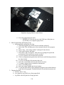
Every component was inspected and verified post-fabrication. The LVDT was pushed through
the front bore, soldered to the five pin plug and mounted within the fixture, then tested using the
sensor calibration procedure originally used for sensor evaluation.
63
8. Testing Procedure Overview
The testing procedure was developed to follow the flow chart shown in Fig. 37. The full Direct
Contact Method instruction manual can be found in Appendix L.
Fig. 37. Flow chart for the Direct Contact Method testing procedure.
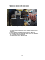
The hardware set-up involves mounting the sensor fixture to the UR10; mounting the
gauge block to the table; connecting wires from the UR10 to the LDX signal conditioner;
connecting the sensor to the LDX; and connecting the signal conditioner to the Data Acquisition
(DAQ) box, which transfers data to a computer. Fig. 38 shows the laboratory set-up. The UR10
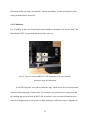
provides power to the signal conditioner, which powers the LVDT and filters out the sensor’s
noise before passing the signal to the DAQ box and laptop.
64
Fig. 38. Laboratory set-up for the Direct Contact Method.
After hardware set-up, the UR10 must be taught all of the necessary contact positions
along the gauge block. This step involves aligning the gauge block to the UR10 (Fig. 39) and
manually teaching the robot to touch five positions on each face. These positions correspond to
the five pockets on the vertical faces of the gauge and four pockets plus the raised middle surface
on the top face.
65
Fig. 39. Alignment procedure for the gauge block and UR10.
The data acquisition at each position follows the sequence shown in Fig. 40: the UR10
moves to touch a gauge face; the UR10 sends a signal to start data acquisition; the UR10 waits 2
seconds; the UR10 moves to the next position and the process repeats. A single full testing
procedure involves the robot touching each of the fifteen gauge block positions 30 times each.
Each test can be modified to allow repeatability testing with modified payload and acceleration:
payload can be changed by attaching/removing the oversized washers and acceleration can be
modified using the UR10 control pad. The project team ran tests with payloads of 1, 5, and 10 kg
and accelerations of 0.2, 0.5, and 1.0g.
66
UR10
Contacts
Position,
holds position
UR10
Triggers
Start of
Acquisition
Probe Tip
Data
Collected for
2 Seconds
UR10
Triggers End
of Acquisition
UR10
Moves to
Next Step of
Block &
Repeats
Fig. 40. Process flow for data acquisition at each gauge location.
Software programs were developed to collect and analyze the data as described in the
following section titled “Development of Software.”
67
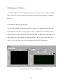
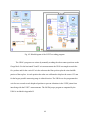
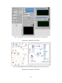
9. Development of Software
A LabVIEW program and UR10 Polyscope Program were developed for recording repeatability
data. A MATLAB script was written to process the data and output repeatability according to
ISO 9283.
9.1 LabVIEW and Polyscope Program
The LabVIEW program was written to receive two separate AC voltages from the UR10 and
LVDT. Whenever the UR10’s voltage signal was above 3V the program recorded the LVDT’s
voltage for two seconds and wrote the data to an excel sheet. The program was able to record as
many points as necessary until the user stopped LabVIEW, due to a nested while loop. Fig. 41
and Fig. 42 show the front panel and block diagram from the LabVIEW program.
Fig. 41. Front panel of the recording program.
68
Fig. 42. Block diagram of the LVDT recording program.
The UR10’s program was written by manually teaching the robot contact positions on the
Gauge block. For the horizontal X and Y axis measurements the UR10 was taught to touch the
five pockets and for the vertical Z axis the robot touched four pockets plus the raised middle
portion of the top face. At each position the robot was calibrated to displace the sensor 1.25 mm
for the largest possible measuring range in either direction. The UR10 was also programmed to
wait for two seconds at each displaced position to prevent vibrations in the LVDT piston from
interfering with the LVDT’s measurements. The full Polyscope program as outputted by the
UR10 is included in Appendix H.
69
9.2 MATLAB Analysis
The MATLAB script was written to process all of the voltage files recorded from LabVIEW.
The script prompts a user to input several parameters including the sampling rate, sampling
duration, iterations per position, positions tested per test, number of axes (directions) tested,
number of payloads tested, and number of payloads tested. Based on the user’s inputs the script
will output repeatability values for each test. The full MATLAB script is included in Appendix I.
70
10. Collection of Data
The UR10 was programmed to touch the five pockets on the two vertical faces of the gauge
block to characterize X and Y repeatability, in addition to four pockets and the middle surface of
the top plane of the block to characterize Z repeatability (Fig. 43).
Z
Y
X
Fig. 43. Gauge block with directional labels.
The UR10 sent a 5V DC signal to start the collection of data from the LVDT when the UR10
was at its final position for each measurement position. The UR10 then waited for 2 seconds,
sent out a 1V signal to turn off data collection, and moved to the next position along the same
face. The five measurement points on each axis were touched thirty times each before the UR10
71
moved to the next axis. In a single procedure the UR10 performed X, Y, and Z repeatability
measurements in that order. Each repeatability procedure took approximately 45 minutes over a
total of 9 tests.
10.1 Repeatability Parameters
The goal of the DCM was to characterize the repeatability of a collaborative robot as functions of
payload and acceleration. According to ISO 9283 the payload was tested at 10, 50, and 100% of
the UR10’s maximum capabilities, while the acceleration was 0.2, 0.5, and 1 g. The data
collection resulted in data files containing the LVDT’s displacement as it touched each of the
fifteen gauge block positions 30 times for the payloads and accelerations described above.
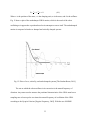
For the following analysis and explanation, increasing repeatability indicates that the
repeatability value became larger. For all cases, a smaller value for repeatability indicates higher
robot precision, which is more desirable.
10.1.1 Repeatability vs. Payload
ISO 9283 dictates that a robot should be evaluated at 10%, 50%, and 100% of its maximum
payload. To that end the repeatability procedure was run for all three payloads by attaching only
the fixture (1 kg); the 4” diameter washer and fixture (5 kg); and the 6” diameter washer and
fixture (10 kg); respectively.
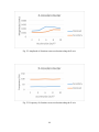
The analysis showed that the repeatability of the UR10 is independent of payload for the
X and Y directions. The average repeatability for X and Y is 0.05 and 0.04 mm respectively,
well within Universal Robots specification of 0.1mm.
72
For the Z direction repeatability deteriorates as payload increases. The UR10’s
repeatability increases from within manufacturer’s tolerances (0.06 mm at 1 kg) to outside the
tolerance (0.236 mm at 10 kg). The loss of repeatability is far less between 1 and 5 kg, than
between 5 and 10 kg – a change of 0.006 and 0.169 mm respectively. These results indicate a
threshold payload between 5 and 10 kg, after which the UR10 rapidly loses repeatability. The
overall increase in repeatability for the Z Direction can be explained by the loading of the UR10
– the load acts in the Z direction, indicating that for larger loads the arm will have to exert a
larger force in the Z direction, leading to larger amplitudes of oscillation and decreases in
repeatability. Additional statistical analysis is necessary to prove the accuracy of this claim, see
section “9.2 Statistical Analysis.”
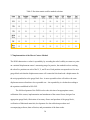
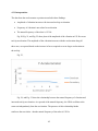
Table 6 shows the average repeatability for each direction at the three different payloads.
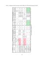
Note that for these tests the acceleration was a constant 0.2g; a data table containing all of the
individual data points collected during the 9 tests can be found in Appendix K. Fig. 44 shows a
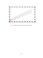
plot of Payload versus Repeatability as presented in Table 6.
73
Table 6. Average repeatability for the UR10 for
varying payloads with constant 0.2g acceleration.
Axis
X
Payload (kg) Avg. Repeatability (mm)
1
0.055
5
0.051
10
0.053
Y
1
5
10
0.041
0.029
0.044
Z
1
5
10
0.061
0.067
0.236
Fig. 44. Plot of Payload vs. Repeatability with acceleration constant at 0.2g.
74
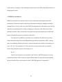
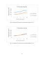
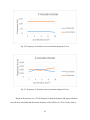
10.1.2 Repeatability versus Acceleration
The UR10 has a safety feature that automatically stops the arm from moving when any link in
the arm experiences a force of 150 Newtons. Based on this feature, the tool tip could reach a
maximum acceleration of 1.0g before the tool’s inertia caused a force in excess of 150 N (with
max payload). Therefore the repeatability of the UR10 was calculated as a function of 0.2, 0.5,
and 1.0g.
The data shows that repeatability deteriorates as acceleration increases for all directions.
With a payload of 1 kg, the X direction repeatability increased from 0.055 to 0.201 mm; the Y
direction repeatability increased from 0.041 to 0.063 mm; and the Z direction increased from
0.061 to 0.162 mm when the acceleration was increased from 0.2 to 1.0 g. These results show
that only Y direction repeatability remains within the UR10’s specifications at maximum
acceleration. The worst case repeatability was 0.285 mm for the Z Direction with maximum
payload and acceleration.
Fig. 45 shows a plot of the UR10’s repeatability as a function of acceleration for the X
direction, showing the trend of increasing repeatability with increasing acceleration.
75
Fig. 45. Repeatability as a function of acceleration in the X Direction.
10.2 Statistical Analysis
The UR10 performs as indicated by Universal Robots for payloads below 5 kg and accelerations
below 0.5g. These results indicate that for procedures in agreement with manufacturer’s
recommended speeds for the UR10, the UR10 will perform with a repeatability better than 0.1
mm.
A full statistical analysis is necessary to support the results found in the preliminary
analysis of the UR10. The number of necessary tests requires assumptions for the risk of
rejecting a true value and the risk of accepting a false null value during each test [Petruccelli et.
al., 1999]. To establish a 95% confidence level in the relationships established in section “8.1
Repeatability Parameters,” Eq. 10.1 should be used.
(10.1)
√
76
The number of samples, N, then depends on the mean of the samples, standard deviation of the
samples, and critical value from the normal distribution (z). For a 95% confidence interval, we
have Eq. 10.2 and 10.3, which respectively calculate the critical value from the normal
distribution and the number of samples required.
(10.2)
(10.3)
Based on the calculation of Eq. (10.2) and (10.3) using the mean and standard deviation from the
preliminary tests, each test should be run two more times, for a total of 24 more tests. Based on
the relationships described in “8.1 Repeatability Parameters,” two more tests would yield a 95%
confidence level of any single data point being within one standard deviation of the mean
repeatability values shown in Table 6.
77
11. Conclusions and Recommendations
The development of the Direct Contact Method was able to prove that collaborative robotic
repeatability can be measured using a uniaxial displacement sensor. The uses of MEMS
accelerometers allowed the selection of an appropriate sampling rate to accurately characterize
the position of the UR10 using the fixture and gauge block designed by the project team.
The accompanying LabVIEW and MATLAB software accurately collected and analyzed
data, leading to characterization of the UR10’s repeatability as functions of payload and
acceleration. Based on the results in “8.1 Repeatability Parameters,” the UR10 meets the
manufacturer’s tolerances for all cases with accelerations below 10 kg for the X and Y
directions, but does not meet manufacturer’s tolerances in the Z direction when the payload is
above 5 kg and/or when the acceleration is set above 0.5g.
The project team’s recommendations would be to use the UR10 for high precision
applications only when the UR10’s acceleration is below 0.5g to avoid the loss of repeatability in
the Z direction. Furthermore, the payload of such applications should remain below 5 kg if
possible.
The next step in the development of the Direct Contact Method is to refine the method
such that it can be used to evaluate other robots.
11.1 Future Work
The bulk of this project was focused on the development and verification of the Direct Contact
Method for evaluating the repeatability of collaborative robots. The results of the UR10’s
analysis prove the feasibility of the DCM, but the method requires further development before it
78
can be applied to other robots. Improvements to the DCM could be broken into refinements to
the hardware used in the method and the actual measurement process itself.
11.1.1 Refinement of Hardware
The fixture is designed specifically to mount to the UR10 as a single unit - a universal sensor
housing should be developed. Such a housing would be able to mount to an adapter plate that
contains the bolt housing bolt pattern/pilot on one side, and the required mounting configuration
of the robot to be tested on the other side. Other methods such as a housing that only needs to be
held by a robot’s gripper could also be investigated.
The gauge block could be improved if a suitable third party block with appropriate
surface finish and dimensional certification were found. Such a block would allow the testing of
multiple locations within the robot’s work space without the need to machine and measure
surface finish in house.
Alternatively to the improvements described above, two cantilever displacement
measuring systems could be added to the sensing fixture to reduce testing time. The LVDT
would remain along the robot tool’s Z axis, with the two cantilever sensors measuring
displacement along the X and Y axes, respectively. Such a system would allow the testing of all
three axes simultaneously, cutting testing time by 67%. If this development were implemented,
the gauge block would have to be redesigned to provide contact points for all three sensors
simultaneously. Furthermore, the Data Acquisition system would need two additional analog
input channels for processing the three voltages.
79
11.1.2. Refinement of Software
The method itself could be improved with a robot program that incorporates the geometry of the
gauge block such that the robot only needs to be taught the first position – the program would
include offsets for all other motions based on the preliminary coordinates. The measurement
method could also be combined with the robot in question’s characteristic Denavit-Hartenberg
parameters [Spong, 1989] as well as MEMS accelerometers to develop a full theoretical and
experimental dynamic model.
11.1.2.1 Analysis of Measurements vs. Denavit-Hartenberg (DH) Parameters
The DH parameters are a standardized method for evaluating the coordinate transformation from
the base to the tool tip of a multi-jointed (multiple degrees of freedom) robot. Such a method
allows the determination of the tool tip coordinates in the base (global) coordinate system using
the angles of each of the joints in the robotic arm. The DH parameters also allow the
characterization of dynamic properties by incorporating inertia, momentum, and forces/torques
applied to the robot [Spong, 1989].
The DH parameter calculations performed by the project team were not successful in
determining the forward kinematics of the UR10’s tool tip nor was the method successful in
calculating the inverse kinematics. The further development and troubleshooting of the DH
parameters would allow the combination of theoretical and measured repeatability to form a
more accurate model for the UR10. The DH parameters and matrix transformation for the
forward kinematics of the UR10 can be found in Appendix J.
80
11.1.2.2. Addition of Vibration Measurements
The addition of MEMS accelerometers to the LVDT fixture would allow the characterization of
vibrations that occurred during repeatability measurements. These vibrations could be used to
diagnose any potential changes in repeatability that occurred within a test or at certain positions
within a robot’s workspace.
11.2 Vision for the Direct Contact Method
This report described the development of the Direct Contact Method as a means for measuring
collaborative robotic arm repeatability. The design process involved the comparison of state of
the art methods for evaluating positional repeatability; selecting appropriate methods and
metrology equipment; calibrating and implementing the LVDT; designing, optimizing, and
fabricating the necessary fixture and gauge block; developing accompanying LabVIEW and
MATLAB programs; implementation and testing of the DCM using the UR10; and analyzing the
repeatability data to confirm the manufacturer’s specifications for the UR10.
The final deliverables to the sponsor were the full DCM method package- including
hardware, software, and a User Manual; a characterization of the UR10’s repeatability as
functions of payload and acceleration; and further recommendations for development of the
DCM such that other robots can be evaluated before purchase.
The use of the UR10 allowed a demonstration of the Direct Contact Method’s feasibility
for evaluating collaborative robot repeatability. It is the project team’s hope that the method
developed in this report will be of use to the sponsor and that further development of the DCM
will lead to increased implementation of low cost repeatability measuring solutions.
81
12. References
[1] Universal Robots. http://www.universal-robots.com, Last Accessed April 2014.
[2] ISO 9283. International Organization for Standardization, 1998.
[3] ISO 13309. International Organization for Standardization, 1995.
[4] Thomas, F. and Ros, L., “Revisiting Trilateration for Robot Localization,” IEEE Trans.
Robotics, 21(1): 93-101, 2005.
[5] Mirrorcle Technologies. http://www.mirrorcletech.com, Last Accessed April 2014.
[6] Nyquist Frequency. Cambridge Dictionary of Statistics, Cambridge University Press, UK
2002.
[7] Khanlou. http://www.khanlou.com, Last Accessed April 2014.
[8] The Student Room. http://www.thestudentroom.co.uk, Last Accessed April 2014.
[9] Analog Devices. http://www.analog.com, Last Accessed April 2014.
[10] Omega. GP911-2.5s LVDT, http://www.omega.com, Last Accessed April 2014.
[11] Microstrain. SG-DVRT-8mm, http://www.microstrain.com, Last Accessed April 2014.
[12] Petruccelli, J., Nandram, B., Chen, M., Applied Statistics for Engineers and Scientists,
Pearson, 1999.
[13] Spong, M.W., Robot Dynamics and Control, Ch. 3-4, John Wiley and Sons, 1989.
[14] Digikey. http://www.digikey.com, Last Accessed April 2014.
[15] IMU. http://www.wikimedia.org, Last Accessed April 2014.
82
13. Appendices
Appendix A: Universal Robots, UR10 specifications [Universal Robots, 2014]
83
Appendix B: Repeatability Methods Detailed Descriptions
MEMS Mirrors in 3D tracking application
How are we going to build it?
The MEMS mirrors system is comprised of two gimbal-less dual-axis micro-mirror scanners
with integrated mirrors, a NI USB DAQ-version 4-channel high voltage amplifier, a 5mW red
laser, a field programmable gate array (FPGA) board, 2 wide angle lenses, a photo-detector,
tracking software, and a laptop.
How are we going to integrate it into different positions?
The MEMS mirror tracking system tracks a photo-detector in a specified field of view, on one
plane. An end effector containing multiple (3-4) photo-detectors perpendicular to each other
could be incorporated to allow for tracking of the robot when it is facing different planes.
Additionally, the system is a mobile system and can be picked up and moved to different
positions with ease.
How are we going to calibrate it?
First the lasers must be modulated to continuously alternate. This calibration can be done
through programming software which accompanies the laser and the FPGA board.
The next step is to calibrate the photo-detector. The photo-detector is a 4-quadrant detector
which means it has 4 quadrants which provide additional information such as the position of the
laser on the detector. The detector and mirrors can then be programmed and calibrated using a
LabVIEW code to signal the system when the laser is centered on the target.
84
How are we going to use it?
The systems works by reflecting a laser off each micro-mirror through a wide angle lens into a
common volume. Through the use of tracking software, both mirrors search in a spiral pattern
from their origin (0 degree tilt) to maximum angles (up to 45 degrees when incorporating a wide
angle lens). When a 4 quadrant photo-detector comes into the field of view it relays a signal to
the FPGA board when it detects a laser. Since the photo-detector can only detect one laser at a
time the system is time-multiplexed by laser modulation. This means that the lasers are
continuously alternating.
Once the photo-detector has relayed a signal to the FPGA board, the system instantaneously
records the angle of the device’s x and y-axis in open-loop output values OX1 and OY1 through
the use of the high voltage amplifiers. Since the system is time-multiplexed, the second device
then provides an additional set of open loop angles OX2 and OY2. These angles are then used to
calculate a Z position.
How are we going to analyze the data it produces?
Using the output angles from the system and the following equations we can find the position of
the photo detector with
85
These equations can be integrated into the system to continuously calculate the position of the
end effector.
Cable Trilateration Method (CTM)
General Overview: The cable trilateration method uses the lengths of various cords attached to
the tool tip of a robot (End Effector) to determine the tool tips location in 3D space.
Fig. 46: ISO technical report [ISO 13309, 1995].
How are we going to build it?
The cable trilateration method typically uses a three or four pulley systems with optical encoders
attached to measure the length of cables originating from each pulley. To build the system we
would have to construct the pulleys with minimized cable slippage and minimized constant
tension on each cable as to not add undue load on the robot’s tool tip. Providing we could
86
achieve these characteristics, the pulleys are relatively simple in that they need only be free to
rotate around a vertical axis (in addition to the pulley’s own horizontal axis rotation) to track the
robot without becoming entangled. Furthermore, each pulley must have an optical encoder
attached to it by means of a shaft that rotates with the pulley such that the rotational position of
the pulley is always known. The length of the cord is equal to the radius of the pulley multiplied
by the number of revolutions of the pulley.
How are we going to integrate it into different positions?
The cable trilateration method can measure any number of points and is capable of recording
path of motion as well as assessing positional repeatability. To integrate the CTM to record
multiple positions we would simply have to teach/program the robot to go to multiple positions,
the cable system does not require any extra effort to measure additional points as it constantly
measures and plots the tool tip’s position in space.
How are we going to calibrate it?
The typical calibration method requires two steps:
1) Calibrating the encoders – the pulleys must be placed in an approximately equilateral
triangle in the robot’s workspace. The cord of each pulley must be pulled to the adjacent
pulley in order to measure and record the distance between each of the pulleys.
2) Robot Calibration – the cords must be attached to the robot’s tool tip, then the robot must
move through many (~50) points in its workspace while the CTM system measures
position. The system then compares the robot’s measured position to the CTM true
position to establish a filter to account for any kinematic inaccuracies of the robot
87
How are we going to use it?
We would use a CTM system to characterize the repeatability of the robot according to
ISO9283. The CTM method is capable of performing all of the tests in ISO9283, but we
would only need to perform the pose repeatability tests. Typically, these involve measuring
the repeatability at 5 unique positions approached from 3-directions, which could easily be
accomplished using a CTM system.
How are we going to analyze the data it produces?
Commercial software is capable of directly outputting the results of tests such as those
described in ISO9283. Furthermore, typical software shows a plot of the robot’s position and
3-D coordinates in the form of (x,y,z) in real time. To that end, whether we design or
purchase software for a CTM system, we would be able to output position and repeatability
as well as path of motion.
Ultrasonic Trilateration Method
Fig. 47. Ultrasonic Trilateration Method as described in ISO 13309 [ISO 13309, 1995].
88
Above is the schematic sketch of Ultrasonic Trilateration Method. The position in 3D can be
calculated with distance data from 3 stationary ultrasonic microphones which receive ultrasonic
pulse trains from a sound source mounted on the robot.
If the orientation of robot needs to be measured, 3 independent sound sources are needed and
each microphone can detect pulse trains from all 3 sources.
How are we going to build it?
Ultrasonic microphones and ultrasonic sound sources are going to be purchased from vendors.
Microphone mounts and tool tip that mounts ultrasonic generators will be manufactured
How are we going to integrate it into different positions?
The ultrasonic sound source will be mounted to the robot tool tip, and 3 microphones are
stationary. They are capable to measure the pulse trains from the workspace. (Non-modular)
How are we going to calibrate it?
The system requires the calibration of both the sound source and the microphone. The results of
distance value received by microphone from the source on same location need to be repeatable.
Results between different microphones and different sound sources also need to be repeatable.
The microphones are Directional, and diffraction becomes important when a physical object is
about ¼ wavelength in size or larger. For 20 kHz, ¼ wavelength is about 4 mm, so the
workspace needs to remain same condition. Sound intensity decreases by 6 dB with each
doubling of distance from a point source. Ultrasound also loses energy quickly due to absorption
effects, with absorption increasing along with frequency and humidity. For higher humidity,
losses can reach over 3 dB/m at frequencies of 80 kHz [Digikey, 2014]. An ordinary tweeter
component may be adequate for measurements up to 50 kHz.
89
How are we going to use it?
Such system can measure all required characteristics with a resolution: 0.05 – 1 mm,
repeatability: 0.2 – 1 mm, Accuracy: 0.4 – 3 mm, and dynamic measuring sampling rate: 100 –
1000 ms/point. After building and calibrating such system, measurements need to be done in the
same environment conditions and microphone configurations.
How are we going to analyze the data it produces?
Following the ISO9283 standard, the position (and orientation) data will be used directly into the
equations provided by ISO9283, finding the required characteristics on the required points.
Inertial Measurement Unit (IMU)
Fig. 48. Typical IMU system [Wikimedia, 2014].
90
How are we going to build it?
With the inertial measurement unit (IMU) we would only have to build our own if the ones on
the market are not accurate enough for our price range.
In order to build an IMU multiple accelerometers and gyroscopes are needed. In order to track
the position you need to measure the robot in the X, Y, and Z position as well as the roll, pitch,
and yaw. All of these components would then be attached to a circuit board and which would go
in a protective case.
How are we going to integrate into different positions?
The robot will be able to pick up this case and where ever it moves it will be tracked
continuously. The only problem with this is there will be drift involved through the integrations
from acceleration to position.
How are we going to calibrate it?
Calibration would be as simple as picking a position knowing where the robot thinks it is and
setting the IMU to zero.
How are we going to use it?
From here the robot will be tracked and the IMU will output a position which can be related to
where the robot thinks it is. From our calculations the repeatability is within 10 microns with an
accuracy of 30 microns.
How are we going to analyze the data?
This data will be stored on a micro SD card on the circuit board which can be removed and put
into a computer. This data can be uploaded to MATLAB, LabVIEW, or Microsoft Excel. After
the data gathered on the SD card is uploaded the only thing left to input is the original
coordinates of the robot that was used in calibration. The program will be able to relate the
robots calibrated coordinates to the zero position of the IMU. The tracking of the IMU can then
91
be related back to where the robot thought it was. This will then tell us the accuracy and
repeatability of the robot.
92
Appendix C: Method Evaluations Criteria and Equations
Evaluation Criteria
Cost: If the cost is $0 - $5,000 award a score of 100.
o If the cost is greater than $5,000 use the following equation:
[
]
Resolution: If the resolution is less than or equal to 10µm award a score of 100.
o If resolution is less than 10µm use the following equation:
[
]
Repeatability: If the repeatability is less than or equal to 10µm award a score of 100.
o If repeatability is less than 10µm use the following equation:
[
]
Accuracy: If the accuracy is less than or equal to 10µm award a score of 100.
o If accuracy is less than 10µm use the following equation:
[
]
Mobility:
o Score of 100 = Quick and easy to move, requires one person
o Score of 50 = Moderately easy to move, may require more than 1 person
o Score of 0 = Not mobile, fixed, requires more than one person to move
Start-up: The following criteria was evaluated and assigned a score based on our
perceived and projected difficulty of each task:
o Number of calibrations needed to ready device (0,1,2…10)
o Amount of training required
o Required set up time is less than 1 hour or greater 1 hour
Degrees of Freedom (DOF):
Software: The following criteria was evaluated and any score landing in between the
following values was evaluated by our perceived difficulty:
o Score of 100 = Sensor/System comes with fully operational, out of box software
o Score of 50 = Sensor/System comes with graphical user interface or equivalent
software but requires programming or calibration in LabVIEW/MATLAB etc.
o Score of 0 = No software is provided and the system requires extensive
coding/programming
93
The following table lists the characteristic s of each of the methods that were evaluated.
94
Appendix D: Accelerometer Specifications and LABVIEW Program
Two ADXL276 dual-axes accelerometers were used for the accelerometer experiment. Fig. 49
and Fig, 50 show the axes layout of the accelerometers and corresponding specifications. Fig.
51and Fig. 52 show the front panel and block diagram of the LabVIEW program developed to
characterize vibrations of the UR10.
Fig. 49. Accelerometer diagram [Analog Devices, 2014].
95
Fig, 50. Accelerometer specifications table [Analog Devices, 2014].
96
Fig. 51. Front panel of the LabVIEW program that was developed to
characterize vibrations of the UR10.
Fig. 52. Block diagram of the LabVIEW program that was developed to
characterize vibrations of the UR10.
97
Appendix E: Sensor Evaluation Criteria
Criteria for Displacement Transducer Evaluation:
Cost
Resolution
Repeatability
Measurement Range
Signal Conditioning
Signal Output
Signal to Noise ratio
Shipping Time
Mount Type
(10)
(5)
(10)
(10)
(15)
(10)
(15)
(20)
(5)
Formulas for each criteria:
Cost 100-10*(Estimated Cost/$500)
Resolution 100-5*(Resolution in microns)
Repeatability 100-(Repeatability in microns)
Measurement Range 50*(Range/2mm) must be less than or equal to 100
Signal Conditioning Internal=100; external=85; separate=50; none=0
Signal Output signal directly to DAQ=100; need interface=50
SNR 100-(1/SNR)*1000, not less than 0
Shipping Time 100-10*(each week of delivery time)
Mount Type Threaded=100; Clamp = 75
98
Appendix F: Student’s t-Test for OMEGA and MicroStrain Transducer Verification
Example plot of Determination of +/- ranges for slope and dc offset using probability approach
(Student T-Test). Red and blue dashed lines, seen in Fig. 53, denote upper and lower limit for a
confidence of 95%. The solid black line denotes the actual linear fitting.
99
5.5
5
4.5
4
3.5
3
2.5
0
1
2
3
4
5
6
7
8
9
Fig. 53. Example of 95% confidence intervals for linear fitting.
100
10
Appendix G: Mechanical Drawings
101
102
103
104
105
Appendix H: UR10 Repeatability Polyscope Program
This is a representative program that is used to program the UR10 motion path for repeatability
testing. The program specifies that the UR10 moves to 5 different positions on each face of the
gauge block, touches each position 30 times and repeats the procedure for the remaining two
faces.
Program
Robot Program
Loop 30 times
MoveL
Waypoint1
Waypoint2
Wait: 2.0
Set output_tri_1=5.0
Wait: 1.0
Set output_tri_1=1.0
Wait: 2.0
Waypoint1
Waypoint3
Waypoint4
Wait: 2.0
Set output_tri_1=5.0
Wait: 1.0
Set output_tri_1=1.0
Wait: 2.0
Waypoint3
Waypoint5
Waypoint6
Wait: 2.0
Set output_tri_1=5.0
106
Wait: 1.0
Set output_tri_1=1.0
Wait: 2.0
Waypoint5
Waypoint7
Waypoint8
Wait: 2.0
Set output_tri_1=5.0
Wait: 1.0
Set output_tri_1=1.0
Wait: 2.0
Waypoint7
Waypoint9
Waypoint10
Wait: 2.0
Set output_tri_1=5.0
Wait: 1.0
Set output_tri_1=1.0
Wait: 2.0
Waypoint9
MoveJ
Waypoint31
Waypoint11
Loop 30 times
MoveL
Waypoint12
Wait: 2.0
Set output_tri_1=5.0
107
Wait: 1.0
Set output_tri_1=1.0
Wait: 2.0
Waypoint11
Waypoint13
Waypoint14
Wait: 2.0
Set output_tri_1=5.0
Wait: 1.0
Set output_tri_1=1.0
Wait: 2.0
Waypoint13
Waypoint15
Waypoint16
Wait: 2.0
Set output_tri_1=5.0
Wait: 1.0
Set output_tri_1=1.0
Wait: 2.0
Waypoint15
Waypoint17
Waypoint18
Wait: 2.0
Set output_tri_1=5.0
Wait: 1.0
Set output_tri_1=1.0
Wait: 2.0
Waypoint17
108
Waypoint19
Waypoint20
Wait: 2.0
Set output_tri_1=5.0
Wait: 1.0
Set output_tri_1=1.0
Wait: 2.0
Waypoint19
Waypoint11
109
Appendix I: Repeatability Analysis MATLAB Script
The following MATLAB script is used to calculate the repeatability by using ISO 9283
equations in conjunction with recorded data along each axis.
close all; clear; clc;
rate = input('Enter sampling rate in Hz (default = 256 Hz) = '); % sampling rate
duration = input('Enter sampling duration in seconds (default = 2 s) = '); % duration of data per
sample
iteration = input('Enter iterations per test (default = 30) = '); % iteration per test
positions_to_test = input('Enter positions to test per test (default = 5) = ');
%% test parameters
% direction = [1 2 3] % stands for x, y, and z
direction = input('Enter directions to test in the form of [1, 2, 3] (stands for x y z)= ')
g = 9.81; % m/s^2
% acceleration = [0.2*g, 0.4*g, 0.6*g, 0.8*g, 1.0*g]
acceleration = input('Enter accelerations in m/s^2 to test in the form of [0.2*g, 0.4*g, 0.6*g,
0.8*g, 1.0*g] = ')
% payload = [1.1294, 5, 10] % kg
payload = input('Enter payloads in kg to test in the form of [1.1294, 5, 10] =') ;
%%
number_of_tests = length(acceleration)*length(direction)*length(payload)
% test sequence: payload 1: acceleration 1: direction 1->3: -- test 1-3
%
payload 1: acceleration 2: direction 1->3: -- test 4-6
%
payload 1: acceleration 3: direction 1->3: -- test 7-9
%
payload 1: acceleration 4: direction 1->3: -- test 10-12
%
payload 1: acceleration 5: direction 1->3: -- test 13-15
%
payload 2: acceleration 1: direction 1->3: -- test 16-18
%
payload 2: acceleration 2: direction 1->3: -- test 19-21
%
payload 2: acceleration 3: direction 1->3: -- test 22-24
%
payload 2: acceleration 4: direction 1->3: -- test 25-27
%
payload 2: acceleration 5: direction 1->3: -- test 28-30
%
payload 3: acceleration 1: direction 1->3: -- test 31-33
%
payload 3: acceleration 2: direction 1->3: -- test 34-36
%
payload 3: acceleration 3: direction 1->3: -- test 37-39
%
payload 3: acceleration 4: direction 1->3: -- test 40-42
%
payload 3: acceleration 5: direction 1->3: -- test 43-45
% probe calibration: millimeter per volt
slope = 0.454;
offset = 2.97;
gauge_step = 0.25*1*2.54*10; % 0.25 inches in millimeters
%% calculation of repeatability
110
datalength = rate*duration; % length of data per sample
voltage = zeros(datalength,1,positions_to_test*iteration*number_of_tests); % pre-allocating
space for one sample data
for ii = 1:number_of_tests
for i = 1:positions_to_test*iteration % counter for entire file; two position ("positions_to_test"
positions per iteration, one file per position)
filenumb = (ii-1)*positions_to_test*iteration + i;
numbering = sprintf('%04d',filenumb);
fname = strcat('test_',numbering, '.lvm' );
fileID = fopen(fname);
C = textscan(fileID,'%f %f', datalength, 'delimiter','t','HeaderLines', 23 );
fclose(fileID);
voltage(:,:,(ii-1)*positions_to_test*iteration + i) = C{2};
end
end
mean_vol = mean(voltage); % mean voltage in terms of 2 seconds of data per position,
2*iterations number of positions
allpositions = mean_vol.*slope+offset*ones(1,1,positions_to_test*iteration*number_of_tests);
poses_temp = zeros(positions_to_test,iteration*number_of_tests);
poses = zeros(positions_to_test*number_of_tests,iteration);
for kp = 1:positions_to_test*iteration*number_of_tests
poses_temp(kp) = allpositions(kp);
end
for row_counter = 1:number_of_tests
posesT((row_counter1)*positions_to_test+1:row_counter*positions_to_test,1:iteration)=poses_temp(1:positions_to_te
st,(row_counter-1)*iteration+1:row_counter*iteration);
end
poses = transpose(posesT);
l= zeros(1,iteration); % pre-allocating space
Sltop = zeros(1,iteration); % pre-allocating space
RP =zeros(1,positions_to_test*number_of_tests); % pre-allocating space
for pp = 1:positions_to_test*number_of_tests
dist = poses(:,pp);
dist_mean = mean(dist); % mean value of measured distance
for kk = 1:iteration
l(kk) = sqrt((dist(kk)-dist_mean)^2);
111
end
l_mean = mean(l);
for kk = 1:iteration
Sltop(kk) = (l(kk)-l_mean)^2;
end
Sl= sqrt((sum(Sltop))/(iteration-1));
RP(pp) = l_mean +3*Sl; % repeatability value on this test (after designated number of
iterations)
% s(pp) = std(dist);
end
% RP is the repeatability for each position within this test
repeatability =zeros(1,number_of_tests); % pre-allocating space
for ii = 1:number_of_tests
repeatability(ii) = mean(RP((ii-1)*positions_to_test+1:(ii)*positions_to_test)); % the
repeatability for this test
end
repeatability
112
Appendix J: Denavit-Hartenberg Parameters
The following page contains the print out of the MathCAD file used to develop the UR10’s DH
parameter transform. The parameters themselves (shown in the first table) were taken from the
UR10 Calibration Manual.
113
114
115
116
117
Appendix K: Repeatability Data Tables
Axis Payload (kg) Repeatability (mm)
X
1
0.059
0.055
0.047
0.055
0.059
5
0.054
0.052
0.060
0.045
0.043
10
0.065
0.052
0.051
0.056
0.041
acceleration=0.2g
Axis Payload (kg) Repeatability (mm)
Y
1
0.043
0.039
0.045
0.045
0.033
5
0.001
0.056
0.055
0.001
0.033
10
0.041
0.044
0.030
0.071
0.032
acceleration=0.2g
118
Axis Payload (kg) Repeatability (mm)
Z
1
0.070
0.061
0.079
0.046
0.049
5
0.094
0.054
0.063
0.057
0.067
10
0.205
0.210
0.302
0.163
0.301
acceleration=0.2g
Axis Payload (kg) Repeatability (mm)
X
1
0.084
0.076
0.141
0.118
0.139
5
0.059
0.071
0.065
0.054
0.043
10
0.107
0.131
0.100
0.079
0.137
acceleration=0.5g
119
Axis Payload (kg) Repeatability (mm)
Y
1
0.109
0.090
0.088
0.093
0.093
5
0.003
0.075
0.109
0.001
0.073
10
0.099
0.057
0.091
0.083
0.076
acceleration=0.5g
Axis Payload (kg) Repeatability (mm)
Z
1
0.176
0.164
0.242
0.122
0.185
5
0.176
0.145
0.181
0.126
0.177
10
0.200
0.163
0.230
0.141
0.149
acceleration=0.5g
120
Axis Payload (kg) Repeatability (mm)
X
1
0.181
0.190
0.204
0.218
0.212
5
0.086
0.108
0.170
0.081
0.151
10
0.194
0.242
0.249
0.193
0.268
acceleration=1g
Axis Payload (kg) Repeatability (mm)
Y
1
0.060
0.042
0.099
0.053
0.060
5
0.002
0.139
0.143
0.001
0.043
10
0.284
0.182
0.246
0.169
0.287
acceleration=1g
121
Axis Payload (kg) Repeatability (mm)
Z
1
0.174
0.178
0.079
0.238
0.140
5
0.144
0.161
0.130
0.281
0.109
10
0.206
0.233
0.243
0.436
0.308
acceleration=1g
122
Appendix L: Instruction Manual for the DCM Repeatability Procedure
1. Hardware Setup
a. Power on UR10
b. Mount LVDT Fixture
i. Roughly Align UR10 vertically, tool plate facing upwards
1. 1 Person Hold “teach” button on rear panel of controller
2. Person #2 move the UR10 into upwards position
3. After UR10 is moved into position release black button
a. Note: Whenever adding mass to the fixture change payload
in controller panel: In order to do that, press “installation”
tab, press “tcp position” in left panel, in white box insert
corresponding mass after “The payload at the TCP is [mass
here]” kg. TCP=Tool center point
ii. Align fixture mounting holes with tool plate mounting holes such that plug
is rotated 90 degrees counter clockwise of tool tip power outlet when
facing tool plate
Alignment of fixture mounting holes with tool plate mounting holes.
iii. Fasten with 4 M6 x 25 socket cap screws
1. Fig. X on hardware page
c. LDX signal conditioner
i. Remove LDX top plate
ii. Locate black and red twisted and white and black twisted wire as well as
black cord with 5 pin DIN connector (see hardware page)
iii. Loosen power terminal inside LDX conditioner. See Fig. x
123
iv. Feed black and red wire through hole nearest power terminal and lock
rubber connector in place
v. Insert red wire in positive terminal and black wire in negative ground
terminal. Hand tighten screws
vi. Locate UR10 computer box
vii. open the door
viii. locate the screw terminal panel
ix. locate 24 volt power and ground screw terminals
x. loosen power and ground screw terminal
xi. insert black wire into ground terminal and tighten screw hand tight
xii. insert red wire into +24 volt screw terminal and hand tighten
1. Note: this may cause a spark
xiii. Loosen analog output voltage terminal inside LDX conditioner. See Fig. x
xiv. Feed black and white wire through hole nearest analog output voltage
terminal and lock rubber connector in place
xv. Insert white wire in positive voltage out terminal and black wire in
negative ground terminal. Hand tighten screws
UR10 computer box wiring terminal.
d. DAQ box and laptop
i. Power on laptop
ii. Power DAQ box
iii. Connect DAQ box to computer using USB cable
iv. Turn on DAQ box
v. Attach two BNC cables to AI0 and AI1
vi. Locate black and purple twisted wire
124
vii. Plug one BNC cable into one end of black and purple wire using screw
terminal connector as seen in Fig. x
viii. Locate loose end of purple black wire
ix. Locate Analogue output 1 and ground screw terminal in UR10 computer
x. Insert black wire into ground and hand tighten
xi. Insert purple wire into analogue output 1 and hand tighten screw terminal
xii. Locate loose end of black white twisted wire and connect to remaining
BNC cable using screw terminal BNC connector
e. Breadboard and Gauge block alignment
i. Mount breadboard in desired test position using 4 M10 socket cap screws
ii. Loosely mount gauge block onto the center of the breadboard using 4 1/4
20 screws
Gauge block mounted on an optical breadboard.
iii. Screw lock nuts onto fixture
iv. 1 Person Hold “teach” button on rear panel of controller
v. Person #2 move the UR10 until face of nut and side of fixture are touching
the gauge block
125
Alignment of gauge block to sensor fixture.
vi. Screw the gauge block into place
1. IMPORTANT! Be sure not move the UR10 out of this plane or
you will have to re-align the gauge block
2. UR10 Programming and Running Tests
a. Start program by making the first loop
i. Click the program tab, structure sub tab, and then advanced
ii. Select loop. This will bring you to the command sub tab of the program
tab
iii. Select “loop _ times using variable” and input 30 into the box
iv. Click on the structure tab again
v. Select Move and set to MoveL. This will let you change the speed and
acceleration of the end effector in mm/s or mm/s2
vi. To set a waypoint, click structure then waypoint.
vii. Click set waypoint and jog the robot where you would like that position to
be, then click ok
viii. To set a wait function click structure then wait
ix. Select the second bullet and enter the desired wait time
x. To output a trigger select set under the structure tab
xi. Select “set analog output”
xii. Select the output channel and desired voltage
xiii. To stop the robot entirely after running the program, insert a halt function
at the end of the program. The halt function is located in the structure tab
3. Changing Payload
a. Click on “Move” tab
b. Use controls to jog UR10 away from gauge block
c. Jog UR10 with tool plate face facing upwards
126
d. Remove outer jam nut by twisting counterclockwise
e. Remove inner jam nut by twisting counterclockwise
Fixture with added payload.
f. Lift existing payload off of mounting fixture, careful not to damage or scrape
against lvdt
g. 1 person hold arm of UR10 in place while second person adds payload
h. 2nd person then grabs UR10 controller and changes payload in the “installation”
tab as previously mentioned in step XXX
i. Jog UR10 back into position and resume testing
127