1
Master Thesis
Design and Implementation of a Tool for
Modeling, Simulation and Verification of
Component-based Embedded Systems
by
Xiaobo Wang
LiTH-IDA-EX--04/114--SE
2004-12-17
Linköpings universitet
Institutionen för datavetenskap
Examensarbete
Design and Implementation of a Tool for
Modeling, Simulation and Verification of
Component-based Embedded Systems
av
Xiaobo Wang
LiTH-IDA-EX--04/114--SE
2004-12-17
Handledare: Daniel Karlsson
Examinator: Petru Eles
Department and Division
Defence date
Department of Computer and
Information Science, Linköping
University
2004-12-17
Language
Report category
X English
Other (specify below)
Licentiate thesis
X Degree thesis
Thesis, C-level
Thesis, D-level
________________
Other (specify below)
ISBN:
ISRN: LiTH-IDA-EX--04/114--SE
Title of series
Series number/ISSN
___________________
URL, electronic version
http://www.ep.liu.se/exjobb/ida/2004/dt-d/114
Title
Design and Implementation of a Tool for Modeling, Simulation and Verification of
Component-based Embedded Systems
Author
Xiaobo Wang
Abstract
Nowadays, embedded systems are becoming more and more complex. For this reason, designers
focus more and more to adopt component-based methods for their designs. Consequently, there is
an increasing interest on modeling and verification issues of component-based embedded systems.
In this thesis, a tool, which integrates modeling, simulation and verification of component-based
embedded systems, is designed and implemented. This tool uses the PRES+, Petri Net based
Representation for Embedded Systems, to model component-based embedded systems. Both
simulation and verification of systems are based on the PRES+ models.
This tool consists of three integrated sub-tools, each of them with a graphical interface, the PRES+
Modeling tool, the PRES+ Simulation tool and the PRES+ Verification tool. The PRES+ Modeling
tool is a graphical editor, with which system designers can model component-based embedded
systems easily. The PRES+ Simulation tool, which is used to validate systems, visualizes the
execution of a model in an intuitive manner. The PRES+ Verification tool provides a convenient
access to a model checker, in which models can be formally verified with respect to temporal logic
formulas.
Keywords
Petri Net, IP, modeling, simulation, formal verification, model checking
Abstract
Nowadays, embedded systems are becoming more and more complex. For this
reason, designers focus more and more to adopt component-based methods for
their designs. Consequently, there is an increasing interest on modeling and
verification issues of component-based embedded systems.
In this thesis, a tool, which integrates modeling, simulation and verification of
component-based embedded systems, is designed and implemented. This tool
uses the PRES+, Petri Net based Representation for Embedded Systems, to
model component-based embedded systems. Both simulation and verification
of systems are based on the PRES+ models.
This tool consists of three integrated sub-tools, each of them with a graphical
interface, the PRES+ Modeling tool, the PRES+ Simulation tool and the
PRES+ Verification tool. The PRES+ Modeling tool is a graphical editor, with
which system designers can model component-based embedded systems easily.
The PRES+ Simulation tool, which is used to validate systems, visualizes the
execution of a model in an intuitive manner. The PRES+ Verification tool
provides a convenient access to a model checker, in which models can be
formally verified with respect to temporal logic formulas.
Keywords
Petri Net, IP, modeling, simulation, formal verification, model checking
Contents
1
Introduction................................................................................................. 1
1.1 Motivation........................................................................................... 1
1.2 Objective............................................................................................. 1
1.3 Method ................................................................................................ 1
1.4 Acknowledgements............................................................................. 2
1.5 Structure of the paper.......................................................................... 2
2 Background.................................................................................................. 3
2.1 Petri Net .............................................................................................. 3
2.1.1 Description ................................................................................ 3
2.1.2 Mathematical Definition ........................................................... 4
2.1.3 Dynamic Behaviour .................................................................. 4
2.2 PRES+................................................................................................. 6
2.2.1 Description ................................................................................ 7
2.2.2 Dynamic Behaviour .................................................................. 8
2.2.3 Forced Safe PRES+................................................................. 10
2.2.4 XML Format of PRES+ .......................................................... 11
2.3 Timed Automata ............................................................................... 12
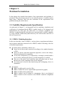
3 Problem Formulation ............................................................................... 15
3.1 Usability Requirements Specification .............................................. 15
3.1.1 PRES+ Modeling Interface ..................................................... 15
3.1.2 PRES+ Simulation Interface ................................................... 16
3.1.3 PRES+ Verification Interface.................................................. 16
3.2 Problem Formulation ........................................................................ 17
4 Related Work............................................................................................. 19
4.1 Petri Net Class Library and Task Modules ....................................... 19
4.2 CTL Formula Parser ......................................................................... 19
4.3 UPPAAL ........................................................................................... 20
5 Tool Design................................................................................................. 21
5.1 GUI Toolkit ....................................................................................... 21
5.2 Overview of the GUIs....................................................................... 21
5.3 Modeling Tool Design ...................................................................... 22
5.3.1 User Interface .......................................................................... 22
5.3.2 Graphical Item Structure ......................................................... 24
5.3.3 Operations ............................................................................... 25
i
5.4
5.5
Simulation Tool Design .................................................................... 36
5.4.1 User Interface .......................................................................... 36
5.4.2 Expand Component Items....................................................... 38
5.4.3 The Token Game ..................................................................... 40
5.4.4 Trace the Simulation ............................................................... 42
5.4.5 Automatic Event...................................................................... 42
Verification Tool Design ................................................................... 43
5.5.1 User Interface .......................................................................... 43
5.5.2 Translate a PRES+ model into a Timed Automata model ...... 45
5.5.3 Parse a query formula into a CTL formula ............................. 46
5.5.4 Translate a CTL formula into a Timed Automata Query ........ 47
5.5.5 Verification.............................................................................. 53
5.5.6 Simulate a diagnostic trace..................................................... 55
6 User Manual .............................................................................................. 57
6.1 Introduction....................................................................................... 57
6.2 Graphical Editor................................................................................ 57
6.2.1 Menu Bar................................................................................. 57
6.2.2 Tool Bar................................................................................... 58
6.2.3 Components List ..................................................................... 58
6.2.4 Items List................................................................................. 58
6.2.5 Drawing................................................................................... 58
6.3 Simulator........................................................................................... 60
6.4 Verifier .............................................................................................. 61
7 Conclusions and Future Work ................................................................. 63
7.1 Conclusions....................................................................................... 63
7.2 Future Work ...................................................................................... 63
Appendix A ...................................................................................................... 65
Appendix B ...................................................................................................... 69
Appendix C ...................................................................................................... 73
References ........................................................................................................ 75
ii
INTRODUCTION
Chapter 1
Introduction
This chapter introduces the motivation and objective of this thesis. Then the
method used in the thesis will be described. Finally, a general view of the
structure of this thesis will be presented.
1.1 Motivation
Embedded systems are currently used in the most diverse contexts from
automobiles and aeronautics to home appliances, medical equipment,
multimedia, and communication devices. With the increment of consumers’
requirements, the embedded systems themselves are becoming more and more
complex. This problem can be solved in design by reusing existing component.
Furthermore, it is of great importance that these systems are correct. For these
reasons, it is necessary to focus on both how to model component-based
embedded systems and how to verify the correctness of them.
PRES+ [4], an extended timed Petri net model, has previously been proposed
to represent component-based embedded systems. The PRES+ model is
simple, intuitive, and can be easily handled by the designer [1].
A tool which integrates modeling, simulation and verification of PRES+
models is therefore desired.
1.2 Objective
The objective of this thesis is to design and implement a design tool which has
the functions for modeling, simulating and verifying PRES+ models
representing component-based systems. And corresponding to each function, a
set of graphical user interfaces (GUIs) is required.
1.3 Method
The work behind the human computer interface, started out with a study of
Petri nets in general [8][9][10], PRES+ [1][3], and the tool Uppaal [7], which
is a similar tool for Timed Automata (TA) [6]. After that user and usability
requirements were defined. The user tasks and objects were then modeled
according to the requirements. Finally the GUI was prototyped and
implemented.
In order to implement the functions, a study of certain background material,
1
CHAPTER 1
such as the Petri Net Class Library [5], was under taken. After this study, data
structures and control flows were identified. In the end, the developed and
implemented functions were integrated with the GUIs.
1.4 Acknowledgements
I especially thank Daniel Karlsson for his great help and patient guidance and
Petru Eles for setting up this master project. I would also like to thank
everyone who has supported me during my work on this master thesis, and all
members of ESLAB for creating a friendly working atmosphere.
1.5 Structure of the paper
The thesis is structured as follows:
Chapter 1 gives a general overview of this thesis, the motivation, the
objective and the method.
Chapter 2 gives some preliminary knowledge on major issues of this
thesis.
Chapter 3 lists the detailed requirements of this thesis.
Chapter 4 presents the related works of this thesis.
Chapter 5 detailed presents the design of each part of this thesis.
Chapter 6 briefly introduces how to use the tool
Chapter 7 summarizes this thesis, and gives the possible future works
2
BACKGROUND
Chapter 2.
Background
In this chapter the necessary theoretical background is presented. First, a brief
introduction of Petri Nets is given, and then a formal definition of PRES+ is
presented. The procedure used for verifying PRES+ relies on the existing tool
UPPAAL. For this reason, PRES+ must be translated into the input language
of UPPAAL, namely Timed Automata. So, timed automata is represented at
the end of this chapter.
2.1 Petri Net
Petri Nets (PNs) were first developed by Carl Adam Petri in his PhD thesis in
1962. With subsequent developments generalizing the Petri Net, and allowing
a wider variety of applications, the Petri Net is now a commonly used tool.
2.1.1 Description
Petri Nets are a modeling tool designed to capture information about the
structure and dynamics of the modeled system. As a graphical and
mathematical modeling tool [9], Petri nets are used to model procedures,
organizations and devices where regulated flows, in particular information
flows, play a role [8]. As a graphical tool, Petri nets can be used as a
visual-communication aid similar to flow charts, block diagrams, and
networks. As a mathematical tool, it is possible to set up state equations,
algebraic equations, and other mathematical models governing the behavior of
systems.
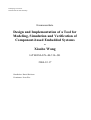
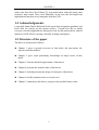
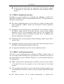
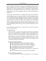
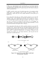
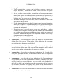
As a special type of graph, a PN is a bipartite directed graph, and consists of
two types of nodes. One is called place, and usually denoted by a circle or an
ellipse (Figure 2.1-a); the other type is called transition, and is usually
denoted by a bar, a square, or a rectangle (Figure 2.1-b). The edges of a PN
are called arcs and are always directed (Figure 2.1-c). As a special property of
a bipartite graph, an edge can connect only nodes that belong to different
types. Therefore, an arc can be from a place to a transition, called Input arc
(Figure 2.1-d), or from a transition to a place, called Output arc (Figure 2.1-e).
In addition to the two types of nodes - places and transitions - and the arcs, a
fourth object is introduced in order to describe the dynamics of a Petri Net.
This object is the token (Figure 2.1-f), denoted by a solid dot, residing inside
the circles representing the places. In classical PNs, however, the tokens do
not represent specific information and are not distinguishable. They are only
used to mark the PN’s state, called marking. A marking, denoted by M, is a
3
CHAPTER 2
map for recording the number of tokens in each place of the PN at a certain
time. Each PN has an initial marking, denoted M0.
a) Place
b) Transition
d) Input Arc
e) Output Arc
c) Arc
f) Token
Figure 2.1 Components of a PN
2.1.2 Mathematical Definition
Formally, a classical PN is a five-tuple N = (P, T, I, O, M0) where
P = {p1, p2, … pm} is a finite non-empty set of places;
T = {t1, t2, … tn} is a finite non-empty set of transitions;
I ⊆ P × T is a finite non-empty set of input arcs, which define the flow
relation between places and transitions;
O ⊆ T × P is a finite non-empty set of output arcs, which define the flow
relation between transitions and places;
M0 is the initial marking of the net. A marking M: P → {0, 1} is a function that
denotes the absence or presence of tokens in the places of the net. M(p) = 1
whenever the place p is marked (contains tokens), otherwise m(p) = 0.
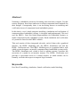
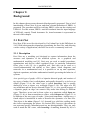
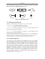
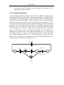
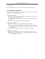
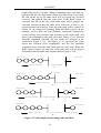
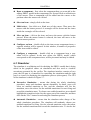
2.1.3 Dynamic Behaviour
The execution of a PN depends on the marking of the net. The marking
records the numbers of tokens in each place of the PN at a certain time. When
there are enough tokens available in the input places of a transition, that is all
the preconditions for the activity are fulfilled, we say the transition is enabled
and can be fired. When the transition fires, it removes tokens from its input
places and adds one token in each of its output places, resulting in another
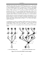
marking. For Example, in Figure 2.2, there is a token in place p0, thus
transition t0 can be fired since there are enough tokens in its input places.
After t0 has fired, the PN reaches a new marking, shown in Figure 2.3 a). In
this new marking, transition t1 is enabled, which when fired leads to the
marking in Figure 2.3 b), Figure 2.3 c).
4
BACKGROUND
t3
p0
t0
p1
t1
p3
t2
p4
t2
p4
t2
p4
p2
Figure 2.2 A simple PN
t3
p0
t0
p1
t1
p3
p2
a)
t3
p0
t0
p1
t1
p2
b)
5
p3
CHAPTER 2
t3
p0
t0
p1
p3
t1
t2
p4
p2
c)
Figure 2.3 Example of the dynamic behaviour of a PN
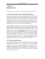
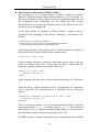
2.2 PRES+
PRES+ (Petri net based Representation for Embedded Systems) [3] is a
computational model based on Petri nets that allows to capture important
features of embedded systems. Since PRES+ is a Petri Net based model, it not
only inherits the characteristics of Petri Nets, but also on top of this, it adds
some special features. For example, PRES+ overcomes the lack of
expressiveness of classical Petri nets where tokens are considered as “black
dots”. In PRES+ tokens hold information that makes it possible to obtain more
succinct representations suitable for practical applications, and when transitions
are fired, the information will be transferred. Moreover, PRES+ can capture
timing aspects by associating lower and upper limits to the duration of
activities related to transitions and keeping time information in token stamps.
Thus the PRES+ is more suitable to represent the real-time embedded system
than classical Petri nets.
[ p 4 − 2]
t3
<4,0>
[2..5]
[ p3 + p 2 ]
[ p1 + 5]
[ p0 ]
[3..4]
p0
[2..5]
t0
p1
[3..7]
t1
p3
[ p3 > p2 × 2]
p2
Figure 2.4 A simple PRES+ model
6
t2
p4
BACKGROUND
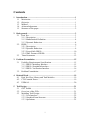
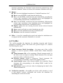
2.2.1 Description
Figure 2.4 presents a simple PRES+ model in Figure 2.4, according to which
we describe the characteristics of PRES+ as follows.
In this PRES+, P={p0, p1, p2, p3, p4} and T={t0, t1, t2, t3}.
As introduced before, tokens carry information. So in PRES+, a token is a
pair k=<v, r> where v is the token value, and this value may be any type. r
is the token time, a non-negative real number representing the time stamp
of the token. In Figure 2.4, the token in place p0 is k=<4, 0>, where the
token value is 4, an integer, and time stamp is 0.
.
In Figure 2.4, this PRES+ is in the initial marking M0, which indicates
place p0 contains a token initially.
Every transition t ∈ T has an associated function and a condition guard.
In addition, timing aspects are captured by the fact that there exists a time
delay interval in each transition.
The function f associated to t has as input arguments the values of the
tokens which are in the input places of the transition t, and the output
of f is found in the values of the tokens that will be in the output
places of t. Transition functions are very important when describing
the behavior of the system to be modeled. They allow systems to be
modeled at different levels of granularity with transitions representing
simple arithmetic operations or complex algorithms. For example, in
Figure 2.4, transition t1 has the function f=p1+5, where p1 means the
value of the token that will appear in place p1, and after t1 fired, the
value of the token in place p3 will be the value of the token in place p1
plus five.
The guard G of a transition t is an important factor to determine if t
can be enabled. In Figure 2.4, transition t2 has a guard G=TRUE if
p3>(p2 × 2) is correct, where p3 and p2 are the values of the tokens in
place p3 and place p2 respectively, or G=FALSE otherwise. And for
other transitions in Figure 2.4, their guards are always TRUE.
The time constraints of a transition t consist of two transition delays,
the minimum transition delay d- and the maximum transition delay d+.
The non-negative real numbers d- and d+ (d- ≤ d+) represent the lower
and upper bounds for the execution time (delay) of the function
associated to the transition. But sometimes some transitions have no
upper bounds, then we denote d+= ∞ or d+=inf, which means that the
transition may not fire. In figure 2.4, the time constrains of transition
t0 is [2..5], where d-=2 and d+=5. The delays give the limits in time
for firing a transition since it becomes enabled, and the actual
7
CHAPTER 2
execution time will be add to the time stamps of the tokens in the
output places of the transition.
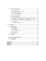
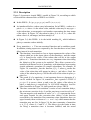
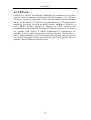
2.2.2 Dynamic Behaviour
Like the dynamic behaviour feature of Petri Nets, in PRES+ model, when a
transition is enabled, it can be fired. A transition t is said to be enabled if all of
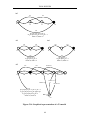
its input places are marked, and its guard is satisfied. Figure 2.5 illustrates the
dynamic behaviour of the PRES+ given in Figure 2.4. In its initial marking,
transition t0 can be fired, and we assume the actual execution time of t0 is 3
time units, between the lower bound 2 and upper bound 5. Then the situation
in Figure 2.5 a) is reached. Now transition t1 is enabled, and can be fired
between 3 and 7. If t1 fires after 5 time units, we obtain the situation in Figure
2.5 b). In Figure 2.5 b), there is a token in place p3 with value 9, and a token in
place p2 with value 4. Since 9 is bigger than double of 4, the guard G of
transition t2 is satisfied and t2 can be fired. Assuming after 3 t2 is fired, then
the tokens in places p2 and p3 are removed, and a new token with value
9+4=13 and time stamp max(3,8)+3=11 will put in place p4, as can be seen in
Figure 2.5 c). Transition t3 is enabled next. A token will appear again in place
p0 after firing t3 at 5 time units in Figure 2.5 d).
[ p 4 − 2]
t3
[ p0 ]
<4,3>
[2..5]
[ p3 + p 2 ]
[ p1 + 5]
[3..4]
p0
[2..5]
t0
p1
[3..7]
t1
<4,3>
p2
a)
8
p3
t2
[ p3 > p 2 × 2]
p4
BACKGROUND
[ p 4 − 2]
t3
[2..5]
[ p1 + 5]
[ p0 ]
<9,8>
[ p3 + p 2 ]
[3..4]
p0
[2..5]
t0
p1
[3..7]
p3
t1
<4,3>
t2
[ p3 > p 2 × 2]
p4
p2
b)
[ p 4 − 2]
t3
[2..5]
[ p 3 + p 2 ] <13,11>
[ p1 + 5]
[ p0 ]
[3..4]
p0
[2..5]
t0
p1
[3..7]
p3
t1
t2
[ p3 > p 2 × 2]
p4
p2
c)
[ p 4 − 2]
t3
<11,16>
[2..5]
[ p3 + p 2 ]
[ p1 + 5]
[ p0 ]
[3..4]
p0
[2..5]
t0
p1
[3..7]
t1
p3
t2
[ p3 > p 2 × 2]
p4
p2
d)
Figure 2.5 Example of the dynamic behaviour of a PRES+
9
CHAPTER 2
2.2.3 Forced Safe PRES+
The bound of a PN is the maximum number of tokens that can reside in a
place in any reachable marking. A PN is said to be safe if the bound is 1. In
this work, we would like to enforce safeness in order to facilitate translation
into Timed Automata. For this reason, the concept in Forced Safe PNs (FSPNs)
is introduced in [1]. In FSPNs, the enabling rule is changed so that, in addition
to the original rules, all output places (except those which are also input places)
must be empty. FSPN can be translated into standard PN in the following way.
If we assume the simple PRES+ model in Figure 2.4 is a forced safe PRES+
model, its equivalent standard PRES+ model is illustrated in Figure 2.6. In the
equivalent standard PRES+ model, each place pi has a duplicated shadow
place ex_pi, and if pi has an initial token, then ex_pi has not and vice versa. In
addition, for each input arc <pi, tj>, there has an output arc <tj, ex_pi>
corresponded. And for each output arc <ti, pj>, there also has an input arc
<ex_pj, ti>.
It is necessary to note that in the rest of this thesis, all models are considered
to be forced safe.
[ p 4 − 2]
t3
ex _ p0
[ p0 ]
<4,3>
ex _ p1
[2..5]
[ p1 + 5]
ex _ p3 [ p 3 + p 2 ]
ex _ p4
[3..4]
p0
[2..5]
[3..7]
t0
p1
t1
p3
t2
[ p3 > p2 × 2]
ex _ p2
p2
Figure 2.6 An equivalent standard PRES+ model of
the forced safe PRES+ model in Figure 2.4
10
p4
BACKGROUND
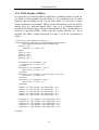
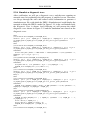
2.2.4 XML Format of PRES+
It is necessary to record the PRES+ model into a standard format. So that, on
one hand, it will minimize the possibility of the translation-user to make
mistakes when building net [5]; On the other hand, it is the base of some
future applications, for example, PRES+ model information could be transfer
among users in a uniform format. XML, since it is a common format of
structured information and a format recommended by W3C, in this thesis, is
selected to represent PRES+ model with the schema PresPlus [5]. As an
example, the PRES+ model illustrated in Figure 2.4 can be represented as
follow:
<?xml version="1.0" encoding="iso-8859-1"?>
<petriNet xmlns:xsi="http://www.w3.org/2001/XMLSchema-instance"
xsi:noNamespaceSchemaLocation='PresPlus.xsd'>
<place id = "p0">
<token time = "0" value = "4"/>
</place>
<place id = "p1"/>
<place id = "p2"/>
<place id = "p3"/>
<place id = "p4"/>
<transition id = "t0" assignment = "p0">
<interval start = "2" stop = "5"/>
</transition>
<transition id = "t1" assignment = "p1+5">
<interval start = "3" stop = "7"/>
</transition>
<transition id = "t2" assignment = "p2+p3" guard = "p3>p2*2">
<interval start = "3" stop = "4"/>
</transition>
<transition id = "t3" assignment = "p4-2">
<interval start = "2" stop = "5"/>
</transition>
<inputArc id = "i01" placeId = "p0" transitionId = "t0"/>
<inputArc id = "i02" placeId = "p1" transitionId = "t1"/>
<inputArc id = "i03" placeId = "p3" transitionId = "t2"/>
<inputArc id = "i04" placeId = "p2" transitionId = "t2"/>
<inputArc id = "i05" placeId = "p4" transitionId = "t3"/>
<outputArc id = "o01" placeId = "p1" transitionId = "t0"/>
<outputArc id = "o02" placeId = "p2" transitionId = "t0"/>
<outputArc id = "o03" placeId = "p3" transitionId = "t1"/>
<outputArc id = "o04" placeId = "p4" transitionId = "t2"/>
<outputArc id = "o05" placeId = "p0" transitionId = "t3"/>
</petriNet>
11
CHAPTER 2
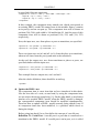
2.3 Timed Automata
The timed automaton model is a labeled transition system model for
components in real-time systems [6]. In this thesis, we use an extended Timed
Automata model (TA) [4] for using existing model checking tool.
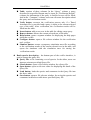
Before we perform the model checking, we need translate a PRES+ model
into a TA model. The detailed translation procedure is represented in [5].
Following we give out the equivalent TA model of the PRES+ model given in
Figure 2.4, and in Figure 2.7 the graph representation of the TA model is
shown.
Note that the PRES+ model must be forced safe PRES+ model when
translated into timed automata for guaranteeing the correctness of the
translation result.
At0
s1
t1?
t1?
t1?
t2?
t2?
t2?
t3?
s2
t3?
t3?
s3
en
t0!
p1:=p0 p2:=p0 p0:=-1
ex_p0:=p0 ex_p1:=-1 ex_p2:=-1
ct0>=2, ct0<=5
At3
At1
t2?
s1
t0?
t2?
t2?
s2
t0?
en
s1
t0?
t2?
s2
t0?
t3!
p0:=p4-2 p4:=-1
ex_p4:=p4-2 ex_p0:=-1
ct3>=2, ct3<=5
t1!
p3:=p1+5 p1:=-1
ex_p1:=p1+5 ex_p3:=-1
ct1>=3, ct1<=7
12
en
BACKGROUND
t0? P3<=p2*2
At2
t0?
t0?
t1?
t1?
t1? P3<=p2*2
t3? P3<=p2*2
s1
t3?
s2
t3?
enc
s3
t1? P3>p2*2
t3? P3>p2*2
t0? P3>p2*2
t2!
p4:=p2+p3 p2:=-1 p3:=-1
ex_p2:=p2+p3 ex_p3:=p2+p3 ex_p4:=-1
ct2>=3, ct2<=4
en
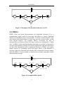
Figure 2.7 An equivalent TA model of
the simple forced safe PRES+ model in Figure 2.4
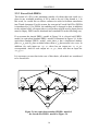
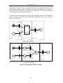
In Figure 2.7, there are four processes At0, At1, At2 and At3, and each process
corresponds to a transition of the PRES+ model, such as At0 is corresponding
to transition t0, At1 to t1, and so on. A process defines the states of a transition
and the shift between two states. Usually we use a circle to denote a state and
use directed arcs to denote the state shifts. The solid circle in the Figure
represents the initial state of the transition. The labels, such as “t0?” And “t0!”,
shared by different automata in the Figure 2.7, are called synchronization
labels. The synchronization labels are used to indicate the synchronization
among processes. For example, in Figure 2.7, transition t0 is enabled. If t0 fires,
process At0 will shift from the state en to s1 via t0!, process At1 will
simultaneously shift from the state s2 to en via t0?, and so on.
Let us examine process At2 corresponding to transition t2. Because t2 has three
input places, including the duplicated shadow place, p2, p3 and ex_p4, t2 will
have four states s1, s2, s3 and en, where s1 means that there are no tokens in
any input place, s2 means that there is only one input place containing a token,
s3 means that there are two input places having tokens, and en means that the
transition is enabled. It is clear in Figure 2.6, the equivalent standard PRES+
of the PRES+ model in Figure 2.4, that only place ex_p4 contains a token, so
the initial state of t2 is s2. In addition, transition t2 has a guard. For this reason,
we use the state enc to specify the situation that all three input places are
having tokens, but the guard of t2 is not satisfied. In order to change a state to
another one, a transition should fire. For instance, if we want shift the state
from At2.s2 to At2.s3, one of the three transitions, t0, t1 and t3, has to fire.
Finally we use “en s1” to describe the firing of this transition.
13
CHAPTER 2
14
PROBLEM FORMULATION
Chapter 3.
Problem Formulation
In this chapter the detailed description of the requirements and problems is
presented. Since the design process is not a linear process, it usually repeats
many times. Therefore, here lists the collection of the requirements and
problems during the whole thesis.
3.1 Usability Requirements Specification
As motivated in chapter 1, an integrated tool for modeling, simulation and
verification of component-based PRES+ models needs to be designed and
implemented. For each part, the main task is to design a graphical user
interface, so that through this interface users can learn how to model, simulate
or verify a PRES+ model easily and effectively. We will describe each GUI of
the tool respectively.
3.1.1 PRES+ Modeling Interface
In this user interface, items of PRES+, such as places, transitions and tokens,
can be drawn, and then connected to be a PRES+ model. Following is the list
of detailed requirements.
For items (places, transitions, tokens, etc.)
Items can be drawn and connected according to the standard notation
of PNs;
Items are shown with their important properties, such as the delays,
function and guard of a transition;
A new item, component [1], is denoted by a rectangle, around which a
set of circles, denoting the ports [1] of the component, is resided;
The size of the place item, transition item and token item are fixed.
But the size of the component item can be changed;
Arc items can be bent so that interleaving and overlapping of arcs is
minimized.
For actions
PRES+ models can be saved to files;
PRES+ model files can be opened and represented in graphs;
PRES+ models can be printed out;
PRES+ models can be loaded as components, that is pre-designed
PRES+ models can be reused in a new PRES+ model as component
items;
15
CHAPTER 3
Actions, such as redo, undo, cut, copy, paste, find and select, should
be designed for improving the efficiency when modeling PRES+
models.
3.1.2 PRES+ Simulation Interface
Simulation is a good method of evaluating and validating a model. The
simulation of PRES+ models is implemented in this GUI. The requirements of
this part are listed below.
The whole simulation process can be shown in a graph. In other words,
when simulating a PRES+ model, the movement of tokens should be
represented;
Simulation can be both interactive and automatic. In an interactive mode,
the PRES+ model will be fired after the user selects which enabled
transition can fire. In an automatic mode, however, the computer will
select an enabled transition randomly, and then fire it. In addition, the
speed of simulation can be adjusted;
Simulation traces can be generated when simulating, and the traces can be
saved to files;
Simulation processes can be traced by steps, and when tracing, the state of
the PRES+ model should match that of the step;
Pre-generated simulation trace files can be loaded and traced.
3.1.3 PRES+ Verification Interface
This GUI is used to implement the verification of PRES+ models. Since we
use an existing model checking tool to perform the verification, the input of
the model checker must be matched. Therefore, several translation functions
are required here.
PRES+ models can be translated into TA models, and for each TA model,
a TA model file can be generated as one of the inputs of the model
checker;
CTL formulas [16], which are used to specify the verification queries, can
be translated into TA terms, in order to serve as another input of the model
checker;
The model checker can be called automatically to perform the
16
PROBLEM FORMULATION
verification;
The verification result can be traced in PRES+ Simulation Interface.
3.2 Problem Formulation
According to the requirements, some problems can be forecast and will be
thought much of when designing the tool.
In PRES+ modeling
How to define the items of the PRES+ model. That is, how to define
the data structure of the items;
How to update a PRES+ model if one or some components inside are
modified;
How to save the graph to a file, and in what format.
In PRES+ simulation
How to simulate into component items of a PRES+ model;
How to connect the simulation trace to the PRES+ model, that is how
to update the state of the PRES+ model based on the step of the
simulation trace;
How to save the simulation trace to a file, and in what format.
In PRES+ verification
How to translate a PRES+ model to a TA model and save it to file;
How to parse the input CTL or TCTL formula, and how to translate
the input formula to TA terms.
17
CHAPTER 3
18
RELATE WORK
Chapter 4.
Related Work
In this chapter, the related work, on which this thesis is based, is presented.
4.1 Petri Net Class Library and Task Modules
The Petri Net Class Library [5] is an extendable Petri net class library. It
defines the data structure of items that belong to Petri Net, the net structure,
the data structure of the state of Petri Nets, and the changes in the net. With
the library, both the users, who use the library, and the implementers, who
extend the library, can build a PN, set initial marking, and simulate a PN easily.
In addition, the Petri Net Class Library provides the analysis interface for the
implementers, but not for users. With the analysis interface, implementers can
read the content of the items and move freely around in the net.
A task module [5] corresponds to a special task, for example the task to
translate a PRES+ model into a Timed Automata model. A PRES+ model
specified with the Petri Net Class Library, can take a module for analysis. That
means the module can use the PRES+ model or the PRES+ model is an input
parameter of the module. Module-implementers can create kinds of task
modules derived from the AbstractModule super class [5] to implement
specific tasks. Many task modules have already been implemented, such as
the Free Choice Module for checking if a PN is free choice, the Strongly
Connectedness Module for checking if a PN is strongly connected, the Make
Safe Module for making a PN safe, the Concurrency Relation Module for
computing the concurrency relation of a PN, the Translation Module for
translating a PRES+ model into a Timed Automata model, and so on.
4.2 CTL Formula Parser
To verify PRES+ models is one of the main parts in this thesis, and we use the
model checking technique for the verification. For model checking,
Computation Tree Logic (CTL) [16] is particular used for specifying the
properties to verify. A class library for defining the data structure of a CTL
formula and translating a query sentence (string) into a CTL formula has been
developed [1]. In this thesis, we will use the library to parse the input query,
build the corresponding data structure, and finally translate the CTL formula
into a Timed Automata query.
19
CHAPTER 4
4.3 UPPAAL
UPPAAL is a toolbox for modeling, simulation and verification of real-time
systems, based on constraint-solving and on-the-fly techniques [17]. UPPAAL
describes a real-time system with a Timed Automata model, and the simulator
and the model-checker of UPPAAL are performed based on Timed Automata
models. In this thesis, we used the model-checker, verifyta, of UPPAAL to
verify PRES+ models. Verifyta is designed to check invariant and
bounded-liveness properties by exploring the symbolic state-space of a system.
For example, with verifyta, if certain combinations of control-nodes are
reachable from an initial configuration could be checked. Verifyta takes as
input a Timed Automata in the textual format and a formula, and a diagnostic
trace will be the output to report the checking results. The diagnostic trace [18]
explains why the formula is satisfied or not.
20
TOOL DESIGIN
Chapter 5.
Tool Design
This chapter presents the whole design process in detail. The whole design
process includes five main parts: GUI toolkit selection, GUI design, modeling
tool design, simulation tool design and verification tool design. Note, since we
have defined a new item, component [1], in PRES+ nets, we use the word
“item” to represent the basic component of PRES+ nets, such as place and
transition. We use the word “component” to represent the new item.
5.1 GUI Toolkit
In this thesis, we design the integrated graphical tool based on the Petri Net
Class Library (see section 4.1) and some task modules [5]. Since the Petri Net
Class Library and the task modules are designed and implemented in C++, we
select to use C++ language in this thesis.
As the main part of this thesis, GUIs need be designed and implemented first.
Usually, when programming a GUI, programmers use a toolkit and follow the
pattern of program design laid down by the toolkit vendor. In this thesis, we
use the Qt toolkit [13]. The Qt toolkit is a C++ class library and a set of tools
for building multiplatform GUI programs using a “write once, compile
anywhere” approach. Qt lets programmers use a single source tree for
applications that will run on multiple operation systems, such as Windows 95
to XP, Linux, Solaris, etc. In addition, Qt provides a powerful mechanism for
seamless object communication and powerful events and event filters, which
make up the C++ Object Model’s inflexible static nature. Consequently, GUI
programming with Qt toolkit is both runtime efficient and flexible [14].
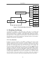
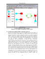
5.2 Overview of the GUIs
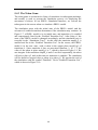
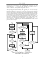
There is a set of graphical user interfaces defined in our design. In Figure 5.1,
some important interfaces are listed and the relationships among these
interfaces are also illustrated. In our design, for each tool, there is a
corresponding main interface. The simulation interface and the verification
interface may be opened from the modeling interface. In addition, the
simulation interface may be opened by the verification interface indirectly.
Therefore, our tool will start with the PRES+ Modeling Interface. The figure
also presents several configuration interfaces which can be produced by the
modeling interface. In the verification interface, an editor may be opened for
browsing files, like TA model files and verification results. We also defined
some other interfaces, such as message windows, for facilitating for users.
21
CHAPTER 5
Configure a
Place
Configure a
Transition
Configure a
Token
PRES+ Modeling Interface
Configure an
Arc
Configure a
Component
Configure
Environment
View TA file
PRES+ Simulation
Interface
PRES+ Verification
Interface
View query
file
View help file
View check
result
Figure 5.1 The Relationships of Interfaces
5.3 Modeling Tool Design
As discussed in chapter 3, the main task of this part is to design and
implement a graphical user interface. Through this interface, users can draw
items and then connect to a PRES+ model. Meanwhile, behind the interface,
the data structure of the graphical items should be consistent with the GUI. In
the following we present the design process from three aspects: user interface,
graphical item structure and operations.
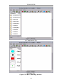
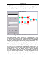
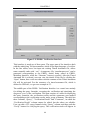
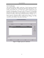
5.3.1 User Interface
In figure 5.2, the user interface of the PRES+ modeling tool is shown. This
interface includes five parts: a menu bar, a toolbar, a toolbox, a canvas and a
status bar. The menu bar consists of five popup menus: File, Edit, View, Tools
and Help. For each popup menu, there are several actions. For example, the
File menu includes the New action for creating a new file, the Open action for
opening an existing file, the Save action for saving the edited PRES+ model,
the Save As action for saving the edited PRES+ model into a specified file,
the Print action for printing the edited PRES+ model and the Exit Action for
exiting from the application. Every action corresponds to a command, which
can be invoked via the menu option. In our design, actions also contain an
icon and a menu text that are represented in popup menus and in the toolbar.
22
TOOL DESIGIN
a ) Components List
b ) Items List
Figure 5.2 PRES+ Modeling Interface
23
CHAPTER 5
The toolbar is a movable panel that contains a set of controls (actions) for
quick access to frequently used commands and options. In the PRES+
Modeling Interface, only one toolbar is created for frequently used commands,
and all these commands correspond to actions in the popup menus.
In the middle of the PRES+ Modeling Interface, there is a splitter widget. The
splitter divides the main part of the interface into two sides. The left side is a
toolbox that contains two list boxes, and the right side is a canvas for
modeling PRES+ models. Toolbox is a widget that displays a column of tabs
one above the other, with the current item displayed below the current tab. In
our design, we build two tabs to put into the toolbox. The two tabs are two list
boxes that list components and items respectively. Items are the basic items of
Petri Nets, which are place, token, transition, arc and nail (a part of arcs for
making arc inflexed, usually denoted with a small circle). Components are
PRES+ models that are already built as reusable IP blocks [1] and exist in the
module library, an appointed directory in the file structure. Canvas provides a
2D area, on which PRES+ models can be drawn.
The status bar, in bottom of the PRES+ Modeling Interface, is a horizontal bar
suitable for displaying status information, such as information of the option
user makes and of the mouse position.
In order to implement the PRES+ Modeling Interface, we first create a main
application window which is derived from the QMainWindow class of Qt.
Then we insert the menu bar, toolbar and status bar into the main application
window. In the third step, we defined our own actions through the abstract
interface provided by QAction class of Qt, and add these actions into menus
and the toolbar. Next, we insert the main part, a splitter widget, into the main
application window. As the left part of the splitter widget, the components list
box is a dynamic list, when the components list is selected the contents of the
list box will be update automatically. And the items list box is a statistic list
with the fixed contents. As the right part, a Qt canvas is put into the splitter
widget, and a view is defined derived from the QCanvasViwe class of Qt to
provide an on-screen view of the canvas.
5.3.2 Graphical Item Structure
Since items are the basic element of PRES+ models, it is necessary to define
the data structure for each item. According to the properties of items, the Petri
Net Class Library [5] gives a general structure for each item. However, in our
design, as graphic objects, items also have some graphical attributes.
Therefore, the data structures of items are re-defined in our tool.
First, in order to be shown on the canvas, items should be canvas items
24
TOOL DESIGIN
defined by Qt. And based on the different shape of items, we use some basic
graph to define them. For example we select QCanvasEllipse class to be
derived for building place and token item, and QCanvasRectangle class for
building transition item. Moreover, for unique identifying items, each item is
arranged a name (Id) when it is constructed and cannot be changed. Second is
to add the general properties to each item’s data structure. For example, the
transition item has two bounds of delay, a guard, an associated function, and
etc. In order to make the graphical PRES+ models more expressive, some
important attributes of items need be shown in the graph. So finally, several
tags with the important information are inserted into the item’s data structure
and these tags are created by deriving from the QCanvasText class.
In our design, there are two complex graphical items. One is arc, and the other
is component. Both of them are an assembled graph. The arc item consists of a
set of lines, a set of nails and an arrow, or an arrow directly. Therefore we
used QCanvasLine class, QCanvasEllipse class, and QCanvasLine class to be
derived for defining line, nail and arrow item respectively, and then combine
them into an arc item. It is necessary to note that the arc item is not a canvas
item. Furthermore, since an arc item contains at least an arrow, we use the
arrow to uniquely identify the arc.
A component item is an abstract representation of a PRES+ model, and we
only focus on its interface [1], but not the detail inside. A component item is
often drawn as a box surrounded by its ports [1], and a port is a kind of place,
denoted by a small circle. So we use QCanvasRectangle class and
QCanvasEllipse class for building a component item.
The detailed items’ data structures are specified in Appendix A.
5.3.3 Operations
Operations are a set of controls that users can operate via the PRES+
Modeling Interface. As introduced in 5.3.1, each control corresponds to an
action. In our design, the controls in PRES+ Modeling Interface can be
divided into two classes. One is the kind of controls that are invoked via a
menu option or a toolbar button, such as Redo and Undo. And the other class
is the kind of controls that are triggered by a set of events. For example, when
a user selects the place item in items list, and clicks the mouse at any position
in the canvas, then the control for drawing a place will be called and a place
will appear at the position where the mouse was clicked. In Table 5.1 all
operations in the PRES+ Modeling Interface are listed.
25
CHAPTER 5
Name
Description
Class
fileNewAction
Create a new file with a blank canvas
1
fileOpenAction
Open a new file
1
fileSaveAction
Save the current model
1
fileSaveAsAction
Save the current model into a specified file
1
filePrintAction
Print the current model
1
fileExitAction
Quit the application
1
editUndoAction
Undo the most recent operation
1
editRedoAction
Redo the most recent undo operation
1
editCutAction
Cut a set of items from canvas (set unvisible)
1
editCopyAction
Copy a set of selected items
1
editPasteAction
Paste a set of copied items to canvas
1
editFindAction
Find an visible item in canvas and select it
1
editSelectAllAction
Select all visible items in canvas
1
viewZoomInAction
Zoom in the canvas
1
viewZoomOutAction
Zoom out the canvas
1
simulationFireAction
Open the current PRES+ net in the simulation window
1
verificationVerifyAction
Open the current PRES+ net in the verification window
1
toolConfigurationAction
Configure the tool
1
toolUpdateAction
Update the current PRES+ net
1
helpContentsAction
Popup the help window with all contents
1
helpIndexAction
Popup the help window with the index
1
helpAboutAction
Messages about the tool
1
ListSelected
Operate if the list is selected
2
LibrarySelected
Operate if the item in components list is selected
2
LibraryHighlighted
Operate if the item in components list is highlighted
2
ComponentSelected
Operate if the item in items list is selected
2
ComponentHighlighted
Operate if the item in items list is highlighted
2
PaintModule
Operate when drawing a component, a place or a transition
2
PaintLine
Operate when drawing a line
2
PaintArrow
Operate when drawing an arrow
2
PaintNail
Operate when drawing a nail
2
PaintIOArc
Operate when drawing an arc
2
PaintToken
Operate when drawing a token
2
MoveItems
Operate when moving an item
2
ReShapeComponent
Operate when re-shaping a component item
2
SelectItems
Operate when selecting an item
2
ConfigureItems
Operate when configuring an item, except component item
2
EditComponents
Operate when editing a component item
2
Table 5.1 Operations List of PRES+ Modeling Interface
26
TOOL DESIGIN
For the controls of the first class, Qt provides many useful objects that can
help to design some actions. For instance, the QFileDialog class provides
dialogs that allow users to traverse their file system in order to select one or
many files or a directory. With this class, we defined our fileOpenAction,
fileSaveAction and fileSaveAsAction easily. But some actions need be
designed based on our own algorithms and rules, such as RedoAction and
UndoAction.
The controls of the second class, are implemented using a major mechanism
of Qt, named meta-object system [13]. The basic idea of this mechanism is to
create independent software components that can be bound together without
any component knowing anything about the other components it is connected
to. As a key service of this mechanism, signals and slots is a fundamental
mechanism used to bind up two objects. For example, in one object, called
sender, a signal is declared, and in the other object, called receiver, a slot is
declared and implemented. When the sender emits the signal, then the receiver
will automatically performs the slot if the slot and the signal have been
connected.
In the following we will describe the solutions for some particular problems
that we met in the design.
Redo and Undo
Redo and Undo are a pair of reverse functions. Undo is the operation that
reverses the last editing action, and Redo restores the last editing action
that was canceled by Undo. Therefore, before designing these two
operations, it is necessary to define the rule to limit the operating scope of
Redo and Undo. The rule here includes two dimensions. One is if the
Undo and Redo operations can be done infinitely? The other is which
action can be Undone or Redone? Below, we list the rule and then present
the mechanism behind Undo and Redo.
The rule of Redo and Undo
Both Undo and Redo can record maximum 10 actions;
The editCutAction operation can be Undone and Redone;
The editPasteAction operation can be Undone and Redone;
The PaintModule operation can be Undone and Redone;
The PaintNail operation can be Undone and Redone;
The PaintIOArc and PaintToken operations can be Undone and
Redone;
The ConfigureItems operation can be Undone and Redone.
The underlying mechanism
We define two stacks to record the undoable edits. The maximum
27
CHAPTER 5
depth of the stacks is 10 units. When an undoable edit is executed, we
push the edit onto the undo stack. When the Undo action is activated,
the edit on the top of the undo stack will be popped up, executed
reversely, and pushed onto the redo stack. If the Redo action is
executed, the edit on the top of the redo stack will be popped up,
executed and moved onto the undo stack. However, if there is any
action executed since the last Undo, the redo stack will be cleared. In
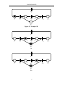
Figure 5.3, an example of operating Undo and Redo is given. In the
example, at first there are four undoable commands (denoted by
circles) having been executed and recorded on the undo stack, and
there is no command in redo stack (shown in Figure 5.3 a)). After an
undoable command executed, the two stacks are changed to the
situation in Figure 5.3 b). The Figure 5.3 c) represents the Undo
action has activated twice sequentially, and the two undoable
commands move from the undo stack onto the redo stack. When the
Redo action executes, the top item of the redo stack will be popped
and pushed onto the undo stack (represented in Figure 5.3 d)).
U n d o s ta c k
R e d o sta c k
H is to ry c o m m a n d
c u rre n t c o m m a n d
a )
e x e c u te d
U n d o s ta c k
R e d o sta c k
H isto ry c o m m a n d
c u rre n t c o m m a n d
b )
U n d o s ta c k
R e d o sta c k
H isto ry c o m m a n d
c u rre n t c o m m a n d
H is to ry c o m m a n d
c )
U n d o sta c k
R e d o s ta c k
H isto ry c o m m a n d
c u rre n t c o m m a n d
H is to ry c o m m a n d
d )
Figure 5.3 An Example of Operating Undo and Redo
28
TOOL DESIGIN
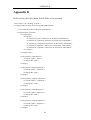
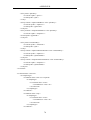
Input format of the graphical PRES+ model
As explained in [5], an input format of PRES+ models is needed.
However, different from the input format defined in [5], in our design, we
add some attributes into the format to specify the graphical properties and
the component items. Meanwhile, we also define the GUI schema
PresGUIPlus.xsd to extend the PresPlus.xsd [5]. The detail of the GUI
schema is given in Appendix B.
In the input format of graphical a PRES+ model, a header must be
specified at the beginning of the format. Following is the detail of the
header.
<?xml version="1.0" encoding="iso-8859-1"?>
<petriNet xmlns:xsi="http://www.w3.org/2001/XMLSchema-instance"
xsi:noNamespaceSchemaLocation='PresGUIPlus.xsd'>
Following the header, all the places are list. We will explain the syntax of
the specification of a place based on the example below.
<place id = "p" x = "100" y = "100"/>
In this example, the place is named p and drawn on the canvas with the
center at position (100, 100). A place can also have a token, and the
following example will show the syntax of this case.
<place id = "p" x = "100" y = "100">
<token time = "0.0" value = "1"/>
</place>
In this example, the place p has a token with the timestamp ‘0.0’ and value
‘1’.
After the places, all the transitions are list. All properties of a transition
will be specified. The specification of a transition has the following
syntax.
<transition id = "t" assignment = "p-1" guard = "p>1" x = "150" y = "150">
<interval start = "0" stop = "2"/>
</transition>
This is a transition named t. It is an output transition of place p with the
associated function f = p – 1, and the guard G = p > 1. The minimum
bound delay of t is ‘0’ and the maximum bound delay is 2. Further more,
the transition’s center is drawn at the position (150, 150).
If a PRES+ model contains component items, all component items should
29
CHAPTER 5
be specified following transitions.
<component id = "com" x = "200" y = "200" width = "100" height = "50">
<inport id = "ip" x = "190" y = "225"/>
<outport id = "op" x = "310" y = "225"/>
</component>
In this example, the component item, named com, which corresponds to
an existing PRES+ model file named com in the module library, contains
an in-port ip and an out-port op. This component item will be drawn at
position (200, 200) with width is 100 and height 50. And the ports of this
component item will be drawn at positions (190, 225) and (310, 225)
respectively.
Next, the input arcs, arcs from places or ports to transitions, are specified.
<inputArc id = "in1" placeId = "p" transitionId = "t"/>
<inputArc id = "in2" portId = "ip" transitionId = "t"/>
These two input arcs are in1 and in2. in1 is from the place p to transition t,
whereas in2 starts from the port ip and ends at the transition t.
At the end, the output arcs, arcs from transitions to places or ports, are
specified similar with the input arcs.
<outputArc id = "out1" placeId = "p" transitionId = "t"/>
<outputArc id = "out2" portId = "op" transitionId = "t"/>
This example lists two output arcs, out1 and out2.
After the whole definition, there should be an end tag.
</petriNet>
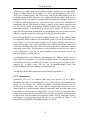
Update the PRES+ net
The component item is a new item that we have introduced in this thesis.
Like the two sides of a coin, on one hand, by using the component item,
we can reduce the design complexity [1]; On the other hand, as an abstract
interface of a reusable PRES+ model, when the PRES+ model is changed,
the corresponded component item should be modified simultaneously.
Therefore how to update a PRES+ model currently being edited if one of
its component items has been modified, is a problem which faced us
during the design.
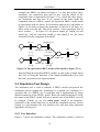
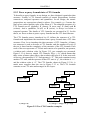
Before going into detail, let us first define the concept of a useful port.
Definition 5.1: Useful Port. A useful port is a port that is connected to a
transition in the PRES+ model. If a useful port is an in-port, so it is called
30
TOOL DESIGIN
a useful in-port. And a useful out-port means that a useful port is an
out-port.
iterator
analyzer
a PRES+ net
a PRES+ net
...
...
a component
item
a component a component
item
item
a component
item
a component
item
a component
item
a component
item
a ) A components tree
a component
item
a component
item
a component
item
b ) Traverse a components tree
Figure 5.4 Tree structure of a PRES+ model
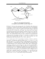
There are two situations in which a PRES+ model needs to be updated.
One is when we open a PRES+ model and the component items inside
have been changed. The other is when a component item of the PRES+
model currently being edited has been modified.
In the first situation, in order to check if the current interface of each
component item is correct, we go through the corresponding PRES+
model to get its correct interface and compare it with the current specified
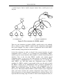
interface. Due to the fact that PRES+ models can contain nested
component items, we can use a tree data structure to represent a PRES+
model, named a component tree. In a component tree, we call the root
node PRES+ net, and other nodes the component items or PRES+
modules. If a PRES+ model is represented in this way, the task to check
the PRES+ model can be implemented with a recursive algorithm for
traversing a components tree. In Figure 5.4, the components tree of a
PRES+ net is presented. Figure 5.4 a) shows that the PRES+ model has
three levels. That means that this PRES+ model contains some component
items, and some of them also contain component items. Figure 5.4 b)
shows the process of traversing the components tree, and the arrows in b)
represent the traversing steps. In order to check each component item, we
31
CHAPTER 5
design an iterator to traverse the component tree. Moreover, we add an
analyzer function into the iterator to check if the interface of each
component item in the tree is correct. For the example in Figure 5.4 b), the
iterator goes through the components tree from the root node, the most
outside PRES+ net, and reaches the most left component item in the
second level. The iterator finds this PRES+ module also contains
component items. Then the iterator goes deeply to the component items in
the third level. Since the PRES+ modules corresponding to the component
items in the third level do not contain any component items, the analyzer
function starts to check the interface of each PRES+ module and returns
back the check result to their father node, the component item in the
second level. The check result can be divided into four classes and for
each class the return value will be 0, 1, 2, or 3 respectively. For the first
class, the return value is 0, which means that the current interface of the
PRES+ module is correct. If the return value equals to 1, the interface of
the PRES+ module has been changed, but all the useful ports of the
interface were not modified. The analyzer function will in this case emit a
warning message to notice the user. If the return value is 2, the interface of
the PRES+ module has been changed, and some of the useful ports of the
interface were modified. The analyzer function will emit a critical
message. In the case that the return value is 3, which means that the
analyzer function cannot parse the input format file of the PRES+ model,
the analyzer function will emit another critical message. In the father node,
the PRES+ module in the second level, if it receives the check result 0, the
iterator will continue to traverse the component tree. If it receives 1, the
input format file of it will be modified and the iterator will continue to
traverse the components tree. And if it receives 2 or 3, it will return the
check result to its father node, the root node of the components tree, and
the iterator will stop to traverse. Finally, if the iterator reaches back to the
root node, the input format file of the PRES+ net will be modified and the
updating process will be finished. It is worthy to note that it is efficient to
model a PRES+ net with some component items, but once any component
items are modified, the updating process of the PRES+ net is
time-consuming. Therefore, it is a trade-off the designers need to think
over before they model a PRES+ net.
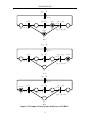
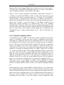
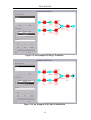
The second situation is not so complex as the first one. When a user
models a PRES+ net with our tool, the user could scan and edit the details
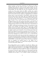
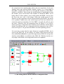
of any component items. In Figure 5.5, an example of updating the editing
PRES+ net is presented. Figure 5.5 a) gives a PRES+ net, and in this net
there is a component item, named tmpM. The interface of tmpM consists
two in-ports, ip1 and ip2, and one out-port, op1. When double clicked the
component item, a new window will pop up to show the details of the
component item (in Figure 5.5 b)). The PRES+ module corresponding to
32
TOOL DESIGIN
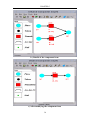
the component item contains three places and two transitions. In the new
window, users may edit the PRES+ module. Figure 5.5 c) is the detail of
the PRES+ module after edited. It is clear that the interface of the PRES+
module is modified. After saving the modifications of tmpM and closing
the window, users can be back to the window in which the PRES+ net is
being edited. In this window, users could update the PRES+ net by click
the icon, the one with a lock image. Since the useful in-port of the
interface of the component item has been modified, the PRES+ net needs
to be updated. Further more, the useful in-port ip2 has been deleted, the
connection between transition t2 of the PRES+ net and ip2 will not exist
any more. Therefore, the old component item (in Figure 5.5 a)) will be
erased, and a new component item with the correct interface will be drawn
instead. In addition, the arcs connected with the component item will be
removed. Figure 5.5 d) presents the PRES+ net after updating process.
It is necessary to note that the input format of a graphical PRES+ net is
saved in an XML file. In our design, we build a class derived from the
class QXmlDefaultHandler to parse the input format XML file and get the
interface of the PRES+ net defined in the XML file. With the interface we
can judge if the PRES+ net being edited needs to be updated.
a ) An editing PRES+ model contains a component item
33
CHAPTER 5
b ) Details of the component item
c ) After modifying the component item
34
TOOL DESIGIN
d ) After updating the PRES+ model
Figure 5.5 An example of updating a PRES+ model
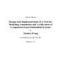
Translate the graphical PRES+ model into Petri Net
The Petri Net Class Library [5] is an extendable Petri net class library. It
defines the structure of the PRES+ net and provides some useful task
modules. Therefore, in order to simplify our tasks, we translate a graphical
PRES+ model into a simple timed Petri Net. To achieve the translation,
we use the interface defined in the SimpleTimedPetriNet class. The class
has the functions createPlace, createTransition, createToken,
createInputArc, and createOutputArc to create the places, transitions,
tokens, input arcs and output arcs respectively. After creating all items of a
simple timed PN, the net will be created spontaneously. With the simple
timed Petri Net model, we can easily simulate the net by calling the
function fire, and translate the net into a TA model by using the task
module, Translation Module. However, the component item of a PRES+
model is not defined in the Petri Net Class Library. When translating, we
have to translate the component item first. In our design, a PRES+ model
may contain several component items and in each component item, there
may also have some component items, like the representation of a
components tree. So we design to expand every component item in every
level of the component tree to the root node level. In other words is to
present all items in every component item in a PRES+ model. For
35
CHAPTER 5
example, the PRES+ net shown in Figure 5.5 a), has three places, three
transitions, one component item and six arcs. And the details of the
component item is represented in Figure 5.5 b), which has three places,
two transitions and four arcs. If we expand all the items inside the
component item to a PRES+ model, the equivalent PRES+ model could
be represented with six places, five transitions and ten arcs, and shown in
Figure 5.6. In order to ensure the uniqueness of the Ids of all items, we
add a prefix to all the Ids. The prefix consists of the component item id
and a symbol “_”. In Figure 5.6, the places tmpM_ip1, tmpM_ip2 and
tmpM_op1, and the transitions tmpM_t1 and tmpM_t2 are the items
extracted from the component item tmpM.
[P1+3]
p1
t1
[2..5]
[tmpM_ip1]
[0]
tmpM_ip1 tmpM_t1
[0..inf]
[P2-3]
[tmpM_ip2]
tmpM_op1
p2
t2
[1..4]
t3
[3..4]
p3
tmpM_ip2 tmpM_t2
[0..inf]
Figure 5.6 The equivalent PRES+ model of the model in Figure 5.5 a)
After building the equivalent PRES+ model, we can create a simple timed
Petri Net by using the functions of the SimpleTimedPetriNet class with
the item’s properties as the input attributes.
5.4 Simulation Tool Design
The simulation tool is used to simulate a PRES+ model and present the
simulation process graphically. Simulation is a method for validating if a
specified state of a PRES+ net is reachable, and is implemented by firing
enabled transitions of the PRES+ model. When an enabled transition is fired,
the tokens in the PRES+ model will move and the state of the PRES+ net will
be changed. Usually we use the token game, which is an interactive
simulation of the model behaviour, to present the simulation process. In this
section, we will introduce the user interface first, and then some important
algorithms will be given.
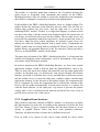
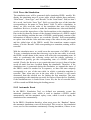
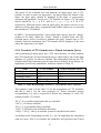
5.4.1 User Interface
Figure 5.7 shows the simulation window. The simulation window is derived
36
TOOL DESIGIN
from QMainWindow class provided by Qt, and consists of two parts. The left
part is a control panel, via which users can simulate a PRES+ model
interactively. The right part is a view, created by deriving from QCanvasView
class, in which the simulation process will be illustrated.
Figure 5.7 PRES+ Simulation Interface
In the control panel, the “Enabled Transition List”, “Simulation Trace”, “Trace
File” and “Control Buttons Group” are widgets enumerated in this order from
top. The part “Enabled Transition List” has a list box, derived from QListBox,
used to list the current enabled transitions ids, and two control buttons, “Fire”
and “Reset”. The “Fire” button is corresponding to firing the transition that
selected in the list box. The “Reset” button is used to reset the marking of the
PRES+ model back to its initial marking. We display the simulation result in a
trace table, which is derived from QTable class, in the part “Simulation Trace”.
The “Trace File” is a line text editor used to display the trace file. In the
“Control Buttons Group”, there are six control buttons and a horizontal slider.
The buttons “Prev”, “Next” and “Replay” are used to trace the simulation
trace. And the buttons “Open” and “Save” are corresponding to operating the
trace file. When the button “Random” is pressed, the simulation will be
performed automatically. During the random simulation, if there are several
enabled transitions at a time, the tool will select an enabled transition
randomly and fire it. In order to adjust the speed of the random simulation, we
37
CHAPTER 5
design a slider, derived from QSlider class, at the bottom of the control panel.
The right part of the PRES+ Simulation Interface, a canvas is provided in
order to display the PRES+ model and the token game.
Figure 5.7 gives out the simulation of the PRES+ model shown in Figure 5.5
a). Before we simulate the PRES+ model, we add a token into place p1, and
the token has the value is 4 and time stamp is 3. In Figure 5.5 a), the PRES+
model contains a component item. But when we simulate the model, we
expand the component item, and for each item inside the component item we
add a prefix, “tmpM_”, to its id. In Figure 5.7, the PRES+ model is in its
initial state, and the transition t1 is enabled and is list in the “Enabled
Transition List”. Therefore, if the “Fire” button is pushed, the transition t1 will
be fired, and the state of the net will be changed, the token will disappear from
place p1 and a token will be appear in place tmpM_ip1. In initial state, the
“Simulation Trace” is empty, and the buttons “Prev”, “Next” and “Replay” are
disabled.
5.4.2 Expand Component Items
As mentioned before, a PRES+ model may contain component items. But,
when it is simulated, tokens may move inside a component item and the
transitions in a component item may be enabled and fired. In order to show
the simulation clearly, therefore, the details of component items are displayed
to users. There are two possible methods to display the contents of component
items. One method is to open a new window to show the details of a
component item when firing a transition inside the component item. Another
method is to expand all component items to a PRES+ model, like in Figure
5.7. In the first solution, there will be many simulation windows open at the
same time, and users need to switch simulation windows frequently. So it is
hard for users to operate simulation and check the simulation results. In
addition, if simulation in this way, it is also hard to us to implement the trace
function. Therefore, we select the second method. However, how to guarantee
there is no any items overlapped after we expand all component items, is a
hard nut to crack. In our design, we make a naïve algorithm to expand
component items of a simple PRES+ model. But for expanding the component
items of a complex PRES+ model, we have not found an intelligent method
yet.
In the following, we give a simple PRES+ model in Figure 5.8 a) to show how
the expanding algorithm works. Firstly we divide the canvas into three areas
based on the left and right borders of the component item tmpM. It is clear
that in area II the component item will be expanded and the right border of
this area will be changed. The items in area I will not be moved after
expanding, and the items in area III should be moved rightwards after
38
TOOL DESIGIN
expanding. In Figure 5.8 b), it presents the three areas after expanding. Like
translating a graphical PRES+ model into a simple timed Petri Net, in order to
ensure all items’ id unique, we add a prefix to all items’ id. The prefix consists
of the component item id and a symbol “_”.
It should be mentioned that for certain complex PRES+ models, this algorithm
may not create nice graphs after expanding component items, but it will not
affect the simulation.
<4,3>
[P1+3]
tmpM_ip1
p1
[0]
tmpM_op1
t1
[2..5]
[P2-3]
t3
[3..4]
tmpM
p3
tmpM_ip2
p2
t2
[1..4]
area I
area II
area III
a) Before Expanding
<4,3>
p1
[P1+3]
t1
[2..5]
[P2-3]
[tmpM _ip1]
[0]
tmpM _ip1 tmpM _t1
[0..inf]
[tmpM _ip2]
tmpM _op1
p2
area I
t2
[1..4]
tmpM _ip2 tmpM _t2
[0..inf]
area II
t3
[3..4]
area III
b) After Expanding
Figure 5.8 Expanding a PRES+ model
39
p3
CHAPTER 5
5.4.3 The Token Game
The token game is an interactive firing of transitions in subsequent markings,
and usually is used to present the simulation process via displaying the
movement of tokens. In our PRES+ Simulation Interface, we execute the
token game in the canvas when we simulate a PRES+ model.
The simulation starts with the initial state of the PRES+ model, and the
existence of enabled transitions determines if the simulation may continue. In
Figure 5.7, a PRES+ model is in its initial state, and transition t1 is enabled
and consequently listed in the “Enabled Transition List”. After firing t1, the
state of the PRES+ model is changed accordingly, and the simulation step is
recorded in the “Simulation Trace”. At this time the transition tmpM_t1 is
enabled and list in the “Enabled Transition List”. In the canvas, the PRES+
model is in the new state, with a token in the output place tmpM_ip1 of
transition t1. Since transition t1 has an associated function f = p1 + 3, the
value of the token in place tmpM_p1 is 7, which is shown in Figure 5.9. We
can imagine if the transitions tmpM_t1 and t3 are fired sequentially, the token
will arrive place p3 and at that time no transition is enabled. The simulation
will be therefore stopped when a token is in place p3. We present the end of
the simulation with the symbol “Deadlock” list in “Enabled Transition List”,
which is shown in Figure 5.10.
40
TOOL DESIGIN
Figure 5.9 An Example of Firing a Transition
Figure 5.10 An Example of the End of Simulation
41
CHAPTER 5
5.4.4 Trace the Simulation
The simulation trace will be generated while simulating PRES+ models. We
display the simulation trace in a trace table, which contains three attributes,
“Item Name”, “Item Type”, and “Results”. In the “Item Name” field, an item’s
id is saved. And in the “Item Type” field, we record the type of the item that
corresponding to the name in “Item Name” field. To trace a simulation, in
theory, we only need the order of the transitions that were fired during
simulation. However, in order to make the simulation trace clear and detailed,
we also record the input places of the fired transitions to the simulation trace.
Due to the fact that the essence of the dynamic behaviour of a PRES+ model
is its state shifting, and that the state of a PRES+ model mainly consists of the
information of tokens in places, we record the “Results” field corresponding
to a place item with the value and time stamp of the token in this place item,
and the global time of the PRES+ model. But transitions cannot contain
tokens, so in the “Results” field corresponding to a transition, nothing will be
recorded.
With the simulation trace, we could recur the movement of a PRES+ model.
To trace a simulation means that when any row in the trace table is selected,
the PRES+ model drawn in the canvas will reflect the corresponding state. In
order to synchronize the selecting action and the redraw operation, a
mechanism to quickly get the corresponding state of a PRES+ model is
needed. Clearly, the fast way to get a particular state is to get it from a list that
saved all states that have occurred during the simulation. Therefore, if the
simulation trace is generated during the simulation, we append the states of
the PRES+ model to another list in sequence, so that each state uniquely
corresponds to a row of the trace table, in which a particular transition is
recorded. Thus, when any row in the trace table is selected, it will search
downward from the selected row for finding the first transition. The state
corresponding to this transition can easily be retrieved from the list. Similarly,
if the simulation trace is loaded from a trace file, the list of recorded states
will be created and filled during the loading process.
5.4.5 Automatic Event
In the PRES+ Simulation Tool, we defined two automatic events: the
automatic simulation event, which is used to simulate a PRES+ model
automatically, and the automatic replay event, which is used to replay the
simulation trace automatically.
In the PRES+ Simulation Interface, when users press the “Random” button,
the automatic simulation event will be invoked. This event is a fast simulation
event, used to fire transitions continuously. During simulation, if there is one
42
TOOL DESIGIN
transition enabled, the transition will be fired. If there are several transitions
enabled at same time, this event will select an enabled transition randomly and
fire it. This automatic event will stop when two situations occur. One situation
is when users press the “Random” button the second time. The other situation
is when there is no enabled transition and the simulation stops. In order to
control the executing speed of this automatic event, we create a slider in the
PRES+ Simulation Interface. Users could drag the slider to set the executing
speed of the automatic simulation event, before they press the “Random”
button.
The automatic replay event can be invoked when users press the “Replay”
button. This event will stop in two situations. One situation is when users
press the “Replay” button the second time. The other is when the tracing
process is at the end of the simulation trace. Similarly as with the automatic
simulation event, users can control the speed of this even via adjusting the
position of the slider in the PRES+ Simulation Interface.
The automatic events are implemented by deriving from timer events. A timer
event is a kind of event that will be fired when the control’s preset timer
interval expires. In the PRES+ Simulation Tool, we start the timer event by
pressing the button, “Random” or “Replay”. The timer interval is connected to
the slider. When the position of the slider is changed, the value of the timer
interval will be modified accordingly.
5.5 Verification Tool Design
The verification tool in this thesis is used to verify a PRES+ model by using
the existing tool verifyta [17].
5.5.1 User Interface
According to the usability requirements specified in chapter 3, the underlying
model checker should be transparent for the user. The verification tool verifyta
may be accessed from UPPAAL’s graphical interface, or in command line. In
our design, we place verifyta behind the PRES+ Verification Interface, and
our program performs the verification via a system call to verifyta. Figure
5.11 shows the PRES+ Verification Interface.
43
CHAPTER 5
Figure 5.11 PRES+ Verification Interface
This interface is made up of three parts. The upper part of the interface deals
with the underlying TA representation, which is the input language of verifyta.
In the line editor, users can input an existing Timed Automata file, whose
name normally ends with “.xta”. A temporary file “translatortext.xta” can be
generated corresponding to the PRES+ model being edited in PRES+
Modeling Interface, when the “Generate” button is pressed. After the Timed
Automata file is selected, user can view the details of the file by clicking the
“Open” button, thus a rich text editor with the contents of the Timed Automata
file will be activated. For the structure of a timed automata file, which is
defined in UPPAAL, we gave an example in 2.3.
The middle part of the PRES+ Verification Interface is a control area mainly
for editing the query formulas, executing the verification and simulating the
diagnostic trace of the verification. This part consists of a table for displaying
the query formulas, the verification results and the comments user marked
corresponding to the verification results, and a group of buttons. The table has
three columns, “Query”, “Verification Result” and “Comment”, in which the
“Verification Result” column cannot be edited, but the others are editable.
User can edit a CTL query formula in the “Query” column, and then push the
“Verify” button for verifying the query. The verification result will appear in
44
TOOL DESIGIN
the “Verification Result” column after verification. Then the user could give
some comments to the result in column “Comment”. Initially, the table is
empty without any rows. If user wants to input a query, the “Insert” button
should be pushed to insert an empty row into the table. Oppositely, when the
“Remove” button is pushed, the currently selected row will be erased from the
table. The “Help” button will give users a brief introduction for how to use the
PRES+ Verification Tool, and the “Configure” button is used to set the path of
the verification tool verifyta. The button, “Simulate”, provides a very useful
function for simulating the diagnostic trace in the PRES+ Simulation
Interface. Sometimes, a verification procedure may go on for quite long times.
For this reason, the “Kill” button is designed for terminating the current
verification process. It is worth to mention that the “Verify” button is disabled
unless there exists a Timed Automata file existent and a query formula input
in the current row of the table. The “Simulate” button will be enabled when a
query is verified.
At the bottom of the PRES+ Verification Interface, the line editor is used to
display an existing query file. A query file encloses a set of query formulas,
and for each formula, there may have a comment. Usually a query file’s name
is end with a suffix “.q”. In this area, there are four control buttons used to
operate the query file. The “Search” button is used to select an existing query
file, the “Open” button is used to open the selected query file in a rich text
editor, the “Load” button is used to parse the query file and load the set of
query formulas into the table above, and the “Save” button is used to save the
queries and comments in the table into a query file. For the structure of a
query file, we will give an example in the Appendix C.
5.5.2 Translate a PRES+ model into a Timed Automata model
When verifying a PRES+ model, we use the available tool, verifyta. Verifyta
is a model checking tool used to verify Timed Automata models. Therefore,
before we make a call to verifyta, we must translate a PRES+ model into a
Timed Automata model. Fortunately, the Petri Net Class Library [5] provides
a task module – Translation Module – to translate a PRES+ model into a
Timed Automata model and save the Timed Automata model into a file. Thus
our task is to translate a graphical PRES+ model into a simple timed Petri Net
model. The translation work is described in section 5.3.3. When we start the
PRES+ Verification Interface, we transfer a PRES+ model to the PRES+
Verification Tool. When the “Generate” button in PRES+ Verification
Interface is pressed, the translation procedure is called to translate the simple
timed Petri Net model into a Timed Automata model and save the Timed
Automata model into a temporary file “translatortext.xta”.
45
CHAPTER 5
5.5.3 Parse a query formula into a CTL formula
To describe a query formula, in our design, we have designed a particular data
structure. Usually a CTL formula consists of atomic propositions, boolean
connectives, temporal operators and quantifiers. In our design, the atomic
propositions are expressions related to places. For example, p==2 means the
place p has a token and the value of the token is 2. The temporal operators of a
CTL formula are G (globally), F (future), X (next step), U (until) and R
(release). And a quantifier, A (all) or E (exists), is always set before a
temporal operator. The details of CTL formulas are presented in [1]. In this
thesis, we focus on how to parse a query formula into the CTL data structure.
The CTL formula parser, introduced in 4.2, defines the structure of a CTL
formula and implements the translation from a query formula into a CTL data
structure. First, let us introduce the data structure of CTL formulas. A binary
tree structure is used to describe a CTL formula, and the number of levels of
the tree is based on the complexity of the structure of the CTL formula. Each
node of the tree represents a CTL unit and consists of a quantifier, an operator,
a relation and a relation value. In Figure 5.12, two examples are presented.
Figure 5.12 a) shows a simple CTL formula, EF(p == 0), which means that
there exists a future where place p has a token with value is 0. In the root node
of the tree, the quantifier is “E” and operator is “F”. This node contains in turn
another CTL unit, and the operator of that CTL unit is “p”, the relation is “==”
and the relation value is “0”. The CTL formula, shown in Figure 5.12 b), is
much more complex than the one in Figure 5.12 a). This CTL formula
contains seven CTL units and arranged in five layers.
[A][G][][]
[E][F][][]
[][->][][]
[][p][==][0]
[A][F][][]
[][p][][]
[][|][][]
[][q][==][0]
[][q][==][1]
b ) AG([p -> AF([q==0 | q==1])])
a ) EF(p==0)
Figure 5.12 Two CTL Formulas examples
46
TOOL DESIGIN
The parser of the available tool can translate an input query into a CTL
formula. In order to parse an input query, the parser limits the format of the
input. An input query should be arranged in the order of propositions,
operators and quantifier. To the two CTL formulas in Figure 5.12, the input
queries should be “0 == p E F” and “p 0 == q 1 == q | A F
A G”
respectively. When the parser catch an input query, the parser traverses every
characters of the input query sequentially and build a binary tree to represent
the translation CTL formula.
In PRES+ Verification Interface, users could input queries into the “Query”
column of the table. When the “Verify” button is pushed down, the CTL
Formula parser will be invoked to translate the query formula into a CTL
formula, and after translation, the CTL formula will be displayed in the area
where the input query was input.
5.5.4 Translate a CTL formula into a Timed Automata Query
After translating an input query into a CTL data structure, we must translate
the CTL formula into a Timed Automata query, which will be one of the input
attributes of verifyta. In order to translate, the relationship between the CTL
formulas and Timed Automata queries must first be defined. In our design, we
implement several basic translations, which are shown in Table 5.2.
Name
CTL Formula
Timed Automata Query
Possibly
EF p
E<> p’
Invariantly
AG p
A[] p’
Potentially always
EG p
E[] p’
Eventually
AF p
A<> p’
Leads to
AG(p -> AF q)
p’ --> q’
Table 5.2 Some Relationships between CTL formulas and TA queries
The symbols p and q in the table 5.2 are the propositions of CTL formulas,
and the p’ and q’ are the state properties of Timed Automata queries
corresponding to p and q respectively. Below the meaning of each CTL
formula in table 5.2 is listed.
“EF p”: it is possible in the future that p is satisfied;
“AG p”: p is always satisfied;
“EG p”: p is potentially always satisfied;
“AF p”: p will always be satisfied in the future;
“AG(p -> AF q)”: once p is satisfied, q must be satisfied in the future.
According to the relationships in table 5.2, we can implement the translation
with two steps. First is to translate the quantifier and operators into Timed
47
CHAPTER 5
Automata queries properties, such as translating “EF” into “E<>”. The second
step is to translate the propositions of CTL formulas into the state properties
of Timed Automata queries, that is to translate p to p’ and q to q’. The symbol
p or q of a CTL formula is an expression of places of a particular PRES+
model. Usually it may be an id of a place, or relations among places. For
example, if the expression is “p”, it means that the place p has a token. And if
the expression is “p == 3”, it means that the value of the token in place p is 3.
Just as its name implies, Timed Automata query is used to describe a Timed
Automata model. Therefore, to translate p to p’ and q to q’, we must translate a
PRES+ model into a Timed Automata model, which is represented in 5.5.2. In
the following we will give an example to illustrate the translation from a
PRES+ model into a Timed Automata model and the translation from a CTL
formula into a Timed Automata query. In Figure 5.13 a), a Forced Safe PRES+
model is illustrated.
As explained in 2.3, before we translate a PRES+ model into a TA model, we
should make the PRES+ model safe. In Figure 5.13 b), it shows the equivalent
standard PRES+ model of the forced safe PRES+ model in Figure 5.13 a).
Figure 5.14 shows the corresponding Timed Automata model of the PRES+
model.
<0,0>
<1,0>
p0
p1
p2
[ p0 ]
[ p1 ]
[ p2 + 3]
t1
t 2 [0..2]
p3
p4
[0..2] t4
[0..2]
p5
<0,0>
<2,0>
ex _ p0 p0
<1,0>
ex _ p1 p1
[ p0 ]
[0..2]
ex _ p5
t4
p5
[0..2]
ex _ p2 p2
[ p1 ]
[ p2 + 3]
t1
t 2 [0..2]
ex _ p3 p3
[ p4 − p3 + p5 ]
[3..6]
<2,0>
ex _ p4
p4
[ p4 − p3 + p5 ]
t3 [ p3 >= 0]
[3..6]
p6
ex _ p6
a ) A Forced Safe PRES+ model
t3 [ p3 >= 0]
p6
b ) An equivalent standard PRES+ model
Figure 5.13 A Forced Safe PRES+ model example
48
TOOL DESIGIN
At2
t3?
s1
t1?
s2
t3?
t1?
t1?
s3
en
t2!
p4:=p2+3 p3:=p2+3 p2:=-1
ex_p2:=p2+3 ex_p3:=-1 ex_p4:=-1
clock>=0, clock<=2
At4
At1
t3?
s1
t3?
t3?
t2?
s2
t2?
t3?
s1
en
en
s2
t4!
p5:=p0 p0:=-1
ex_p0:=p0 ex_p5:=-1
clock>=0, clock<=2
t1!
p3:=p1 p1:=-1
ex_p1:=p1 ex_p3:=-1
clock>=0, clock<=2
At3
t2?
t2?
t1?
s1
t4?
t2? P3<0
t1?
s2
t1?
t4?
s3
t1? P3<0
s4
t4?
t4? P3<0
enc
t1? P3>=0
t2? P3>=0
t4? P3>=0
t3!
p6:=p4-p3+p5 p3:=-1 p4:=-1 p5:=-1
ex_p3:=p4-p3+p5 ex_p4:=p4-p3+p5
ex_p5:=p4-p3+p5 ex_p6:=-1
clock>=3, clock<=6
en
Figure 5.14 Graphical representation of a TA model
49
CHAPTER 5
In the forced safe PRES+ model, if the input query presented in CTL formula
is “EF p3”, which means that a token will possibly reach the place p3 in the
future, the corresponding Timed Automata query should be “E<> p”, where p
is the expression, with an equivalent meaning that there is a token in place p3.
We can split that expression into two parts first, and then connect the two parts
into the whole expression with “or” operator.
The first part states that place p3 must have a token. From the Figure 5.13 a)
and according to the enabling rule of Forced Safe PRES+ models, we can get,
that if transition t3 is enabled or t3 is not enabled only because its guard is not
satisfied, then place p3 must have a token. Therefore, corresponded to the TA
model in Figure 5.14, this part can be written as “At3.en or At3.enc”. In
addition, it is clear that this part is based on the output transitions of place p3.
The second part describes that a token will reach place p3. In Figure 5.13 a),
we can guarantee that a token will arrive at p3 by firing any one of the
transitions t1 and t2. If we fire transition t1, the token in place p1 will move to
place p3 and t1 will be disabled. In this case, according to the TA model in
Figure 5.14, transition t1 is in state s1, denoted by “At1.s1”, and transition t3
may be in state s2, s3, s4, en or enc. So we can use “(At1.s1 and At3.s2) or
(At1.s1 and At3.s3) or (At1.s1 and At3.s4) or (At1.s1 and At3.en) or (At1.s1
and At3.enc)” to describe that a token reach p3 after t1 firing. However, since
“At3.en” and “At3.enc” have been expressed in the first part, we delete the
redundancy and get “(At1.s1 and At3.s2) or (At1.s1 and At3.s3) or (At1.s1
and At3.s4)”. If we fire the transition t2, the token in place p2 will move into
place p3 and place p4 and t2 will be disabled. Same as the t1 firing, in this
case, we can get the description “(At2.s1 and At3.s3) or (At2.s1 and At3.s4)”.
In order to simplify the algorithm, which is used to generate a TA query, we
add a redundant formula into this description and get “(At2.s1 and At3.s2) or
(At2.s1 and At3.s3) or (At2.s1 and At3.s4)”. Therefore the second part of the
expression p is “(At1.s1 and At3.s2) or (At1.s1 and At3.s3) or (At1.s1 and
At3.s4) or (At2.s1 and At3.s2) or (At2.s1 and At3.s3) or (At2.s1 and At3.s4)”.
In addition, it can be seen that this part is based on all transitions connecting
to place p3.
Finally, we connect the two parts to get the whole expression, which is
“At3.en or At3.enc or (At1.s1 and At3.s2) or (At1.s1 and At3.s3) or (At1.s1
and At3.s4) or (At2.s1 and At3.s2) or (At2.s1 and At3.s3) or (At2.s1 and
At3.s4)”
Figure 5.15 presents the flow chart of the algorithm for generating this type of
expressions. The algorithm starts with getting the lists of the input transitions
and the output transitions of the specified place. If the place has output
transitions, the algorithm will deal with the output transitions list to generate
50
TOOL DESIGIN
the first part of the expression and insert it into the expression. For each
output transition ti, if it has a guard, the algorithm will produce “Ati.en or
Ati.enc”. Otherwise, the algorithm will generate “Ati.en”.
After operating all output transitions, the algorithm will deal with the input
transitions of the place to generate the second part of the expression and insert
it into the expression. For each input transition tj, first the algorithm will judge
if tj is an output transition. If tj is an output transition, the algorithm will skip
tj and operate the next input transition (The reason will be explained below).
If tj is not an output transition, the algorithm will calculate the number n of
input places of each output transition ti, which equals to the number of the
states of ti. Then the algorithm the description “(Atj.s1 and Ati.s2) or … or
(Atj.s1 and Ati.sn)”. (That is why we add a redundant formula into the second
part of the above example)
Start
Get the input
transitions list of
the place
If the output transition ti
equals input transition tj
Get the output
transitions list of
the place
If there are output
transitions
Yes
No
No
Get the number n of
input places of each
output transition ti
For each input
transition tj, add
“Atj.synch”into the
expression
Yes
For each output transition ti and
each input transition tj, add
“(Atj.s1 and Ati.s2) or ... or
(Atj.s1 and Ati.sn)” into the
expression
For each output
transition ti, add
“Ati.en”into the
expression
If the transition
ti has guard
No
If all the output
transitions parsed
No
If all the input
transitions parsed
Yes
Yes
Add
“Ati.enc”into the
expression
If all the input
transitions parsed
No
Yes
Yes
No
If all the output
transitions parsed
Yes
End generating
the expression
Figure 5.15 The flow chart of the algorithm for
generating TA query expression
51
No
CHAPTER 5
If there is no output transition of the specified place, for each input transition
tj of the place, the algorithm inserts “Atj.synch” into the expression. Then the
algorithm finishes generating the TA query expression. The reason for this part
will be explained below.
In PRES+ models, a place may be both the input place of a transition and the
output place of the transition, such as place p1 shown in Figure 5.16.
Furthermore, a place may have no any output transitions, such as place p2 in
Figure 5.16.
If we want check if the place p1 will be possibly reached, we give the CTL
formula “EF p1”. After translation, the first part of the TA query is “At1.en”.
And the second part is “(At0.s1 and At1.s2) or (At1.s1 and At1.s2)”, because
t1 is both the input transition and output transition of p1. However “At1.s1
and At1.s2” will never be satisfied. For this reason, in our algorithm, the
logical module “if the output transition ti equals the input transition tj” is used
to exclude this kind of description from a TA query.
If we want check if the place p2 will be possibly reached, we give the CTL
formula “EF p2”. Since p2 does not have any output transitions, both the first
part and the second part of the TA query cannot be generated, and we need
another method to represent that transition t1 fires. In a TA model, we use the
state “synch” to express the firing process of a transition. Therefore, in our
algorithm, the module “For each input transition tj, add Atj.synch into the
expression” is used for this case.
[ p1 + 1]
[ p0 ]
<0,0>
[3..6]
[0..2]
p0
t0
p1
t1
p2
a ) A Forced Safe PRES+ model
At0
At1
t1?
s1
t0?
t1?
s1
en
s2
t0?
s2
t1!
p2:=p1+1 p1:=p1+1
ex_p1:=p1+1 ex_p2:=-1
clock>=3, clock<=6
t0!
p1:=p0 p0:=-1
ex_p0:=p0 ex_p1:=-1
clock>=0, clock<=2
b ) The equivalent TA model
Figure 5.16 A special Forced Safe PRES+ model and
the equivalent TA model
52
en
TOOL DESIGIN
5.5.5 Verification
After having translated a PRES+ model into a Timed Automata model and
saved the TA model into a file, parsed the input query and generate a CTL
formula, and translated the CTL formula into a Timed Automata query and
saved the TA query into a file, we can call verifyta to perform the model
checking. The command line of calling verifyta is “verifyta –s –t 0 [TA model
file] [TA query file]”, and since our verification tool is a graphical tool, the
procedure for calling verifyta will be behind the interface. In Figure 5.17, a
query is input for verifying the PRES+ model shown in Figure 5.5 a), Figure
5.18 shows the situation after the verification, and in Figure 5.19, the
verification result shown in a text editor is presented.
Figure 5.17 Input a query for verification
53
CHAPTER 5
Figure 5.18 After verify the query
Figure 5.19 The verification result
54
TOOL DESIGIN
5.5.6 Simulate a diagnostic trace
After verification, we will get a diagnostic trace, and the trace contains an
example trace for explaining why the property is satisfied or not. Therefore,
we can go through the trace and extract useful information to generate a
simulation trace file, with which the PRES+ Simulation tool could display the
example to debug the PRES+ model. In Figure 5.19, in the verification result,
the diagnostic trace is shown. And following we will present the whole
diagnostic trace shown in Figure 5.19 and the simulation trace based on the
diagnostic trace.
State:
( At1.en At2.s2 At3.s2 AtmpM_t1.s2 AtmpM_t2.s2 )
clock1=0 p2=-1 p3=-1 tmpM_ip1=-1 tmpM_op1=-1 tmpM_ip2=-1 p1=4 ex_p1=-1
ex_tmpM_ip2=0 ex_tmpM_op1=0 ex_tmpM_ip1=0 ex_p3=0 ex_p2=0 syncmutex=0
Delay: 2
State:
( At1.en At2.s2 At3.s2 AtmpM_t1.s2 AtmpM_t2.s2 )
clock1=2 p2=-1 p3=-1 tmpM_ip1=-1 tmpM_op1=-1 tmpM_ip2=-1 p1=4 ex_p1=-1
ex_tmpM_ip2=0 ex_tmpM_op1=0 ex_tmpM_ip1=0 ex_p3=0 ex_p2=0 syncmutex=0
Transitions:
At1.en->At1.synch { clock1 >= 2 && clock1 <= 5 && syncmutex == 0, tau, syncmutex := 1,
tmpM_ip1 := p1 + 3, ex_p1 := p1 + 3 }
State:
( At1.synch At2.s2 At3.s2 AtmpM_t1.s2 AtmpM_t2.s2 )
clock1=2 p2=-1 p3=-1 tmpM_ip1=7 tmpM_op1=-1 tmpM_ip2=-1 p1=4 ex_p1=7
ex_tmpM_ip2=0 ex_tmpM_op1=0 ex_tmpM_ip1=0 ex_p3=0 ex_p2=0 syncmutex=1
Transitions:
At1.synch->At1.s1 { 1, t1!, syncmutex := 0, p1 := -1, ex_tmpM_ip1 := -1 }
AtmpM_t1.s2->AtmpM_t1.en { 1, t1?, clock1 := 0 }
State:
( At1.s1 At2.s2 At3.s2 AtmpM_t1.en AtmpM_t2.s2 )
clock1=0 p2=-1 p3=-1 tmpM_ip1=7 tmpM_op1=-1 tmpM_ip2=-1 p1=-1 ex_p1=7
ex_tmpM_ip2=0 ex_tmpM_op1=0 ex_tmpM_ip1=-1 ex_p3=0 ex_p2=0 syncmutex=0
Delay: 1
State:
( At1.s1 At2.s2 At3.s2 AtmpM_t1.en AtmpM_t2.s2 )
clock1=1 p2=-1 p3=-1 tmpM_ip1=7 tmpM_op1=-1 tmpM_ip2=-1 p1=-1 ex_p1=7
ex_tmpM_ip2=0 ex_tmpM_op1=0 ex_tmpM_ip1=-1 ex_p3=0 ex_p2=0 syncmutex=0
Transitions:
AtmpM_t1.en->AtmpM_t1.synch { clock1 > 0 && syncmutex == 0, tau, syncmutex := 1,
tmpM_op1 := tmpM_ip1, ex_tmpM_ip1 := tmpM_ip1 }
State:
( At1.s1 At2.s2 At3.s2 AtmpM_t1.synch AtmpM_t2.s2 )
clock1=1 p2=-1 p3=-1 tmpM_ip1=7 tmpM_op1=7 tmpM_ip2=-1 p1=-1 ex_p1=7
ex_tmpM_ip2=0 ex_tmpM_op1=0 ex_tmpM_ip1=7 ex_p3=0 ex_p2=0 syncmutex=1
Transitions:
AtmpM_t1.synch->AtmpM_t1.s1 { 1, tmpM_t1!, syncmutex := 0, tmpM_ip1 := -1,
ex_tmpM_op1 := -1 }
At1.s1->At1.s2 { 1, tmpM_t1?, 1 }
At3.s2->At3.en { 1, tmpM_t1?, clock1 := 0 }
AtmpM_t2.s2->AtmpM_t2.s1 { 1, tmpM_t1?, 1 }
State:
( At1.s2 At2.s2 At3.en AtmpM_t1.s1 AtmpM_t2.s1 )
55
CHAPTER 5
clock1=0 p2=-1 p3=-1 tmpM_ip1=-1 tmpM_op1=7 tmpM_ip2=-1 p1=-1
ex_tmpM_ip2=0 ex_tmpM_op1=-1 ex_tmpM_ip1=7 ex_p3=0 ex_p2=0 syncmutex=0
ex_p1=7
In the diagnostic trace, the state and transition expressions appear alternately,
and each state expression presents the state of the TA model and each
transition expression presents the state shift of a particular transition. In
addition, since in TA model, the “At.en
At.synch
At.s1” is used to
present the firing of the transition t, according the diagnostic trace shown
above, we can generate the simulation trace as follow:
[p1]--[place]--[-]--[Value=4, Timestamp=0, Globaltime=0.0.]
[t1]--[transition]--0--[-]
[tmpM_ip1]--[place]--[-]--[Value=7, Timestamp=0, Globaltime=0.0.]
[tmpM_t1]--[transition]--0--[-]
[tmpM_op1]--[place]--[-]--[Value=7, Timestamp=0, Globaltime=0.0.]
This simulation trace means if we fire the transitions t1 and tmpM_t1 in turn,
a token with the value is 7 will reach the place tmpM_op1.
In the PRES+ Verification Interface, when the “Simulate” button is pressed,
the simulation trace file will be generated and the PRES+ Simulation Interface
will be opened with the simulation trace.
56
USER MANUAL
Chapter 6.
User Manual
This chapter represents briefly how to use the tool.
6.1 Introduction
This software is a graphical tool for modeling, simulation and verification of
PRES+ models, and can be run on multiple operation systems, such as
Windows 95 to XP, Linux, Solaris, etc. This graphical tool consists of three
main parts, a graphical editor for modeling PRES+ models, a simulator for
simulating PRES+ models, and a verifier for verifying PRES+ models.
Following we will represent how to use these three parts.
6.2 Graphical Editor
The graphical editor is the main window of this graphical tool, and both the
simulator and verifier could be opened from this editor. The GUI of this editor
is shown in Figure 5.2.
6.2.1 Menu Bar
The menu bar is fixed in the upper of the editor. It contains the following
popup menus.
File – to manage PRES+ model description files
New: re-initiates the editor
Open: loads an existing graphical PRES+ model from file
Save: saves the editing graphical PRES+ model into files
Save As: saves the editing graphical PRES+ model into a specified
files
Print: prints the editing graphical PRES+ model out from printer
Exit: exits this tool
Edit – to control the editions during modeling PRES+ models
Undo: undo the recent operations
Redo: redo the operations that just undone
Cut: deletes a set of selected items and saves them into memory
Copy: saves a set of selected items into memory
Paste: draws items which are in memory on the canvas
Find: finds and selects a specified item
Select All: selects all items on the canvas
57
CHAPTER 6
View – to change the appearance of the editor
Zoom In: magnifies the granularity of the canvas
Zoom Out: shrink the granularity of the canvas
Tool – contains tools to operate PRES+ models
Simulation: invokes and opens the simulator
Verification: invokes and opens the verifier
Update Module: updates a component item of the editing PRES+
model, if the component item has been changed
Configuration: opens a separate window for setting the path of the
modules library and the path of the verification tool, varifyta.
Help – to show the help pages
Contents: opens a separate window for showing the help pages
About: opens a separate window for showing the information about
the version and copyrights of this tool
6.2.2 Tool Bar
The tool bar is normally located just below the menu bar but can be moved to
other positions. The tool bar is divided into four groups, which are
corresponding to the File, Edit, View and Tool popup menu respectively, and
each group provides quick access to some of the most frequently used menu
items.
6.2.3 Components List
The components list, located the leftmost of the main window, lists the names
of the components that exist in the module library. Users can change the
contents of the components list by changing the path of the module library.
6.2.4 Items List
The items list, also located the leftmost of the main window as an alternative
to the components list, fixedly lists the basic items of PRES+ net, such as
place, transition, token, arc and nail.
6.2.5 Drawing
The main function of the graphical editor is to draw a PRES+ model on the
canvas, which is located in the right part of the main window. A PRES+ model
consists of a set of places, a set of tokens, a set of transitions, a set of
components and a set of arcs. And for each arc, it may contain a set of lines, a
set of nails and an arrow.
58
USER MANUAL
Drawing Rules
Tokens must belong to places, and each place contains at most one
token. Therefore, a token can be drawn if there is at least one place
without token on the canvas
An arc, used to connect a place, a transition and a component, can be
drawn from a place to a transition, from a transition to a place, from a
port of a component to a transition, or from a transition to a port. In
addition, there is at most one arc from an item to another item
Nails must belong to arcs. Therefore, a nail can be drawn if there is at
least one arc on the canvas
For the items with same type, the Id (name) of an item must be unique
in a PRES+ model. For a new drawing item, the editor will arrange an
un-replicative id for it, and the id may be modified by users unless
ensuring the uniqueness
Every item may be moved directly except arcs and tokens. A token
could be moved together with the place that contains the token, and an
arc could be moved together with the two items which are connected
by the arc. In addition, the ports of a component could be moved only
along the border of the component
The shape of an item is fixed except components
Draw a place – first select the place item in the items list. Second click on
a blank area of the canvas. Then a place will be added into the canvas at
the position where the mouse was clicked.
Draw a transition – first select the transition item in the items list.
Second click on a blank area of the canvas. Then a transition will be added
into the canvas at the position where the mouse was clicked.
Draw a token – first select the token item in the items list. Second click
on a place, which has no token, on the canvas. Then a token will appear in
the center of the place.
Draw an arc – first select the arc item in the items list. Then starting an
arc by clicking on an item, which should be a place, a transition or a port,
and this item is the source of the arc. For every click on the blank area, a
nail will be added, and a line between the source and a nail, or between
two nails will be drawn too. Finally click should be on another item, a
place, a transition or a port, and this item is the target of the arc.
Draw a nail – first select the nail item in the items list. Second click on an
arc, to which a nail is to be added.
59
CHAPTER 6
Draw a component – first select the component that you want add to the
editing PRES+ model in the components list. Second click on a blank area
of the canvas. Then a component will be added into the canvas at the
position where the mouse was clicked.
Select an item – simply click on the item.
Multi-select – first click on a blank area of the canvas. Then move the
mouse with the button pressed. A rectangle will be drawn and the items
inside the rectangle will be selected.
Move an item – click on the item, and move the mouse with the button
pressed. When the mouse button is released, the item will move to the
current mouse position.
Configure an item – double click on the item except component items, a
separate window will be opened. In this window, a number of properties
of the item could be edited.
Configure a component – double click on a component item, a new
editor will be opened. In the new editor, the PRES+ model, which
corresponds to this component item, will be presented and may be edited.
6.3 Simulator
The simulator is a validation tool for checking the PRES+ model that is being
edited in the graphical editor via simulation and also used to visualize
executions generated by the verifier. The simulator interface consists of two
parts, the left part is a controller for controlling the simulation and the right
part is a viewer for displaying the simulation process (token game). The GUI
of the simulator is shown in Figure 5.7.
Interactive Simulation – means that during the whole simulation
procedure, users and simulator operate alternately. In detail, users will
select an enabled transition to fire, and the simulator will fire the
transition, move the token, list the enabled transitions for next firing and
record the simulation trace. To choose one enabled transition, users should
highlight the transition in the list, the upper part of the controller, and then
click on the “Fire” button for activating the simulator process
Automatic Simulation – means that the simulator takes charge of the
whole simulation procedure. The simulator will randomly choose one
enabled transition for firing, fire the selected transition, move the token,
list the enabled transitions and record the simulation trace. To invoke the
60
USER MANUAL
automatic simulation, the “Random” button should be pushed down. And
when the “Random” button is released, the automatic simulation will stop
Buttons
Fire: fires the highlighted transition in “Enabled Transitions List”.
Reset: resets the PRES+ model into the initial state.
Prev: sets the PRES+ model into the state immediately preceding the
current state according to the simulation trace, and highlights the
corresponding element in the “Simulation Traces”.
Next: sets the PRES+ model into the state immediately following the
current state according to the simulation trace, and highlights the
corresponding element in the “Simulation Traces”.
Replay: replays the trace starting from the current selected element
automatically.
Open: opens and loads an existed simulation trace file.
Save: saves the simulation trace into a simulation file.
Random: starts the automatic simulation.
Slider – is used for controlling the speed used when the simulation trace
is replayed and the automatic simulation is executed
6.4 Verifier
The verifier provides the functions for checking invariant and liveness
properties of a PRES+ model. The verifier GUI, given in Figure 5.11, consists
the following three parts.
Timed Automata Model description – the upper part of the verifier
interface, is used to represent a PRES+ model with a Timed Automata
model.
Timed Automata File: a file containing a Timed Automata model. In
the editor, users can input an existing Timed Automata file as an input
parameter of the verification process.
Generate button: creates a temporary Timed Automata file
corresponding to the PRES+ model in the graphical editor.
Search button: opens a file selector window for a specified Timed
Automata file corresponding to the editing PRES+ model in the
graphical editor.
Open button: opens a rich text editor for displaying the detail of the
Timed Automata file.
Verification controller – the middle part of the verifier interface, is used
to edit queries, execute verification and invoke the simulator for
simulating the verification results.
61
CHAPTER 6
Table: consists of three columns. In the “Query” column, a query
described in a specified format may be input; In “Verification Results”
column, the information if the query is satisfied or not will be filled;
And in the “Comment” column, users can edit some description about
the query and verification results.
Verify button: executes the verification process only if a Timed
Automata file is provided and a query is input to the current selected
row of the table. After verification, the verification results will be
filled into the table.
Insert button: adds a new row in the table for editing a new query.
Remove button: deletes the current selected row of the table.
Help button: opens a separate window for displaying the help pages
about the verifier.
Configure button: opens a file selector window for the verification
tool, verifyta.
Simulate button: creates a temporary simulation trace file according
to the verification results of the current selected row in the table, and
opens the simulator with the simulation trace for tracing the
verification results.
Batch queries description – the bottom part of the verifier interface, is
used to operate the query file.
Query File: a file containing a set of queries. In the editor, users can
input an existent pre-edited Query file.
Search button: opens a file selector window for a Query file.
Open button: opens a rich text editor for displaying the detail of the
Query file.
Load button: loads the queries and comments in the Query file into
the above table.
Save button: opens a file selector window for saving the queries and
comments in the above table into a specified Query file.
62
CONCLUSIONS AND FUTURE WORK
Chapter 7.
Conclusions and Future Work
This chapter presents a summary of this thesis, and also points out some
interesting future works.
7.1 Conclusions
In this thesis, an implementation of an integrated graphical tool for modeling,
simulation and verification of PRES+ models has been presented. PRES+ is
an extended timed Petri Net model used to represent the embedded systems.
The designers and analyzers of component-based embedded systems could
use this tool when they build and check a system.
This tool consists of three main sub-tools, PRES+ modeling tool, PRES+
simulation tool and PRES+ verification tool. By using the PRES+ modeling
tool, users can create PRES+ models and design the properties of each item in
PRES+ models. In addition, we introduced the component item, which is an
abstract interface of a pre-edited PRES+ model, in PRES+ models so that it
becomes simpler and more efficient to build a big and complex PRES+ model.
We also defined an input format of a graphical PRES+ model, which is
presented in XML with the graphical attributes.
The PRES+ simulation tool provides a way to validate PRES+ models. With
this sub tool, users can simulate PRES+ models interactively or automatically.
During the simulation, the simulating process is visualized via displaying the
token game, and can be traced from the simulation trace.
The PRES+ verification tool is used to check invariant and liveness properties
of PRES+ models. Two inputs are needed for the verification process, one is a
query formula, and the other is a Timed Automata model. A particular CTL
data structure is selected to describe the query. The second input, a textural
format file of a Timed Automata model is used, which may be generated
automatically by translating a PRES+ model into a Timed Automata model.
The verification result will be presented in the GUI of this sub-tool, and may
be validated by the PRES+ simulation tool.
7.2 Future Work
The main contribution of this thesis is to implement an integrated graphical
tool for modeling and analyzing component-based embedded systems. Future
work could be aimed to improve the usability of this tool and make better the
63
CHAPTER 7
GUIs of this tool.
This tool includes the fundamental functions for modeling, simulating and
verifying PRES+ models. Improvements may be found in each part. For
example, for the PRES+ modeling tool, a better Undo and Redo rule is
necessary to be defined for making the modeling process more efficient. For
the PRES+ simulation tool, a better algorithm needs to be found for expanding
the component items of a PRES+ model. And for the PRES+ verification tool,
the parser for analyzing the CTL formula can only recognize the postfix
formulas. Therefore, it is better if a new parser could be designed for
recognizing the normal CTL formulas directly.
The GUIs of this tool are designed mainly based on the functionalities of the
tool. So the improvers could think more about the end-users’ feeling on these
GUIs.
64
APPENDIX A
Appendix A
In this section, the definition of each graphical item is presented.
Place Item
PlaceItem class, derived from QCanvasEllipse, provides an interface of a
graphical place.
QPtrList<ArcItem> inList;
QPtrList<ArcItem> outList;
int selfno;
static int placenum;
QString tagtext;
TagItem *tag;
TokenItem *token;
bool visible;
bool selectflag;
//input arcs list
//output arcs list
//the no. of a place
//the unique no. of places
//the ID (name) of a place
//the tag item to show the ID (name) of a place
//the token item of a place, initially equals 0
//if a place is visible, true is visible and false is unvisible.
//if a place is selected, true is selected and false is
unselected.
Transition Item
TransitionItem class, derived from QCanvasRectangle, provides an interface
of a graphical transition.
QPtrList<ArcItem> inList;
QPtrList<ArcItem> outList;
int selfno;
static int transitionnum;
QString tagtext;
TagItem *tag;
TagItem *tag1;
TagItem *tag2;
QString lowerBound;
QString upperBound;
QString triggerTime;
QString firingTimeProposal;
QString assignment;
QString guard;
bool guardExists;
bool infinite;
bool visible;
bool selectflag;
//input arcs list
//output arcs list
//the no. of a transition
//the unique no. of transitions
//the ID (name) of a transition
//the tag item to show the ID (name) of a transition
//the tag item to show the delays of a transition
//the tag item to show the assignment of a transition
//the minimum delay of a transition
//the maximum delay of a transition
//the trigger time of a transition
//the firing time proposal of a transition
//the associated function of a transition
//the guard of a transition
//if a transition has a guard
//if a transition has the maximum delay
//if a transition is visible
//if a transition is selected
65
APPENDIX A
Token Item
TokenItem class, derived from QCanvasEllipse, provides an interface of a
graphical token.
QcanvasItem *fatherplace;
int selfno;
static int tokennum;
QString value;
QString timestamp;
TagItem *tag;
bool visible;
bool fatherisplace;
//the (place or port) item that contains the token
//the no. of a token
//the unique no. of tokens
//the value of a token
//the timestamp of a token
//the tag item to show the value and a timestamp of a token
//if a token is visible
//if the item that contains the token is a place
Port Item
PortItem class, derived from QCanvasEllipse, provides an interface of a
graphical port.
QPtrList<ArcItem> inList;
QPtrList<ArcItem> outList;
TagItem *tag;
TagItem *tag1;
TokenItem *token;
ComponentItem *fatherbox;
bool porttype;
bool visible;
bool selectflag;
//input arcs list
//output arcs list
//the tag item to show the ID (name) of a port
//the tag item to show the type of a port
//the token item of the port, initially equals 0
//the component item that contains the port
//if the port is an input port
//if the port is visible
//if the port is selected
Component Item
ComponentItem class, derived from QCanvasRectangle, provides an interface
of a graphical component.
QCanvasItemList inportlist;
QCanvasItemList outportlist;
TagItem *tag;
bool visible;
bool selectflag;
//in-ports list
//out-ports list
//the tag item to show the name of a component
//if the component is visible
//if the component is selected
66
APPENDIX A
Line Item
LineItem class, derived from QCanvasLine, provides an interface of a
graphical line, a part of an arc.
QCanvasItem *fromitem;
QCanvasItem *toitem;
ArcItem *fatherarc;
int connecttype;
bool visible;
//one item that the line connected
//the other item that the line connected
//the arc that contains the line
//the type of the line according to the items it connected. 0
means from a nail to a nail, 1 means from a place to a nail,
2 means from a port to a nail, and 3 means from a
transition to a nail
//if the line is visible
Arrow Item
ArrowItem class, derived from QCanvasLine, provides an interface of a
graphical arrow, a part of an arc.
QCanvasItem *fromitem;
QCanvasItem *toitem;
ArcItem *fatherarc;
QCanvasLine *arrowline1;
QCanvasLine *arrowline2;
int connecttype;
bool visible;
//one item that the arrow connected
//the other item that the arrow connected
//the arc that contains the arrow
//used for drawing the arrow
//used for drawing the arrow
//the type of the arrow according to the items it connected.
0 means from a nail to a place, 1 means from a nail to a
transition, 2 means from a nail to a port, 3 means from a
place to a transition, 4 means from a transition to a place,
5 means from a port to a transition, and 6 means from a
transition to a port.
//if the arrow is visible
Nail Item
NailItem class, derived from QCanvasEllipse, provides an interface of a
graphical nail, a part of an arc.
QCanvasItem *prelink;
QCanvasItem *nextlink;
QCanvasItem *preitem;
QCanvasItem *nextitem;
ArcItem *fatherarc;
bool visible;
//one link that the nail is connected
//the other link that the nail is connected
//the other item the prelink is connected
//the other item the nextlink is connected
//the arc that contains the nail
//if the nail is visible
67
APPENDIX A
Arc Item
ArcItem class provides an interface of a graphical arc.
QCanvasItem *fromitem;
QCanvasItem *toitem;
int selfno;
static int arcnum;
QString tagtext;
TagItem *tag;
QPtrList<NailItem> nailList;
ArrowItem *arrowitem;
int connecttype;
bool visible;
bool selectflag;
//one item that the arc connected
//the other item that the arc connected
//the no. of an arc
//the unique no. of arcs
//the ID (name) of an arc
//the tag item to show the ID (name) of an arc
//the nails list
//the arrow that the arc contains
//the type of the arc according to the items it connected. 0
means from a place to a transition, 1 means from a
transition to a place, 2 means from a port to a transition,
and 3 means from a transition to a port.
//if the arc is visible
//if the arc is selected
68
APPENDIX B
Appendix B
In this section, the GUI schema PresGUIPlus.xsd is presented.
<?xml version="1.0" encoding="UTF-8"?>
<xs:schema xmlns:xs='http://www.w3.org/2001/XMLSchema'>
<!-- Here starts the content of the petri net definition.-->
<xs:element name="petriNet">
<xs:complexType>
<xs:sequence>
<xs:element ref="place" minOccurs='0' maxOccurs='unbounded'/>
<xs:element ref="transition" minOccurs='0' maxOccurs='unbounded'/>
<xs:element ref="component" minOccurs='0' maxOccurs='unbounded'/>
<xs:element ref="inputArc" minOccurs='0' maxOccurs='unbounded'/>
<xs:element ref="outputArc" minOccurs='0' maxOccurs='unbounded'/>
</xs:sequence>
</xs:complexType>
<xs:unique name="uniquePlaces">
<xs:selector xpath="./place"/>
<xs:field xpath="@id"/>
</xs:unique>
<xs:unique name="uniqueTransitions">
<xs:selector xpath="./transition"/>
<xs:field xpath="@id"/>
</xs:unique>
<xs:unique name="uniqueComponents">
<xs:selector xpath="./component"/>
<xs:field xpath="@id"/>
</xs:unique>
<xs:unique name="uniqueInputArcs">
<xs:selector xpath="./inputArcs"/>
<xs:field xpath="@id"/>
</xs:unique>
<xs:unique name="uniqueOutputArcs">
<xs:selector xpath="./outputArc"/>
<xs:field xpath="@id"/>
</xs:unique>
69
APPENDIX B
<xs:key name='placeKey'>
<xs:selector xpath="./place"/>
<xs:field xpath="@id"/>
</xs:key>
<xs:keyref name="inputArcRefPlaces" refer='placeKey'>
<xs:selector xpath="./inputArc"/>
<xs:field xpath="@placeId"/>
</xs:keyref>
<xs:keyref name="outputArcRefPlaces" refer='placeKey'>
<xs:selector xpath="./outputArc"/>
<xs:field xpath="@placeId"/>
</xs:keyref>
<xs:key name='transitionKey'>
<xs:selector xpath="./transition"/>
<xs:field xpath="@id"/>
</xs:key>
<xs:keyref name="inputArcReferTransitions" refer='transitionKey'>
<xs:selector xpath="./inputArc"/>
<xs:field xpath="@transitionId"/>
</xs:keyref>
<xs:keyref name="outputArcReferTransitions" refer='transitionKey'>
<xs:selector xpath="./outputArc"/>
<xs:field xpath="@transitionId"/>
</xs:keyref>
</xs:element>
<xs:element name="interval">
<xs:complexType>
<xs:attribute name="start" use='required'>
<xs:simpleType>
<xs:restriction base='xs:int'>
<xs:minInclusive value="0"/>
</xs:restriction>
</xs:simpleType>
</xs:attribute>
<xs:attribute name="stop">
<xs:simpleType>
<xs:restriction base='xs:int'>
<xs:minInclusive value="0"/>
</xs:restriction>
</xs:simpleType>
</xs:attribute>
70
APPENDIX B
</xs:complexType>
</xs:element>
<xs:element name="token">
<xs:complexType>
<xs:attribute name="time" use='required'>
<xs:simpleType>
<xs:restriction base='xs:decimal'>
<xs:minInclusive value="0"/>
</xs:restriction>
</xs:simpleType>
</xs:attribute>
<xs:attribute type='xs:int' name="value" use='required'/>
</xs:complexType>
</xs:element>
<xs:element name="inport">
<xs:complexType>
<xs:attribute name="id" type="xs:ID" use='required'/>
</xs:complexType>
</xs:element>
<xs:element name="outport">
<xs:complexType>
<xs:attribute name="id" type="xs:ID" use='required'/>
</xs:complexType>
</xs:element>
<xs:element name="place">
<xs:complexType>
<xs:all>
<xs:element ref="token" minOccurs='0' maxOccurs='1'/>
</xs:all>
<xs:attribute name="id" type="xs:ID" use='required'/>
<xs:attribute name="x" type='xs:string' use='required'/>
<xs:attribute name="y" type='xs:string' use='required'/>
</xs:complexType>
</xs:element>
<xs:element name="transition">
<xs:complexType>
<xs:all>
<xs:element ref="interval"/>
</xs:all>
71
APPENDIX B
<xs:attribute name="id" type="xs:ID" use='required'/>
<xs:attribute name="x" type='xs:string' use='required'/>
<xs:attribute name="y" type='xs:string' use='required'/>
<xs:attribute name="assignment" type='xs:string' use='required'/>
<xs:attribute name="guard" type='xs:string' use='optional'/>
</xs:complexType>
</xs:element>
<xs:element name="component">
<xs:complexType>
<xs:all>
<xs:element ref="inport"/>
<xs:element ref="outport"/>
</xs:all>
<xs:attribute name="id" type="xs:ID" use='required'/>
<xs:attribute name="x" type='xs:string' use='required'/>
<xs:attribute name="y" type='xs:string' use='required'/>
<xs:attribute name="width" type='xs:string' use='required'/>
<xs:attribute name="height" type='xs:string' use='required'/>
</xs:complexType>
</xs:element>
<xs:element name="inputArc">
<xs:complexType>
<xs:attribute name="id" type="xs:ID" use='required'/>
<xs:attribute name="placeId" type="xs:IDREF" use='optional'/>
<xs:attribute name="portId" type="xs:IDREF" use='optional'/>
<xs:attribute name="transitionId" type="xs:IDREF" use='required'/>
</xs:complexType>
</xs:element>
<xs:element name="outputArc">
<xs:complexType>
<xs:attribute name="id" type="xs:ID" use='required'/>
<xs:attribute name="placeId" type="xs:IDREF" use='optional'/>
<xs:attribute name="portId" type="xs:IDREF" use='optional'/>
<xs:attribute name="transitionId" type="xs:IDREF" use='required'/>
</xs:complexType>
</xs:element>
</xs:schema>
72
APPENDIX C
Appendix C
In this section, an example is presented for giving out the structure of an input
query file.
Following is the contents of an input query file for verifying the PRES+ net
shown in Figure 5.13 a).
/*
* EF(p3) - in the future, a token will possibly reach p3.
*/
p3 E F
/*
* AG(p3->EF(p6)) - once a token reaches p3, then a token will possibly reach p6 in the future.
*/
p3 p6 E F -> A G
73
APPENDIX C
74
REFERENCES
References
[1]
[2]
[3]
[4]
[5]
[6]
[7]
[8]
[9]
[10]
[11]
[12]
[13]
[14]
[15]
[16]
Daniel Karlsson, “Towards Formal Verification in a Component-based
Reuse Methodology.” Licentiate Thesis No. 1058, Dept. of Computer
and Information Science, Linköping University, December 2003.
Daniel Karlsson, Petru Eles, Zebo Peng, “A Front End to a Java Based
Environment for the Design of Embedded Systems,” in 4th IEEE
DDECS Workshop, Gyor, Hungary, April 2001, pp. 71-78.
L.A. Cortes, “A Petri Net based Modeling and Verification Technique
for Real-Time Embedded Systems.” Licentiate Thesis No. 919, Dept. of
Computer and Information Science, Linköping University, December
2001.
L.A. Cortes, Petru Eles, Zebo Peng, “Verification of Real-Time
Embedded Systems using Petri Nets Models and Timed Automata,” in
8th International Conference on Real-Time Computing Systems and
Applications (RTCSA 2002), Tokyo, Japan, March 18-20, 2002, pp.
191-199.
Henrik Friman, “Petri Net Class Library and Translation from PRES+ to
Timed Automata.” Master Thesis, Dept. of Computer and Information
Science, Linköping University, December 2003.
R. Alur, “Timed Automata”, in Computer-Aided Verification, LNCS
1633, Berlin: Springer-Verlag, 1999, pp. 8-22.
Collaboration between the Basic Research in Computer Science at
Aalborg University (AAL) and the Department of Computer Systems
(DoCS) at Uppsala University (UPP), http://www.uppaal.com/.
W. Reisig, “Petri Nets: An Introduction.” Springer-Verlag, Berlin,
Heidelberg, New York, Tokyo
J. Desel and J. Esparza, “Free Choice Petri Nets.” Cambridge University
Press, Cambridge, 1995.
Peterson, James L., “Petri Net Theory and the Modeling of Systems,”
Prentice Hall, Englewood Cliffs, NJ, 1981.
Sergio Yovine, “Model Checking Timed Automata,” Verimag Centre
Equation 2, Av. De Vignate 38610 Gieres, France.
Overview of existing tools for Petri Nets, Petri Nets World,
http://www.daimi.au.dk/PetriNets/tools/quick.html
Jasmin Blanchette, Mark Summerfield, “C++ GUI Programming with
Qt3,” Prentice Hall in association with Trolltech Press, published by
Pearson Education, Inc.
“Qt
Reference
Documentation.”
http://www.trolltech.com/documentation
Bruce Eckel, “Thinking in C++,” published by Prentice Hall in 1999.
E.M. Clarke, E.A. Emerson, A.P. Sistla, “Automatic Verification of
Finite-State Concurrent Systems Using Temporal Logic Specifications,”
75
REFERENCES
in Transactions on Programming Languages and Systems, PP.
8(2):244-263, 1986
[17] Kim G. Larsen, Paul Pettersson, and Wang Yi, “UPPAAL in a Nutshell.”
Department of Computer Science and Mathematics, Aalborg University,
Denmark. Department of Computer Systems, Uppsala University,
Sweden.
[18] Kim G. Larsen, Paul Pettersson, and Wang Yi, “Diagnostic
Model-Checking for Real-Time Systems,” in Proc. of Workshop on
Verification and Control of Hybrid Systems III, volume 1066 of Lecture
Notes in Computer Science, pages 575-586. Springer-Verlag, October
1995.
76