1
CENTER FOR
MACHINE PERCEPTION
Reference Tracking System for a
Mobile Skid Steer Robot
CZECH TECHNICAL
(Version 1.20)
UNIVERSITY IN PRAGUE
Vladimı́r Kubelka, Vladimı́r Burian,
Přemysl Kafka
[email protected]
USER MANUAL
May 9, 2012
Available at
https://cw.felk.cvut.cz/doku.php/misc/projects/nifti/sw/start
Center for Machine Perception, Department of Cybernetics
Faculty of Electrical Engineering, Czech Technical University
Technická 2, 166 27 Prague 6, Czech Republic
fax +420 2 2435 7385, phone +420 2 2435 7637, www: http://cmp.felk.cvut.cz
Reference Tracking System for a Mobile Skid
Steer Robot
Vladimı́r Kubelka, Vladimı́r Burian, Přemysl Kafka
May 9, 2012
Abstract
The reference tracking system was developed for the NiFTI robot
odometry system performance verification as a ”Prace v tymu a jeji organizace A3M99PTO” course semester project. It uses a single video
camera to track the robot movement in a plane. A distinct colored
marker must be attached to the robot to be tracked. The tracker
can also determine the robot azimuth given the target contains two
differently colored areas. This report serves as a user manual demonstrating the system usage and will lead the reader through the entire
process.
1
Contents
1 Introduction
2 The
2.1
2.2
2.3
2.4
experiment
The experimental setup . . .
The calibration . . . . . . .
The robot odometry system
The experiment . . . . . . .
3
.
.
.
.
3
3
4
4
6
3 The tracking software part
3.1 The software prerequisites and outputs . . . . . . . . . . . . .
3.2 Step-by-step instructions . . . . . . . . . . . . . . . . . . . . .
8
8
8
.
.
.
.
2
.
.
.
.
.
.
.
.
.
.
.
.
.
.
.
.
.
.
.
.
.
.
.
.
.
.
.
.
.
.
.
.
.
.
.
.
.
.
.
.
.
.
.
.
.
.
.
.
.
.
.
.
.
.
.
.
.
.
.
.
.
.
.
.
.
.
.
.
1
Introduction
The aim of the project was to design and create a video camera reference
tracking system. The system would determine position and heading of a
mobile robot using image processing methods. The specifications were:
• an easy-to-install camera setup
• usable outdoor, independent on light conditions
• supporting the robot odometry system including synchronization
All the specifications were fulfilled reaching localization accuracy (15 ± 13)
cm and heading accuracy (3.8 ± 2.7) degrees (the heading accuracy depends
on the robot distance, the position accuracy applies for the whole experiment
area).
2
The experiment
2.1
The experimental setup
Before describing the experiment setup steps, this is a necessary equipment
list:
• video camera
• stable tripod or equivalent camera support
• measuring tape
• paper sticks (to mark a certain point on the ground)
• colored target (will be described)
The robot must be equipped with a colored target (Fig. 1 or 2 or similar,
the color is arbitrary, but unique in the scene). Since the experiment will
be recorded using a video camera probably not positioned directly above the
robot (ideal setup), the target should be visible from any direction from a
certain height above it (recording from a second floor window has been found
sufficient).
The video camera, as mentioned before, should be positioned as high as
possible. It must have the whole experiment scene in its view and must not
be moved after the calibration points were recorded. We recommend some
heavy-duty tripod.
3
Figure 1: A simple 2D tracking target.
2.2
The calibration
To transform the tracked image data into the world coordinates, a set of
at least 4 points must be recorded. A short video (several seconds) - NOT
a photograph - of the robot standing on each calibration point should be
recorded. World coordinates of the calibration points must be known, thus,
some measuring tape, paper and pencil is required. It is suitable to create
some solid marks at the experimental area to save some time.
IMPORTANT: There must be at least 4 calibration points of which any
3 must not lay in a line - for example, a square fulfills this condition. Having
these 4 points, other may be added to increase the homography transformation accuracy. The calibration points should cover the whole experiment
area.
2.3
The robot odometry system
The reference system can be used for other purposes, but the original one
is performance verification and tuning of the robot odometry system. Also,
4
Figure 2: A 2D + azimuth tracking target.
the reference system expects one of the log files created by the odometry
system to be provided. The steps to launch the robot odometry system are
as follows:
1. Turn the robot on.
2. Log in using a ssh shell connection.
3. Launch the basic set of nodes by typing ”roslaunch nifti drivers launchers
ugv.launch”
4. Verify the logging of the odometry data is enabled by checking the appropriate value in the ”nifti vision/inso/launch/inso.launch” file. Make
sure the logging into the ”vpa” file is enabled:
<param name="inso_vpa" value="$(find inso)/logger/inso_vpa" />
<param name="inso_logging" value="true" />
5. Launch the odometry system: ”roslaunch inso inso.lauch”
5
6. Wait until the ”Calibration finished” message appears before moving
the robot.
Every time the odometry system (inso) is launched, a new log file is
created in the ”nifti vision/inso/logger” folder (for detailed description, see
the inso node documentation). So, instead of recording one long odometry
track, the user can divide the experiment into several shorter ones. Before
the tracked experiment is performed, a set of calibration points must be
recorded. It is not necessary for the odometry system to run during the
calibration sequence recording.
2.4
The experiment
Having at least 4 calibration points, experiments may be performed. A
proven sequence of operations follows:
1. Launch the ”ugv.launch”.
2. Navigate the robot to the initial position.
3. Launch the odometry system ”inso.launch”. Wait for the ”calibration
finished” message to appear.
4. Start recording the video. Do not move the camera when pushing the
trigger.
5. Perform the experiment.
6. Stop recording the video.
7. Shut down the odometry system.
8. Repeat steps 2 - 7 as many times as desired.
9. Shut down the ”ugv.launch”.
10. Store all the new log files created in the robot ”nifti vision/inso/logger”
folder with the recorded videos for further processing.
11. Turn the robot off.
The result of an experiment should be :
• A set of short videos with calibration points.
• World coordinates of the calibration points.
6
• Videos of the experiments.
• ”Vpa” log files from the odometry system.
If you do have these, you can proceed to the next chapter.
7
3
The tracking software part
3.1
The software prerequisites and outputs
The tracking software expects you to have:
• several short videos containing the robot positioned on the calibration
points
• world coordinates of the calibration points
• videos containing the experiments
• the ”inso vpa ...csv” file for each experiment
It will load the calibration points (its image and world coordinates), track
the robot movement during the experiments, determine its path in the world
coordinates and finally synchronize it with the robot internal odometry track
provided in the ”vpa” file. In the end, the software will create an ”inso track ...scv”
file with time, world coordinates and heading saved using a standard csv format (with comma as a delimiter).
3.2
Step-by-step instructions
The user interface is implemented in the MathWorks MATLAB environment
and uses GUI elements as well as the MATLAB console (for entering text
parameters). To launch the software, copy it into a desired folder in your
MATLAB file structure and set the active MATLAB path to the folder containing the ”run the tracker.m” file. Then, type ”run the tracker” and the
software will start.
A GUI window will appear (Fig. 4) asking the user to select a working
folder for the tracked experiments. It is possible to create a new one if needed,
or to select one to continue working in an existing one. This folder serves
as place to save intermediate results (calibration data common for the entire
experiment or tracked paths).
Subsequently, the user is asked whether he wants to perform a new calibration (creating point pairs for homography transformation) or to load an
existing one (Fig. 5). In the case of the new calibration, the user enters a
number of calibration points he can provide (Fig. 6) which is at least 4. The
order of the calibration pairs entered is arbitrary. The creation of a calibration pair is following: The user selects a video file with the robot positioned
on the calibration point and one frame from the video appears. The cursor
becomes a cross and the user marks the center of the colored marker (Fig.
8
Figure 3: Selection of the experiment folder for the data to be saved to.
7). Then,the world coordinates of the point are entered using the MATLAB
console (Fig. 8).
Figure 4: Selection of the experiment folder for the data to be saved to.
The tracking process follows. The user decides if he wants to create a
new track or if an existing one will be loaded (Fig. 9). There is an option
whether a simple 2D track shall be created or if an azimuth should be detected
9
Figure 5: Create a new set of calibration points or load an existing one.
Figure 6: The user enters the number of the calibration points he can provide.
(requires the special colored target during the experiment) (Fig. 10). The
tracking is similar for both choices; the user marks the whole colored target
or two colored regions in the case of an azimuth tracking (Fig. 11 and 12).
Because the target will be probably small compared to the entire scene, the
user can zoom to the target before the selection. The selection is confirmed
by a double-click.
After the tracking process (Fig. 13) finishes, the resulting plot is shown
in the picture as well as in the world coordinates (Fig. 14 and 15). The result
is synchronized with the robot odometry system by selecting the appropriate ”inso vpa...csv” file and following the GUI message instructions. The
synchronization needs the beginning and the end of the experiment to be
marked in the tracked data as well as in the odometry data (Fig. 16). When
done, a ”inso track...csv” file is created in the experiment folder containing
the resulting reference data.
10
Figure 7: Marking a new calibration point.
Figure 8: Corresponding world coordinates of the calibration point.
11
Figure 9: Creating a new track or loading an existing one.
Figure 10: 2D track or 2D track with azimuth option.
12
Figure 11: Target selection.
Figure 12: The target can be zoomed to to make the selection easier.
13
Figure 13: The tracking process.
Figure 14: The tracking result shown in the video frame.
14
Figure 15: The tracking result shown in the world coordinates.
Figure 16: Track synchronization - marking the beginning of the experiment.
15