Download REX MANUAL

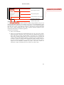
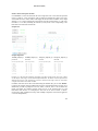
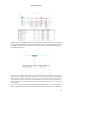
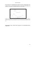
REX manual (04/09)
REX MANUAL
INTRODUCTION
While exploring experimental questions based on prior anatomical hypotheses, it is often useful
to restrict the application of statistical models to specific brain regions. In service of this goal,
SPM provides a wide range of methods for exporting image data values from image volumes at
various stages of processing or statistical modeling. The rex tool is designed to extend those
capabilities to permit the efficient extraction of image values and time series from single voxels,
voxel clusters and cluster collections. In addition to data extraction the rex tool performs ROIbased analyses of functional data complementing SPM voxel-based analyses.
While rex is part of the larger BIT toolbox, it is a single MATLAB file that may be installed and
used separately. It provides capabilities to extract image data from either a single image file or
multiple volumes such as a times-series of images. The extraction volume can be either a single
ROI or a collection of spatially disjoint ROIs. rex allows broad flexibility in the form of the
extracted data, as it can return the values of a single voxel, a single cluster of voxels or a disjoint
set of clusters. Various options are provided to generate descriptive statistics from clusters of
voxels including mean, median, voxel-weighted mean, and one or more eigenvariates. To allow
examination of experimental effects in units of percent signal change, the resulting extracted
values can be scaled with respect to either the global brain mean, or the cluster time-series mean.
rex can be accessed as a MATLAB command-line function or through a graphical user interface.
Extracted data can be saved as text and matlab data files or visualized with several data analysis
and plotting options that allow convenient data exploration and hypothesis testing.
INSTALLATION
1) If it does not already exist, create a directory named rex.
2) Copy the rex.m file (and optionally the additional TD.* files) into the rex directory
3) Start MATLAB
4) To add the rex directory to the MATLAB search path, from the File menu at the top of
the MATLAB window go to File->Set Path->Add Folder and then select the rex
directory.
5) Click Save and then Close.
The rex program is now at the beginning of the MATLAB search path.
STEP BY STEP instructions using the rex GUI
To start the ROI extraction process, at the MATLAB prompt type:
>> rex
The rex GUI should now appear on the screen.
1/9
REX manual (04/09)
Selects source volumes
Mark Pearrow 5/13/09 9:48 PM
Formatted: Font:11 pt, Font color: Black
Selects regions of interest
Data extraction options
Extracts data from source volumes
Data analyses and display
STEP 1. Selecting ROIs for extraction
Additional analysis plots
rex assumes prior creation of the regions of interest as NIFTI-1 image mask files (*.img or *.nii
formats) or text files (*.tal format). For example, if the goal is to use anatomical ROIs to guide
the functional data extraction process, you can use wfu_pickatlas to create anatomically-defined
ROIs that can be saved as *.img mask files. Note that rex permits the use of labels within mask
files in order to define multiple ROIs with a single *.img file). Alternative methods to create
functionally-defined ROIs are outlined in Appendix I.
To select one or more ROIs:
1) In the rex GUI click ROIs
2) Select one or more ROI files. The supported file types are *.nii, *.img, and *.tal files.
When using NIFTI-1 image files (.nii or .img), ROIs will be defined by the location of
those voxels where the value of the ROI image is greater than zero. In addition ROI
NIFTI-1 files containing multiple labels can also be used (the REX tool is provided with
a sample Talairach Daemon ROI file defining 55 anatomical areas in normalized space).
In contrast, * .tal files are simply text files containing the spatial coordinates (in mm) of
the voxels comprising an ROI (the x,y,z coordinates are in columns, and each voxel is a
separate row; use normalized coordinates -e.g. MNI- if the source volumes are
normalized, or subject coordinates if the source volumes are in native space).
2/9
REX manual (04/09)
STEP 2. Selecting image data sources
To define the source image files:
1) Click Sources
2) Select one or more NIFTI image volume files to extract data from these volumes
or
2) Select one SPM.mat file to extract data from volumes specified in a SPM design, or to
repeat one SPM analysis for the selected ROIs.
Selecting a single SPM.mat file instead of the NIFTI format files is equivalent to selecting all of
the image files that have been defined as the original data in the analyses specified in the
SPM.mat file (more specifically the volumes listed in the SPM.xY structure). Any valid SPM.mat
file can be used as a source, including ones resulting from either first-level or second-level
analyses. For example, if you select the first-level analysis SPM.mat file for a given subject, the
data sources will be assumed to be all of the functional data files for this subject, with one volume
for each time point across all sessions included in the SPM.mat file. In this case rex will
effectively extract all of the functional time series at the specified ROIs for this subject and allow
you to perform first-level analyses on the resulting time-series. If you select instead a secondlevel analysis SPM.mat file, the data sources will be assumed to be the beta (or con) images
specified in this analysis (one volume per regressor per subject; e.g. one contrast volume per
subject for a standard second-level t-test analysis). In this case rex will effectively extract the
beta/contrast values at the specified ROIs for each subject, and allow you to perform second-level
analyses on the resulting data.
3/9
REX manual (04/09)
STEP 3. Specify additional output options
By default rex will extract the average value within each ROI, without scaling, and without any
additional masking. Additional options include:
a) Data-level options (ROI/cluster/voxel):
Each ROI file selected in step 1 characterizes a complete region of interest (ROI). Each
ROI can be in turn formed by one or multiple clusters (disjoint sets of voxels), for
example when using a wfu_pickatlas-ROI containing multiple labels, or when using a
functionally-defined ROI composed of several clusters of activation. Last, each cluster
can be formed by one or multiple voxels. Rex allows you to extact data separately for
each voxel (voxel-level data), to extract data collapsed separately across all voxels within
each cluster (cluster-level data), or to extract data collapsed across all of the voxels
within the entire ROI (ROI-level data).
a. Use “extract data from each ROI” to extract data separately from each ROI
using the selected summary measure. The default measure is the mean, collapsed
across multiple voxels. A single output text file will be created for each ROI and
it will contain the ROI-level data for each source file in rows.
b. Using “extract data from selected clusters” is similar to extracting data from
each ROI, but if the ROI mask contains a disconnected set multiple clusters rex
will allow the user to specify a subset of clusters and the ROI-level summary
measure will only include voxels within the selected clusters.
c. Use “extract data from each cluster” to extract data separately from each
cluster within each ROI. A separate output file will be created for each cluster
and each ROI, containing the cluster-level data for each source file (rows).
d. Use “extract data from each voxel” to extract the data separately from each
voxel. A separate output text file will be created for each ROI containing the
voxel-level data across all source files (rows) and voxels (columns). In this case
the summary measure is disregarded and there is no collapsing across multiple
voxels.
b) Summary measure (mean/median/weighted mean/eigenvariates)
Note: Summary measures only apply to ROI- or cluster-level extraction
a. Use “mean” or “median” to obtain the mean or median of the data across the
selected voxels
b. Use “weighted mean” to obtain a voxel-weighted mean across the selected
voxels (not available when ROIs are defined using *.tal files). The values of the
ROI mask file at each voxel will be taken as the weights to be used when
computing a weighted average across all selected voxels. The mask values are
normalized to sum to 1 and a weighted sum is computed.
c. Use “eigenvariate” with a chosen number of eigenvariates to summarize the data
across voxels in terms of a singular value decomposition of the time series. When
choosing multiple eigenvariates the output text file (for each ROI/cluster) will
contain each eigenvariable as a column (and source files as rows as usual).
Eigenvariates are extracted using a Singular Value Decomposition (SVD) of the
time series across all the voxels within each ROI/cluster. Each eigenvariate can
4/9
REX manual (04/09)
be interpreted as a separate weighted mean of the data, where the voxel weights
are chosen to sequentially capture the maximum signal variance. For example,
the first eigenvariate represents the weighted mean of the ROI data that results in
the time series with maximum possible variance (any other weighted mean will
result in a combined signal with smaller variance). Multiple eigenvariate
extraction is useful as a data-reduction technique for multivariate analyses of
ROI data, characterizing the time series within an ROI in terms of a small
number of components that best capture the variability of responses across all of
the voxels within this ROI.
c) Scaling options (global scaling / within-ROI scaling / none)
If extracting time-series data (e.g. you chose a first-level SPM.mat file as source)
typically you would want to scale the original data within-sessions to increase the
interpretability of the data (units in percent signal change)
a. Use “global scaling” to scale the output data based on the global intracerebral
mean (SPM session-specific grand-mean scaling) of the data averaged across all
source files (or within-sessions, when a SPM.mat file is selected as source). Use
this option, for example, if you wish to extract a time-series of functional data in
units of percent signal change referenced to the SPM default intracerebral mean
of 100.
b. Use “within-ROI scaling” to scale the output data based on the local mean
(within-ROI) of the data averaged across all source files (or within-sessions,
when a SPM.mat file selected as source). Use this option if you wish to extract
time-series functional data in units of percent signal change referenced to the
mean value of each ROI)
d) Conjunction mask. Optionally you can define an additional NIFTI format conjunction
mask file. Data will only be extracted from voxels contained in this global conjunction
mask. For example, the Mask.img file generated in SPM after estimating a model can be
used to restrict all ROI data extraction to voxels within the analysis mask.
5/9
REX manual (04/09)
STEP 4. Extract and explore the data
Click “Extract” to extract the data from the source image files at the voxels inside the specified
regions of interest. A text message-box will be displayed containing the paths to the newly
created data files and a results window will display the extracted data. In addition to the output
data files (*.rex.txt files) containing the extracted data (one file per ROI/cluster), rex will create
mask files (*.rex.tal files) indicating the locations (in mm) of the voxels corresponding to the
ROI/cluster associated with each data file.
Sample GUI:
Sample output files:
TD.Middle_Temporal_G
yrus.rex.txt
TD.Middle_Temporal_Gy
rus.rex.tal
TD.Superior_Temporal_Gyr
us.rex.txt
TD.Superior_Temporal_Gy
rus.rex.tal
(one row per source file)
(one row per voxel)
(one row per source file)
(one row per voxel)
0.0630
0.0080
-0.0220
0.0326
0.0145
-0.0135
0.0114
-0.0034
-0.0641
…
-36
-34
-32
32
34
36
38
-36
-34
…
0.0548
0.0191
0.0407
-0.0092
0.0391
0.0002
0.0382
0.0603
-0.0499
…
-34
-32
-30
-28
-26
-24
26
28
30
…
2
2
2
2
2
2
2
4
4
-50
-50
-50
-50
-50
-50
-50
-50
-50
6
6
6
6
6
6
6
6
6
-50
-50
-50
-50
-50
-50
-50
-50
-50
Example of rex data extraction and display performed on second-level analysis data. The source volumes
are the subjects’ beta images, with two anatomically-defined ROIs. The effects of interest represent three
different subject groups. The extracted data (.txt files) contain the beta image values for each subject
averaged across all the voxels within each ROI.
In addition, if the data sources have been defined using the SPM.mat file, you can click “Results”
to replicate the original voxel-based SPM analyses for the extracted ROI/cluster/voxel data. As in
SPM-results you will be prompted to select (or define) a contrast, and rex will re-estimate the
model and display the statistical analysis results for all of the extracted data. For each
ROI/cluster/voxel selected rex will display the effect size for the chosen contrast, T statistic,
uncorrected p-value, and FDR-corrected p-values (multiple comparison corrections are applied to
correct for multiple ROIs).
6/9
REX manual (04/09)
Example of the rex results function used to perform SPM second-level analyses on a complete
set of anatomically defined regions (Talairach Daemon areas). Analyses are performed here on
the average activation within each ROI. Corrected p-values represent a whole-brain correction for
these ROI-based analyses.
Example of the rex results function used to perform multivariate second-level analyses on one region of
interest (Anterior Cingulate). Analyses are performed here on the first four eigenvariates characterizing the
activation profiles within the selected ROI. Corrected p-values represent a multivariate correction of each
of the individual eigenvariate results. This example illustrates the application of multivariate analyses of
ROI data showing between-group differences that would be missed if only looking at the average activation
within this ROI.
Last, if the data sources have been defined using the SPM.mat file, you can click “plots” to
further explore the effects of interest within the extracted ROIs. The options here are the same as
7/9
REX manual (04/09)
those encountered when using plots within the SPM results window, including display contrast
estimates and 90% C.I., and fitted and adjusted responses for both first-level block designs or for
second-level analyses. For event-related responses you can also explore fitted responses and
PSTHs, 90% C.Is., adjusted data, parametric responses and Volterra kernels.
Example of the rex plots function used on first-level analysis dataset in which the source volumes are
individual scans comprising a time-series extraction. The data originate from an event-related study using
famous faces (REF?) The event-related PSTH plot results for one functionally-defined ROI shown at the
right.
Please report any bugs, comments and/or suggestions to: Susan Whitfield-Gabrieli,
[email protected]
8/9
REX manual (04/09)
APPENDIX I. Functional ROI Definition
In situations where anatomical landmarks do not provide accurate guidance as to the boundaries
of regional functional specialization, so called “functional localizers” are sometimes used to
identify brain regions specialized for a particular processing function. These localizers usually
take the form of an additional task whose associated neural activity modulations are believed to
be orthogonal to the effects of interest related to the target tasks. The patterns of activity detected
by the localizer scan can then be thresholded to form a functional ROI that can be used to
spatially constrain the analysis of the target tasks. Functional ROIs may be defined in a number of
different ways:
Define a spatially localized functional ROI using the spm_VOI function
1) Copy spm_VOI.m to the spm8_first directory at the beginning of your MATLAB path.
The spm_VOI.m file replaces one that is part of the core SPM8 distribution, so it needs to
be in the MATLAB search path before the version that came with SPM8.
2) Go to SPM Results, select a contrast of interest and thresholds.
3) Choose small volume
4) Choose a Search volume using a sphere, box or image.
5)
If you have installed the modified version of spm_VOI.m, an additional figure window
will pop up with a new glass brain that has all of the voxels that survived the small
volume correction process. The descriptive statistics for these voxels are located in the
SPM graphics window. However, SPM doesn’t update the original glass brain in the
Graphics window.
6) You can now save the functional ROI in a *.tal file, an ASCII file containing the XYZ
locations of the ROI in MNI space if you are working with images that have been
spatially normalized to the MNI space..
Define a spatially localized functional ROI using xjView
1) Type >> xjview at the MATLAB command prompt
2) Navigate to the cluster of interest
3) Change the radio button from “ALL” to either “Only +” and “Only – “ (optional)
4) Choose “Pick Cluster”
5) Save the ROI mask as a NIFTI format file
Define a map-wise functional ROI in SPM
1) Go to SPM Results, select a contrast of interest and associated mask and thresholds.
2) Choose “save” to save an ROI NIFTI format file that includes all the significant voxels
in the thresholded contrast.
9/9