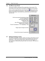
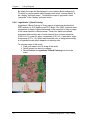
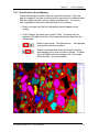
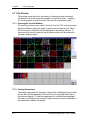
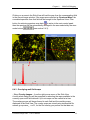
1
GENESIS MAPS/LINE – USER’S MANUAL TABLE OF CONTENTS 1 QUICK START ..............................................................................................1 1.1 Quick Start for Maps ......................................................................................... 1 1.2 Quick Start Linescan......................................................................................... 2 2 THE MAPS/LINE TAB LAYOUT ...................................................................3 2.1 The Pulldown Menu ........................................................................................... 3 2.2 The Toolbar.......................................................................................................... 3 2.3 Panel View............................................................................................................ 4 2.4 The Imaging Panel ............................................................................................. 4 2.5 The Status Bar .................................................................................................... 5 2.6 The Microscope Panel ...................................................................................... 6 2.7 Setting the Display Colors............................................................................... 6 3 IMAGING .......................................................................................................9 3.1 Collecting an Electron Image.......................................................................... 9 3.1.1 Matrix.............................................................................................................. 9 3.1.2 Reads............................................................................................................... 9 3.2 Image Processing .............................................................................................. 9 3.2.1 Auto LUT........................................................................................................ 9 3.2.2 Zooming the Image ......................................................................................... 9 3.2.3 Measurements ......................................................................................... 10 3.2.4 Annotation .............................................................................................. 10 ......................................................................................... 10 3.3 Saving an Image 3.3.1 Image Groups................................................................................................ 10 3.4 Recalling Images ........................................................................................ 10 3.4.1 Opening an Image group............................................................................... 10 3.5 Printing Images .......................................................................................... 10 3.5.1 4 and 16 View ............................................................................................... 11 3.5.2 Spectrum View.............................................................................................. 11 GENESIS Maps/Line – User’s Manual i Chapter 1 Quick Start 3.5.3 3.6 Print Setup..................................................................................................... 11 Page Setup......................................................................................................... 11 3.7 The Imaging Panel ........................................................................................... 12 3.7.1 Image Label .................................................................................................. 12 3.7.2 LUT, Save and Print ..................................................................................... 12 3.8 Image Processing ............................................................................................ 13 3.8.1 Threshold ...................................................................................................... 13 3.8.2 Spinning Mode.............................................................................................. 13 3.8.3 Multipoint Mode ........................................................................................... 13 3.8.4 Scale.............................................................................................................. 13 3.8.5 Undo.............................................................................................................. 13 3.8.6 Saving Changes............................................................................................. 13 4 SPECTRAL ANALYSIS ..............................................................................15 4.1 Collecting A Spectrum.................................................................................... 15 4.1.1 Collection Setup............................................................................................ 15 4.1.2 Preset Collection ........................................................................................... 15 4.1.3 Collection Buttons ........................................................................................ 15 4.2 Peak Identification ........................................................................................... 16 4.2.1 Auto Peak ID................................................................................................. 16 4.2.2 Manual Peak ID ............................................................................................ 16 4.2.3 HPD............................................................................................................... 16 4.3 Quantification.................................................................................................... 17 4.3.1 Standardless Quantitative Analysis............................................................... 17 4.3.2 Displaying the Quantitative Results.............................................................. 17 4.3.3 Print the Spectrum, Image and Quant Results .............................................. 17 4.4 Saving and Recalling Spectra ...................................................................... 17 4.4.1 Saving a Spectrum File ................................................................................. 17 4.4.2 Saving a Spectrum File and Associated Image File...................................... 17 4.4.3 Recalling Spectrum Files .............................................................................. 18 4.4.4 Recalling a Spectrum and Associated Image................................................ 18 4.4.5 Importing Files from other Genesis Tabs ..................................................... 18 5 X-RAY MAPPING........................................................................................19 5.1 Setup for Mapping ........................................................................................... 19 5.1.1 Location and Magnification setup ................................................................ 19 5.1.2 Dead Time and Count Rate........................................................................... 19 5.1.3 Map Type ...................................................................................................... 19 5.1.4 Map Matrix ................................................................................................... 20 ii GENESIS Maps/Line - User’s Manual 5.1.5 5.1.6 5.1.7 5.1.8 Dwell............................................................................................................. 21 Time Estimate ............................................................................................... 21 HV Off When Done ...................................................................................... 21 TTL (WDS Signal) ....................................................................................... 22 5.2 Regions of Interest .......................................................................................... 22 5.2.1 ROI’s From Peak List ................................................................................... 22 5.2.2 Auto ROI’s.................................................................................................... 22 5.2.3 Deleting an ROI ............................................................................................ 23 5.2.4 Editing an Existing ROI................................................................................ 23 5.2.5 Manually Creating an ROI............................................................................ 23 5.3 Collecting a Map............................................................................................... 23 5.3.1 Starting a Map............................................................................................... 23 5.3.2 Selecting a Name and Location for Maps..................................................... 23 5.3.3 Map Confirmation Box ................................................................................. 24 5.3.4 Map Status .................................................................................................... 24 5.3.5 Map Rescaling .............................................................................................. 24 5.3.6 Stopping a Map Before Completion ............................................................. 24 5.3.7 Auto Map Saving .......................................................................................... 25 5.4 Live Spectrum Maps........................................................................................ 26 5.4.1 Setting parameters for Live Spectrum mapping ........................................... 26 5.4.2 Collecting Live Spectrum mapping .............................................................. 27 5.4.3 Retrieving Live Spectrum data ..................................................................... 27 5.4.4 Building Maps from Live Spectrum data...................................................... 28 5.4.5 Phase Cluster Analysis of Live Spectrum data ............................................. 31 5.4.6 Building Line Scans from Live Spectrum data............................................. 33 5.5 Collecting Maps/Line with Drift Correction............................................... 34 5.5.1 Setting the Drift Correction parameters........................................................ 34 5.6 Reviewing Collected Maps ............................................................................ 35 5.6.1 Opening an Image Group.............................................................................. 35 5.6.2 The Map IPR and Text Files......................................................................... 35 5.6.3 Creating Map Overlays ................................................................................. 36 5.6.4 Map Colors.................................................................................................... 37 5.6.5 Palette Options .............................................................................................. 37 5.6.6 Logarithmic 3_Band Coloring ...................................................................... 38 5.6.7 Data Review in Quant Mapping ................................................................... 39 5.7 File Preview ....................................................................................................... 40 5.7.1 Opening the Preview Window ...................................................................... 40 5.7.2 Viewing Parameters ...................................................................................... 40 5.7.3 Gallery Files.................................................................................................. 41 5.7.4 Creating Gallery Files from Multiple Folders .............................................. 41 5.7.5 Sending Files into 16 View........................................................................... 41 Chapter 1 Quick Start 5.7.6 6. Exiting the Preview Window ........................................................................ 41 MULTIFIELD MAPPING..............................................................................43 6.1 Multifield Stage Setup..................................................................................... 43 6.1.1 Multifield Panel ............................................................................................ 43 6.1.2 Stage Control ................................................................................................ 43 6.1.3 Field Step Size .............................................................................................. 43 6.2 Setting the Stage Locations.......................................................................... 44 6.2.1 Spot Locations .............................................................................................. 44 6.2.2 Line of Fields ................................................................................................ 44 6.2.3 Matrix of Fields............................................................................................. 45 6.2.4 The Stage Table ............................................................................................ 46 6.3 Collecting and Saving MultiField Maps...................................................... 46 6.3.1 Starting Multifield Mapping ......................................................................... 46 6.3.2 Data Output Structure for Multifield Maps .................................................. 47 6.4 Reviewing Multifield Maps............................................................................. 48 6.4.1 Stub View...................................................................................................... 48 6.4.2 Loading multifield data................................................................................. 48 6.4.3 Overlaying multi field maps ......................................................................... 49 6.4.4 Manipulating Stub View layout .................................................................... 50 7.LINESCAN ......................................................................................................51 7.1 Collection Parameters .................................................................................... 51 7.1.1 Peak List........................................................................................................ 51 7.1.2 ROI’s............................................................................................................. 51 7.1.3 Count Rate, Amp Time and Dead Time ....................................................... 51 7.1.4 Collect an Electron Image............................................................................. 51 7.2 Linescan Setup ................................................................................................. 51 7.2.1 Selecting the Line ......................................................................................... 51 7.2.2 Linescan Type............................................................................................... 52 7.2.3 Number of Points .......................................................................................... 52 7.2.4 Dwell............................................................................................................. 52 7.2.5 Data Type...................................................................................................... 52 7.2.6 Time Estimate ............................................................................................... 52 7.3 Collecting the Linescan.................................................................................. 52 7.3.1 Start the Linescan.......................................................................................... 52 7.3.2 File Name and Location................................................................................ 53 7.3.3 Confirmation Box ......................................................................................... 53 Collection Status ........................................................................................................... 53 Smin and Smax ............................................................................................................. 53 iv GENESIS Maps/Line - User’s Manual 7.4 Reviewing the Linescan Data ....................................................................... 53 7.4.1 Overlaying line scan data on the image ........................................................ 54 7.4.2 Printing line scan data and the image ........................................................... 54 7.5 Plotting the Linescan Data in Microsoft Excel ......................................... 54 7.5.1 Creating the Graph........................................................................................ 54 7.5.2 Linescan Image ............................................................................................. 55 7.5.3 Printing.......................................................................................................... 55 7.5.4 Saving ........................................................................................................... 55 8 MICROSCOPE CONTROL..........................................................................57 8.1 Setting and Reading the Microscope Parameters .................................. 57 8.2 kV On and Off.................................................................................................... 57 8.3 Auto CPS ............................................................................................................ 57 8.4 Auto Functions ................................................................................................. 57 8.5 Stage Control .................................................................................................... 57 8.5.1 Stage Movement ........................................................................................... 57 8.5.2 Stage Coordinates ......................................................................................... 58 8.6 Auto Update....................................................................................................... 58 Chapter 1 Quick Start vi GENESIS Maps/Line - User’s Manual Chapter 1 1 QUICK START 1.1 Quick Start for Maps Quick Start 1. Set a preset for spectrum collection. 2. Select an appropriate amp time to obtain a dead time between 20 and 40 percent. 3. Collect an image. 4. Collect a Spectrum 5. Identify the peaks. 6. Select the Map type. 7. Select a Matrix size, Dwell and the Data Type. 8. Start the map. A dialogue box will open to select a file name and location to save the maps. GENESIS Maps/Line - User’s Manual 1 Chapter 1 Quick Start 1.2 Quick Start Linescan 1. Set a preset for spectrum collection. 2. Select an appropriate amp time to obtain a dead time between 20 and 40 percent. 3. Collect an electron image. 4. Collect a spectrum. 5. Identify the peaks. 6. Switch to Linescan. 7. Click on the draw line button. Click and drag the mouse on the image to draw the line. 8. Select the number of points, a dwell for collection at each point, the data type and if desired, check the Quant box for a Quant linescan. (A time estimate based on the number of points and the dwell will be displayed in the status bar at the bottom of the screen.) 9. Begin the linescan. A dialogue box will open to select a file name and location. 10. When finished, Microsoft excel will open automatically with the collected data displayed. Plot the linescan using the chart wizard. 2 GENESIS Maps/Line - User’s Manual Chapter 2 2 Maps/Line Layout THE MAPS/LINE TAB LAYOUT The layout of the Map/ Line tab is similar to that of the both the Spectrum and the Imaging tab. The majority of the screen in the analysis area with a control panel on the right hand side of the screen and a pull down menu and button bar across the top 2.1 The Pulldown Menu The pull down menus across the top of the screen provide access to advanced features as well as different screen views. 2.2 The Toolbar The Tool bar in the Maps/ Line Panel displays fast buttons for processes that are frequently used. Open a file Import a spectrum from other Genesis tabs Save a File Print Annotate Image/ Map Zoom, Measure on Map or Image Screen View (single image, four images, 16/36 images, image and spectrum, 8/18 images and spectrum) Multi field Stub View Enable external scan Raster mode (Full scan, reduced area, spot, hand drawn) Send data to Microsoft Word Template Select EDS Detector Set preset acquisition time, Select the time constant Main Maps/ Line panel, Microscope control. GENESIS Maps/Line - User’s Manual 3 Chapter 2 2.3 Maps/ Line Layout Panel View Most of the major functions that will be utilized in the Maps/ line panel the majority of the time can be accessed in the main Maps/ line panel. This panel is the default panel view on the right hand side of the screen. If any of the advanced panels are accessed, the main panel can be returned to by clicking on the panel button on the right hand side of the button bar. Collect an Electron Image Collect or clear a spectrum Auto Peak Id/ Conformation Select a map or a linescan Map type Start an X-Ray Map Use Z List to automatically define ROI’s Turn of the kV when maps are completed Auto Look up Table Modification Print Multifield Mapping 2.4 The Imaging Panel The second panel that is available in the Maps/ Line tab is the Imaging panel. The imaging panel allows for the collection of images, selection of imaging parameters and some image processing. The imaging panel can be accessed from the “Set Up” pull down menu. 4 GENESIS Maps/Line - User’s Manual Chapter 2 Maps/Line Layout Edit boxes for the kV and magnification Collect an electron image. Continuous image collection Image label, detector number, minimum and maximum signal range to be mapped to 0-255 gray scale, and the number of reads (integration factor) Autoscale (Find the video signal range) Auto Look up table for contrast adjustments Save the current file Print an image or multiple images Adjust the contrast and brightness of the imagerelative to the image on the microscope. Tilt Correction 2.5 The Status Bar The Status bar appears at the bottom of the screen and displays pertinent information for imaging, spectrum collection, mapping and linescans. From left to right the status bar shows: Counts per second, the dead time, Collection time in live seconds, number of counts in the channel under the cursor, the location of the cursor, the full scale value of a displayed spectrum, the memory needed for the current map or linescan set up and an estimated time for the map or linescan collection. GENESIS Maps/Line - User’s Manual 5 Chapter 2 2.6 Maps/ Line Layout The Microscope Panel This panel can also be accessed if the system has column control. The microscope control panel can be accessed by clicking on the microscope button on the far right hand side of the button bar. See section 8 for more on the microscope control panel. The parameters displayed may be different depending on what features are authorized by the microscope manufacturer. Set the microscope Accelerating voltage Set the magnification Set the working distance Change Spot Size Turn HT on/ off Auto CPS function/ View Geometry Stage Control Features: Current Coordinates: X, Y, Z, R(roatate), T (tilt) Stage map and stage movement Auto poll microscope for parameters 2.7 Setting the Display Colors The colors of the panels, spectrum, buttons and many other features can be changed in the Set Colors window that can be accessed in the “View” pull down menu. Using the drop down menu, select one of the features. A color can then be selected by using the either color choices, RGB values or the palette. 6 GENESIS Maps/Line - User’s Manual Chapter 2 GENESIS Maps/Line - User’s Manual Maps/Line Layout 7 Chapter 3 3 Imaging IMAGING Many of the imaging features from the Image tab are available in the Maps/ Line panel. Digital images can be collected from the microscope and processed using annotation, measurement and modification of the look up table. 3.1 Collecting an Electron Image Collecting an Electron image can be accomplished by clicking on the “Collect Image” button in the main Maps/ Line panel. 3.1.1 Matrix The image matrix size can be selected by right mouse clicking on the text to the right of the image collection button. 3.1.2 Reads Type the desired number of reads into the edit box. The reads are the number of times that data will be sampled at each pixel and then averaged together. From one to 9999. 3.2 Image Processing Many of the basic image processing tools found in the Image tab are available in the maps/ line tab as well. 3.2.1 Auto LUT The LUT (look up table) button modifies the look up table so that the first time the button is clicked the table adjusts so that the image histogram is stretched to represent the full greyscale value. The second time the button is clicked the brightest and darkest 1% are excluded and the histogram is stretched to portray the image with a higher contrast. The third click restores the look up table to the original values. 3.2.2 Zooming the Image An image can be zoomed by clicking on the magnify button in the button bar. Click and drag a box with the mouse over the area of interest. The zoom can then be pasted in an open window by selecting “Zoom to clipboard” in the “Edit” pull down menu, clicking on an open window in 4 or 16 view, and paste (“edit” pull down) the zoom in the window. The zoom can then be saved by clicking on the zoom window and hitting the save button. (See section 5.1 of the Image manual.) GENESIS Maps/Line - User’s Manual 9 Chapter 3 Imaging 3.2.3 Measurements Measurements can be made on a map or image by enabling the measurement button in the button bar. Draw a line on the feature to be measured. The measurement (in microns) will appear in the status bar at the bottom of the screen. (See section 5.2 of the Image manual.) 3.2.4 Annotation The image can be annotated with text, location markers, measurements and collection conditions. To annotate the image, click on the ‘T’ button in the tool bar or select “Annotate” from the edit pull down menu. The annotation window will open and display options for annotation. To burn a crosshair or a rectangle on the image be sure that the collection mode is set in the desired method. (See Section 5.4 of the imaging manual) 3.3 Saving an Image Once an image has been collected it can be saved as either a bitmap (.bmp) or a tiff (.tif) file. To save the image click on the “Save” button on the bottom of the main imaging panel or select “Save As” from the “file” pull down menu. Browse for the desired location, select a name and file type (.bmp or .tif) and then hit enter. 3.3.1 Image Groups To save a group of images that are related use a common root name, Sample1 for example, and then a different extension for each of the separate images. (Sample1_lowmag, Sample1_himag, for instance). These images are now considered to be an image group and can be recalled together. (See section 3.4.1) 3.4 Recalling Images Images can be recalled by selecting “Open” from the “File” pull down menu or hitting the “Open” button in the button bar. Browse for the desired file, highlight it in the list and click “Open”. 3.4.1 Opening an Image group A group of related images saved with the same root name can be opened as a group. (For example sample11_loc1, sample11_loc2). To open a group of images select the file type Image group (.bmp or .tif) and then highlight one of the files in the list that has the root name. All of the images will open into the sixteen-view screen mode. 3.5 Printing Images Printing Images can be done in single, four, sixteen and spectrum view. Use the print button at the bottom of the main Maps/ Line panel, the print 10 GENESIS Maps/Line - User’s Manual Chapter 3 Imaging button in the button bar, or select “print” from the file pull down menu. The selected printer and the page orientation are displayed to the right of the printer button. 3.5.1 4 ,16 and and 36 View In four, sixteen, and 36 view mode only the images that are highlighted (hold down the ctrl key and click on the image or images) will be printed. 3.5.2 Spectrum View In spectrum view the image will be printed in the upper left hand portion of the page with the spectrum in the lower portion and either the image parameters or the quant results in the upper right hand side. 3.5.3 Print Setup To select a different printer or access the printer properties window, right mouse click on the text to the right of the Print button for access to Printer set up dialogue box. 3.6 Page Setup Under the “File” pull down menu, the selection for “Page Set” allows for the selection of printing options. If printing both an image and a spectrum, both must be selected in this window. Other options, such as the kV and the magnification can be printed under the image if desired. GENESIS Maps/Line - User’s Manual 11 Chapter 3 3.7 Imaging The Imaging Panel The Imaging panel can be accessed in the Maps’ line panel by selecting “Image” in the “Set Up” pull down menu. This allows for the features available in the Image tab to be accessed in the Maps tab as well. 3.7.1 Image Label The image parameters, including matrix, reads and strips can be set and a label can be given to the image. 3.7.2 LUT, Save and Print The Auto LUT table button can be used and the image can be saved and printed. 12 GENESIS Maps/Line - User’s Manual Chapter 3 3.8 Imaging Image Processing The Image processing panel can also be accessed in the Maps/ line tab. Image Processing includes three methods of Image rescaling. To access the rescale panel, select “Rescale” from the “Process” pull down menu. 3.8.1 Threshold The first button is the Threshold mode where the cursors can be moved to isolate a portion of the histogram that is to represent the entire range of the histogram. 3.8.2 Spinning Mode The second mode that is available is the spinning mode which has a fixed point and modifies the levels around this point. 3.8.3 Multipoint Mode The Multipoint button mode allows the user to adjust the histogram in a nonlinear mode. 3.8.4 Scale Pressing scale button sets the adjustments that were made to the image. 3.8.5 Undo The undo button offers one level of undo. 3.8.6 Saving Changes The image is not saved with the changes automatically so closing and reopening the image will restore the image to its original greyscale levels if the changes have not been saved. GENESIS Maps/Line - User’s Manual 13 Chapter 4 4 Spectral Analysis SPECTRAL ANALYSIS The Maps/ Line tab offers many of the spectrum analysis features that are available in the spectrum tab. Collection, peak identification and standardless quantification are available with the added benefit of having the image displayed on the same screen as well. The screen view must be set so that image is shown in the upper left hand window, the image histogram in the upper right and the spectrum shown below. To switch to this mode select the screen mode button (in the main button bar) that shows the screen divided into three sections. 4.1 Collecting A Spectrum Spectra can be collected and the peaks identified as is done in the Spectrum tab. 4.1.1 Collection Setup As with spectra collection in the Spectrum tab, correct set up is necessary for accurate quantitative and qualitative analysis. The correct time constant, based on the counts per second, should typically be selected to obtain a dead time between twenty and forty percent. The amp time is selected from the drop down box in the button bar. 4.1.2 Preset Collection A preset for spectrum collection time can also be set by selecting or editing the desired collection length in the Preset drop down box. No preset Clock Time Live Time (add a L to preset) 4.1.3 Collection Buttons The buttons that are used for collection include buttons in the main mapping panel for collection and peak identification as well as buttons located above the spectrum collection window for collecting and viewing the spectrum. GENESIS Maps/Line - User’s Manual 15 Chapter 4 Spectral Analysis 4.2 Peak Identification Peak Identification can be performed as in the spectrum tab. There are buttons in the main panel for auto ID as well as HPD. The panel can be expanded for manual peak identification or adjusting the auto id list. 4.2.1 Auto Peak ID Auto ID can be performed at any time during or after spectrum collection. It is appropriate to use the auto peak identification when 1. All peaks are well defined 2. There are no difficult peak overlaps 3. The spectrum has been collected for an adequate amount of time. To perform an auto identification of the peaks, click on the Peak ID button in the main maps/ line panel. 4.2.2 Manual Peak ID When manual identification is necessary, the peak identification portion of the window can be expanded so that the manual id features are available. There are two main methods of manual identification. ¾ In the Element edit box type either the element name or the elements number and hit enter to display the element markers. To add the element in the list click the “Add” button. ¾ Click on the peak of interest. Scroll through the Possible element list to find a probable match. Highlight the element to be added to the peak ID list and click “Add”. ¾ The Z- and Z+ buttons are available whenever an element is displayed in the element list box. The buttons allow the user to easily select additional elements that are of a similar atomic number by stepping through the periodic table starting with the element in the element list box. 4.2.3 HPD The HPD (Halographic peak deconvolution) uses the spectrum collection parameters and the element list to draw a theoretical spectrum to compare with the collected spectrum. The HPD appears as an outline drawn over the collected spectrum. If the HPD is misfit for a particular element, that peak can be reexamined. To view the HPD click on the HPD button in the main maps/line panel. To remove the HPD right mouse click anywhere in the spectrum area 16 GENESIS Maps/Line - User’s Manual Chapter 4 4.3 Spectral Analysis Quantification Spectra collected in the maps/ line software can be quantified using the standardless quantification routine. 4.3.1 Standardless Quantitative Analysis To perform a standardless quantification press the Q button found in the button bar above the spectrum collection window. You can select the background subtraction method and the SEC factors as set up in Spectrum Tab, from the dropped down menu of Q button. 4.3.2 Displaying the Quantitative Results The results, as atomic and weight percents, will be displayed in the upper right hand portion of the analysis window where the image histogram is usually displayed. The results can be removed by clicking on the X in the top right hand corner of the Q results window. 4.3.3 Print the Spectrum, Image and Quant Results To print the quantification, press the print button while the Quant results are viewed on screen. The results will be printed with the spectrum and image displayed as well. 4.4 Saving and Recalling Spectra Spectra can be saved and recalled as done in the spectrum and imaging tabs. 4.4.1 Saving a Spectrum File To save a spectrum file click on the save button in the button bar or “Save As” in the file menu can be used. Select .spc as the file type. (In the maps panel, the default file type will be .bmp.) Select a file location and name and then click save. 4.4.2 Saving a Spectrum File and Associated Image File A Spectrum and a corresponding image can be saved with the same file name by selecting “image and spectrum” from the file pull down menu. This will save two separate files, one .spc and one .bmp, with the same name. Note that the image will not include the red marker for the beam location during the collection of the spectrum. It is possible to add the location using the annotate image function in section 3.2.4. GENESIS Maps/Line - User’s Manual 17 Chapter 4 Spectral Analysis 4.4.3 Recalling Spectrum Files Spectrum files can be recalled by clicking on the file open button in the button bar or by selecting “open” from the file pull down menu. Switch to .spc as the file type, browse for and select the desired file and then click open. The “File or Current Parameters” window will open. In this window, the user has the option to open the file with the element list, regions of interest, background and analysis conditions saved with the file, or, with the settings that are currently in use. A combination of both saved and current settings can be used. Select the desired parameters and then click “Ok”. Use the “all current” or “all file” for easy selection if not using a combination of both. The “View” button display a window with the stored set up and collection parameters. 4.4.4 Recalling a Spectrum and Associated Image If the spectrum was saved along with a corresponding image the files can also be opened simultaneously by selecting “spectrum and image” as the file type. The confirmation boxes for both the image and the spectrum file will appear. 4.4.5 Importing Files from other Genesis Tabs Spectra files can be imported from other Genesis tabs by clicking on the Import Spectrum button in the main toolbar or by selecting “Import Spc from” from the file pull down menu. Select ‘Restore’ to bring back the previous spectrum. 18 GENESIS Maps/Line - User’s Manual Chapter 5 5 X-Ray Mapping X-RAY Mapping The maps/ line tab allows the user to select different x-ray map types, collect up to 15 elemental maps simultaneously and create maps overlays. Maps are saved as image files and can be recalled and processed. 5.1 Setup for Mapping Setting up for mapping involves not only the set up parameters but the collection parameters as well. Before mapping, be sure that the area of interest is displayed on the microscope, is in focus and at the correct working distance. 5.1.1 Location and Magnification setup Set the microscope to the correct location and magnification. Select an accelerating voltage that is appropriate for the element list of the sample. As with spectral analysis, the rule for selecting an accelerating voltage is that the beam energy should be at least two times the energy of the highest energy peak in the spectrum. Remember that the magnification of the map is also important as the higher the magnification the smaller the pixel size. Make sure that the beam diameter or the interaction volume is not significantly larger then the features on the map. 5.1.2 Dead Time and Count Rate In mapping, throughput is very important as the dwell per each pixel is very short. Select a count rate for high throughput but without causing the sample to charge or drift. Select a time constant that will give a dead time of between 20 and 40 percent based on the count rate being used. The time constant (amp time) is selected using the drop down box found on the right hand side of the button bar. 5.1.3 Map Type Several types of maps are offered in the EDAX Maps/ Line tab. Standard maps are included on every system with the Maps/ Line tab. Live Spectrum maps and Quant maps are options available in the maps/ line panel. If the options are available, select the map type by checking either: ¾ “live” or ¾ “live” and “spc” ¾ or “quant” or ¾ check neither for a standard map. GENESIS Maps/Line - User’s Manual 19 Chapter 5 X_Ray Mapping ¾ Standard maps collect x-ray data at every pixel for the selected dwell. The data for that pixel is then recorded and the map updated. ¾ Quant mapping collects data in the same way as standard mapping. However, at every pixel a complete background subtraction and peak deconvolution is performed. The data type for a Quant map may include Net Intensities, k-ratio and ZAF. Note: In a Quant map with ZAF weight percent as the data type, only one line for a given element can be used in the quantitative routine, and therefore mapped. If more than one line is identified, one will be removed from the ROI list. For example, if Iron K and L are in the peak ID list, only Iron K will be mapped. If the user would like to include multiple lines for an element, they should select “Net” maps as the data type. ¾ Live Mapping rasters very quickly over the entire map area and presents the data for the entire map (1 frame). This is repeated and the maps are updated until the map is stopped by the user or when the set number of frames is reached. This technique is also called fast mapping. ¾ Live Spectrum Mapping rasters frame after frame over the entire map area storing the entire spectral information, while updating the images and the cumulated spectrum. This technique is the most efficient way of collecting data at high speed. After collection you can retrieve the entire spectrum at a selected location in the image or you can build compositional maps of any available type, including Quant maps. 5.1.4 Map Matrix The map matrix should be selected based upon the magnification, size of the samples features and the desired time of collection. Maps can be collected at resolutions between 64x50 and 2048x1600. To select the matrix size right mouse click to the right of the Maps collect button. Select the desired matrix size from the list. The text to the right of the Maps collect button will now update to show the selected matrix size. 20 GENESIS Maps/Line - User’s Manual Chapter 5 X-Ray Mapping ¾ For fine-featured samples, a smaller matrix size (64x50) may not be appropriate as the pixel will be larger than the feature. ¾ At high magnifications, a larger matrix size can result in the pixel size being smaller than the diameter of the beam or the interaction volume. ¾ The larger the matrix size, the longer the collection time. If a long dwell is being used, the map will take slightly longer, but the matrix size will increase the length of collection time more significantly. 5.1.5 Dwell The dwell is the amount of time that the beam will collect at each pixel. The dwell for both standard and quant maps is in milliseconds. For live maps the dwell is in microseconds. Select a dwell based on the count rate and the concentrations of the elements of interest. The dwell must be long enough to gather enough counts that the data is statistically accurate. The lower the count rate and the concentration of the elements the longer the dwell must be. ¾ For Live maps, the dwell will default to be two times the processing time. The dwell can be lengthened but cannot be shortened. ¾ For Quant maps a minimum dwell of 50 milliseconds is required. Since a background subtraction and peak deconvolution is completed at each point, the dwell must be longer for this to be accomplished accurately. ¾ For Live Spectrum maps a minimum dwell of 50 microseconds is required. A minimum dwell of 200us is recommended for 128x100 matrix, 100us for 256x200 and higher. ***Note: When a Quant map is begun, a dialogue box may appear prompting the user to increase the count rate or to lengthen the dwell. If this is not practical, the map can be started by clicking OK. To cancel and lengthen the dwell or increase the count rate, click on cancel. Adjust the desired parameters and then start the map again. 5.1.6 Time Estimate For standard, quant and spectrum maps a time estimate for the map will be displayed in the bottom status bar and will update as the parameters (matrix and dwell) are adjusted. For live and live spectrum maps no time estimate is given, as the maps can be stopped at any time. 5.1.7 HV Off When Done For long, unattended collection, the system can be set so that the microscope beam can be turned off once collection has finished. This GENESIS Maps/Line - User’s Manual 21 Chapter 5 X_Ray Mapping feature is available on some systems with column control. To enable this feature, check the “HV off when done” box in the main Maps/ Line panel. 5.1.8 TTL (WDS Signal) The WDS mapping option adds an external TTL input source, to the list of ADC and EDS acquisition types. This allows for other types of data to be acquired simultaneously, such as a WDS map. To enable this option check the TTL checkbox located between the options for Live and Quant Mapping. 5.2 Regions of Interest Regions of Interest (ROI) are created to define the energy range from which counts will counted for a particular element. The region of interest list is created automatically from the peak ID list and it can be edited or manually created. 5.2.1 ROI’s From Peak List If no ROIs are created by the user, auto regions of interest can be created from the peak ID list when the map is started. To have the ROI list created automatically, check the “Use peak list” check box in the main Maps/ Line panel. 5.2.2 Auto ROI’s The ROI’s can also be set by selecting “ROI’s” from the “Set Up” pull down menu and click on the “Auto ROIs” button. Auto creation of the regions of interest will create an ROI for each element in the peak ID list. If two lines of the same element are identified in the peak ID list (FeK and FeL, for example) two regions of interest will be created and therefore, two maps will be collected for that element. If a quant map, with the data type ZAF weight percent, is collected, one of the lines will automatically dropped when the map is started, as two lines for the same element cannot be used in the quantification routine. If an element is not to be mapped for, it can be removed from the peak ID list and it will not mapped. If the element needs to be labeled in the spectrum, but the map is not to be collected, the ROI list can be edited. (See section 5.2.3) 22 GENESIS Maps/Line - User’s Manual Chapter 5 X-Ray Mapping 5.2.3 Deleting an ROI From the ROI panel an element can be removed from the list, a created region adjusted or one or more regions of interest can be created manually. To delete an ROI, highlight the element to be removed and click the delete button. All of the ROI’s can be deleted by clicking on “Delete All”. 5.2.4 Editing an Existing ROI To alter an existing ROI, highlight the ROI in the list, change the start and/ or end keV in the Edit boxes and then hit “Change”. The values in the list and the ROI drawn on the spectrum will both be updated. 5.2.5 Manually Creating an ROI To create an ROI, click on the create button. The cursor will now turn to an arrow. Click and drag on the spectrum where the new ROI is to be created. The start and end values will be diplayed in the Edit boxes. The start and end values can also be typed directly into the edit boxes if that is preferred. Type in a name (3 characters) and then click “Add”. The created ROI will now be added to the list. 5.3 Collecting a Map Once the parameters and sample have been set for analysis the map can be started. The map will be collected for the current field. 5.3.1 Starting a Map To start the map, click on the “Collect Maps” button in the main Maps/ Line panel. Before the map is begun, two windows will be displayed for naming the maps, confirming the map parameters and giving the map a title. 5.3.2 Selecting a Name and Location for Maps The first window that will appear is for selecting a location and file name for the maps. The file name that is given will be the root name that is used for every map. The name will then automatically be given an extension of the element symbol and the line for each map. (Sample11_FeK, Sample11_NiK, for example) Type the name and then click on “Save” to continue. Long file names can be used but certain special characters, such as a period or an underscore, should not be used because the software will add an underscore to designate the image group. GENESIS Maps/Line - User’s Manual 23 Chapter 5 X_Ray Mapping 5.3.3 Map Confirmation Box The second window that appears will list the parameters of the map including a time estimate and a comments box. This comments box is used to create a title for the maps and will be displayed at the top of the page when the maps are printed. When the parameters have been checked and a title entered, click “OK” and the map will begin. If no title is desired, leave the box empty and click “OK”. 5.3.4 Map Status While the map is collecting, the time estimate will update in the status bar. The CPS will be displayed in red while collecting and when finished will switch to black. If the mapping panel is expanded, the full range of values (Smin and Smax) will be displayed for each element. The data displayed is for the data type selected for the map. 5.3.5 Map Rescaling The maps will automatically rescale to reflect the full value range as the map is collected. 5.3.6 Stopping a Map Before Completion To stop a map before the map is completed, click on the “Collect maps” button again. It may take a few seconds before the map is actually stopped. Standard and Quant maps will not be saved if they are stopped 24 GENESIS Maps/Line - User’s Manual Chapter 5 X-Ray Mapping prior to completion. If live maps are stopped before completing the preset number of frames there will be a dialog box asking if the maps are to be saved, stopped immediately or at the end of the current frame. 5.3.7 Auto Map Saving Once the map is completed, the map files will be saved automatically with the root file name selected before the map collection and the element extension. GENESIS Maps/Line - User’s Manual 25 Chapter 5 5.4 X_Ray Mapping Live Spectrum Maps Live spectrum maps have additional setup parameters for collection and enhanced processing and review features. 5.4.1 Setting parameters for Live Spectrum mapping Select Live and Spc options from Genesis Maps control panel. Select Spectrum Mapping options from the right mouse menu in the control panel. - Select the elemental peaks in the Peak Id panel and validate them in the Z List dialog. Buttons used for reviewing and processing Spectrum maps. - Select the dwell time per pixel (minimum 50 microseconds). - Select the number of frames from right mouse menu. 26 GENESIS Maps/Line - User’s Manual Chapter 5 X-Ray Mapping 5.4.2 Collecting Live Spectrum mapping Press Collect X Maps button to start. A pop up window will prompt you to select the output folder and root file name. During collection the following items will be updated every couple of seconds: The cumulative spectrum will be updated in the Spectrum View. The maps for the selected elements in the Z list. The status bar will update the total counts aquired in the cumulative spectrum(TotC:), the time to collect a frame (FT:ussualy ~3 sec for 128x100 resolution, 12 sec. for 256x200,…) , the number of line data waiting in the queue to be processed (Queue:) and the number of frames. If the processing queue is building up, select a longer dwell time per point. The collected data will be saved in following files: A BMP ( or TIF ) file with video image. A SPC file with total cumulated spectrum and parameters. A SPD file with individual spectrum data for every pixel in the image. You can stop the collection before the selected number of frames have been completed, by clicking the Collect button, with the option to save the data. 5.4.3 Retrieving Live Spectrum data Select Spectrum map data file type (SPD) in the File Open dialog. Selecting a SPD file, the application will load the video image (BMP) stored under the same name and the cumulated spectrum (SPC). GENESIS Maps/Line - User’s Manual 27 Chapter 5 X_Ray Mapping To inspect the spectrum at individual locations selected in the image: Select Data from the Display menu or clicking button in the main control panel. Select Hand drawn from the toolbar icon , click and draw on the image to review the average spectrum from the selected area. Select Spot scan mode from the toolbar icon specific location in the image. Select Reduced scan mode form the toolbar icon spectrum in the selected area. to review the spectrum at a to accumulate the Note: When in Spot or Reduced mode use the directional keys + SHIFT key down to scroll through entire image: the spectrum view will be updated on the fly with corresponding data. You can also accumulate the spectrum from the image areas of a selected gray level. - Select areas in the image using the threshold bar in the image histogram and press the Color Area button to visualize the selection. - Click Build Spc button to accumulate the spectrum from the selected area. 5.4.4 Building Maps from Live Spectrum data - Select Spectrum map data file type (SPD) in the File Open dialog, as in paragraph 5.4.3 above. - Select the elemental peaks in the Peak Id panel and validate them in the Z List dialog. 28 GENESIS Maps/Line - User’s Manual Chapter 5 X-Ray Mapping - Click the Build Spc Maps button in the main control panel to start maps building. - A dialog will prompt you to select the data type for maps. - Select the data type for the maps (ROIs, Net Intensities, K-Ratios or ZAF-wt%) and click OK. - Select the output folder and file name. GENESIS Maps/Line - User’s Manual 29 Chapter 5 30 X_Ray Mapping GENESIS Maps/Line - User’s Manual Chapter 5 X-Ray Mapping 5.4.5 Phase Cluster Analysis of Live Spectrum data - A new method of statistical analysis of spectral mapping data is offered, allowing the user to automatically find phases in the recorded data, by clustering spectra at each pixel based on similarity in the channels counts. No prior knowledge of elements, sample type or microscope conditions is required. Load a spectrum map file (.SPD) and click Phase Analysis button in Xmaps Panel: A new control panel will pop up, allowing the user to: - Build automatically or manually the phase clusters - Build phase maps based on selected clusters. - Find the best phase matches for a spectrum from any area of the image. - The phase clusters can be manually edited by adding/deleting/replacing or labeling the phases. Up to 16 phases can be added to the library in this version. - The right mouse menu of this panel allows for saving/retrieving the clusters in/from a phase library (.PCL). Find Clusters: Automatically find phases in the recorded data, by clustering spectra at each pixel based on similarity in the channels counts (using Chi-Square fit contingency coefficient). Pixel Avg: For improved statistic spectra used in the match are cumulated/averaged from an area of selectable size. Fit(%): Fit threshold used in the ChiSquare fit. Auto Fit: Fit threshold is determined dynamically in several data scan iterations if the check box is checked, otherwise the value edited by user is used. Use BSE: The BSE video data can be selected as an additional channel in the analysis. GENESIS Maps/Line - User’s Manual 31 Chapter 5 X_Ray Mapping Reviewing the phases: - Clicking an item in the phase list will bring the corresponding spectrum in the background of the spectrum view. - Clicking + ALT key will bring the corresponding spectrum in the foreground of the spectrum view, so that the Peak Id funcions could be used and the phase could be properly labeled. - Clicking + CTRL key will add the new selected phase to the background overlay of the spectrum view. Build Map: - Phase Maps can be built using the phase library, associating a color to each pixel in the image based on the closest found phase in the library and the goodness of fit. In the phase list select the phases to be used in the map, with CTRL key pressed. For this version select maximum of seven phases, so that the available color palette of maps overlay can be used. It is a good practice to delete first the phases with a count of one in the list, then selecting the phases with the highest number of counts. The phase legend shown in the histogram view is available for printing. If Use BSE is selected, the average electron image signal is shown in the status bar. 32 GENESIS Maps/Line - User’s Manual Chapter 5 X-Ray Mapping Match Spc: - The phase library can be used to match the current foreground spectrum and give a list with the fit numbers for the closest matched phases. 5.4.6 Building Line Scans from Live Spectrum data - Select Spectrum map data file type (SPD) in the File Open dialog, as in paragraph 5.4.4 above. - Select the elemental peaks in the Peak Id panel and validate them in the Z List dialog as in paragraph 5.4.4 above. Select the Line radio button. - Select the line scan width from the right mouse menu of the control panel. The data at each point will be integrated from a number of map pixels (1, 3x3, 5x5,…) around the line point. - Select a line on the image using - Click button, as described in section 7.2.1. button to start building the line scan from stored spectrum maps data. GENESIS Maps/Line - User’s Manual 33 Chapter 5 5.5 X_Ray Mapping Collecting Maps/Line with Drift Correction The Drift Correction option can be used to compensate for the drift in the image while collecting maps or line scans in specific conditions (high magnification or stage drift). The Drift correction works with any of maps type or line scans. - Select 'Drift' check box in Maps/Line Panel. An image will be collected automatically from the central area of the field of view (it will appear as it if had been collected at a higher Mag). At the same time the Edax Drift Shell will be launched minimized in the task bar. - Start maps collection by clicking the 'Collect X Maps' button. The drift correction sequence (collecting image, correlating with reference image, applying drift correction to the beam control) will automatically be initiated at the selected drift rate (minimum 10 sec recommended), completely transparent to the application. You can bring up the drift shell from time to time just to see the drift map, if interested. A log .CSV file is generated during collection and saved in the same folder with your data. It contains information on all the drift points, so it can be reviewed in Microsoft Excel. 5.5.1 Setting the Drift Correction parameters The EDAX Drift Shell comes with appropriate default setting so that it can be used right away. The shell can be used also outside any application to monitor and log the microscope image drift for a period of time. Right mouse click on the Drift Shell icon if launched in the task bar and select 'Restore' to bring it up on your screen. You can leave the shell minimized during maps collection (it comes with appropriate default setting), or Select 'Drift'-Settings' menu, just to check following settings : In the first tab of the dialog: - Drift Correction Rate (15 sec default) - Max drift count (4000 default) : how many drift points will be logged in the drift map. - Drift method : always use 2 in this version. In the second tab of the dialog select the reference image settings: - Matrix (256x200 default) - Integration factor (100 default) - Full Scan Percentage (50% default): the remaining percentage of the scan range is used to track the drift. 34 GENESIS Maps/Line - User’s Manual Chapter 5 5.6 X-Ray Mapping Reviewing Collected Maps The maps will be displayed in the sixteen-view mode while collecting and when they are completed. The maps can also be opened from file at a later date and reviewed. 5.6.1 Opening an Image Group Opening an Image group is the best way to open an entire set of maps. The maps are all saved as individual files with the same root name and the element and line as an extension. To open the entire set of maps select “Image Group” (either bmp or tif) as the file type and then highlight one of the maps from the group and click “Open”. All of the maps with that Root name will be opened into the sixteen-view mode. 5.6.2 The Map IPR and Text Files With each map additional files are saved which record the image parameters (an .ipr file and a .txt file). To view the information from the ipr file select “Image parameters” from the edit pull down menu. The Image Parameters file for a map contains the collection conditions such as matrix size, kV, magnification, data range, dwell, time constant, take off angle and data type collected. The signal will be the element and the line associated with the map. The pixel size and field size are also displayed. The comments field can be used for any notes that are pertinent to the sample. The text file can be viewed with any text viewing program. When copying files to another drive or location copy the two image parameters files as well as the image file. GENESIS Maps/Line - User’s Manual 35 Chapter 5 X_Ray Mapping 5.6.3 Creating Map Overlays Creating an overlay of up to six maps can be completed in the sixteen-view screen view. To create an overlay, highlight each of the maps to be in the overlay by holding the control key and clicking on the desired maps. With the maps highlighted select “Color”; “substitution overlay” from the “Process” pull down menu. There must be one open window in which the overlay can be viewed. The overlay will be displayed in the first open window. It will automatically be saved with the root name of the maps and the extension ovXX. The XX will be the number of the window in which the map was created. In the example below, the map would be saved with the extension _ov11. Note: The overlay is created by selecting the element with the brightest normalized pixel intensity to represent that pixel in the overlay. It may be best select a single element that represents a phase rather than selecting all the elements. 36 GENESIS Maps/Line - User’s Manual Chapter 5 X-Ray Mapping 5.6.4 Map Colors The color of the map can be changed after collection if desired. To do this, highlight the map to be changed and select “Image parameters” from the edit pull down menu. Select a color from the drop down list in the color box. Click “Ok” to close the window. The map color will change on the screen. To save the color change, highlight the map and click on save. If the maps are reopened the color will be the new color. 5.6.5 Palette Options Following color palettes are selectable from the Display Menu: Displaying the maps in different palettes enables the maps to be displayed and printed on either a black background, white background or in greyscale. GENESIS Maps/Line - User’s Manual 37 Chapter 5 X_Ray Mapping By default the maps will be displayed in color palette (black background). To switch to reverse palette (white background) select “reverse palette” in the “display” pull down menu. To display the maps in greyscale, select “greyscale” in the “display” pull down menu. 5.6.6 Logarithmic 3_Band Coloring Logarithmic 3-Band Coloring of X-ray maps is a technique developed at NIST Institute, by D.E. Newbury and D.S. Bright, Dec.1998. It permits direct comparison of maps of different elements in the same field of view or maps of the same element in different areas. Three color bands are defined, associated with intensity ratio of each element: blue for trace intensities (0.001 to 0.01), green for minor components (0.01 to 0.1) and red for major components (0.1 to 1.0). Within each band the color is assigned according to a logarithmic scale which depends on intensity ratio. To compare maps in this mode: ¾ Load your maps in the 16-Image View mode. ¾ Select images you want to compare. ¾ Select Process > Logarithmic 3-Band Coloring from the main menu. 38 GENESIS Maps/Line - User’s Manual Chapter 5 X-Ray Mapping 5.6.7 Data Review in Quant Mapping In quantitative maps the data (value) is saved for each pixel. When the map is completed, the data can be viewed for each pixel or a selected area. Data for multiple elements can be viewed simultaneously. To view the data, highlight the maps from which the data is to be viewed. ¾ Switch to single view (the first highlighted map will appear on the screen). ¾ In the “Display” pull down menu, select “Data”. A column will now appear on the right hand side of the image showing the data from the entire image. Switch to spot mode. The data will now for the pixel under the crosshair. be displayed Switch to selected area mode and draw (by clicking and dragging) a box over an area of interest. The data will now update to be the average of all of the pixels within the area. (As shown below) GENESIS Maps/Line - User’s Manual 39 Chapter 5 X_Ray Mapping 5.7 File Preview File preview mode allows for the viewing of thumbnails and comments/ conditions for all of the maps and images in a particular folder. A gallery file, an association of files of interest, can also be created and saved. 5.7.1 Opening the Preview Window To open the preview mode, select “Preview” from the “File” pull down menu. Select the folder in which the maps to preview are located and hit “Open”. All of the maps in that folder will be displayed in the preview window. If there are more then 40 maps the up and down buttons will be enabled to view the remaining maps. 5.7.2 Viewing Parameters The image parameters for the map or image that is highlighted (surrounded by blue box) will be displayed in the text box on the top right hand side of the preview window. To view the parameters for a different map highlight the map by clicking the mouse on the map of interest and the information in the parameters window will update. 40 GENESIS Maps/Line - User’s Manual Chapter 5 X-Ray Mapping 5.7.3 Gallery Files A gallery file, a collection of up to 16 maps and images of interest, can be created containing any of the maps in the preview window. Select one of the maps of interest. Right mouse click on the map and drag the map into the lower 16 windows. Repeat this for any other maps of interest. When all of the maps have been brought into the lower windows click on the “Save” button at the bottom of the screen. From the “Save As” window select a name and location for the file. The file type will default to gallery file (.glr). The gallery file can be read back into the preview window at a later time by clicking on the “Read” button at the bottom of the preview window. 5.7.4 Creating Gallery Files from Multiple Folders Gallery files can be created from maps in different folders as well. Open the preview window as described above and select the files from the first folder to be added to the gallery. Click on the directory button in the preview window button. Browse for the folder that contains the next maps to be added to the gallery. Open the new folder and add the maps to the gallery. Repeat until all the desired maps have been added. 5.7.5 Sending Files into 16 View The selected maps in the lower window can be brought into the 16-view mode to be viewed, printed and/ or processed. To do this, click on the 16view button at the bottom of the preview screen. All of the images in the lower windows will be brought into the 16-view in the maps/ line tab. A gallery file can also be opened and then brought into 16-view in the same way. 5.7.6 Exiting the Preview Window To exit the preview mode, click “OK”. GENESIS Maps/Line - User’s Manual 41 Chapter 6 6. Multifield Mapping MULTIFIELD MAPPING Multi-field mapping allow the user to collect maps from multiple fields unattended. Multifield mapping is possible on systems with stage and column control. This is available if the user has stage control software on their EDAX system. For multi-field mapping the set up begins the same way as set up for a single field analysis. Remember that the time estimate for the maps is for a single map. The multi-field run will be this time multiplied by the number of maps that will be collected. For live maps there should be a set number of frames for the maps to work within the available time as multi-field maps. 6.1 Multifield Stage Setup In the multifield set up panel, accessed by expanding the multifield portion of the main mapping panel, the stage can be moved to the desired locations using the EDAX stage control if desired. 6.1.1 Multifield Panel To select the stage locations, the multi-field panel should be accessed by expanding the multi-field mapping area at the bottom of the main mapping panel. 6.1.2 Stage Control The stage control at the top of the panel can be used to move the stage during set up. The arrows on the stage diagram will move the stage in that direction, one field taking the current magnification into account. If the x and y coordinates are known, they can be typed directly into the edit boxes below the stage diagram. 6.1.3 Field Step Size The field step size is the number of fields that the stage will be moved when the blue arrows on the stage diagram are clicked. This number can be changed so that field is moved less than or more than one field at a time. GENESIS Maps/Line - User’s Manual 43 Chapter 6 6.2 Multifield Mapping Setting the Stage Locations Setting the stage locations begins by selecting the arrangement of the multiple fields. Fields can be individual locations, multiple fields along a line or a matrix of fields covering both the x and y direction. 6.2.1 Spot Locations Random spot locations can be set at particular areas of the sample. Select “Point” as the type. The set up window will display a button labeled “First” above X and Y coordinate boxes. ¾ Set the microscope to the first location to be mapped. Click on the “First” button. The X and Y coordinates will up date to the current stage location. ¾ Click on the “Add” button to save this as a field. The field will now appear as position one. ¾ Move the stage to the second location to map. Click on the “First” button to read the coordinates and then “Add” to enter the field as position two. ¾ Repeat this for all of the locations to be mapped. A 44 6.2.2 Line of Fields line of map fields can be created by selecting a first and last point along a line. Select “Line”. The window will update to have “first” and “last” boxes with x and y coordinate boxes for each. ¾ Position the stage at the beginning of the line. Click the “First” button. The coordinates for the first map will be displayed below. GENESIS Maps/Line - User’s Manual Chapter 6 Multifield Mapping ¾ Move to the position of the last map to be collected. Click on the “Last” button. The coordinates for the last map will now be displayed below. ¾ If a particular number of maps are to be collected across the line the adjacent fields box can be left unchecked and the field divided by the number of maps either overlapping or leaving gaps between the maps. ¾ Click on “Add Line” too determine the fields and add them to the list, If the maps are to be collected as neighboring fields, check the “Adjacent field” box. For adjacent maps, the line can be determined using a set number of points, and the magnification changed so that there are adjacent fields across the line or the current magnification can be used and the number of fields determined based on that magnification. Select the desired choice below the adjacent fields check box. ¾ When the fields are added a dialogue box will appear displaying the magnification to use or the number of fields and the percentage of the area covered. The fields will be added to the box below the x and y coordinate boxes. 6.2.3 Matrix of Fields A matrix of fields can also be created similar to the creation of a line but in both the x and the y direction. ¾ Position the stage at the top corner of the matrix. Click the “First” button. The coordinates for the first map will be displayed below. ¾ Move to the position of the last map to be collected, the opposite, lower corner. Click on the “Last” button. The coordinates for the last map will now be displayed below. ¾ If a particular number of fields are to be collected from the given area, the adjacent fields box can be left unchecked and the fields will be best fit GENESIS Maps/Line - User’s Manual 45 Chapter 6 Multifield Mapping into the area between the first and last points. Click on “Add matrix” to add the determined fields to the list. ¾ Select adjacent fields to create a matrix of neighboring fields. The matrix of fields can also be determined using either a given number of points, or the current magnification. If a specific number of points are to be used, select number of points and type in the number of fields in both the x and y direction. When the matrix is added a dialogue box will display the magnification to use. The current magnification can also be used and the number of points determined so that best fit that magnification. Once the selection has been made click on “Add Matrix” to add the fields to the list 6.2.4 The Stage Table The created stage table will be saved automatically when the multifield run is started. It will be saved as an .stg file in the main folder. 6.3 Collecting and Saving MultiField Maps Collecting and saving x-ray maps from multiple fields is similar to collection and saving for a single field. Select an appropriate kV, magnification, matrix, dwell and count rate as described in the set up sections for mapping (5.1 and 5.2). 6.3.1 Starting Multifield Mapping - Click on the “Multifield” button at the bottom of the panel. This will bring up a dialogue box for creating/selecting the root folder where the multifield data set will be stored. 46 GENESIS Maps/Line - User’s Manual Chapter 6 Multifield Mapping - Create a new folder by clicking Make New Folder button. When the folder has been created/selected, click OK. - You will be prompted to select a Group file name. Here you can edit the File name and click Save. After reporting a summary of the collection settings the multifield run will start. During the analysis the status (moving stage, collecting maps) will be displayed at the bottom of the panel. 6.3.2 Data Output Structure for Multifield Maps Assuming the folder created in the first dialog was Multifield6 and the group name selected in the second dialog was edaxmaps.bmp, the maps will be stored in the following folder structure: In each field folder the field number is appended to the filename as well as the identifier for the element (_AlK,…) or electron image label (_Img). GENESIS Maps/Line - User’s Manual 47 Chapter 6 6.4 Multifield Mapping Reviewing Multifield Maps 6.4.1 Stub View Click on the Stub View button in the main toolbar. This will bring up a view for selecting/reviewing the data from a multi field run. Right mouse clicking anywhere in the Stub View will bring up a menu for selecting and reviewing the data from a multifield run. 6.4.2 Loading multifield data - Select Open… from the right mouse menu of the Stub View. - In the File Open dialog box select one .BMP image file from any field of the multifield data set. This will load all the corresponding images/maps from all related fields. The Stub View will show initially the fields layout. - Select Show Images from the right mouse menu of the Stub View. The images/maps selected will be shown in the corresponding location of the Stub View. 48 GENESIS Maps/Line - User’s Manual Chapter 6 Multifield Mapping Clicking on an area in the Stub View will load the map from the corresponding field in the current Image window. If the maps were collected as ‘Spectrum Maps’ the cumulated spectrum from that field will be brought in the Spectrum View. If the button for retrieving spectrum map data is active in the main control panel, then the spectrum will be automatically averaged in the area selected by the scan mode buttons (see section 5.4.3). 6.4.3 Overlaying multi field maps - Select Overlay Images… from the right mouse menu of the Stub View. A multi select dialog box will be prompted for selecting the maps available in the currently open multi field data set. Up to six maps can be overlaid at a time. The overlay process will be performed in each field and the resulting maps displayed in the Stub View. The overlay maps are stored using incremental file names: group name_ + ov01, for the first overlay you perform on that data set, GENESIS Maps/Line - User’s Manual 49 Chapter 6 Multifield Mapping group name_ + ov02, for the second time, etc. You can recall previously stored overlay maps via right mouse Open… menu. 6.4.4 Manipulating Stub View layout You can adjust the fields layout in the Stub View as following: - Click on the Stub View title bar to get keyboard focus. Use SHIFT+ directional keyboard keys to adjust the space between fields in horizontal and vertical directions. - Select Invert X/Y Axis Orientation from the right mouse menu of the Stub View to reverse the order of fields displayed in either direction. This might be necessary to accommodate differences in stage movements and beam scanning directions of various microscopes. - Select Full View from the right mouse menu of the Stub View to show the stub in full view. 50 GENESIS Maps/Line - User’s Manual Chapter 7 Linescan 7.LINESCAN Linescans collect data at a series of points along a line and plot the data as a graph. Lines can be drawn across the area of interest horizontally, vertically or diagonally. 7.1 Collection Parameters Setting up a linescan is similar to the starting of a map. The element list and the collection parameters must be optimized for the desired time and sample characteristics. 7.1.1 Peak List Collect a spectrum from the whole area as well as scanning in spot mode on various phases to establish a representative peak identification list. 7.1.2 ROI’s Select the method of ROI creation. Check “Use Peak list” in the main panel, or create ROI’s as described in section 5.2. 7.1.3 Count Rate, Amp Time and Dead Time Select a count rate that will allow for an adequate through put in a short dwell but will not charge the sample or cause the sample to drift. Based on the selected count rate, chose an amp time that will give a dead time of 20 to 40 percent. 7.1.4 Collect an Electron Image Collect an image (“Collect e-” button) of the area that is to be used for the linescan. The matrix size of the image used during a linescan will not affect the collection time of the linescan. 7.2 Linescan Setup Click on the Line button in the Main Maps/ Line panel. The map section will now be updated so that the collection parameters will be applicable to the linescan. 7.2.1 Selecting the Line Click on the button. The image will be transferred into single view and the cursor will be come an arrow. Click and drag the mouse over the image where the linescan is to be collected. If the line is to be redrawn or was drawn incorrectly, click the “Draw Line” button again and redraw the line on the image. GENESIS Maps/Line - User’s Manual 51 Chapter 7 Linescan 7.2.2 Linescan Type Select between a standard linescan or a quant linescan. In a standard linescan, a spectrum will be collected at each point and the number of counts within the region of interest will be recorded in the linescan. Be sure that the Quant box is unchecked below the “Line” button. In a quant linescan, the data will be collected as it is in a standard linescan but a background subtraction and peak deconvolution will be performed at every pixel. To select a Quant Linescan, check the Quant check box below the line button. 7.2.3 Number of Points In the “Points” edit box, type the number of locations to be collected along the line. 7.2.4 Dwell A dwell (collection length) per point must then be entered (in milliseconds) in the “Dwell” edit box. A longer dwell (minimum of 50msec) will be required for a quant linescan in order to generate enough counts within a peak to perform the background subtraction and peak deconvolution. 7.2.5 Data Type Right mouse click below the dwell edit box to select the type of data that is to be collected. For a standard map the only data type will be available is ROI counts. For a Quant linescan, select the desired data type from the list. The choices are: ROI counts- number of counts within the region of interest Net Intensities- Number of counts in a region of interest after a background subtraction and peak deconvolution. K-ratios- Ratio between the measured and theoretical pure values ZAF Wt- weight percents calculated with the Z, A and F corrections 7.2.6 Time Estimate When the number of points and the dwell have been entered, a time estimate will be displayed in the bottom status bar. 7.3 Collecting the Linescan When all of the linescan parameters have been set the linescan can be started. The data will collect for each point and be saved to a .csv (comma separated values) file. 7.3.1 Start the Linescan Click on the “Collect Line” button to start the linescan. 52 GENESIS Maps/Line - User’s Manual Chapter 7 Linescan 7.3.2 File Name and Location Select a location and file name for the linescan in the displayed window. The file type must be .csv. The image, with the line, will be saved as a bitmap file with the same name automatically. 7.3.3 Confirmation Box A confirmation box will be displayed with the collection parameters and the time estimate. Click “OK” to begin the linescan. Collection Status A red cursor will display at the current collection location on the line during the collection. When the collection is finished, Microsoft Excel will be opened automatically. Smin and Smax If the linescan panel is expanded while collecting the minimum and maximum values (Smin and Smax) can be viewed for each element. The data type is ROI counts for a standard linescan or the selected type for a Quant linescan. 7.4 Reviewing the Linescan Data You can review the Linescan data in Microsoft XL or using the LscanDsp utility. To review the Linescan data using the LscanDsp click button in the Line panel. The LscnDsp utility will open showing the data collected in the last Linescan run. To review an older data set open the corresponding .CSV file from File > Open menu in the LineScan utility window. GENESIS Maps/Line - User’s Manual 53 Chapter 7 Linescan 7.4.1 Overlaying line scan data on the image To display both the image and the line scan data, select Show Image from the Image menu and Horizontal from ImgOvly menu. 7.4.2 Printing line scan data and the image To print the line scan data and the image, select Print from the File menu in the Line Scan utility window. 7.5 Plotting the Linescan Data in Microsoft Excel Plotting the linescan in Microsoft Excel will create a graph showing elemental distribution across the line. 7.5.1 Creating the Graph The linescan can be plotted using either the number of points or the distance across the line (in microns) as the X-axis the results as the Y-axis. Select the data to be plotted by highlighting the desired cells. 54 GENESIS Maps/Line - User’s Manual Chapter 7 Linescan Use the Chart Wizard to plot the graph (using the XY scatter plot option works well). The graph can be customized to show only certain elements, change the line color or the point style by right mouse clicking on the portion of the graph to be changed. (Use the Microsoft Excel help files for more detailed instructions) 7.5.2 Linescan Image The image that is saved with the linescan has the same name that was given to the linescan and saved as a bitmap. By right mouse clicking in the plot area a dialogue box for the plot area can be displayed. Using the “Fill Effects” in the plot area dialogue, this picture can be added to the background of the linescan. 7.5.3 Printing To print the linescan, use the print button in the button bar of Microsoft excel. The graphic can also be copied and pasted into a report. 7.5.4 Saving The linescan is automatically saved as a CSV file that can be read into Microsoft excel. Once the graphic has been created, it must be resaved as an .xls file format in order to save the created linescan graphic. If only the data is to be saved it does not have to be resaved. GENESIS Maps/Line - User’s Manual 55 Chapter 8 8 Microscope Control Microscope Control On systems with Column control, the microscope control panel can be accessed by clicking on the Microscope panel button on the right hand side of the button bar. This panel is customized for each microscope type and your panel might have a different appearance. 8.1 Setting and Reading the Microscope Parameters The microscope parameters, including kV, Magnification, working distance and spot size are read from the microscope. These parameters can also be changed from the EDAX software by typing the new value into the Edit box and hitting enter. The microscope parameters will then be updated. 8.2 kV On and Off The beam can be shut off or turned on by clicking on the HT button on microscopes that support this feature. 8.3 Auto CPS The CPS button allows the user to select a target count rate and have the spot size adjusted accordingly. When the CPS button is hit, an edit box will appear to the right of it. Type in the desired count rate and press the enter key. While the system is adjusting, the CPS will be in red. When the adjustment is finished, the CPS will be displayed in black. 8.4 Auto Functions The auto buttons in the Microscope control panel are for Auto focus course and fine, Auto stigmate and auto brightness and contrast. 8.5 Stage Control The stage control portion at the bottom of the screen can be used to move the stage to a desired location. The stage movements are limited to the stage movements that are motorized on the microscope. 8.5.1 Stage Movement The stage can be moved in 1-field increments by clicking on any of the directional arrows. To move the stage in increments that are greater or less than one field, type the desired number of frames in the center of the octapad. GENESIS Maps/Line - User’s Manual 57 Chapter 8 Microscope Control 8.5.2 Stage Coordinates The Parameters that are displayed are the x and y location as well as Z, tilt and rotation. Not all parameters can be read on all microscopes. 8.6 Auto Update The Auto Update check box, when enabled, has the EDAX system poll the microscope at frequent intervals for the microscope settings. The settings are also polled immediately before and image, spectrum, map or linescan is collected. 58 GENESIS Maps/Line - User’s Manual Chapter 8 GENESIS Maps/Line - User’s Manual Microscope Control 59