Download eta/VPGTM SIMULATION TRAINING MANUAL

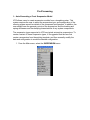
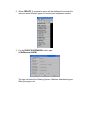
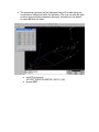
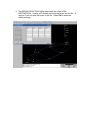
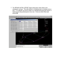
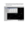
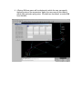
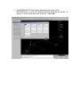
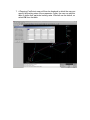
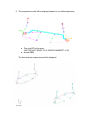
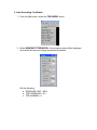
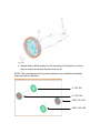
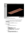
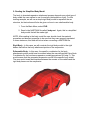
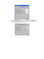
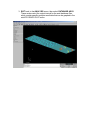
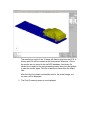
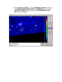
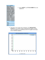
eta/VPGTM
Version: 3.0
SIMULATION
TRAINING MANUAL
Mechanical System Simulation Package
Release Date: April, 2004
FOREWORD
The concepts, methods, and examples presented in this text are for illustrative
and educational purposes only, and are not intended to be exhaustive or to apply
to any particular engineering problem or design.
This material is a compilation of data and figures from many sources.
Engineering Technology Associates, Inc. assumes no liability or responsibility to
any person or company for direct or indirect damages resulting from the use of
any information contained herein.
Engineering Technology Associates, Inc.
1133 East Maple Road, Suite 200
Troy, MI 48083
Phone:
(248) 729-3010
Support:
(800) ETA-3362
Fax:
(248) 729-3020
Engineering Technology Associates, Inc., ETA, the ETA logo, and eta/VPG are
the registered trademarks of Engineering Technology Associates, Inc. All other
trademarks or names are the property of the respective owners.
Copyright 1998-2004 Engineering Technology Associates, Inc. All rights
reserved
Table of Contents
Introduction_____________________________________________________6
eta/VPG Menu System
6
Opening/Creating an eta/VPG Database File
9
Pre-Processing_________________________________________________11
1- Auto-Generating a Front Suspension Model
11
2- Auto-Generating a Rear Suspension Model
19
3- Auto-Generating Tire Models
27
· Defining Initial Rotational Velocity
30
4- Auto-Generating a Road Surface
· Defining Contact between Road and Tires
· Constraining the Road
· Assigning Velocity to the Road
32
33
34
34
5- Reading the Simplified Body Model
· Defining Gravity
· Pre-loading the Suspension
36
38
38
Dynamic Analysis_______________________________________________40
6- Defining VPG Analysis Control Parameters
40
7- Analysis Submission
45
Post-Processing________________________________________________46
8- Displaying Results
46
9- Graph Plotting
52
Conclusion____________________________________________________54
Engineering Technology Associates, Inc.
Creation Date: December 15, 1998
Revision Level: 6
Revision Date: April 2, 2004
Approved by: T. Palmer
Introduction
Introduction
This tutorial was created to familiarize new users with the eta/Virtual Proving
Ground (VPG) software, and provide a guide on the techniques used to create
vehicle system models. The following exercises will show the user how to
generate suspensions (front/rear), tires, and road models using the eta/VPG
software. To complete the vehicle system model, a simplified vehicle body will be
added to the suspension and the full system model will be analyzed and the
results post-processed.
eta/VPG Menu System
The menu system is an open system. Most operations are accessible at any
time during the eta/VPG session. The user interface consists of four parts: the
Drawing Area, Menu Area, Dialogue Area, and Display Parameter Options Menu.
The menu system is set up as a tree structure. The program starts in the MAIN
menu and branches out into sub-menus. The user selects a sub-menu by mouse
pick or keyboard entry. Descriptions for these menu options are located in their
respective sections.
The Main Menu is located at the top of the VPG window, and provides access to
the main VPG functions. All pre-processing functions are found on the PRE
menu. In previous versions of eta/VPG the PRE menu would be found on the
Main menu when opening a database.
FILE:
PRE:
PARTS:
ROAD:
SUSPENSION:
TIRE:
SAFETY:
ANALYSIS:
FATIGUE:
POST:
GRAPH:
UTILITIES:
VIEW:
HELP:
Imports and exports data to and from VPG.
Contains a menu of pre-processing functions. All menus
such as ELEMENTS, NODES, LINE, SURFACE, MODEL
CHECKER, MATERIAL PROPERTY, ELEMENT
PROPERTY and CONTACT INTERFACE are found in this
menu.
Creates and modifies Parts.
Selection and creation of Road Surface Models. Only
available in the DYNA environment.
Creates and modifies suspension system models using a
template system. Also allows for import of ADAMS data.
Only available in the DYNA environment.
Creates Tire Models. Only available in the DYNA
environment.
Creates vehicle impact and safety simulations using a
process guidance tool. Only available in the DYNA
environment.
Set-up of analysis parameters and specification of output.
Analyzes element fatigue.
Provides options for viewing the results of an analysis.
Plots dynamic characteristics of the structure vs. time,
velocity, etc.
VPG user environment settings, including analysis solver
type, and viewing parameters.
Manipulates the display, position, and perspective of a
model.
Contextual on-line help. Accesses the eta/VPG User
Manual.
Function Keys
Function keys 1 through 8 direct the user to the most frequently used menus.
The F1 (function key 1) is reserved for the Main Menu.
F1
F2
F3
F4
Main Menu
Element Option
File
Geometry Builder
F5
F6
F7
F8
Model Checker
Node Options
Surface Options
Pre Processor
Display Window
VPG breaks the screen into five distinct regions. The regions are used to receive
input or display messages for the user. The five regions are illustrated on the
following page.
1. DRAWING WINDOW -- Models and definition cards are displayed in this
area.
2. MENU AREA -- Commands and command options are displayed in this area.
They can be accessed via the keyboard mouse.
3. DIALOGUE / PROMPT AREA -- VPG displays comments and messages to
the user and accepts keyboard entry commands in the dialogue window.
4. DISPLAY PARAMETER OPTIONS WINDOW -- These commands set the
plot options for the current model.
Menu
Area
Dialogue/Prompt
Area
Display
Parameters
Options Window
Opening/Creating an eta/VPG Database File
Type ‘vpg’ in a Unix window to start the program. Once the windows are
activated, the VPG FILE MENU window is displayed for the user to OPEN or
CREATE a new VPG database.
1. The user would either select the name of a previously saved file or
enter the name of a new file in the Dialogue window. The
recommended practice is to add the extension .vpg to a newly created
file.
2. If creating a NEW file, the user would be prompted to do so:
3. The user will be prompted to select the analysis program desired:
The analysis program selected will set defaults for the eta/VPG
session to generate LS-DYNA, NASTRAN, RADIOSS, PAM-CRASH
ABAQUS, MOLD-FLOW or GENESIS models.
To access all of the features required to perform a typical VPG
simulation, the user must select DYNA. This selection then allows the
user to access the Tire, Suspension and Road Surface menus. For the
purposes of this tutorial, the user should select DYNA.
4. The user will also be prompted to select the Unit System desired. It is
convenient for users to select the MM, TON, SEC, N unit system, since
this results in stress values that are in MPa.
The user will now be in the MAIN MENU of eta/VPG and ready to start
the session.
Pre-Processing
1- Auto-Generating a Front Suspension Model
VPG allows users to create suspension models from a template system. This
system requires the user to select the suspension type, and configuration of the
steering system as well as details of the component configuration. In addition, the
user should have the geometry points of the suspension, and the bushing and
spring stiffnesses and the damping characteristics of any system components.
The suspension types supported in VPG are typical automotive suspensions. To
create a variant of these suspension types, it is suggested that the user first
create a suspension from the existing template, and then manually modify the
data and configuration to model the desired configuration.
1. From the Main menu, select the SUSPENSION menu.
2. Select CREATE. A suspension menu will be displayed from which the
user can select different types of front and rear suspension models.
3. For the FRONT SUSPENSION, select type:
2- McPherson A-ARM
The user can select the Steering System, Stabilizer Attachment types,
Ride Spring type, etc.
4. The suspension geometry will be displayed along with a table listing the
coordinates of nodes that define the geometry. The user can edit this table
to define their particular suspension geometry. We shall use the default,
so select OK from the table.
a. eta/VPG will prompt:
‘ACCEPT THESE GEOMETRY DATA? (Y/N)’
b. Answer YES.
5. A Spring Stiffness menu will be displayed in which the user can specify
the spring rates of the suspension. Again, the user can edit this table to
define their particular spring rates. We shall use the default, so select OK
from the table.
6. The SPRING PRINT FLAG table determines the output of the
DECFORCE file. A value of 0 (default) will write the forces into the file. A
value of 1 will not write the forces to the file. Select OK to enter the
default settings.
7. The SPRING INITIAL OFFSET table determines initial offset in the
suspension springs. The initial offset is a displacement or rotation at time
zero. For example, a positive offset on a translational spring will lead to a
tensile force being developed at time zero. Enter an initial offset and
select OK.
8. A Damping Coefficient menu will then be displayed in which the user can
specify the bushing rates of the suspension. Again, the user can edit this
table to define their particular bushing rates. We shall use the default, so
select OK from the table.
9. An Extra Node Coordinate menu will then be displayed in which the user
can specify the coordinates of the body attachment points of the
suspension. Again, the user can edit this table to define their particular
body attachment points. We shall use the default, so select OK from the
table.
a. Eta/VPG will prompt:
ACCEPT EXTRA NODE COORDINATES? (Y/N)
b. Answer YES
10. The suspension model will be displayed based on our defined geometry.
a. Eta/VPG will prompt:
USE STRUCTURE MASS, CG, & INERTIA MOMENT? (Y/N)
b. Answer YES
2- Auto-Generating a Rear Suspension Model
1. Select CREATE. A suspension menu will be displayed from which the
user can select different types of front and rear suspension models.
2. For the REAR SUSPENSION, select type:
3- MCPHERSON H-ARM
The user can select the Stabilizer attachment point location.
3. The suspension geometry will be displayed along with a table listing the
coordinates of nodes that define the geometry. The user can edit this table
to define their particular suspension geometry. We shall use the default,
so select OK from the table.
4. A Spring Stiffness menu will be displayed in which the user can specify
the spring rates of the suspension. Again, the user can edit this table to
define their particular spring rates. We shall use the default, so select OK
from the table.
5. The SPRING PRINT FLAG table determines the output of the
DECFORCE file. A value of 0 (default) will write the forces into the file. A
value of 1 will not write the forces to the file. Select OK.
6. The SPRING INITIAL OFFSET table determines initial offset in the
suspension springs. The initial offset is a displacement or rotation at time
zero. For example, a positive offset on a translational spring will lead to a
tensile force being developed at time zero. Enter an initial offset and
select OK.
7. A Damping Coefficient menu will then be displayed in which the user can
specify the bushing rates of the suspension. Again, the user can edit this
table to define their particular bushing rates. We shall use the default, so
select OK from the table.
8. An Extra Node Coordinate menu will then be displayed in which the user
can specify the coordinates of the body attachment points of the
suspension. Again, the user can edit this table to define their particular
body attachment points. We shall use the default, so select OK from the
table.
9. The suspension model will be displayed based on our defined geometry.
a. Then eta/VPG will prompt:
‘USE DEFAULT MASS, CG, & INERTIA MOMENT? (Y/N)’
b. Answer YES.
The front and rear suspensions will be displayed.
3- Auto-Generating Tire Models
1. From the Main menu, select the TIRE MODEL menu.
2. Select GENERATE TIRE MODEL. A tire property menu will be displayed
from which the user can change the desired properties.
Edit the following:
a. PRESSURE UNIT = MPa
b. TIRE PRESSURE = 0.2
c. TIRE NUMBER = 4
3. The tire profile will be shown.
a. eta/VPG will prompt:
‘DO YOU ACCEPT THIS TIRE PROFILE? (Y/N/ABORT)
b. Answer YES.
c. eta/VPG will then prompt for tire location:
‘DEFINE WHEEL CENTER LOCATION FOR TIRE 1’
1. Select the SPINDLE option from the Control Keys menu.
2. Pick the node at the end of one of the 4 spindles for tire
#1.
4. Repeat step to define location for the remaining 3 tires (define in a clockwise or counter-clock-wise direction from tire #1.
NOTE: The joints between the tires and suspension are created automatically
when the tires are attached.
0, 750, 350
0, -750, 350
2500, 750, 350
2500, -750, 350
Defining Initial Rotational Velocity
1. Turn off all suspension parts (parts 1-381) leaving only the tires on.
2. Create 2 PART_SETs, the first set for the 2 front tires, the second set for
the 2 rear tires.
a. Select PRE-PROCESSOR/SET MENU/PART/CREATE
b. VPG prompts:
‘ENTER PART SET NUMBER (DEFAULT) OR E TO EXIT’Select enter.
‘PICK AN ELEMENT OR PART NAME OF A PART’
c. Use a MULTI-POINT REGION to select all of the parts of the 2
front tires.
d. Select EXIT.
3. Repeat step 2 and define a PART_SET for the 2 rear tires.
4. Create 2 Velocity cards, 1st for the front tires PSID, 2nd for the rear tires.
Select PRE-PROCESSOR/BOUNDARY CONDITIONS/INITIAL
CONDITION CARDS/VELOCITY/CREATE/GENERATION.
a. Edit the following on CARD 1:
1. CARD DESCRIPTION- user defined.
2. STYP(SETTYPE)= 1(PART SET).
3. ID(ID)- select PART SET ID corresponding to the set
number defined in STEP 2.
4. OMEGA(ANGULAR VELOCITY)= road velocity/tire
radius. In order to make the rotation velocity compatible
to the translation velocity, the tire geometry size should
be used here. The formula is:
V = VT * Rθ
R = RRIM + RTREAD
RTREAD = W * Ratio
b. Edit the following on CARD 2:
1. Xc- tire center coord for front tire Local Coord. System
measured in step 4b.
(front=0.0, rear=2500.0)
2. Yc- tire center coord for front tire Local Coord. System
measured in step 4b.
(front=0.0, rear=750.0)
3. Zc- tire center coord for front tire Local Coord. System
measured in step 4b.
(front=350.0, rear=350.0)
4. Nx=0.0
5. Ny=-1.0 (negative or positive depending on velocity sign
and Right Hand Rule of LCS).
6. Nz=0.0
5. Repeat step 4 for the rear tire PSID.
4- Auto-Generating a Road Surface
1. Select ROAD from the Main menu.
2. Choose SELECT FROM LIBRARY.
a. Select USER DEFINED.
b. VPG prompts:
ENTER USER DEFINED ROAD FILE OR “STOP” TO EXIT’
1. Type in ‘road.lib’.
2. Select 1-COBBLESTONE.
3. As you will notice, after the road model is read in, the road is located
underneath our suspension model. If the road model were not located in
the correct position, the MOVE ROAD SURFACE would be used to
position the road correctly.
NOTE: Put the model into a SIDE view. Small adjustments may have to be made
to the road location by using the PRE-PROCESSOR/NODE/TRANSFORM
command to transform the nodes of the road up or down in the global Z direction.
The goal is to have 1 to 2 mm gap between the tires and road surface (no
penetration). This distance can be checked by using the DISTANCE NODE/PT
command in the UTILITIES menu.
·Defining Contact Between Road and Tires
1. Turn off all but the outer tread part of each tire and the road surface.
2. Select PRE-PROCESSOR/CONTACT INTERFACE/CREATE/3DIMENSIONAL
3. Select 5-NODES_TO_SURFACE interface type.
4. Edit the following:
a. CARD 1
1. CARD DESCRIPTION (eg. tire 1)
b. CARD 2
1. SSID(SLAVE ID) - tire #1 PID
2. MSID(MASTER ID) - road PID
3. SSTYP(SLAVE TYPE) - ID type=4(NODE-SET)
4. MSTYP(MASTER TYPE) - ID type=2(PART)
c. CARD 3
1. FS(STATIC FRICTION COEFF.) - 0.7.
2. FD(DYNAMIC FRICTION COEFF.) - 0.7.
5. Use the COPY command to copy the 1st interface card to generate cards
for the remaining 3 tires. Edit the CARD DESCRIPTION, CID(contact
interface ID), and SSID for each respective tire.
Constraining the Road
1. Turn ONLY the Road Surface ON.
2. Select PRE-PROCESSOR/MATERIAL.
3. Select DEFINE PROPERTIES, and pick the material assigned to the road.
4. The material card appears, edit the following on CARD 2:
a. CON1= 5
b. CON2= 7
NOTE: This will constrain the road in the Y, Z and all rotational directions.
Assigning Velocity to the Road
When defining the road, the user has the option of a moving or fixed surface. If
the road is fixed, this step is not necessary and should be skipped.
1. Select PRE-PROCESSOR/BOUNDARY CONDITIONS/BOUNDARY
CARDS/PRESCRIBED MOTION/CREATE/RIGID BODY.
2. Edit the following to the BOUNDARY_PRESCRIBED_MOTION card:
a. CARD DESCRIPTION - (e.g. road vel.)
b. PID(PART ID) - select the road PID
c. DOF(Degree of Freedom) - select 1- X- TRANSLATION
d. VAD(VELOCITY,ACCEL,DISPL) = 0(velocity)
e. LCID(LOAD CURVE ID):
1. DEFINE CURVE OPTION/CREATE
2. CURVE DEFINITION CARD
No editing, select OK.
3. VPG prompts:
‘ENTER DATA(TIME & VALUE) FOR POINT 1 OR END’
Enter: 0, 16000(mm/s).
4. VPG prompts:
‘ENTER DATA(TIME & VALUE) FOR POINT 2 OR END’
Enter: 10, 16000(mm/s).
NOTE: The time value of 10 (secs) is arbitrary, we will not be running the job for
that long.
5. VPG prompts:
‘ENTER DATA(TIME & VALUE) FOR POINT 3 OR END’
Type ‘end’.
6. The load curve is displayed along with the curves menu.
7. EXIT the curves menu.
5- Reading the Simplified Body Model
The body to chassis/suspension attachment process depends upon what type of
body model the user wishes to use for analysis (deformable or rigid). For this
training example, we will use a simple rigid body model to represent the car
structure, but instructions will also be given on how to use a deformable body.
1. From the Main Menu, select FILE.
2. Read in the NASTRAN file called ‘body.nas’. Again, this is a simplified
body model that will be made rigid.
NOTE: After reading in the body model the user should check the material
properties and element properties to be sure that they were properly translated.
In some instances, this data will be lost when converting a NASTRAN file.
Rigid Body - In this case, we will constrain the rigid body model to the rigid
beams that define the body attachment points on the suspension.
Deformable Body - In this case, the specific coordinates for the body
attachments points would have be entered when the user defined the Extra Node
Coordinates for the front/rear suspension models(procedures 1&2-step 7). This
would ensure that the generated suspension would fit the specific body model.
The user would create weld spiders between the mounts on the vehicle and the
rigid body beams on the suspension.
3. We will assign a rigid material to the body model for this example.
Select PRE-PROCESSOR/MATERIAL.
a. Select CREATE/STRUCTURAL and choose type: 20.1*MAT_RIGID.
1. Edit the CARD DESCRIPTION field on CARD to be ‘body
mat’.
b. ASSIGN MATERIAL to the body model (the model should turn the
color of the property).
4. Assign element properties to the body. Select PRE-PROCESSOR/
ELEMENT PROPERTY/ CREATE and the desired property type.
5. We will define a new part to contain all of the body attachments on the
chassis/suspension. CREATE NEW PART under the PART menu
called ‘body attach’.
a. Use the ADD ELEMS TO PART command and move all the beam
elements in suspension parts with the name BODY to this new part
(body attach). The new part (body attach) will contain the body
neck, body, and frame of the front suspension and the body neck,
body, and frame of the rear suspension (6 parts total).
6. We will now re-assign a rigid material to this new part. Select any
existing RIGID material property card and ASSIGN it to the part ‘body
attach’.
7. We will constrain the 2 rigid bodies together. Select PREPROCESSOR/CONSTRAINT/RIGID BODIES.
a. Select CREATE and edit the following:
1. CARD DESCRIPTION - ‘body constraint’
2. PIDM- PID for part containing the body structure.
3. PIDS- PID for part containing the chassis/suspension body
attachment beams (body attach).
·Defining Gravity
1. Select PRE-PROCESSOR/BOUNDARY CONDITIONS/LOAD
CARDS/BODY/CREATE/Z-ACCELERATION
2. The BODY LOAD DEFINITION CARD will appear, edit the following:
a. CARD DESCRIPTION- type in ‘gravity’.
b. LCID(LOAD CURVE ID):
1. DEFINE CURVE OPTION/CREATE
2. CURVE DEFINITION CARD
No editing, select OK.
3. VPG prompts: ‘ENTER DATA(TIME & VALUE) FOR
POINT 1 OR END’
Enter: 0, 9810.
4. VPG prompts: ‘ENTER DATA(TIME & VALUE) FOR
POINT 2 OR END’
Enter: 10, 9810.
5. VPG prompts: ‘ENTER DATA(TIME & VALUE) FOR
POINT 3 OR END’
Type ‘end’.
6. The load curve is displayed along with the curves menu.
7. EXIT the curves menu.
NOTE: The *LOAD_BODY_Z card should be used to define gravity. A part set
should not be used to define gravity (do not use the
*LOAD_BODY_Z_PART_SET card).
Pre-Loading the Suspension
1. Keep ONLY the springs of the suspension ON using PART/PART
ON/OFF (2 parts named SPRING).
2. Select PRE-PROCESSOR/ELEMENT/MODIFY/GEOMETRY
3. You can toggle the element attribute tables ON/OFF, to see more
information on each element, and enable further modifications to the
elements. Select ATTRIBUTE TABLES ON/OFF
4. Pick an individual spring element.
5. VPG prompts to modify the nodes of the springs:
‘SPRING DIRECTION AT EACH END IS IN D.O.F. 0,0’
‘PICK NODES/POINTS FOR ELEMENT
Select DONE.
6. The ELEMENT DEFINITION card appears, edit the following on
CARD1
INITIAL OFFSET- user defined pre-load amount (-24mm).
NOTE: This pre-load amount should be calculated using the body’s weight pre
spring / the spring rate. The relative weighting of the front and rear suspensions
should also be taken into account based on the position of the body’s C.G. from
the front and rear spring attachment points.
7. Repeat steps 3 thru 5 for the remaining 3 springs.
Dynamic Analysis
6- Defining VPG Analysis Control Parameters
We have completed the model and defined most of the analysis parameters. We
will now define the control parameters for the VPG analysis.
1. Return to the Main menu and select ANALYSIS.
2. Select CONTROL CARDS.
a. Select ENERGY, then edit the *CONTROL_ENERGY cards’ fields
to be the following:
b. Select TERMINATION, then edit the *CONTROL_TERMINATION
card to set the analysis termination time:
3. EXIT back to the ANALYSIS menu, then select DATABASE ASCII.
These cards control the output interval for the ascii database files,
which contain specific analysis result data that can be graphed in the
eta/VPG GRAPH PLOT menu.
a. Select JNTFORC and edit the output interval time to be: 5.000E-03
b. Select GLSTAT and edit the output interval time to be = 5.0e-3
(sec).
c. Select DEFORC and edit the output interval time to be = 5.0e-3
(sec).
d. Select NODOUT and edit the output interval time to be = 5.0e-3
(sec).
e. Select RBDOUT and edit the output interval time to be = 8.0e-3
(sec).
f. Select RCFORC and edit the output interval time to be = 5.0e-3
(sec).
4. EXIT back to the ANALYSIS menu, then select DATABASE BINARY.
These cards control the output interval of the binary database files for
results (d3plot) and restarts (d3dump and runrsf).
a. Select D3PLOT and edit the output interval time to be:
b. Select D3DUMP and edit the output frequency to be = 9.99E+08.
Users should be aware that these files can be fairly large, and since
consecutive files are written based on the frequency (i.e. d3dump,
d3dump01, d3dump02), users have to be careful not to fill up their
hard disk.
c. Select RUNRSF and edit the output frequency to be = 5.0E+03.
Unlike the d3dump file, which is written consecutively, the runrsf file
is overwritten, based on the frequency (only 1 runrsf will exist,
although it will increase in size each time). Therefore, using this file
is safer than using the d3dump file if hard disk space is a
consideration.
7- Analysis Submission
Now that we have completed defining our analysis control cards, we can submit
the analysis.
1. From the ANALYSIS menu, select DYNA INPUT FILE OPTIONS, and
edit the following:
a. Input File Name: train.dyn
b. Analysis Title: VPG Training
c. Engineers Name: (your name here)
2. The user can now select whether to submit the analysis directly from
the window, or write out the input file without submission. LS-DYNA
should be installed and setup on the workstation to submit analysis
directly from the eta/VPG window. We will write out the input file and
take a look at how it is setup, and because of time requirements we will
not run the analysis. We will post-process results that have been
already run.
a. Click on WRITE INPUT FILE, then click OK. The LS-DYNA input
file will be written out with the name ‘train.dyn’. The user should ‘vi’
this file to see how it has been setup.
NOTE: The user should reference the eta/VPG User Processor Manual for
information on how to submit the analysis from outside eta/VPG, and how to use
the control (Sense) switches when LS-DYNA is running. The user should also
reference how to Restart files(d3dump and runrsf), and reference the terminology
of other various LS-DYNA files.
Post-Processing
8- Displaying Results
We will now post-process the results from our analysis. RESTART the eta/VPG
session, and CREATE A NEW FILE called ‘pp.vpg’- pp for post-processing.
NOTE: The following example is not typical of VPG models and is only intended
as instruction on use of the eta/VPG post-processing software.
1. From the Main Menu, select POST-PROCESSING.
a. Select D3PLOT (LS-DYNA result file).
The results from each of the 10 steps will then be read into eta/VPG. A
binary result file will be created at this time(named ‘d3plot.pp’). Since
the results are not saved to the eta/VPG database, this binary file
should be re-read into the post-processing menu when the user wishes
to view the results again. This file is read much faster than the d3plot
files.
After the files have been successfully read in, the model image, in a
top view, will be displayed.
2. The Post-Processing menu is now displayed.
3. Put the model into an ISOmetric view, and select ANIMATE
DEFORMATION.
4. Select EVEN steps from the menu, and then ANIMATE.
5. Select SIDE view and REAR to view the suspension reaction.
6. EXIT out of the animation menu, then select ANIMATE CONTOUR.
7. Select EVEN steps and MAX_VONMISES contour
variable. Then pick ANIMATE.
ZOOM into the front tires to see the stress distribution
in the wheel. We will not see any stress contours in the
body model, again, this is because the body is rigid in
this analysis.
During the animation, the user can select INDIVIDUAL
FRAME to scroll thru each result frame,
increase/decrease the animation speed, TURN PARTS
ON/OFF, and SAVE MPEG files, which can be played
on most PC’s and workstations without having the
eta/VPG program.
8. Select DISPLAY OPTION: Turn the ELEMENT OUTLINE off, change
the CONTOUR BAR ORIENTATION to HORIZONTAL, change the
CONTOUR LEVEL to 25, and change the UPPER RANGE to 400
MPa, then re-ANIMATE.
9- Graph Plotting
1. We will not plot some LS-DYNA ASCII database results graphically.
EXIT out of the Post-Processing menu.
2. Select GRAPH from the Main Menu, then select CREATE NEW FILE
from the FILE MENU.
3. Select GLOBAL DATA, and choose the filename ‘glstat’ from the
FILE MENU.
4. Select KINETIC, and TOTAL ENERGY from the
variable list.
5. The graph of the energies will be displayed. The TIME HISTORY
PLOTS menu can then be used to manipulate the graph(s) and also
read more graphs into the database (a total of 16 graphs can be read
into an individual database).
6. Upon EXITING the TIME HISTORY PLOTS menu, the user will be
prompted to save the graphs.
a. If the user selects to save the graphs, they will be prompted:
‘PLEASE INPUT BINARY FILE NAME <fembth.gr>’
b. The graph info. will be saved to this file, and like the d3plot.pp file,
the graph file can be re-read at a later time without having to reread the database file(s).
Conclusion
This concludes the eta/VPG training manual. The user should now have a basic
understanding of how to create an eta/VPG model, setup the analysis and postprocess the results. Reference the Applications Manual for specific information
about analyses, and the User’s Manual for more detailed description of
commands.