Download User`s Manual

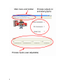
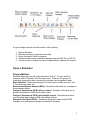
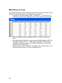
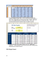
SimWare Pro
User’s Manual
Copyright © 2003 Digital Computations Inc.All Rights
Reserved. Unauthorized Duplication Prohibited By Law.
1
Table of Contents
USING SIMWARE ................................................................................................ 5
SimWare..................................................................................................................... 5
Getting Started ....................................................................................................... 5
Overview............................................................................................................ 5
Open a Simulator ............................................................................................... 7
Start Simulator ................................................................................................... 8
Export Data ........................................................................................................ 8
Reset Current..................................................................................................... 8
Memorize ........................................................................................................... 9
Clear Memorized................................................................................................ 9
Toolbar........................................................................................................................................9
Statistical Analysis ............................................................................................. 10
Cpk Analysis .................................................................................................... 10
Control Chart.................................................................................................... 10
Histogram ........................................................................................................ 10
DOE Analysis .........................................................................................................................10
DOE Analysis ........................................................................................................ 11
DOE Wizard Step 1.......................................................................................... 11
DOE Wizard Step 2.......................................................................................... 11
DOE Wizard Step 3.......................................................................................... 11
DOE Wizard Step 4.......................................................................................... 11
Export DOE Data ...................................................................................................................12
SPC XL ..................................................................................................................... 13
DOE PRO ................................................................................................................ 13
DFSS Master ......................................................................................................... 13
SIMULATOR EXERCISES ................................................................................. 13
Simulator Exercises .......................................................................................... 14
Solutions ............................................................................................................. 14
2
Basic Stats .............................................................................................................. 17
Basic Stats Simulators ..................................................................................... 17
t Test (Oil Refinery).......................................................................................... 17
F Test (Data Entry) .......................................................................................... 18
Correlation (Call Center) .................................................................................. 18
Scatter Plot (Kiln) ............................................................................................. 19
Control Chart (Car Compactor) ........................................................................ 19
Summary Stats (Delivery Time) ....................................................................... 20
Box Plot (Phone Cover) ................................................................................... 20
Show Me How (Basic Stats) ............................................................................ 21
t Test (Show me how) ................................................................................... 21
F Test (Show me how) .................................................................................. 23
Correlation (Show me how)........................................................................... 26
Scatter Plot (Show me how).......................................................................... 29
Control Chart (Show me how)....................................................................... 31
Control Chart (Show me how #2).................................................................. 32
Summary Stats (Show me how).................................................................... 33
Box Plot (Show me how) ...........................................................................................................34
Measurement System Analysis ................................................................ 36
Measurement System Analysis Simulators...................................................... 37
Measurement Error (MSA) ............................................................................... 37
Compressor (MSA) .......................................................................................... 37
Micrometer (MSA)............................................................................................ 38
Visual Clarity (MSA)......................................................................................... 38
Visual Clarity Advanced (MSA) ........................................................................ 38
Show Me How (MSA)....................................................................................... 39
MSA (Show me how) ..................................................................................................................40
DOE (Single Output) ........................................................................................ 42
DOE (Single Output) Simulators ...................................................................... 43
Airline Simulation (DOE) .................................................................................. 43
Commercial Profit (DOE) ................................................................................. 43
Space Ship Thrust (DOE) ................................................................................ 43
Temperature Control (DOE)............................................................................. 44
Hydraulic Hammer (DOE) ................................................................................ 44
Blood Analysis (DOE) ..........................................................................................................44
Broadcast News (DOE) ........................................................................................44
Vial Filling (DOE) ...................................................................................................................44
3
DOE (Multiple Output) ..................................................................................... 45
DOE (Multiple Outputs) Simulators .................................................................. 45
Restaurant (DOE) ............................................................................................ 45
Space Shuttle Main Engine (DOE)................................................................... 45
Vehicle Impact Safety ..........................................................................................................45
DFSS (Design for Six Sigma) .................................................................... 45
DFSS Simulators ............................................................................................. 46
Resistor (DFSS)............................................................................................... 46
Stun Gun (DFSS)............................................................................................. 47
Nuclear Reservoir (DFSS) ............................................................................... 47
Spark Plug Design (DFSS) .............................................................................. 48
Washing Machine (DFSS) ............................................................................... 49
Washing Machine Advanced (DFSS) .............................................................................50
MEMORIZE DATA.............................................................................................. 51
STATISTICAL ANALYSIS ................................................................................. 51
4
Using SimWare
SimWare
Welcome to SimWare by Digital Computations, Inc. SimWare is a statistical
simulator which allows you to practice analyzing data and taking corrective action
as a result of the analysis.
For information about how to get started go to the Overview page.
To learn about the toolbar go to the toolbar page.
For practice exercises go to the exercise page.
Getting Started
Overview
SimWare is a statistical simulator which allows you to practice analyzing data
and taking corrective action as a result of the analysis.
SimWare will allow you to perform a variety of analysis such as t-Test, F Test,
Measurement System Analysis, and primarily Design of Experiments (DOE).
When you first start SimWare you will need to open a simulator from the
"Simulator" menu item. At this point the screen is divided into three main areas.
The top area is the toolbar/menu bars, the center area is were the animation and
analysis is performed, and the bottom area is where you can control the inputs to
the simulation.
5
6
A typical usage scenario would be similar to the following:
1.
2.
3.
4.
5.
Open a Simulator.
Start the simulator to generate some data.
Export the data to Excel for analysis.
Analyze the data using a statistical program such as DOE Pro or SPC XL.
Use the results to change the inputs (if applicable) to optimize the outputs.
Open a Simulator
Primary Method
SimWare ships with over 25 quality simulators "built in". To open a built in
simulator select "Simulator" from the main menu. There are five groups of
simulators arranged by what concepts the simulators are designed to teach.
Basic Statistics - Simulations designed to teach basic concepts such as t Test,
F Test, Summary Stats, etc.
Measurement System Analysis (MSA) - Simulations that allow you to analyze a
measurement system.
Design of Experiments (DOE) with one output - Simulators that allow you to
perform and analyze a DOE with a single output.
Design of Experiments (DOE) with multiple outputs - Simulators that allow
you to perform and analyze a DOE with multiple outputs.
Design for Six Sigma (DFSS) - Simulators designed to demonstrate DFSS
concepts such as parameter design and tolerance allocation.
7
WebService
You can also download simulators from the SimWare Pro WebService by
selecting "File" - "WebService" from the menu bar. The WebService is intended
to allow users to create their own simulators and share them with others. Note
that simulators that are shared in this manner are not by Digital Computations
and are therefore not supported.
Open
SimWare supports opening a simulator from a file (with a .simw extension). This
allows you to create and share simulators with others. Note that simulators that
are shared in this manner are not by Digital Computations and are therefore not
supported.
Start Simulator
SimWare supports two methods for running a simulation.
Continuous Simulation
To start a continuous simulation, select "Start" - "Speed" and then the desired
speed from the menu bar. The simulation will run until you stop the simulation by
selecting "Start" - "Speed" - "Stop" from the menu bar.
Generating a Specific Number
SimWare allows you to generate 1, 25, 100, or 1000 iterations and then stops
automatically. To generate a specific number, select "Start" - "Generate" followed
by the desired number from the menu bar.
Export Data
The data that is generated by your simulator can be exported to Excel, the
clipboard, a comma separated file, or a tab delimited file. Exporting to Excel
requires that MS Excel version 2000 or later be installed. To export data, select
"Export Data" followed by the desired format from the menu bar.
What gets exported?
If you are exporting to Excel, then both the current data and memorized data (if
any exist) will be exported to a workbook in Excel.
If you are exporting to the clipboard, a comma separated file, or a tab delimited
file then you must export the current data and memorized data separately.
How do I export the results of a DOE?
See Export DOE Data
Reset Current
As you generate data, the data is stored in the data grid and the analysis is
performed by any statistical tools that you have started. If you would like to reset
8
the analysis and delete the data from the grid, select "Control" - "Reset Current"
from the main menu bar.
Reset Current does not affect any memorized data. To delete the memorized
data you need to Clear Memorized.
Memorize
In many cases it is desirable to compare previous data with the current data. To
assist in this, SimWare allows you to "memorize" the current data by selecting
"Control" - "Memorize" from the main menu.
y Any data in the Data Grid will be placed on a new tab entitled "Memorized
Data".
y The current Cpk curve will be represented by a single line and the
statistics for the memorized data will be retained.
y The current Histogram will be reflected in different colors and the statistics
for the memorized data will be retained.
y There is no visual indication of memorized data on the control chart;
however, the statistics will
y be retained.
Clear Memorized
After you have memorized data you can clear the data by selecting "Control" "Clear Memorized" from the main menu.
Toolbar
The toolbar at the top of SimWare is designed to allow rapid access to the
majority of SimWare's features.
9
Statistical Analysis
Cpk Analysis
To start the Cpk Analysis, select "Stats" - "Cpk" from the main menu.
Cpk Analysis will display a graphical bell curve and associated statistics. The
area out of specification will be red, while the area in spec will be blue. Note, you
must have variation in the data in order to get a Cpk analysis.
When you start the Cpk Analysis you will get a new window for each output. The
statistics calculated are:
y Mean
y Standard Deviation
y Cp
y Cpk
y DPM (defects per million)
y Sigma Capability
Control Chart
To create a control chart, select "Stats" - "Control Chart" from the main menu.
When you first create the control chart it will plot the data until it has enough data
to calculate the control limits (the default is 25 plotted points). When the control
limits have been calculated, they will not be reset until you reset the current data.
You can change the subgroup size, the way out-of-control checking is performed
for both the Xbar and R chart, and the number of plotted points required to
establish the control limits by selecting these options on the right side of the
window.
Histogram
To create a histogram, select "Stats" - "Histogram" from the main menu.
The histogram window will appear and create a histogram of any further data
generated after initial creation. The mean, standard deviation, Cp, Cpk, and DPM
are also calculated concurrently.
DOE Analysis
To start a DOE, select "Stats" - "DOE" from the main menu.
The DOE functionality in SimWare enables you to quickly create designs and
generate the associated dependent data (output). The analysis of the DOE must
be performed in a DOE software package such as DOE Pro.
When you start the DOE Analysis, the DOE Wizard will start and lead you
through the process of determining what design you would like to run, selecting
the factors for the design, selecting the lows and highs, and determining the
number of replicates.
When you have completed the wizard, a new window will appear with the
10
independent data (inputs) and dependent data (outputs). This can be exported to
Excel for analysis.
DOE Analysis
DOE Wizard Step 1
The first step in the DOE Wizard is to select the type design that you would like
to create. You may select from a variety of 2 or 3 level designs that are built into
SimWare. To change from a 2 to 3 level design, use the radio button on the left
side of the window.
SimWare will only show you designs which the current simulator supports. For
example, if the current simulator has three inputs then you will not be given an
option of a 24 full factorial.
After selecting the desired design select "Next" and proceed to step 2.
DOE Wizard Step 2
After selecting the desired design, you may be prompted to select the factors you
wish to include in the DOE. Note: If the design you chose requires all of the
factors in the current simulator, you will not see step 2.
Select the factors using the check box next to the name of each factor and select
"Next" to continue to Step 3.
DOE Wizard Step 3
Now that you have selected the factors for the DOE, you need to determine what
the range for each factor will be. The default range is low and high for the
extremes in each factor; however, you may change this value to any value that is
possible given the design you have chosen.
It is possible to choose values that are not possible and if you do you will get an
advisory message. For example, if you have a three level design and you have a
factor which is marked as (Integer Only), then a low of 1 and a high of 4 would
not be possible because the center point would be 2.5 which is not an integer.
However, a low of 1 and a high of 5 would be possible because the center point
would be 3, which is allowed.
You are now ready for Step 4.
DOE Wizard Step 4
The final step is to select the number of replicates. You may have between 1 and
20 replicates for the DOE.
When done, select "Finish" and SimWare will create the DOE Design for you.
You will also be asked if you would like SimWare to generate the replicates for
you. If you indicate "Yes" then the dependent data will be filled according the
design.
At this point you should export the data to Excel for analysis in a software
11
package such as DOE Pro.
Export DOE Data
If you have created a DOE in SimWare, then while the DOE output is visible a
new menu item will be available called "DOE Control". This menu item allows you
special control over the DOE options in SimWare. To export the data, select
"DOE Control" - "Export", then the desired format. You have the option of
exporting the DOE data in either DOE Pro or stacked formats.
Excel (DOE Pro Format)
The entire DOE, including the dependent and independent data, the formatting,
and the coding will be exported into a DOE Pro design sheet which is ready for
analysis. You must have Excel 2000 or later installed to export to Excel.
Excel (Stacked)
The dependent and independent data will be exported into Excel in the format
that is usually required by DOE software other than DOE Pro. You must have
Excel 2000 or later installed to export to Excel.
How do I export the contents of the Data Grid?
See Exporting Data
12
SPC XL
SPC XL is a Microsoft Excel add-in which gives users powerful
yet easy-to-use SPC (Statistical Process Control) capabilities.
From within Excel you will be able to access many tools for
statistical analysis, including Control Charting, Cpk analysis,
Histograms, Paretos, MSA, and much more. The data analysis
in this help system was performed using SPC XL.
For more information visit
http://www.sigmazone.com/spcxl.htm
DOE PRO
DOE PRO XL is the ultimate in Design of Experiments
packages. Multiple response capability coupled with advanced
analysis and optimization features enables you to take control of
your experiments, all from within Microsoft Excel. The data
analysis in this help system was performed using DOE Pro.
DOE PRO XL is an Excel add-in which gives users powerful yet
easy-to-use DOE (Design of Experiments) capabilities. From
within Excel you will be able to create designs, analyze designs
using multiple regression, plot results, optimize, and predict.
For more information visit
http://www.sigmazone.com/doepro.htm.
DFSS Master
DFSS Master is an Excel add-in which facilitates Design for Six
Sigma initiatives. Features include Monte Carlo simulation,
Design Scorecards, Tolerance Allocation tables, Parameter
Design for factor optimization, and much more.
For more information visit
http://www.SigmaZone.com/dfssmaster.htm
Simulator Exercises
13
Simulator Exercises
In order to facilitate the learning of statistical concepts, problems or scenarios
around each simulator are available. The exercises allow you to practice using
SimWare and your statistical software. In most cases, you must have statistical
software to perform the analysis such as SPC XL, DOE Pro, and DFSS Master.
Basic Stats Simulators - Exercises designed around basic statistical concepts
such as t-Test, F Test, Correlation, Scatter Diagrams, Box Plots, and Summary
Stats.
Measurement System Analysis Simulators - Exercises designed to practice
analyzing and evaluating measurement systems using MSA.
DOE (Single Output) Simulators - Exercises that allow you to perform a DOE on
a simulated process to include optimization and confirmation.
DOE (Multiple Outputs) Simulators - Exercises designed to practice DOE on
processes that have more than one output (response).
DFSS Simulators - Exercises which enable you to practice more advanced
techniques such as Robust Design and Tolerance Allocation. Most of these
simulators require a good foundation in DOE for completion.
Solutions
This section contains the underlying models for some of the simulators so you
can compare your results with those in the Simulator. Note that your solution will
not match this solution exactly.
Measurement System Simulations
DOE Single Output Simulations
DOE Multiple Output Simulations
Design for Six Sigma Simulations
⎯⎯⎯⎯⎯⎯⎯⎯⎯⎯⎯⎯⎯⎯⎯⎯⎯⎯⎯⎯⎯⎯⎯⎯⎯⎯⎯⎯⎯⎯⎯⎯⎯⎯⎯⎯⎯⎯⎯⎯⎯⎯⎯⎯⎯⎯⎯
Measurement System Simulations
Compressor
Operator #1 is reading the display to the tenths digit. Operator #2 is reading the
display to the hundredths digit. This artificially deflates the standard deviation of
Operator #1, which can be easily seen by creating a Cpk diagram and running
100 simulations. Operator #1 doesn't have sufficient discrimination.
Micrometer
The primary contributor to variation is repeatability with reproducibility playing a
small roll also.
Visual Clarity
Reproducibility accounts for more than 90% of the total variation. Operator #2
consistently measures less than Operator #1.
⎯⎯⎯⎯⎯⎯⎯⎯⎯⎯⎯⎯⎯⎯⎯⎯⎯⎯⎯⎯⎯⎯⎯⎯⎯⎯⎯⎯⎯⎯⎯⎯⎯⎯⎯⎯⎯⎯⎯⎯⎯⎯⎯⎯⎯⎯⎯
DOE Single Output Simulations
Airline Simulation
14
Minutes Late = 30-28*Num Employees
The standard deviation decreases when NumJets increases.
Commercial Profit
Profit = 1000 + 250 * $ Advert + 100 * $ Training
The standard deviation decreases when Percent Stocked increases.
Space Ship Thrust
Thrust = 500+266*Muon Flux-134*Plasma
The standard deviation decreases with Test Pilot 2.
Temperature Control
Temp = 500-132*Ionization Rate+67*NaCl2+22*Ionization Rate*Oxygen Ratio34*NaCl2*MgBer
The standard deviation decreases when the Nitrogen Level decreases.
Hydraulic Hammer
Error = 100-36*Fluid Type+41*Hyd Pressure+21*Hammer Friction*Surface Temp
The standard deviation decreases when Rivet Density decreases.
The Hammer Friction*Surface Temp interaction is difficult to pick out in a
screening design, which is common if an interaction is significant but neither of
the main effects in the interaction is significant. If you set Rivet Density at the low
and then run a 25-1 with the remaining factors the interaction will be significant in
the DOE.
Blood Analysis
Optical Density = 1100+300*Reagent Conc.+160*pH-50*Reagent
Conc.2+35*Reagent Conc.*pH+75*Incubation Time
The standard deviation decreases with Substrate Type 2.
Broadcast News
Audience Size = 60+20*Edit Time+10*Num Cameras
The standard deviation decreases with the "Standard Plus" edit method (i.e., Edit
Method = Standard Plus).
Vial Filling
Volume = 35+2.4*Active Press-1.2*Active Press2-5.4*Inert Press+2.4*Inert
Press2+3.2*Flow Ratio-1.3*Nozzle Diameter-5.2*Nozzle Diameter2+0.8*Active
Press*Inert Press+4.5*Active Press*Nozzle Diameter
The standard deviation decreases when Inert Pressure decreases. Note: Inert
Pressure also shifts the mean.
⎯⎯⎯⎯⎯⎯⎯⎯⎯⎯⎯⎯⎯⎯⎯⎯⎯⎯⎯⎯⎯⎯⎯⎯⎯⎯⎯⎯⎯⎯⎯⎯⎯⎯⎯⎯⎯⎯⎯⎯⎯⎯⎯⎯⎯⎯⎯
DOE Multiple Output Simulations
Restaurant
Minutes till Order = 6-1.4*Num Cash Registers-.8*Tables Per Waiter-.4*Num
Cash Registers*Tables Per Waiter
Minutes till Drinks = Minutes_till_Order+6-1.2*Tables Per Waiter-.8*Music
15
Type+.7*Tables Per Waiter*MusicType
Minutes till Entree = Minutes_till_Drinks+7-2.9*NumChefs
The standard deviation is not affected by the model.
Space Shuttle ME
Left Engine = 300+58*Core Temp-68*Nozzle Temp+35*Chamber Press+75*Left
Temp+44*NozzleTemp2-24*CoreTemp231*CoreTemp*NozzleTemp+26*Chamber Press*Left Temp
The Left Engine standard deviation decreases with an increase in Neutrinos.
Right Engine = 300+45*CoreTemp-58*NozzleTemp+55*Chamber
Press+65*Right Temp+34*Nozzle Temp2-34*Core Temp2-41*Core Temp*Nozzle
Temp+36*Chamber Press*Left Temp
The Right Engine standard deviation decreases with an increase in Neutrinos.
Vehicle Impact Safety
Triaxial Acceleration = 18-.8*Cross Support Dia-.7*Box Dia-2.3*Beam Angle.8*Box Dia*Beam Angle+.8*Cross Support Dia*Box Dia
The Triaxial Acceleration standard deviation decreases with an increase in Box
Diameter.
Rib Compression = 14-.7*Cross Support Dia-2.1*Vert Support Dia-1.2*Box Dia1.1*Beam Angle-.5*Box Dia*Beam Angle+.84*Cross Support Dia*Vert Support
Dia
The Rib Compression standard deviation decreases with an increase in Box
Diameter.
Design Cost = 140+27*Cross Support Dia+56*Vert Support Dia+110*Box Dia
The Design Cost standard deviation is not affected by the model.
⎯⎯⎯⎯⎯⎯⎯⎯⎯⎯⎯⎯⎯⎯⎯⎯⎯⎯⎯⎯⎯⎯⎯⎯⎯⎯⎯⎯⎯⎯⎯⎯⎯⎯⎯⎯⎯⎯⎯⎯⎯⎯⎯⎯⎯⎯⎯
Design for Six Sigma Simulations
Resistor
The equation for impedance is on the animated graphic and is (R1*R2)/(R1+R2).
Stun Gun
Pulse Watts = 27500+2400*Power-125*Freq + 2600*Power*Freq
Nuclear Reservoir
Water Level = 700+50*Plug Press+122*Bellow Press-66*Ball Press+100*Water
Temp+96*Water Temp*Plug Press-33*Bellow Press*Ball Press
An interaction causes water temp variation to induce significant variation in water
level if the PlugPress is high (50).
Spark Plug Design
KV to Spark = 25-2.8*Groove Angle+2*Welding Pwr+1*Laser Angle1.7*Rotational Speed-1.6*Rotational Speed2+2.1*Rotational Speed*Groove
Angle
The standard deviation is lowest with Rotational Speed in central setting (5) due
to the quadratic. Very difficult to pick up.
16
Washing Machine Design
Cleaning Effectiveness = 331+55*Water Height+45*Angle-48*Water
Height*Agitator Angle+20*Water Height2-60*Agitator Angle2+55*Agitator
Width+39*Drum Accel
Energy Consumption = 250+88*Accel+44*Agitator Width+22*Agitator
Angle+19*Accel*Agitator Angle
Basic Stats
Basic Stats Simulators
SimWare includes 7 simulators that are designed to teach basic statistical tools.
t Test (Oil Refinery)
F Test (Data Entry)
Correlation (Call Center)
Scatter Plot (Kiln)
Control Chart (Car Compactor)
Summary Stats (Delivery Time)
Box Plot (Phone Cover)
t Test (Oil Refinery)
You are in the employ of a company that owns two oil refineries. Both refineries
operate using electric dehydration and desalinization to refine the low-sulfur
crude that is provided by your customers. One of your key metrics is the number
of barrels of crude that can be refined per day.
The plant manager of the Northern Plant has proposed that his new method of
handling waste byproducts has enabled the Northern Plant to produce more
barrels of oil than the Western Plant. Since the two plants are identical in every
other way, you decide to do a t Test to determine if there is a statistical difference
between the two plants.
Problem #1: Perform a t-Test on the data from each plant (with the Crude
Price = $20 per barrel) to determine if there is a difference between the
Northern and Western Plants.
Since the number of barrels that can be produced per day is dependent on the
price of crude, you decide to withhold your judgement and wait until the price of
crude increases to $30 per barrel.
17
Problem #2: Change the price to $30 per barrel and redo the analysis.
Show me how
F Test (Data Entry)
Your company takes insurance claims via telephone in centralized call centers
for multiple insurance brokers. Each broker has slightly different requirements in
terms of the fields (data for each call) to be collected. Over time, this has lead to
multiple screen formats to which the operator must adapt. Your project is to make
these forms as similar as possible to make the data entry easier on the operator.
Problem #1: Perform an F-Test to determine if there has been a significant
change in the standard deviation in the time required to complete a record.
Show me how
Problem #2: Perform a t-Test to determine if there has been a significant
change in the mean.
Problem #3: The goal is for all operators to finish a call in less than 90
seconds. Based upon the information you have gathered in Problems 1 and
2, predict if the process capability (Cpk) will be improved by implementing
the project.
Problem #4: Perform a Cpk analysis and compare the results to your
prediction.
Correlation (Call Center)
You are the manager of a small call center which handles inbound inquiries from
a variety of vertical industries. One of your key metrics is the time customers
spend on hold waiting for a customer service representative. Most of your
contracts require that this be no longer than 70 seconds. You have a variety of
factors in your control, including the number of operators, the number of
customer service representatives, and the number of lines (trunks).
Problem #1: Start the simulation and randomly change the # of operators, #
of customer service reps, and # of lines. If you start a continuous
simulation on medium speed, you can change these inputs while the
simulation is running. Export the data and perform a correlation analysis in
a statistical software package such as SPC XL. Which inputs are correlated
with time on hold?
Show me how
Problem #2: What does a positive vs. a negative correlation coefficient
mean?
Problem #3: Where should you set the inputs in order to reduce the time on
hold?
18
Scatter Plot (Kiln)
As the manager in a small arts and crafts store you are responsible for the
results of the glazing process. In order to attract customers, you need to ensure
that your glazing process provides a glaze thickness of at least 4.2 mm but no
more than 4.8mm.
You suspect that the temperature of the kiln is important in the thickness of the
glaze.
Problem #1: Start the simulation in continuous mode (medium speed is
best) and slowly increase the Kiln Temp from the minimum to the
maximum. Export the data and create a scatter diagram. Does changing the
Kiln Temp change the Glaze Thickness?
Show me how
Problem #2: Based upon your scatter diagram, what is the optimal kiln
temperature to produce the desired glaze thickness?
Problem #3: Create a Cpk diagram in SimWare, set the kiln to the
temperature you chose in problem #2, and confirm your analysis.
Control Chart (Car Compactor)
As a car compacting fiend, you are obsessed with the quality of your car
compaction. As such you have the ability to adjust the mean and standard
deviation of the resulting thickness at will. However, you would like to investigate
if your process is in statistical control.
Problem #1: Leave the process mean and standard deviation (the inputs) at
their default settings and start a control chart until the control limits have
been established (leave the sub group size set at the default of one). What
are the center, UCL, and LCL values for the X/Xbar chart? Based upon the
process mean and standard deviation, do those numbers make sense?
Show me how
Problem #2: Run the simulation for 100 more data points without adjusting
the mean or standard deviation. Do you see any out-of-control conditions
(red points)? If you did, why would you see out of control conditions if the
mean and standard deviation didn't change?
Problem #3: Adjust the mean 1.5 standard deviations to the right (265) and
generate 100 more data points. Did the number of out-of-control conditions
increase?
Problem #4: Change the subgroup size (in upper right corner) to 4. This will
cause the control limits to be reset. Generate 100 more data points to
19
generate the control limits. What are the center, UCL, and LCL values? How
do these values compare with the control limits when the sub group size
was 1? Why is there a difference?
Show me how
Summary Stats (Delivery Time)
You are responsible for the shipping of products from the small parts facility in
your company. You suspect a problem in shipping and as such you would like to
collect some data and get a baseline for shipping time performance.
Problem #1: Run the simulation and export to Excel for analysis. Analyze
the shipping time and calculate the summary statistics (mean, standard
deviation, confidence intervals for the mean, etc).
Show me how
Problem #2: What is the average shipping time? What is the standard
deviation?
Problem #3: Calculate the following:
y Mean shipping time plus two standard deviations
y Mean shipping time minus two standard deviations
What percent of shipments should fall between these two numbers?
Problem #4: What is the 95% confidence interval for the mean (upper and
lower limit)? Compare these numbers to the mean +/- 2 standard
deviations. Should the numbers be the same, and if not, what is the
difference?
Box Plot (Phone Cover)
You are responsible for designing the sliding phone cover for your company's
next mobile phone. One of the key metrics for the phone is the force required to
actuate (slide) the cover from the closed to the open position. After a couple of
months of development, there are four competing designs.
Problem #1: Generate at least 25 data points and export the data to Excel
for analysis. Create a Box Plot of the resulting data.
y Which design requires the most force for actuation (on average)?
y Which design requires the least force of actuation (on average)?
y Which design has the most variation?
y Which design has the least variation?
Show me how
Problem #2: Customer surveys indicate that customers prefer the "feel" of
a phone if the force required is between 1 and 2 newtons. Based upon the
box plot, which phone appears to meet this customer specification the
best?
20
Problem #3: Create a Cpk analysis and confirm which phone design has
the best process capability.
Show Me How (Basic Stats)
t Test (Show me how)
This "show me how" requires SPC XL which is a separate product from SimWare
Pro. For more information click here.
y
y
y
y
After opening SimWare, generate 25 data points by selecting "Start" "Generate" - "25" from the main menu.
Export the data to Excel by selecting "Export Data" - "Excel" from the main
menu.
Select the columns entitled "northern_plant" and "western_plant".
From the Excel menu select "SPC XL" - "Analysis Tools" - "t Test Matrix
(Mean)". If you do not see the "SPC XL" menu item it means you need to
start SPC XL.
21
y
The first screen SPC XL will present you with will confirm the range
selected.
y
The next will ask if your groups are in rows or columns.
y
The result will be created on a new worksheet.
The simplest way to interpret a pvalue is that we have (1-pvalue)*100%
confidence that the means are not equal. In this case, we are only 44% confident
that the means are not equal. Had the p-value been .1 then we would be 90%
confident that the means are not equal.
The second part of the problem asks what happens if you change the crude
price to $30 per barrel.
22
y
Change the crude price to $30
y
Reset the current data by selecting "Control" - "Reset Current" from the
main menu. This will remove the previous data from the data grid.
y
Now just follow the instructions from the start of this section (start by
generating 25 data points) and you should get a result similar to the
following.
The p-value now shows "0.0" which means that we are over 99.9% confident that
the means are different.
When the Crude Price is $20 per barrel, there is no difference in the output from
the northern and western plants. However, when the crude price is $30 there is a
difference between the two plants.
Further inquiries of interest would be to determine if there is a difference when
the crude price is $21 per barrel. If not, what if you generate 100 data points
instead of 25? Why would the number of data points affect the analysis?
F Test (Show me how)
y
Ensure that the Project Status is set to "Pre-Project".
y
Generate 25 data points by selecting "Start" - "Generate" - "25" from the
23
y
y
y
y
y
y
y
24
menu bar
Memorize this data by selecting "Control" - "Memorize" from the menu bar.
Reset the current data by selecting "Control" - "Reset Current" from the
menu bar.
Change the Project Status to "Project Complete"
Generate 25 data points by selecting "Start" - "Generate" - "25" from the
menu bar.
Export the data to Excel by selecting "Export" - "Excel" from the menu bar.
The memorized and current data will be exported to Excel on separate
worksheets.
Copy the current data to a new worksheet and give it the column name
"Project Complete". Copy the memorized data to the new worksheet and
give it the column name "Pre-Project". Select the two columns including
the column headings.
y
y
y
Select "SPC XL" - "Analysis Tools" - "F Test Matrix (Std Dev)" from Excel's
menu. If you don't see the SPC XL menu item you need to start SPC XL.
The first window will ensure you have the correct data selected. Ensure
that the range of cells is correct and press "Ok".
Next, you need to tell SPC XL that the data is in Columns by clicking on
the button "Data in Columns".
25
y
SPC XL calculates the results and give you the p-value.
You have (1-pvalue)*100% confidence that the variances are not equal. In this
case, since the p-value is .000931 you are over 99.9% confident that the
variances are not equal.
Further items to explore
Would the answer change if you only generated 10 data points? Why would
fewer data points change the results? Did the project "improve" the process?
Correlation (Show me how)
y
y
26
Start the simulation by selecting "Start" - "Speed" - "Medium" from the
main menu.
While the simulation is running, change the inputs to random values. Make
sure you go to the extreme minimum and maximum values for the inputs
while you are changing the inputs. Make the changes random; don't
change all of the inputs to the high values and then return all of them to
the low. Move some up and others down while the simulation is running.
y
y
y
y
y
After you have generated about 100 data points, stop the simulation by
selecting "Start" - "Speed" - "Stop" from the main menu.
Export the results to Excel by selecting "Export" - "Excel" from the main
menu.
Select all the data (including the column titles)
Select "SPC XL" - "Analysis Tools" - "Correlation Matrix" from Excel's
menu bar. If you don't see the SPC XL menu you need to start SPC XL.
The first step is to ensure that you have selected the correct data range.
Click Ok to continue.
27
y
Since the data is in columns, click on the "Data in Columns" button.
y
SPC XL calculates the correlation and gives us the results.
The correlation coefficient for # Operators vs. time is -.997. This indicates a
strong negative correlation. Anything below -.7 and above .7 is colored red by
SPC XL to indicate a strong correlation. This indicates that as # Operators is
increased time will decrease.
Further Items to Explore
28
Is it possible that two of the inputs would end up being highly correlated?
Why is the diagonal of the correlation matrix all 1.0?
If this were your process, where would you set the inputs?
Scatter Plot (Show me how)
y
y
Start the simulation by selecting "Start" - "Speed" - "Medium" from the
main menu.
While the simulation is running slowly, increase the inputs until you reach
the maximum of 1200 degrees.
y
y
Export the data by selecting "Export" - "Excel" from the main menu.
In Excel, select the data including the column headings.
y
Select "SPC XL" - "Analysis Diagrams" - "Scatter Plot" from Excel's menu.
29
y
30
If you do not see the SPC XL menu item you need to open SPC XL.
Ensure that the selected data range is correct and press the "Next >>"
button.
y
Indicate that the data is in columns by clicking on the "Data in Columns"
button.
y
SPC XL creates the scatter plot.
The high R2 value indicates that the model is a good fit. As the Kiln temperature
increases, so does the thickness.
Further Items to Explore
What is the difference between R2 and a p-value?
What are the minimum and maximum values for R2?
Control Chart (Show me how)
y
y
y
Start a control chart analysis by selecting "Stats" - "Control Chart" from the
main menu.
Generate 25 data points by selecting "Start" - "Generate" - "25" from the
main menu.
The control chart should add data until it has sufficient data to establish
the control limits.
31
y
Expand the tree on the right of the control chart to see the value of the
control limits.
In this case, the UCL is 275 and the LCL is 222 with the center at 248.
Further Items to Explore
Export the data and repeat the analysis in SPC XL.
Will the control limits always be the same? If not, why would they change?
Control Chart (Show me how #2)
y
32
Select the drop down box and change the value to 4.
Summary Stats (Show me how)
y
y
y
y
y
Generate 25 data points by selecting "Start" - "Generate" - "25" from the
main menu.
Export the data to Excel by selecting "Export" - "Excel".
In Excel, select the data using the mouse.
Select "SPC XL" - "Analysis Diagrams" - "Summary Stats (Dot Plot)" from
Excel's menu. If you don't see the SPC XL menu item, then you need to
start SPC XL.
Confirm the range is correct by clicking on "Next >>".
33
y
SPC XL analyzes the results and creates the summary statistics.
Box Plot (Show me how)
y
y
y
34
Generate 25 data points by selecting "Start" - "Generate" - "25" from the
main menu.
Export the data to Excel by selecting "Export" - "Excel".
In Excel, select the data using the mouse.
y
y
y
Select "SPC XL" - "Analysis Diagrams" - "Box Plot" from Excel's menu. If
you do not see the SPC XL menu item you need to start SPC XL.
Ensure the data range is correct and click "Next >>".
Our data sets are in columns, so select the radio button "Data sets in
Columns" and press "Next".
35
y
SPC XL creates the Box Plot.
Measurement System Analysis
36
Measurement System Analysis Simulators
Measurement Error (MSA) - A simulator that provides a "True Value" and
"Measured Value" output. Demonstrates the impact of a poor measurement
system in terms of process capability.
Compressor (MSA) - Two operators with a single replicate.
Micrometer (MSA) - Three operators with two reps per operator.
Visual Clarity (MSA) - Two operators with two reps per operator.
Visual Clarity Advanced (MSA) - Same as the Visual Clarity simulation but with
inputs that allow you to change the variance components of the MSA.
Measurement Error (MSA)
The purpose of this simulator is to demonstrate the impact of a poor
measurement system on the capability of the process. The simulator has two
outputs, the "True Value" and the "Measured Value". The true value represents
the actual measurement before any measurement error has been introduced.
The measured value represents the measurement after the measurement error
has been introduced. In most applications you can not really know the "true
value"; however, you can estimate the variation that is introduced by the
measurement system.
Exercise #1: Start a Cpk analysis for this simulator and generate 25 data
points with the default inputs. What is the Cpk of the "True Value" vs. the
"Measured Value"?
Exercise #2: Reset the data and increase the Measurement Standard
Deviation to a value of 6. Again, compare the "True Value" vs. the
"Measured Value".
Exercise #3: Reset the data and change the Measurement Bias to a value of
-10. Compare the Cpk of the true vs. measured values.
Exercise #4: Can a poor measurement system decrease the Cpk of a
process? Can a part that is in reality good be classified as bad? Can a bad
part be classified as good? If your process is operating with a poor Cpk,
how can you tell if the problem is primarily the measurement system or the
process?
Compressor (MSA)
Two operators are concurrently reading the pressure of a compressor.
Exercise #1: Perform a measurement system analysis on the two operators.
What appears to be the problem?
37
Micrometer (MSA)
In this simulation you have three operators who all measure the same part twice.
The USL is 13 and the LSL is 7.
Exercise #1: Perform a MSA analysis. What percent of the variation is being
caused by the following components?
y Part-to-Part
y Repeatability
y Reproducibility
If this was your process, what would you do first in order to increase the
capability?
Show me how
Exercise #2: Change the process mean (the only input) to a value of 11 and
repeat the analysis.
Visual Clarity (MSA)
Two technicians perform a visual clarity analysis of a sample without the use of a
Secchi Disk (rapid testing). You have set up a MSA so that the analysis is
performed twice by both operators on the same sample. The sample is then
measured four times by highly qualified operators using a more precise method
(a Secchi Disk). The average of the four measurements using the Secchi Disk
are the reference values.
Exercise #1: Perform a MSA analysis. What percent of the variation is being
caused by the following components?
y Part-to-Part
y Repeatability
y Reproducibility
Is there any Bias in this measurement system?
If this was your process, what would you do first to increase the capability?
Exercise #2: Change the process mean (the only input) to a value of 11 and
repeat the analysis.
Visual Clarity Advanced (MSA)
This simulator is identical to the Visual Clarity simulator with the addition of inputs
which allow you to experiment with various factors. The following inputs are
available that can be changed:
y Process Mean
y Process Standard Deviation
y Operator 1 Accuracy
y Operator 1 Repeatability
38
y Operator 2 Accuracy
y Operator 2 Repeatability
The process mean and standard deviation control the distribution of the
"Reference Measurement".
The accuracy of the measurement represents the difference an operator will
have on average from the reference measurement. For example, if you set the
accuracy to 0 the operator will be (on average) the same as the reference value.
An accuracy of 1.5 would make the operator be (on average) 1.5 units greater
than the reference value.
The operator repeatability directly controls the repeatability standard deviation for
each operator.
Exercises: Using the provided controls, change the values of the accuracy
and repeatability and perform a MSA.
Show Me How (MSA)
39
MSA (Show me how)
The following steps are for the Micrometer simulation, but the same steps can be
followed for the Visual Clarity or the Compressor simulations.
y Generate 10 parts by pressing "Start" - "Generate" - "1" ten times or by
starting the simulator and stopping it after 10 parts have been generated.
y
y
y
40
Export the data to Excel by selecting "Export" - "Excel" from the main
menu.
Now that the data is in Excel, you must create a MSA template in SPC XL
for analysis. Select "SPC XL" - "MSA (gage capability)" - "Create MSA
Template" from Excel's menu. If you do not see the SPC XL menu item
then you need to start SPC XL.
Indicate that you have 3 operators, 2 replicates, and 10 parts. Enter 13 for
the Upper Spec Limit and 7 for the Lower Spec Limit.
y
SPC XL will create an empty template to enter your data.
y
Go back to the worksheet that holds the data you exported from SimWare.
Select just the output data WITHOUT the column headings and without
the input column.
41
y
Copy this data by selecting "Edit" - "Copy". Go back to the sheet that
contains the MSA template. Select the cell that corresponds to Operator 1,
Rep 1, Part 1 (Should be cell C12) and select "Edit" - "Paste". When you
are done, the MSA template will look like the following. Do not be
concerned if the lines are overwritten when you paste in the data.
y
You are now ready for the analysis. Select "SPC XL" - "MSA (gage
capability)" - "Anova Analysis" from the menu bar and SPC XL will perform
the Measurement System Analysis.
DOE (Single Output)
42
DOE (Single Output) Simulators
Airline Simulation (DOE)
Commercial Profit (DOE)
Space Ship Thrust (DOE)
Temperature Control (DOE)
Hydraulic Hammer (DOE)
Blood Analysis (DOE)
Broadcast News (DOE)
Vial Filling (DOE)
Airline Simulation (DOE)
A new commuter airline has established on time departures as a primary
business goal. You have been tasked to identify the factors that significantly
affect the time of departure, recommend a method of improvement, and confirm
the results.
After completion of an Ishikawa diagram, the factors selected as most likely to
effect the time of departure are $ spent on training, # of Jets, # of Employees,
and % Overbooked. The output is "Minutes Late" with negative values indicating
that the flight left early.
Exercise #1: Perform a DOE on the four inputs and export the data for
analysis in your DOE software. Which factors shift the mean and/or
standard deviation?
Exercise #2: Based upon the results in your DOE, find optimal values for
the inputs. Enter these values into SimWare and confirm your results.
For more information about DOE Pro visit
http://www.sigmazone.com/doepro.htm.
Commercial Profit (DOE)
Exercise #1: Analyze the process by performing a DOE to determine which
factors shift the mean and/or standard deviation.
Exercise #2: Use the results of the DOE to optimize the output. Confirm
your results by entering the optimal values and running the Cpk Analysis
on the simulator.
Space Ship Thrust (DOE)
Exercise #1: Analyze the process by performing a DOE to determine which
factors shift the mean and/or standard deviation.
Exercise #2: Use the results of the DOE to optimize the output. Confirm
43
your results by entering the optimal values and running the Cpk Analysis
on the simulator.
Temperature Control (DOE)
Exercise #1: Analyze the process by performing a DOE to determine which
factors shift the mean and/or standard deviation.
Exercise #2: Use the results of the DOE to optimize the output. Confirm
your results by entering the optimal values and running the Cpk Analysis
on the simulator.
Hydraulic Hammer (DOE)
Exercise #1: Analyze the process by performing a DOE to determine which
factors shift the mean and/or standard deviation.
Exercise #2: Use the results of the DOE to optimize the output. Confirm
your results by entering the optimal values and running the Cpk Analysis
on the simulator.
Blood Analysis (DOE)
Exercise #1: Analyze the process by performing a DOE to determine which
factors shift the mean and/or standard deviation.
Exercise #2: Use the results of the DOE to optimize the output. Confirm
your results by entering the optimal values and running the Cpk Analysis
on the simulator.
Note: A 3 level design will provide optimal results.
Broadcast News (DOE)
Exercise #1: Analyze the process by performing a DOE to determine which
factors shift the mean and/or standard deviation.
Exercise #2: Use the results of the DOE to optimize the output. Confirm
your results by entering the optimal values and running the Cpk Analysis
on the simulator.
Vial Filling (DOE)
Exercise #1: Analyze the process by performing a DOE to determine which
factors shift the mean and/or standard deviation.
Exercise #2: Use the results of the DOE to optimize the output. Confirm
your results by entering the optimal values and running the Cpk Analysis
on the simulator.
44
Note: A 3 level design will provide optimal results.
DOE (Multiple Output)
DOE (Multiple Outputs) Simulators
Restaurant (DOE)
Space Shuttle Main Engine (DOE)
Vehicle Impact Safety
Restaurant (DOE)
As a small restaurant owner you are responsible for timely delivery of service.
Using the available inputs, reduce the time required for each of the services
provided.
Exercise #1: Analyze the process by performing a DOE to determine which
factors shift the mean and/or standard deviation. Use this information to
optimize the three responses (outputs).
Space Shuttle Main Engine (DOE)
Exercise #1: Analyze the process by performing a DOE to determine which
factors shift the mean and/or standard deviation.
Exercise #2: Use the results of the DOE to optimize the output. Confirm
your results by entering the optimal values and running the Cpk Analysis
on the simulator.
Note: A 3 level design will provide optimal results.
Vehicle Impact Safety
Exercise #1: Analyze the process by performing a DOE to determine which
factors shift the mean and/or standard deviation.
Exercise #2: Use the results of the DOE to optimize the output. Confirm
your results by entering the optimal values and running the Cpk Analysis
on the simulator.
DFSS (Design for Six Sigma)
45
DFSS Simulators
SimWare provides six simulators which are designed to demonstrate DFSS
concepts.
Resistor (DFSS) - Basic Monte Carlo simulation from established transfer
function (no DOE required) and Tolerance Allocation.
Stun Gun (DFSS) - Two inputs one output simulation that requires a two level
DOE and Monte Carlo simulation to optimize.
Nuclear Reservoir (DFSS) - Four inputs one output simulation that requires a two
level DOE and Monte Carlo simulation to optimize.
Spark Plug Design (DFSS) - Four inputs one output simulation that requires a
three level DOE and Monte Carlo simulation to optimize.
Washing Machine (DFSS) - Four inputs one output simulation that requires a
three level DOE and Monte Carlo simulation to optimize.
Washing Machine Advanced (DFSS) - Identical to the Washing Machine
simulation except the user has control of the standard deviations of the individual
inputs.
Resistor (DFSS)
Two components on a printed circuit board (PCB) are resistors which are located
in parallel. The equation for impedance for this circuit is (R1 * R2)/(R1 + R2). For
proper operation, you need the impedance to be between 31 and 35 ohms.
Problem #1: Predict the Cpk and dpm for this circuit using Monte Carlo
simulation software such as DFSS Master.
Problem #2: Use SimWare to generate 100 circuit boards and compare the
results to the predicted results from the Monte Carlo Simulation. Leave the
inputs at their default values which is R1 Mean = 100, R2 Mean = 50, R1 SD
= 2, R2 SD = 2.
Problem #3: Go back to your Monte Carlo simulation software and use it to
determine to which input the process is most sensitive. Based upon these
results, which of the following would cause a greater increase in the Cpk?
1. Reducing R1's standard deviation from 2 to 1
2. Reducing R2's standard deviation from 2 to 1
Problem #4: In SimWare, reset the current data by selecting "Control" "Reset Current" from the main menu. Reduce R1's standard deviation to 1.
Open the Cpk analysis window by selecting "Stats" - "Cpk" from the main
menu. Generate 25 data points. Memorize the current curve by selecting
"Control" - "Memorize Current" and then reset the current data set by
selecting "Control" - "Reset Current". Return R1's standard deviation to 2
and reduce R2's standard deviation to 1. Generate 25 more data points.
46
Does this result match the anticipated results in Problem #3?
Problem #5: What actions would you take in this circuit design?
Stun Gun (DFSS)
You are designing the next generation of personal protection stun guns. For
proper operation, the Stun Gun should operate between 25,000 and 30,000
pulse watts. The major factors that contribute to the number of pulse watts are
the power and frequency of the stun gun. Each gun manufactured will have
variation in both power and frequency. The current design has the following
parameters:
y Power ~ N(2,.12)
y Freq ~ N(10,32)
Note: Standard deviation estimates are from the previous model of stun gun.
Problem #1: Perform a DOE on the simulator to get the transfer function.
The recommended design is a Two Level Four Run Full Factorial. This will
require the use of another software package that performs DOE analysis,
such as DOE Pro.
Problem #2: Using the transfer function, use software that performs Monte
Carlo simulations (like DFSS Master) and predict the current number of
defects from the current design.
Problem #3: Using the DOE software, find the new input settings that will
optimize the design (reduce the number of defects). Verify the new settings
in SimWare.
Problem #4: Using your Monte Carlo simulation software, find the optimal
input settings that will optimize the design. Verify the new settings in
SimWare.
Nuclear Reservoir (DFSS)
The level of the coolant water in a nuclear power plant is critical to the cooling
and therefore safety of the plant. Proper operation of the plant requires that the
fluid level be between 700 and 900 (thousand gallons) in normal operation. The
factors that influence the fluid level are Plug Pressure, Bellow Pressure, Ball
Valve Pressure, and Water Temperature. While you can control the Water
Temperature, it is very expensive and you would prefer to allow it to vary
anywhere between 70 and 100 degrees.
The current design has the following parameters.
y Plug Pressure ~ N(50,.12)
47
y
y
y
Bellow Pressure ~ N(12,.052)
Ball Valve Pressure ~ N(145,12)
Water Temp ~ N(91,2.52)
Problem #1: Perform a DOE on the simulator to get the transfer function.
The recommended design is a Two Level 16 Run Full Factorial. This will
require the use of another software package that performs DOE analysis,
such as DOE Pro.
Problem #2: Using the transfer function, use software that performs Monte
Carlo simulations (like DFSS Master) and predict the current number of
defects from the current design.
Problem #3: Using the DOE software, find the new input settings that will
optimize the design (reduce the number of defects). Verify the new settings
in SimWare.
Problem #4: Using your Monte Carlo simulation software, find the optimal
input settings that will optimize the design. Verify the new settings in
SimWare.
Spark Plug Design (DFSS)
Your company is trying to enter a new market for high performance spark plugs.
The key performance measure for this market is the kV required by the plug to
generate a spark. If you can redesign the spark plug so that it will fire lower than
20 kV, then you can enter this new and highly lucrative market space.
The factors that control the performance are the angle of the spark tip to the plug
body (Groove Angle), the power of the laser during welding (Welding Power), the
angle of the laser during welding (Laser Angle), and the rotation speed of the
plug during welding (Rotation Speed).
The current design has the following parameters.
y Groove Angle ~ N(45,.22)
y Welding Power ~ N(2,.012)
y Laser Angle ~ N(15,.152)
y Rotation Speed ~ N(5,.52)
Problem #1: Perform a DOE on the simulator to get the transfer function.
The recommended design is a Three Level 4 Factor Central Composite
Design. This will require the use of another software package that performs
DOE analysis, such as DOE Pro.
Problem #2: Using the transfer function, use software that performs Monte
Carlo simulations (like DFSS Master) and predict the current number of
48
defects from the current design.
Problem #3: Using the DOE software, find the new input settings that will
optimize the design (reduce the number of defects). Verify the new settings
in SimWare.
Problem #4: Using your Monte Carlo simulation software, find the optimal
input settings that will optimize the design. Verify the new settings in
SimWare.
Washing Machine (DFSS)
Two key performance metrics for a washing machine are the cleaning
effectiveness and the energy consumption. Competitive market pressures
demand better effectiveness with lower energy consumption. The specification
for the model under development is a cleaning effectiveness of at least 290 with
no more than 200 Watt-Hours of energy consumption.
The factors that influence the performance metrics are Agitator Angle, Agitator
Width, the acceleration of the drum (Drum Accel), and the height of the water as
set by the consumer (Water Height). While all the factors have variation, the
consumer can set the Water Height to any value between 50 and 100 using the
control on the unit.
The current design has the following parameters:
y Agitator Angle ~ N(45,.22)
y Agitator Width ~ N(6,.012)
y Drum Accel ~ N(4,.012)
y Water Height ~ N(60,.12)
Problem #1: Perform a DOE on the simulator to get the transfer function.
The recommended design is a Three Level 4 Factor Central Composite
Design. This will require the use of another software package that performs
DOE analysis, such as DOE Pro.
Problem #2: Using the transfer function, use software that performs Monte
Carlo simulations (like DFSS Master) and predict the current number of
defects from the current design. While the water height has a standard
deviation of .1, the user can control the water height and set it at any value
between 50 and 100. Consider modeling this in your DFSS software as a
uniform distribution from 50 to 100.
Problem #3: Using the DOE software, find the new input settings that will
optimize the design (reduce the number of defects). Verify the new settings
49
in SimWare.
Problem #4: Using your Monte Carlo simulation software, find the optimal
input settings that will optimize the design. Verify the new settings in
SimWare.
Washing Machine Advanced (DFSS)
The advanced version of the simulator allows you to control the standard
deviation of the inputs.
Two key performance metrics for a washing machine are the cleaning
effectiveness and the energy consumption. Competitive market pressures
demand better effectiveness with lower energy consumption. The specification
for the model under development is a cleaning effectiveness of at least 290 with
no more than 200 Watt-Hours of energy consumption.
The factors that influence the performance metrics are Agitator Angle, Agitator
Width, the acceleration of the drum (Drum Accel), and the height of the water as
set by the consumer (Water Height). While all the factors have variation, the
consumer can set the Water Height to any value between 50 and 100 using the
control on the unit.
The current design has the following parameters:
y Agitator Angle ~ N(45,.22)
y Agitator Width ~ N(6,.012)
y Drum Accel ~ N(4,.012)
y Water Height ~ N(60,.12)
Problem #1: Perform a DOE on the simulator to get the transfer function.
The recommended design is a Three Level 4 Factor Central Composite
Design. This will require the use of another software package that performs
DOE analysis, such as DOE Pro.
Problem #2: Using the transfer function, use software that performs Monte
Carlo simulations (like DFSS Master) and predict the current number of
defects from the current design. While the water height has a standard
deviation of .1, the user can control the water height and set it at any value
between 50 and 100. Consider modeling this in your DFSS software as a
uniform distribution from 50 to 100.
Problem #3: Using the DOE software, find the new input settings that will
optimize the design (reduce the number of defects). Verify the new settings
in SimWare.
50
Problem #4: Using your Monte Carlo simulation software, find the optimal
input settings that will optimize the design. Verify the new settings in
SimWare.
Problem #5: Change the Agitator Angle SD to a value of 2 and redo the
analysis. How does the answer change?
Memorize Data
Select "Control" - "Memorize" from the main menu. Memorize will store the
current data on the Data Grid, Cpk Analysis, and Histogram for comparison to
future generated data. It is similar to taking a "snap shot" of the current data.
To clear the memorized data select "Control" - "Clear Memorized" from the menu
bar.
Statistical Analysis
SimWare supports Cpk Analysis, Control Charts, Histogram and Design of
Experiments. To start any statistical analysis, select "Stats" then the desired tool
from the main menu.
When you begin a statistical analysis, the current data will automatically be reset.
51
Index
B
Basic Stats Simulators................................................................................................................................ 17
C
Clear Memorize ............................................................................................................................................ 9
Clear Memorized .......................................................................................................................................... 9
Control Chart ............................................................................................................................................. 10
Cpk Analysis ............................................................................................................................................... 10
D
DFSS Master ............................................................................................................................................... 13
DFSS Simulators......................................................................................................................................... 47
DOE ............................................................................................................................................................. 10
DOE (Multiple Outputs) Simulators......................................................................................................... 46
DOE (Single Output) Simulators .............................................................................................................. 44
DOE Analysis.............................................................................................................................................. 10
DOE Pro .................................................................................................................................................12, 13
E
Export Data................................................................................................................................................... 8
Export DOE Data ....................................................................................................................................... 12
H
Histogram.................................................................................................................................................... 10
M
Measurement System Analysis Simulators .............................................................................................. 38
Memorize....................................................................................................................................................... 9
Memorize Data ........................................................................................................................................... 52
O
Open a Simulator.......................................................................................................................................... 7
Overview ....................................................................................................................................................... 5
R
Reset Current................................................................................................................................................ 8
S
Simulator Exercises .................................................................................................................................... 14
Solutions ...................................................................................................................................................... 14
SPC XL........................................................................................................................................................ 13
Start Simulator ............................................................................................................................................. 8
T
Toolbar .......................................................................................................................................................... 9
52
53