1
Navio Surgical Technique
TM
for use with the
STRIDE
TM
Unicondylar Knee System
[Blue Belt Technologies]
500014, Rev A
Issue Date: 2013-09
STRIDE Unicondylar Knee System
Blue Belt Technologies
Navio System Surgical Technique
for use with the
STRIDE Unicondylar Knee System [Blue Belt Technologies]
500014, Rev A
Issue Date: 2013-09
(C) 2013 Blue Belt Technologies, Inc. Blue Belt Technologies uses or has applied for the following trademarks or
service marks: Navio, NavioPFS, PFS, Handheld Intelligence and the “b” logo. All other trademarks are trademarks of
their respective owners or holders. Blue Belt Technologies does not dispense medical advice and recommends that
surgeons be trained in the use of any particular product before using it in surgery. Please contact your local Blue
Belt Technologies representative if you have any questions about availability of Blue Belt Technologies
products in your area.
Table of Contents
Table of Contents
Introduction4
Navio Overview
6
System and Patient Setup
8
Bone Tracking Hardware
10
Registration12
Implant Planning
17
Bone Cutting
22
Trial Reduction
28
Cement Final Components and Close
29
Recovery Procedure Guidelines
30
Notes Page
31
Manufacturer Contact Information
33
3
Introduction
About this Guide
This procedure guide provides an overview of the recommended
technique for using the Navio surgical system technology with the
STRIDE Unicondylar Knee System. Blue Belt Technologies recommends that the users review this guide prior to performing partial
knee replacement surgery utilizing the Navio system.
This guide should be used in conjunction with, not replacing, the
information contained within the NavioPFS™ User’s Manual that
accompanied the purchase of the Navio surgical system. Additional
information on the STRIDE Unicondylar Knee System and manual
instrumentation technique can be found in its labeling and in the
STRIDE Unicondylar Knee System Surgical Technique and Product
Specifications.
Intended Use - Indications
The Navio surgical system is intended to assist the surgeon in
providing software-defined spatial boundaries for orientation and
reference information to anatomical structures during orthopedic procedures. The Navio surgical system is indicated for use in
surgical knee procedures, in which the use of stereotactic surgery
may be appropriate, and where reference to rigid anatomical bony
structures can be determined.
These procedures include unicondylar knee replacement.
The Navio surgical system is indicated for use with cemented
implants only.
Consult STRIDE Unicondylar Knee System labeling for its intended
use, indications and contraindications.
The Navio surgical system is not intended to be used on children,
pregnant women, or any other patients contraindicated for unicondylar knee replacement surgery.
4
Introduction
STRIDE System Design Rationale
The STRIDE Unicondylar Knee system is a unicompartmental
prosthetic device that resurfaces one femoral condyle and one
side of the tibial plateau. The femoral component is made of
cobalt chrome and the tibial component is made of titanium with
a UHMWPE insert that snaps into place. The device is non-constrained; the articulating surface of the UHMWPE insert is flat and
joint stability is maintained by ligaments and other soft tissue
surrounding the knee.
The STRIDE knee system is designed as a system and does not allow
the substitution of components from other systems or manufacturers. All implantable devices are provided sterile, and are intended
for single-use only.
Surgical Planning Rationale
Figure 1. STRIDE Unicondylar Knee System (Cobalt Chrome femoral
component, Titaniam tibial plate, UHMWPE bearing surface)
The goal of the UKR procedure is to correct mechanical alignment
while avoiding additional stress in the contralateral compartment.
To achieve this goal, a slight under-correction of preoperative
varus/valgus is desirable in unicompartmental knee arthroplasty.
The Navio surgical system guides the surgeon through acquisition
of anatomic landmarks and constructs an anatomic reference frame
of the operative leg. Preoperative limb alignment is measured in
neutral flexion and used as a reference for planning.
Identifying the posterior aspect of the tibia may be difficult in a
tight knee, the surgeon should use a lateral radiograph to size the
tibial component (Figure 2).
Figure 2. Consult the lateral and AP radiograph and X-ray templates prior to surgery
5
Navio Overview
Navio Surgical System Overview
The Navio surgical system is a surgical planning, navigation and
intraoperative visualization system combined with a hand-held
smart instrument for bone sculpting.
The camera cart communicates the relative position of the
handpiece (cutting tool), the femur, and the tibia (via rigid tracker
arrays) to the computer cart, which runs algorithms that control
the handpiece (Figure 3).
The patient’s bone is prepared according to an intraoperative
plan that combines soft-tissue and anatomic information with
controlled bone removal and predictable long-leg alignment.
Navio UKR surgery can be broken up into the following stages. This
technique guide is seperated into the same stages for clarity:
1. System and Patient Setup
2. Bone Tracking Hardware
Figure 3. Navio system: computer cart, nested with camera cart
(left); Navio handpiece (right)
3. Registration
4. Implant Planning
5. Bone Cutting
6. Trial Reduction
7. Cementing Final Components and Closing
Navio Instruments Set
The Navio Instruments set is pictured to the right in Figure 4. It consists of a two-level tray that contains all of the required instrumentation for a Navio-assisted surgery, including a robotic-controlled
Navio handpiece, Anspach power drill, interchangeable guards,
tracker arrays, bone tracker hardware and clamps, a Z-retractor and
a rasp that has a flat and rounded rasping surface.
If any of the equipment breaks or fails during a Navio surgery, a
backup tray is on-site sterile and can be unwrapped to replace a
broken or dropped tool.
Figure 4. Navio Instruments set
6
Navio Overview
Positioning of the System
- Position the Navio computer cart so that the surgeon can clearly
see and easily operate the graphical user interface at all times. The
computer cart should be positioned on the opposite side of the leg
to be operated (Figure 5).
- The camera cart should be placed on the opposite side of the leg
to be operated, approximately 1.5 m from the surgical site and 1.8
m - 2.1 m high.
Left-knee OR Setup (above)
- Position the operative knee into 90º flexion. Use the laser pointer
integrated into the faceplate of the camera head to direct the laser
beam at the knee joint to be operated.
- The camera cart positioning may be adjusted at any point during
the operation to meet the needs of the surgeon, except during
determination of the hip center.
- Guidance for camera positioning is provided in the “Adjust Camera
Orientation” stage of the Navio UKR application.
Right-knee OR Setup (above)
Figure 5a. Typical operating room setup for left and right knee operations
- Once the system is positioned and the patient has been properly
draped and prepped, the sterile drape should be applied to the
monitor by the scrub nurse, assisted by the circulating nurse,
following the included Monitor Drape Intructions for Use. An
additional drape may be used to cover the computer cart below the
monitor drape. Once properly sterile-draped, the computer cart is
backed up to the table and the monitor is rotated to cantilever over
the patient aimed diagonally at the surgeon’s line of sight (Figure
5a).
Additional Notes
- If the sterile reflective spheres become soiled and the marker
visibility is compromised (markers not visible in the Field of View
screen or there is flickering of the marker visibility indicator),
replace the spheres on the affected tracker. Use clean, sterile gloves
to handle the spheres. Support the tracker frame behind the
marker attachment point. Avoid transferring force to the entire
tracker frame.
- After calibration/homing is completed separate the handpiece
from the calibration probe. Hold the calibration probe close to the
back for easier separation (Figure 5b).
Figure 5b. Hand position to seperate the handpiece from the calibration
probe
7
Section
1
System
and Patient
Setup
Preparing the System and Tool
- The surgical team will set up Navio to utilize the provided integrated irrigation system (refer to the Preparing the Surgical Drill
Irrigation System procedure in the Navio User’s Manual), which will
provide continuous irrigation throughout bone removal.
- The surgical team will assemble the Navio handpiece using the
following recommended tools (refer to the Assemble Tool procedure in the Navio User’s Manual):
6 mm Spherical Bur
6 mm Exposure Control Guard
- The surgical team will cover the Navio system touch-screen
monitor with a sterile drape. This will allow the surgeon to manipulate the touchscreen with gloved, sterile, finger control to augment
foot-pedal control of the software. The final draped monitor may
look like Figure 6 (refer to the drape’s included IFU for instructions
on how to apply to monitor).
Patient Setup
- Avoid wrapping the ankle with bulky drapes / coverings, using
bulky material in this area may make it difficult to locate the
malleoli points during patient registration.
Figure 6. Monitor Drape Application
- Using a leg positioner (e.g. IMP’s De Mayo leg positioner), elevate
the femur to approximately 45º and flex the knee to approximately
90º. See Figure 7 for initial leg setup.
- If available, remove the pad on the operative leg side to allow
the positioner to sit below hip-level, to provide natural kinematics
during positioning and flexion.
- Upon making the incision, carefully debride and inspect the joint.
If any prominent spurs or osteophytes are present, especially in the
area of the superior posterior femoral condyle, remove them with
an osteotome or rongeur, as they could inhibit the leg motion.
- With medial compartment disease, osteophytes are typically
found on the lateral aspect of the medial tibial eminence and
anterior to the origin of the ACL.
Figure 7. Initial Leg Setup.
8
System
and Patient
Setup
Section
1
- Remove intracondylar osteophytes to avoid impingement with
the tibial spine or cruciate ligament, as well as peripheral osteophytes that interfere with the collateral ligaments and capsule.
In order to reliably assess M/L alignment and joint stability, it is
crucial that all osteophytes are removed from the entire medial or
lateral edges of the femur and tibia.
- Resect the deep menisco-tibial layer of the medial or lateral
capsule to provide access to any tibial osteophytes. Exposure can
also be improved with excision of patellar osteophytes.
- Avoid release of the collatoral ligament.
- With the patient in the supine position, ensure the knee is able to
achieve 120 degrees of flexion. A larger incision may be necessary
to create sufficient exposure.
- While cutting the bone near the collateral ligament, insert a
retractor between the tibia and the collateral ligament to protect
the ligament from damage.
- Final debridement will be performed before component implantation.
Exposure
- The Navio system technique is compatible with typical MIS
approaches.
- For exposure recommendations specific to the STRIDE knee
system, please consult the STRIDE Unicondylar Knee Surgical Technique Guide Manual Instrumentation and Product Specifications.
9
Section
2
Bone
Tracking
Hardware
Placing Tracking Hardware
Rigid fixation of the femur and tibia tracking arrays into the bone
is critical for a successful Navio surgery. The Navio system utilizes a
two-pin bi-cortical fixation system, comprised of the tools pictured
in Figure 8. These tools allow for the tracker arrays (Figure 9) to
be fixed to the bone and for the tracking spheres to be oriented
towards the optical tracking camera. With the operative leg in 90
degrees of flexion, utilize the following procedure:
Tibia Tracker Array Placement
- Percutaneously place the first bone screw one hand’s breadth
(four fingers) inferior to the tibial tubercle on the medial side of the
tibial crest (Figure 10).
Figure 8. Hardware (From left: Bone Screws; Soft Tissue Protector; Bone
Clamp)
- Drill the bone screw into the tibia slowly, perpendicular to the
bony surface, taking care to engage the opposing cortex and stop.
- Utilize the soft-tissue protector to mark the position of the second
bone screw inferior to the initial placement, engage the second
screw with the bone through the soft-tissue protector to ensure the
pins are placed parallel with each other.
- Slide the bone clamp (with the clamp hardware oriented towards
the optical tracking camera) over the two bone screws until the
bottom of the clamp is within 1 cm of the patient’s skin, taking care
not to place the clamp touching the skin.
- Clamp the tibia array into the bone clamp along the length of the
bar on the array, orient the spheres towards the camera and slide
the array away from the incision site.
Femur Tracker Array Placement
- Percutaneously place the first bone screw one hand’s breadth
(four fingers) superior to the the patella in the center of the femur
(Figure 10).
Figure 9. Bone Tracking Arrays - Femur (top) and Tibia (bottom)
- Drill the bone screw into the femur slowly, taking care to engage
the opposing cortex and stop.
- Utilize the soft-tissue protector to mark the position of the second
bone screw, engage the screw with the bone through the soft-tissue protector to ensure the pins are placed parallel with each other.
Figure 10. Femur and Tibia Array positions
10
Bone
Tracking
Hardware
Section
2
- Slide the Bone Clamp (with the clamp hardware oriented towards
the optical tracking camera) over the two bone screws until the
bottom of the clamp is within 1 cm of the patient’s skin, taking care
not to place the clamp touching the skin.
- Clamp the femur tracker array into the bone clamp along the
length of the bar on the array, orient the spheres towards the optical tracking camera and slide the array away from the incision site.
Confirm Array Visibility
Prior to registering the leg with the Navio software, the user
must confirm that the position of the optical tracking camera and
tracker arrays allow for full, uninterrupted visibility throughout the
registration and cutting processes.
Figure 11. Array visibility in deep flexion
Advance to the field of view screen in the workflow and confirm
visibility of the (F) and (T) tracker arrays in the following two
positions:
- With the leg in deep flexion, ensure that the (F) is visible in the
camera’s field of view - oriented near the edge of the box (Figure
11).
- With the leg in full extension, ensure that the (T) is visible in the
camera’s field of view (Figure 12).
Both (F) and (T) icons should be located in the lower-third of the
field of view screen, and in the farther third of the near-to-far
range (Red lines on Figure 12).
Figure 12. Array visibility in full extension
11
Section
3
Registration
CT-free Registration
Navio’s CT-free registration process utilizes standard image-free
principles in constructing a virtual representation of a patient’s
anatomy and kinematics. The user moves through the software’s
workflow via the included Navio system foot-pedal or the
touchscreen controls. Any collected point may be re-collected in
sequence by moving backwards through the workflow stages.
For more detailed information at any stage, press the ‘i’ button
found in the upper right corner near the tracker array visibility
indicator.
Hip Center
The Calculate Hip Center stage will follow the femoral tracker
array through circular movements of the hip. These circular
movements should be unrestricted and unhindered by holding/
fixing equipment. Avoid pelvic movement, which can be a source
of error.
Figure 13. Array visibility in full extension
Prior to beginning collection, the femur should start in approximately 20º of hip flexion in order to provide enough room to
rotate the hip in a wide circle. Slowly rotate the leg at the hip until
all sectors of the graphic have changed to green (Figure 13).
There should be no transmission of force from the femur onto the
pelvis. Avoid a hip flexion angle greater than 45º.
Ankle Center
Using the point probe, input the locations of the medial and
lateral malleoli points by identifying the most prominent portion
(Figure 14). Ensure that the point probe is visible throughout the
point collection. If the probe is not visible, check that the tracking
spheres on the point probe array are not overlapping (in front, or
behind) the tracking spheres on the tibia tracker array.
Figure 14. Collect the medial and lateral Malleoli Points to
calculate the ankle center
12
Section
Registration
3
Femur Kinematics
Place the leg in full extension, applying slight axial pressure to both
compartments. Support the leg below the knee with one hand to
avoid hyper-extension. This position will be utilized when calculating the patient’s pre-operative varus / valgus deformity. Press and
hold the right foot-pedal to collect the position (Figure 15). When
the bar on the bottom reads as fully green (100%) release the foot
pedal to allow the software to automatically proceed to the next
workflow step.
The next step will record normal flexion motion and calculate the
femoral kinematic rotational axis. Press and hold the right foot
pedal. Slowly move the leg through a normal (un-stressed) rangeof-motion to maximum flexion (Figure 16). Flex and extend the leg
until all of the green bars read fully green (100%).
Once complete, the software will prompt the user to additionally
collect the trans-epicondylar axis, or Whiteside’s Line. Any of the
additional two reference frames may be collected and utilized
throughout the registration and planning workflow, which allows
the user the freedom to switch between any of the collected
references.
Figure 15. Collect the leg in full extension
Figure 16. Input the femoral kinematic axis
13
Section
3
Registration
Femoral Condyle
There are four femoral landmark points to collect. These points are
to be used as visual references during Implant Planning (Section
4). It is important to take care to understand where these points
are taken on the patient’s bony anatomy so that they may be referenced properly during planning. Using the point probe, collect
the following (Figure 17):
Most Anterior Point
The expected anterior termination of the femoral implant
component. Often referred to as the ‘Tide Mark,’ this point can
be identified with the leg in full extension referencing where the
anterior tibia meets the femoral condyle.
Knee Center
Mark the center of the knee, which will be referenced as part of
the HKA (hip-knee-ankle) weight bearing axis.
Figure 17. Femoral landmark point collection
Most Distal Point
Place the probe on the most distal part of the femoral condyle,
centered medio-laterally. During implant planning, the software
will use the distal point to center the initial implant placement.
Most Posterior Point
Hyper-flex the leg to access the most posterior point on the femoral condyle, marking the inflection point as the condyle curves
posterior. The software will utilize the anterior and posterior
points to suggest a starting implant component size.
Femoral Condyle Surface Mapping
The “Femur Free Collection” stage (Figure 18) offers a visualization
of the femoral mechanical and rotational axis previously collected
(blue lines) as well as the four discreet femur landmark points
collected above (yellow dots).
On top of this visualization, the user will digitize the femoral
condyle by painting the point probe over its surface. While
holding the foot pedal, move the point probe across the entire
condyle. The user must input into the system enough information
to appropriately localize the implant during planning.
Hyper-flex the leg to map the posterior portion. Manipulate the
touchscreen to view the surface-map input in 3D.
14
Figure 18. Navio software presents a statistical surface mesh of the operative
condyle - manipulate the visualization to view in 3 dimensions
Section
Registration
3
Tibial Condyle
There are six tibial landmark points to collect. These points will be
used as a visual reference during Implant Planning (Section 4). It is
important to take care to understand where these points are taken
on the patient’s bony anatomy so that they may be referenced
properly during planning. Using the point probe, collect the
following (Figure 19):
Knee Center
Mark the tibial knee center at the ACL’s origin.
Low Point
Take the singular low-point of cartilage wear on the tibial plateau.
This point will be used to calculate the ‘resection depth’ during the
Implant Planning stage.
Figure 19. Utilize the point probe to collect tibial landmark points, these points
will be used as a visual reference during Implant Planning
Most Posterior Point
This is the most challenging point to reliably capture. Attempt
to access the posterior of the tibial condyle by flexing the leg,
externally rotating the tibia and manually distracting the joint.
Alternatively, pushing the point probe down the tibial spine and
feeling for tactile feedback of the posterior end of the condyle has
been effective in some cases.
Most Anterior Point
Mark the most anterior point on the tibial condyle that can be
referenced to represent the anterior position of the tibial implant
component during Implant Planning.
Most Medial (Lateral) Point
Mark the most medial (or lateral) point on the tibial condyle that
can be referenced to size the ML aspect of the component during
Implant Planning. Ensure that the point is referenced on the bony
side of the collateral ligament.
Intercondylar Eminence Ridge
While all of the other collections listed above are singular points
referencing the tip of the point probe, this collection will reference
the axis of the point probe. Lay the probe approximately half-way
up the tibial spine to represent the sagital cut (Figure 20). The
probe’s rotation will set the initial component rotation during
Implant Planning. The user should consider the placement of this
reference to protect the ACL so as not to undermine it during Bone
Preperation.
Figure 20. Utilize the axis of the point probe to set both the rotation of the tibial
component and the sagittal wall
15
Section
3
Registration
Tibial Condyle Surface Mapping
The “Tibial Free Collection” stage (Figure 21) offers a visualization
of the tibial mechanical and rotational axis previously collected
(blue lines) as well as the discreet tibial landmark points collected
above (yellow dots).
On top of this visualization, the user will digitize the tibial condyle
by painting with the point probe over its surface. The user must
input into the system enough information to appropriately
localize the implant during planning.
Define anterior and medial edges of the condyle as far posterior
as is accessible. Map the intercondylar eminence along the axis of
the point probe. Fill in the surface, moving anterior to posterior as
space allows.
Externally rotate the tibia, apply valgus stress, or hyper-flex to
access additional portions of the articulating condylar anatomy.
Collect points approximately 8 to 10 mm down the anterior and
medial side of the condyle so that overhang can be identified
during implant planning. It is important to work the probe around
the medial side of the implant past the medial point in order to
digitize the anatomic shape for component sizing during Implant
Planning.
Figure 21. Digitize the tibial condyle for utilization during Implant Planning the user can always return to this stage to define more points if needed
Ligament Tension
Technique
Apply constant stress to the operative ligament (e.g. valgus stress
to the MCL when performing a medial UKR procedure) and collect
the data throughout flexion. Input can either be continuous
(Figure 22, top) which requires constant application of stress
throughout flexion, or in discrete poses (Figure 22, bottom) which
some users find easier to stabilize a flexion position and record the
ligament stress.
Purpose
This data is collected for use during the Implant Planning and Gap
Planning stages (Section 4). The user wants to identify how much
room the ligaments have. This will inform how much gap (laxity)
will be built into the joint balance.
Figure 22. Stressed ROM Collection work screens where data can be input
either continually (top) or in discreet positions (bottom)
16
Implant
Planning
Section
4
Implant Planning
The Implant Planning stage presents to the user a virtual reconstruction of the patient’s femoral and tibial anatomy, visualizes
soft-tissue ligament tension to aid in joint balance and predicts
component-on-component contact points for load transfer and
wear patterns.
The screen shows four primary viewscreens used to manipulate the
implant component (Figure 23). Counter-clockwise from top right
are standard Sagittal, Coronal and Transverse views. The user can
manipulate these views in 3D space and they will always snap back
to their original orientation. The bottom right view is a “sticky”
view that will hold it’s orientation when manipulated by the user.
Figure 23. Femoral Prosthesis Placement
The goal of the Implant Planning section is to allow the user to
localize the components and balance key metrics along the way.
The user should be able to picture the post-op x ray before any cuts
are made. There are three stages in the Implant Planning section:
(1) Femur and tibia sizing; (2) Gap balancing; and (3) Contact
points.
Step 1. Sizing Your Components
Femur Placement
The Navio software will attempt to provide a starting size and
initial placement of the femoral component (Figure 23) utilizing the
anterior and posterior landmark points that were collected during
the Registration section (Section 3). From the initial placement,
the user has the ability to adjust the size and placement of the
component.
When localizing the component on the digitized surface, the
following are key metrics to check and confirm before moving on to
size the tibial component.
1. In the sagittal view, confirm that the size provides full coverage
from the anterior point to the posterior point.
Figure 24. Confirm proper anterior transition to minimize risk of patella
impingement (top right, sagittal viewscreen)
2. Position the component flush with the posterior cartilage which
is generally well preserved.
3. Adjust component flexion (utilize the rotation arrows in the
viewscreen) to achieve desired anterior transition within the
bone-morphed condylar surface (Figure 24). The STRIDE component
is designed to be implanted at 25 degrees of flexion (angle of pegs
to the mechanical axis).
4. If the surface map is behind the implant (on the cement side,
as opposed to the articulating side) this is indicative of a shallow
bone-resection, or little-to-no bone/cartilage resection and the
user should consider burying the component deeper.
17
Section
4
Implant
Planning
5. Activating (by touching the viewscreen) the transverse view
in the lower left, the user can utilize this point of view to ensure
that the component is localized properly on the mapped condyle
(Figure 25). The Navio software will provide the starting positiong
for the implant component centered on the ‘distal’ landmark point
that was collected on the femur during the Registration section
(section 3).
6. The user should confirm that the component is not overhanging
medially, which will be evident if the dark grey of the virtual
implant is breaking through the white bone-morphed surface
(Figure 26). If required, the user can apply external rotation to the
component using the rotation arrows active in the viewscreen.
The Navio software will indicate how much rotation the user is
applying, this number should be noted as the STRIDE component
can accomodate +/- 8 degrees of opposing rotation between the
femoral and tibial components.
Figure 25. Confirm proper ML positioning (bottom left, transverse
viewscreen)
If at any stage during Implant Planning the user feels as if the
current bone-morphed virtualization of the femoral condyle is not
sufficient, the user should press the “Add Femur Points” button
in the lower right portion of the screen and fill in the map in
deficient areas. Continuing forward from the Femoral Surface Map
screen will bring the user right back to Implant Planning.
Tibia Placement
The Navio software will attempt to provide a starting size and
initial placement of the tibial component (Figure 27) utilizing the
medial landmark and intercondylar eminence ridge collection
to size the component M/L and place the anterior portion of the
component on the Anterior landmark collect. From the initial
placement, the user has the ability to adjust the size and placement of the component.
Figure 26. Localize component on the condyle to avoid medial overhang
(bottom left, transverse viewscreen)
When localizing the component on the digitized surface, the
following are key metrics to check and confirm before moving on
to size the tibial component.
1. Confirm size using the transverse viewscreen (bottom left) and
the tibia size up/down button arrows in the right-hand control
panel underneath the “Tibia” button. Adjust as necessary, paying
close attention to medial and anterior overhang, illustrated in
Figure 28. This is why it is suggested to collect down the anterior
and medial face of the tibial bone, to understand how the implant
will sit with a depth of bone being resected.
18
2. Confirm posterior slope, utilizing the sagittal view (upper
right), Navio software will display the posterior slope within
this viewscreen, which reflects the slope of the tibial implant
component with respect to the mechanical axis defined during
registration (Figure 29). The STRIDE component is designed to be
implanted with approximately 5 degrees of posterior slope and
will start with this measurement initially set.
Figure 27. Tibial Prosthesis Placement
Implant
Planning
Section
4
3. The rotation of the tibial component is set in parallel with the
rotation of the point probe used to gather the intercondylar eminence tidge collected during tibial landmark registration (Section
3 of this guide). This rotation can be further adjusted using the
arrows active in that viewscreen (transverse) when selected.
Figure 28. Check component sizing (left) and for medial and anterior
overhang by identifying breakthrough of the tibial component model and the
virtual bone surface (right)
4. The tibial insert component will default to the thinnest 6 mm
poly insert (8 mm total tibial thickness), though this thickness can
be adjusted by changing the poly insert selected using the arrow
buttons in the right console under the heading “Thickness.” The
component will default position with the top of the poly insert
at the previously defined “Low Point” landmark point collected
during registration. Therefore, the resection depth displayed in
the coronal viewscreen in the upper left corner will default to 8
mm. Using the arrows active in that screen, the user may move
the component superior, decreasing resection depth as a default
position.
If at any stage during Implant Planning the user feels as if the
current bone-morphed virtualization of the femoral condyle is
not sufficient, the user should press the “Add Tibia Points” button
in the lower right portion of the screen and fill in the map in
deficient areas. Continuing forward from the Tibial Surface Map
screen will bring the user right back to the Implant Planning.
Button Mapping
While the Navio User’s Manual details each button on this screen,
the following five buttons (Figure 30) are particularly useful to
understand.
Figure 29. Confirm posterior slope is appropriate for patient - component will
be placed naitively at 5 degrees (upper right sagittal viewscreen)
A - The Checkpoint Verification button is used to manually force
a check of the safety checkpoints in the femur and tibia. The user
should utilize this button if they think either of the tracker arrays
shifted during registration or planning.
A
B - Press the Green Dots button to show and hide the cloud of discreet green points. It is generally helpful to hide the green points
in order to view the meshed virtual surface unobstructed.
B
C
D
E
C - Tibia size changing arrows will size up (right) or size down
(left) and display between the arrows which size is selected. This
size will map to the manufacturer’s provided labeling on the
component boxes.
D - Tibia thickness changing arrows will increase the tibia component thickness (right) or decrease the thickness (left) displaying
between the arrows which thickness is selected.
Figure 30. Other available buttons
E - Add Tibia Points is a useful tool to select to bring the user
directly backwards through the workflow to the tibia free-point
collection stage, where additional points may be mapped.
19
Section
4
Implant
Planning
Step 2. Soft-tissue Balancing
Step 2 of the Implant Planning section provides the user the
ability to dial in soft-tissue laxity (gap) throughout the patient’s
range of motion. The soft-tissue gap planning is predicated on
the stressed range of motion input from Registration (section
3). During the Stressed ROM stage, the user applied valgus stress
(for a medial knee) to the operative-side collatoral ligament in
order to map how much “space” the compartment has based on
ligament laxity.
The Gap Planning screen has four interactive viewscreens similar
to the screens used in Step 1 of Implant Planning for translating
and rotating the components with respect to the patient’s virtualized joint. Beneath those viewscreens is a graph of flexion, from
0 through 120 degrees of flexion. The x-axis represents the flexion
degree and the y-axis represents (in millemeters) the relative gap
in the ‘+’ side (laxity) or overlap in the ‘-’ side (tightness).
The orange graph line represents discreet points of flexion input
from the Stressed ROM screen. If an orange point is above the
zero line, this represents “Gap” or laxity in the joint. If an orange
point is below the zero line, this represents “Overlap” or tightness
of the theoretical joint. The user wants to avoid overlap, which
may overstuff the joint and load the contralateral compartment.
Additionally, an ideal line throughout flexion is relatively flat and
with 1 to 2 mm of laxity.
Pressing the ligament icon to the left of the gap balancing graph
(icon looks like an open joint representing a stressed ligament)
will switch the focus of the gap graph from the orange line to the
blue line. This blue line represents the un-stressed ROM collected
at the beginning stages of the Registration section - the icon will
adjust accordingly to blue and show as a joint without a stressed
ligament. By displaying both of these lines on top of each other
on the gap graph, the user can visually identify how much laxity
was mapped into the joint through the stressed ROM collection.
If the orange line meets the blue line, then this indicates the user
was unable to apply ligament stress to the knee at this section of
flexion. The user can plan with this information accordingly.
It is important for the user to balance the graph with the orange
Stressed ROM collection, not the blue Un-stressed ROM collection.
Figure 31. Navio Gap Planning software step during Implant Planning helps
the user balance soft-tissue throughout flexion
Figure 32. Running a finger over the graph will visualize an theoretical articulation of the femur and tibia components throughout the flexion range
Additionally, the user can activate a virtualization of the femur
and tibia components articulating against each other in the above
viewscreens by running a finger across the flexion gap graph
below (Figure 32).
20
Figure 33. The final gap graph should reflect an appropriate level of laxity
in the joint throughout flexion, the user may experience a characteristic
mid-flexion tightness
Implant
Planning
Section
4
Gap Balancing
The goal of this stage is to balance the soft tissue gaps throughout
flexion, aiming for a relatively flat line and 1-2mm of gap.
1. Manipulate the position and orientation of the implant components such that the resulting Gap Graph is generally flat and 1 – 2
mm above the zero line (1 – 2 mm resulting laxity in joint). This
indicates an even gap throughout flexion (Figure 33).
2. If there is apparent looseness or tightness through the flexion
Gap Graph, activate one of the tibia view-panes and use the up/
down arrows to adjust the graph accordingly (Figure 34).
Figure 34. Adjusting the tibial depth resection will increase or decrease the
gap from extension to flexion (left: before movement; right: after moving
tibial component inferior)
3. If there is a distinct slope (positive/negative) in the flexion Gap
Graph, activate the femoral sagittal view-pane and use the left/
right arrows to adjust the A/P position of the implant component
accordingly (Figure 35).
4. Confirm that implant resection is appropriate, rotating the
femoral component to view the backside, any green dots visible
on the underside of the implant indicates a shallow resection.
Step 3. Confirm Contact Points
ML Position
Figure 35. Adjusting the femoral component in the A/P direction will adjust
flexion gap (left: before movement; right: after moving femoral component
posterior)
1. Use the position controls in conjunction with the planes of reference to adjust the mediolateral position. Contact points should
indicate that implants are centrally loaded and no significant
edge loading occurs during knee flexion (Figure 36).
2. Make certain that adjusting the mediolateral position does not
compromise the contact between the implant and the respective
bone.
3. It is important to ensure that fine-tuned adjustments of the
Gap Graph do not move the implant out of position with regard
to the free-point collection cloud defined in the previous step. If
necessary, use the “Back” workflow navigation button to navigate
back to Step 1 of the implant placement interface to adjust
general sizing and placement.
Figure 36. Confirm implant tracking is apporpriate and that there is no obvious
edge loading on the femoral component
21
Section
5
Bone
Cutting
Bone Preparation
During bone preparation, the user will execute the surgical plan as
generated from the Implant Planning section. At any time during
the cutting process, if the user wishes to make adjustments to the
plan, they may select the “Back to Planning” button and make
those adjustments. Then they may move forward again into the
planning stage to continue bone preparation. The Blue Belt representative present can help guide the user through this process.
Setup
The following are tips and tricks to help ensure an easy experience
using the Navio system for preparing the bone.
- The handpiece and drill cables should rest on the OR table within
the sterile field, take care not to drop them below the table.
Resting them on the table running below the trackers and up to
the handpiece by the patient’s foot will help keep the cables from
waving in front of the bone tracker arrays. During cutting, if the
camera looses sight of either of the bone tracker arrays, check that
the cables have not obscured any of the tracking spheres.
Figure 37. Irrigation is setup on the side of the Navio system cart to flow
when the cutting foot pedal is depressed
- The irrigation needs to prime for approximately 20 seconds prior
to active irrigation out of the cutting tool (Figure 37). To prime the
fluid, put the system into “Cut Femur/Tibia” and depress the black
(Anspach) drill foot pedal. This will run the peristaltic on the side
of the Navio system which runs the fluid through the pump.
- Remove any remaining osteophytes that may be visible. Remove
the anterior horn of the meniscus.
- A self retractor like the Gelpie retractor has proven useful at
keeping the incision open and bone exposed during cutting,
allowing the user’s assistant to focus on other retractions or tasks.
- The user should ensure that the scrub tech has properly
assembled the Navio handpiece tool and tug on the Anspach drill
cylinder inserted into the back of the tool. If it comes loose, then
hand the tool back to the scrub nurse to properly attach the two
for use. Figure 38 demonstrates the suggested way to hold the
Navio handpiece while orienting the tracking spheres towards the
camera. The user’s dominant hand on the body of the tool and
the opposing hand near the tip provides support for the cutting
implement.
22
- In order to activate the bur for bone cutting, depress the black
(Anspach) foot pedal all of the way down. This will activate the
bur at 80,000 RPM. During exposure control, the bur will spin at
approximately full power (80,000 RPM) regardless of exposure
level. During speed control mode, the Navio system control will
ramp the speed of the bur from 0 to 80,000 RPM depending on it’s
position in bone to be removed or bone to be preserved as defined
by the Implant Planning section.
Figure 38. Right-handed technique for holding the cutting tool during
bone preparation (Do not hold the drill barrel sticking out the back of the
handpiece s this may prevent the tool from functioning properly)
Bone
Cutting
Section
5
- The surgical workflow during bone preparation works in a
non-linear fashion. Navio does not force the user to start with
the femur, or tibia. Typically users begin by cutting the femur and
may switch between femur and tibia cutting once or twice.
Screen Overview
Figure 39 shows a typical cutting screen with the following icons/
buttons called out.
A - Checkpoint Verification button, used to activate a confirmation of the safety checkpoints on femur and tibia.
A
B
C
I
J
G
B - Change Bur button, used when the user switches bur size to
tell the system about the change.
C - Back to Planning button, used to return to the Implant Planning screens to make adjustments to the implant plan.
D - Crosshair view, activate when preparing fixation features like
H
K
Figure 39. Buttons and virtual navigation views
post-holes.
D
E
F
E - Virtual Trial Implant button, use this icon to activate a virtual
trial that will be shown on the main viewscreen, useful to confirm
progress to cut plan and check for overhang of implant on bone.
F - Screenshot button, press this icon at any time to capture a
screenshot of whatever is on the Navio monitor. The screenshot
will be saved for access when archiving the patient.
G - Tracker Array Status, this icon will show if a tracker array is
visible (green) or not in view (black), useful to check if the system
isn’t cutting (it will prevent bone cutting when an array important
to the action is not in view). User may also press this icon to bring
up a Field of View screen to check tracker visibility within the
camera’s field of view (similar to beginning of System Setup).
H - Tools Eye View, this view will show the user “what the tool
sees,” similar to a scope view and continuously active.
I - Isometric Cut Model, the user may interract with this view
using their finger or another object as an input device for rotation.
J - Control Mode indicator, this active icon will show the user
which control mode Navio is in (Exposure or Speed) and will
indicate what the control mode is currently doing to assist with
cutting. Pressing the icon will allow for change of control modes.
K - Cutting mode (Refine Femur/Tibia; Cut Femur/Tibia; and
Finish) shows which bone the user is currently working with
23
Section
5
Bone
Cutting
Bone Preparation
Warning: The Navio system does not prohibit cutting of
soft tissue, which may be in the surgical area. Always use
retractors to protect ligaments and other capsular
structures. Use steady movement to minimize potential
for ligament damage.
Warning: Navio control modes do not establish “no-cut”
zones beyond the protected bone-zones. Therefore,
posterior to the cut plan and medial (lateral) to the cut
plan, burring should be done with care.
Figure 40. Refine the bone model, removing over-modeled bone (left:
prior to refining; right: after refining away over modeled bone)
“Refine Femur”
Prior to engaging the bone with the bur spinning in order to
remove bone, the user is encouraged to enter into the “Refine
Femur” stage of cutting. When in Exposure Control mode (as most
users start out with) run the barrel of the exposure guard over the
patient’s bone, with the femur tracker array visible to the camera.
The visualization on the cutting screen will show over-modeled
bone being “erased” by the handpiece guard (Figure 40).
The user is updating the visual model in Refine Femur mode. This
step has no bearing on the final outcome of a procedure, the accuracy of the cutting or the behavior of the Navio handpiece. This
stage cleans up the visualization of the model to ensure that any
bone that was modeled beyond the patient’s articulating bone
surface is erased so that it does not obstruct the user’s view.
“Cut Femur”
The user should work anterior to posterior, cutting away bone
to remove color indicated on the model until the target (yellow)
surface is reached (Figure 41).
1. Allow the tool to plunge the bur into the bone. The bur will
stay protruded only until the bur has reached the target surface
(areas color-coded yellow on the monitor) and the bur exposure
will be actively adjusted so that cutting beyond the target surface
is minimized.
2. Widen the cut, moving at a deliberate pace. Trace around the
outer edge of the implant cut plan. Make left-right or up-down
passes to remove the remaining middle bone.
3. Avoid quick passes, or “feathering” the tool over the surface.
Methodical motion will remove bone with the greatest efficiency.
24
Figure 41. Remove bone anterior - to - posterior, working cleanly all the
way down to the yellow
Bone
Cutting
Section
5
4. Move from the anterior down to the distal part of the condyle.
Continue to cut down to the posterior until you cannot access
any more femur area. Increase flexion to maximize access as you
move down the condyle.
5. Leave the post holes (the circular color spots) for finishing after
preparing the complete surfaces. The user may want to start
the post holes in Exposure Control mode by allowing the bur to
dip into the holes when hovering over them. Using this method,
the user can find the holes later in the cutting process when the
handpiece is on Speed Control mode, localize over the divots and
plunge in to complete the depth of cut.
6. In the posterior part of the femur, it is generally not possible to
bring the handpiece cutting perpendicular to the bone surface,
therefore a “dragging” technique is suggested for efficient bone
removal. In the “dragging” technique, the user pushes the tool
into the joint space against the femur, and levers it against the
bone as they pull the handpiece out (Figure 42).
Figure 42. Illustration of the “dragging” technique that can be utilized to
efficiently remove posterior bone with the Navio handpiece
7. When working on the Femur, the tibia tracker array can be
covered to protect it from wet splatter from the irrigation or
incision. This will help extend the life of the tracking spheres and
limit exposure to view-obstructing matter.
“Refine Tibia”
Prior to engaging the bone with the bur spinning in order to
remove bone, the user is encouraged to enter into the “Refine
Tibia” stage of cutting. When in Exposure Control mode (as most
users start out with) run the barrel of the exposure guard over the
patient’s bone, with the tibia tracker array visible to the camera.
The visualization on the cutting screen will show over-modeled
bone being “erased” by the handpiece guard (Figure 42).
The user should make sure to refine down the side of the tibia
anterior and medially to redefine the edge of the component.
The user should take note of how much over-modeled bone
is removed in Refine Tibia along the footprint of the tibia and
extrapolate that around to the posterior. Therefore, any extra
(generally may be ~ 2mm) modeled bone should be discounted
in the visual representation of the model and not actively
approached for cutting. The user can visually check or physically
feel around the tibial perimeter to check if there is bone left or if
the visual model is just showing over-modeled bone.
Figure 43. Refine Tibia, ensure to refine around the anterior and medial
portion of the bone, note any over-modeled bone that extends around the
tibia to the posterior
25
Section
5
Bone
Cutting
“Cut Tibia”
When burring bone near and around the collatoral capsular
structure (MCL/LCL) ensure that a soft-tissue protector is used to
prevent the bur from cutting the ligament (Figure 44). A Z-retractor is included in the Navio Instrument set and provides a good
low-profile option (minimizes blockage of tracker arrays).
Users should prepare the bone in the same anterior-to-posterior
approach as is used on the femur. This approach cleans up space
for the guard as the cutting moves into the posterior portion
of the joint. It is strongly recommended that the user clean up
the color down to the yellow target surface as cutting moves
posterior.
Figure 44. Use a soft tissue protector (a Z retractor is included in the
instrument set) to spare the MCL (LCL) from damage from the bur
Make sure to uncover the tibia tracker array if it was covered for
protection while burring the femur.
1. Ensure the physician’s assistant has readily available for use
various MIS/Ligament protecting retractors.
2. Start at the anterior and bur with the handpiece held vertically
to maximize exposure of the bur. Cut through the color indicated
on the model down to the yellow as the cutting moves posterior
(Figure 45).
3. Ensure that you clean-up all of the green color cut area up the
side of the tibial eminence (Figure 45).
4. Externally rotate the knee to aid in accessing a tight posterior
tibial resection. Utilize a similar “Dragging” technique as is
suggested for the posterior femur to clean up remaining pieces of
color on the floor of the tibia, start posterior and drag anterior.
5. If the access becomes limited, switch to Speed Control mode.
Use the icon in the top right of the graphic user interface to switch
control mode and finish the tibial cut.
Finish Cuts
If there remains any cutting to finish on the femur or tibia, simply
press the Cut Femur or Cut Tibia buttons to finalize the cuts. The
system will prompt the user to check the safety checkpoints after
20 minutes of continual cutting and upon a switch in bone focus.
This ensures roughly one re-verification of the checkpoints during
cutting to ensure tracker arrays have not shifted.
Once the final surfaces have been prepared, the user should put
the system into Speed Control mode using the icon in the upper
right corner of the virtualization screen and swap out the Exposure Control guard for a Speed Control guard.
26
Note: If freehand manual tools (saws, rasps) are used for
bone preparation at any time, make sure to switch to
“Refine Femur/Tibia” mode and update the affected bone
model.
Figure 45. Start anterior (above) and move posterior (below) ensuring the color is removed to yellow as cutting move posterior
Bone
Cutting
Section
5
Post holes will be prepared using the same 6 mm bur with the
Navio system in Speed Control mode.
1. If a divot was created over the holes in exposure control, then
use that divot to localize the bur appropriately, and then push
down until the system stops the bur at the bottom of the hole.
2. The cross hair view can be utilized to set the appropriate
trajectory of the handpiece, where the green (small) crosshair represents the tool-tip (bur) and the blue (big) crosshair represents
the back of the tool. When both crosshairs are centered over the
red, the tool is in the correct trajectory. Speed control will prevent
the user from cutting beyond the bottom of the hole and also
from cutting beyond the cylindrical sides down the depth of the
hole.
Figure 46. Finish post holes with Navio on Speed Control mode,
utilize the cross-hair view and the tools eye view in the lower left
3. The tools-eye-view (bottom left) is the most useful viewscreen
for tunneling down the holes. The crosshair view can be helpful
in providing direction in where to tweak the angle of the tool to
stay on trajectory. The on-site Blue Belt representative is trained
to monitor both simultaneously to provide assistance and suggestions when needed.
27
Section
6
Trial
Reduction
Trial Reduction - Confirm Sizing
Trial Reduction
After completing all of the bone cuts and adjustments to the final
surfaces, the incision should be cleaned and dried thoroughly.
Because the bone has been burred away instead of sawed away,
the debris tends to be of a finer quality, underscoring how important it is to properly clean the bony area in order to achieve good
cement penetration and to clear the joint space of free-floating
bony debris.
Once bone surface preparation is complete, perform a trial
reduction (Figures 47 - 49) with the appropriate size trial femoral
component and trial tibial components as described in the STRIDE
Unicondylar Knee System Surgical Technique guide.
Figure 47. Insert femoral trial using the included trial inserter tool
which screws into the trial component to keep it captive
Place the trial poly bearing component in the tibial trial tray and
confirm through feel that the joint has proper laxity. If the joint is
too loose, remove the insert and attempt a thicker component. If
the joint is too tight, size the insert down to a thinner component
or resect more tibial bone.
Click “Finish” in the cut screen to evaluate trial implants throughout range of motion (ROM) (Figure 50). Holding down the collect
button, or foot-pedal, move the patient’s leg through range of
motion to collect and display the varus / valgus balance of the
knee. Confirm the final long-leg alignment in this screen.
Figure 48. Confirm proper tibial sizing referencing the posterior tibial
condyle
Dynamic Test
The Trial Tibial Component must remain perfectly stable during
ROM assessment (Figure 50).
Hold the leg in extension, ensuring that the femur and tibia
tracker arrays are visible to the camera and confirm that the
long-leg mechanical alignment is as expected by reading out the
Varus/Valgus reading in Blue on the left hand of the “Evaluate
Knee ROM” screen.
There should be no tilt effects in flexion, otherwise the tibial slope
must be readjusted.
There should be no antero-posterior translation, as this indicates
that the ligaments are too tight or the Trial Tibial bearing is too
thick.
Figure 49. Impact the tibial trial using the trial impactor, use this
method to punch the posterior keel, or punch the keel using the keel
punch and the trial sizer from Figure 48
28
Cement
and
Close
Section
7
Cement final components & Close
Final Components
The bone should be prepared before cementation with pulse
lavage and then dried. Apply a thin layer of cement to the inner
surfaces of the components. Apply cement to the prepared bone
surfaces.
With the knee flexed:
- Insert the Tibial Component and seat it using the Tibial Impactor.
Figure 50. Assess final range of motion, graphing Varus/Valgus
throughout, confirm long-leg mechanical alignement
- Insert the Femoral Component and seat it using the Femoral
Impactor.
- Extend the knee and remove any excess cement.
- Do not apply any load to the implant components until the
cement has hardened.
- Once the cement has hardened, place the final tibial bearing
surface into the tibial baseplate. Use the included polyethylene
impactor to place the bearing into its final resting position.
The interaction between the snap-lock features of the bearing
component and the tibial baseplate tray should result in a solidly
fixed assembly.
Remove
Checkpoints
Prior to closing the patient’s incision, ensure to remove
both the femoral and tibial bone checkpoint pins.
29
Recovery Procedure
Guidelines
The following guidelines are meant to provide a framework for recovering to a manual technique procedure in the case of a Navio system failure at any
point during the surgical case. A failure can consist of, but is not limited to, a system software crash, cart hardware failure, handpiece failure with no
backup available, tracker array failure or loss of contact with bone that is un-recoverable, etc.
The user should consult and be familiar with the manual technique for any Navio surgery implant partner.
In the following Recovery Action items, any reference to the STRIDE Manual Technique guide is referencing the document: “STRIDE Surgical Technique,
Manual Instrumentation, and Product Specification guide”.
Point of Navio Failure
Recovery Action
Planning
1. Bone landmark, surface and kinematic data collection
The knee is unaffected by the procedure. Remove the tracker arrays, the bone screws and the
checkpoint pins and proceed with conventional instrumentation. Use conventional procedure as
described in the STRIDE Manual Technique guide.
2. Planning
The knee is unaffected by the procedure. Remove the tracker arrays, the bone screws and the
checkpoint pins and proceed with conventional instrumentation. Use conventional procedure as
described in the STRIDE Manual Technique guide.
3. Refining
The knee is unaffected by the procedure. Remove the tracker arrays, the bone screws and the
checkpoint pins and proceed with conventional instrumentation. Use conventional procedure as
described in the STRIDE Manual Technique guide.
Bone Removal
4. Distal femur cut
Remove the tracker arrays and the bone screws and proceed with conventional instrumentation,
starting with the tibial cut. Once the initial tibial cut is prepared, check that the distal cut is
finished, if not then finalize preparation into a complete flat distal cut, then check extension gap.
Continue with the manual technique as described in the STRIDE Manual Technique guide.
5. Anterior tibia cut
Utilizing STRIDE manual instrumentation, set up for resection of proximal tibia. Align Tibial
Resector along the anterior tibia cut begun by Navio, finish cut. Proceed to check extension gap.
Continue from Section 3 with the STRIDE Manual Technique guide.
6. Posterior femur cut
Reverting to the STRIDE Manual Technique guide, begin by finalizing the tibial cut if any is left,
aligning the Tibia Resector to the Navio tibial cut plane and completing the bone resection. Check
extension gap and proceed with manual technique guide finishing the posterior femur cut if
no adjustments to initial cuts are required. Select appropriately sized femoral cutting guide as
selected and planned using Navio software.
7. Posterior tibia cut
Same as 5, Anterior tibia cut.
8. Posts and keels
Use the femoral finishing guide and follow the STRIDE Manual Technique guide. Align the guide
on the finished femoral cuts, pin appropriately and use the included Femoral Drill w/stop to complete the femoral peg holes. Confirm that the tibial size planned with Navio software is correct,
using the Tibial Sizer and continue with finishing the tibial cut. Using the included Tibial Baseplate
Provisional tool, pin and utilize the Tibial Drill with Stop to prepare the tibial peg holes.
ROM Evaluation
Follow the instruction in the “Trial Reduction” section of the STRIDE Manual Technique guide.
Refinement
Follow the instruction in the “Trial Reduction” section of the STRIDE Manual Technique guide. If
adjustments are necessary, use the tibial cutting guide to recut the tibia and increase joint space,
or increase the thickness of the tibial component to reduce joint space
Trial Implant ROM Evaluation
30
Notes
Notes
31
32
Contact Information
Manufacturer:
Blue Belt Technologies, Inc
European Community Representative:
Emergo Europe
2905 Northwest Blvd., Suite 40
Plymouth, MN 55441
United States of America
(Regulatory Affairs Only)
Molenstraat 15
2513 BH The Hague
The Netherlands
Tel: 1 763 452 4910
Fax: 1 763 452 4675
Tel: 31 70 345 8570
Fax: 31 70 346 7299
www.BlueBeltTech.com
[email protected]
Blue Belt Technologies, Inc.
Navio System Surgical Technique
for use with the
STRIDE Unicondylar Knee System
[Blue Belt Technologies]
33