Download DIWASP User Manual - Metocean Solutions Limited

DIWASP
DIrectional WAve SPectra Toolbox
Version 1.4
For MATLAB
User Manual
David Johnson
MetOcean Solutions Ltd
CONTENTS
1. DIWASP OVERVIEW....................................................................................... 1
1.1. What is new in Version 1.4............................................................................................1
1.2. Supported data types......................................................................................................1
1.3. Estimation methods........................................................................................................1
2. INSTALLATION............................................................................................... 2
3. DIWASP DATA STRUCTURES....................................................................... 2
3.1. The instrument data structure......................................................................................3
3.2. The spectral matrix structure.......................................................................................4
3.3. The estimation parameter structure............................................................................6
4. DIWASP FUNCTIONS .................................................................................... 9
4.1. dirspec..............................................................................................................................9
4.2. plotspec...........................................................................................................................10
4.3. writespec........................................................................................................................11
4.4. readspec..........................................................................................................................11
4.5. infospec...........................................................................................................................12
4.6. interpspec.......................................................................................................................12
4.7. testspec...........................................................................................................................13
4.8. makespec........................................................................................................................14
4.9. Internal functions.........................................................................................................16
5. THE DIWASP SPECTRUM FILE FORMAT................................................... 17
6. CODE, BUGS AND MODIFICATIONS........................................................... 18
7. REFERENCES............................................................................................... 19
ii
LICENSE AGREEMENT AND DISCLAIMER
DIWASP, is free software; you can redistribute it and/or modify it under the terms
of the GNU General Public License as published by the Free Software
Foundation.
This software is distributed in the hope that it will be useful, but WITHOUT ANY
WARRANTY; without even the implied warranty of MERCHANTABILITY or
FITNESS FOR A PARTICULAR PURPOSE. In addition the author is not liable in
any way for consequences arising from the application of software output for any
design or decision-making process.
This document should be referenced as:
“DIWASP, a directional wave spectra toolbox for MATLAB®: User Manual.
Research Report WP-1601-DJ (V1.1), Centre for Water Research, University of
Western Australia.”
DIWASP was originally developed at the Coastal Oceanography Group, Centre
for Water Research, University of Western Australia, Perth.
It is now distributed and maintained by MetOcean Solutions Ltd., New Zealand
(http://www.metocean.co.nz/software).
iii
1. DIWASP overview
DIWASP is a toolbox of MATLAB functions for the estimation of directional wave
spectra. Spectra can calculated from a variety of data types using a single
function dirspec. Five different estimation methods are available depending on
the quality or speed of estimation required. Miscellaneous functions are also
included to manage the spectra files, plot the spectra and run tests on the
estimation methods.
1.1. What is new in Version 1.4
Addition of new transfer functions:
1. Generic accelerations, accx,accy and accz added.
2. Displacement functions dspx and dspy added
1.2. Supported data types
All the standard wave recorder data types are supported. These are:
• Surface elevation
• Pressure
• Current velocity components
• Surface slope components
• Water surface vertical velocity
• Water surface vertical acceleration
• Current accelerations
• Horizontal displacement
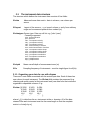
1.3. Estimation methods
Five different estimation methods can be used. Each has different levels of
performance in terms of accuracy, speed and suitability for different data types:
•
•
•
•
•
DFTM: Direct Fourier Transform Method (Barber 1961)
EMLM: Extended Maximum Likelihood Method (Isobe et al. 1984)
IMLM: Iterated Maximum Likelihood Method (Pawka 1983)
EMEP: Extended Maximum Entropy Method (Hashimoto et al. 1993)
BDM: Bayesian Direct Method (Hashimoto and Kobune 1987)
The code for the implementation the EMEP and BDM methods are based on
algorithms described by Hashimoto (1997). The IMLM method uses a modified
algorithm based on the one described by Pawka (1983).
Performance tests of the different methods have been carried out by Hashimoto
(1997) and Benoit (1993) for different measurement arrangements and spectral
shapes.
2. Installation
DIWASP is simply a collection of MATLAB m-file functions which carry out the
calculation of the directional spectrum and perform functions like plotting and
reading/writing data files. To make sure the functions work correctly:
1. Unzip or copy files to the same directory. This directory should be called
“diwasp”.
2. Supporting functions must remain in a subdirectory called private. If you
move the main functions you must move this subdirectory and its files to
the same location.
3. Add the new directory called “diwasp” with the main files
(dirspec,plotspec…etc..) to the MATLAB path. Do this using pathtool: see
MATLAB help for details.
The functions operate in the same way as any other MATLAB functions. Type
help [function name] for command-line help information. Type help diwasp at the
matlab prompt for help overview of the package.
3. DIWASP Data Structures
Data structures are used to manage input and output data compactly. A structure
is like a container and has a set of fields for each data types. Each field is
referenced using the ‘.’ operator between the structure name and the field name.
So Struct.A would references the data in field A of structure Struct. See the
MATLAB help regarding structures if you are unfamiliar with these ideas. The
advantage is that the entire data container can be passed as a single argument
to various functions
There are 3 main data structures used in DIWASP:
1. The instrument data.(ID) This contains the layout of the instrument
sensors, the type of sensors and the actual sensor data itself.
2. The spectral matrix.(SM) This is the output from the main calculation and
contains fields which define the bins of the output matrix, the orientation of
the axes system relative to true north and the spectral density itself.
3. The estimation parameters.(EP) This contains all the information
regarding how the directional spectrum estimation is actually carried out.
The variable names in brackets are used throughout to identify a structure of that
type. Note however that each of the structures can be given an arbitrary unique
name and then passed to the functions to carry out operations. As with any other
structures however, the field names must not be changed. Each of the three main
structures is discussed in more detail below.
3.1. The instrument data structure
The structure which defines the instrument data consists of five fields:
ID.data
Measured wave data matrix - data in columns, one column per
sensor
ID.layout
Layout of the sensors - x,y,z in each column. x and y from arbitrary
origin and z measured upwards from seabed (m)
ID.datatypes Sensor type. Enter as cell list: e.g. {'elev' 'pres'}
Currently supported:
'elev' surface elevation
'pres' pressure
'velx' x component velocity
'vely' y component velocity
'velz' z component velocity
'vels' vertical velocity of surface
'accs' vertical acceleration of surface
'slpx' x component surface slope
'slpy' y component surface slope
'accx' x component acceleration
'accy' y component acceleration
'accz' z component acceleration
'dspx' x displacement
'dspy' y displacement
ID.depth
Mean overall depth of measurement area (m)
ID.fs
Sampling frequency of instruments - must be single figure for all(Hz)
3.1.1. Organizing your data for use with dirspec
There are 3 main fields associated with the actual input data. Each of these has
one column for each instrument. The ID.data field contains the processed (e.g.
cleaning and quality control at the instrument level) raw data from the instrument
organized in sequential columns. E.g.:
ID.data= [0.3256
0.3345
0.3546
I1(t4)
….
0.3421
0.5643
0.7658
I2(t4)
…
0.4324
0.2345
0.1235
I3(t4)
…
];
where Im(tn) is data from the mth instrument at the nth timestep. All of the data
streams from each instrument must be the same length so that the complete
matrix is of size[n by m];
The ID.layout field contains the data about the instrument layout. As with the
ID.data field, each instrument has its own column with a row for x,y and z
position respectively (x and y relative to arbitrary origin, z height above seabed).
Continuing the example above, if the three instruments were pressure gauges
spread in a triangle on the sea floor the layout field might be:
ID.layout = [ 0.0
0.0
0.0
5.0
5.0
0.0
-5.0
5.0
0.0];
The instrument positions are [0,0] ,[5,5] and [-5,5] on a coordinate system with
the first sensor as the origin and the x axis defined to coincide with the x axis of
the instrument setup (directions are returned relative to these axes).
The datatype field describes the sensor type using one of the defined sensor
codes. These must be in single quotes and entered as a cell array using curly
brackets. For the example above, this would be:
ID.datatypes = {‘pres’ ‘pres’ ‘pres’};
As a second example, if a directional current meter and a pressure sensor were
all mounted on the same pod 0.5m above the seabed the layout and datatypes
fields would be:
ID.layout =
[ 0.0 0.0
0.0
0.0
0.0
0.0
0.5
0.5
0.5 ];
ID.datatypes = {‘velx’ ‘vely’ ‘pres’};
with ID.data placed in columns accordingly.
The sampling frequency, ID.fs must be the same for all of the sensors (data
columns) and each data stream is assumed to be synchronous (i.e. data point
no.254 is assumed to be from the same time for all instruments). The ID.depth
field is an average for the sampling area and is used in calculations involving the
linear dispersion relation1.
3.2. The spectral matrix structure
The spectral matrix structure has four fields:
SM.freqs
1
Vector of length nf defining bin centres of the spectral matrix
frequency axis
Note that no correction is carried out for the effect of a mean current even when the velocities
are given as part of the input data. Results may be significantly affected in the case of strong
mean currents. In these cases, the data must be pre-processed before use in DIWASP.
SM.dirs
Vector of length nd defining bin centres of the spectral matrix
direction axis
SM.S
Matrix of size [nf,nd] containing the spectral density
SM.xaxisdir The compass direction of the x axis from which angles are
measured.
SM.funit
Frequency units: can be ‘Hz’ or ‘rad/s’ [Default ‘Hz’]
SM.dunit
Directional units: [Default ‘cart’]
‘rad’ : Cartesian radians
‘cart’ : Cartesian degrees (original DIWASP units)
‘naut’ : Absolute nautical bearing waves coming from
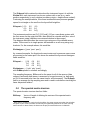
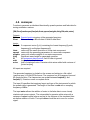
The layout of the spectral matrix is specified as a vector of evenly spaced
frequencies, SM.freqs and a vector of evenly spaced directions, SM.dirs. These
form the bin structure for the matrix and are the values are the centre of the bin
(Spectral matrix layout for components S). Frequencies (f) can be Hz or rad/s
(SM.funit) and directions (θ) are specified in degrees or radians measured
anticlockwise from the positive x axis. There is also the option of direction in
nautical convention – these are the direction the waves are coming from as a true
compass bearing.
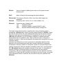
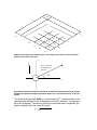
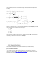
Internally, the orientation of a wave component is calculated relative to the x
direction of the instrument layout and wave recorder directional components
(Orientation of direction relative to coordinate system for instrument layout and
velocity components. With the compass orientation shown, the x axis direction is
90). SM.xaxisdir defines the compass direction of the x axis. In Orientation of
direction relative to coordinate system for instrument layout and velocity
components. With the compass orientation shown, the x axis direction is 90 this
would be 90o as with the axis orientation as shown by the north arrow. At the end
of the estimation function, directions are converted to the user specified units
SM.dunit.
Snf/nd
Dn
d
Fnf
Etc….
….
S32
.
S13
D4
S22
S12
D3
S31
F4
S21
S11
D2
…..
S41
F3
F2
F1
D1
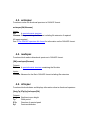
Spectral matrix layout for components Sij. The frequency bin vector is Fi(1:nf) and the
direction bin vector is Dj(1:nd).
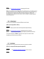
y
N
Wave component
travelling in this
direction
o
+30
x
Orientation of direction relative to coordinate system for instrument layout and velocity
components. With the compass orientation shown, the x axis direction is 90 o in the file
header.
The spectral density itself, SM.S is a matrix such that S ij contains values of the
spectral power density for the ith frequency and the jth direction. The energy is
per unit [Hz.degree]. Therefore to convert to component wave amplitudes you
need to multiply by the bin sizes df and dθ:
aij = 2 * S ij * df * dθ
where aij is the amplitude of the component with the ith frequency and the jth
direction and S ij is the value in the spectral density matrix. If you change
between Hz & rad/s or degrees & rads then you must also convert the energy
density value.
3.3. The estimation parameter structure
The structure which defines the estimation method and other parameters
consists of five fields:
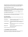
EP.method Estimation method used. Currently supported:
'DFTM'
'EMLM'
'IMLM'
'EMEP'
'BDM'
Direct Fourier transform method
Extended maximum likelihood method
Iterated maximum likelihood method
Extended maximum entropy principle
Bayesian direct method
EP.nfft
Number of DFTs used to calculate the frequency spectra: frequency
resolution is ID.fs / EP.nfft
EP.dres
Directional resolution of calculation itself specified as the number of
directional bins which cover the whole circle. Note that the actual
output resolution is determined by SM.dirs
EP.iter
Number of iterations: this has various effects for different methods
EP.smooth Smoothing applied: 'ON' or 'OFF'
If any fields default settings will be used for the others if not directly specified.
3.3.1. Estimation methods
A full discussion of the relative merits or disadvantages of each method are
beyond the scope of this manual. The papers by Hashimoto (1997) or Benoit
(1993) are good places to start looking for more information. A brief summary of
each method is given below:
•
•
DFTM Very fast method that is good for an initial overview of the spectral
shape. However directional resolution is poor and negative energy
distribution sometimes occurs. Poor tolerance of errors in the data.
EMLM Fast method that performs well with narrow unidirectional spectra.
Can provide extremely good accuracy per computation time in some
cases. Poor tolerance of errors in the data can lead to negative energy or
even failure of the method.
•
•
•
IMLM Refinement of the EMLM that iteratively improves the original EMLM
estimate. Highly dependent on the quality of the original solution so will
tend to perform poorly in the same situations as the EMLM. Will tend to
reduce anomalies such as negative energy in the EMLM solution.
Computation time directly dependent on number of refining iterations but
provides good accuracy for reasonable computing time. Can overestimate
peaks in the directional spectra by overcorrecting the original estimate.
EMEP Good all-round method that accounts for errors in the data.
Computation time is highly variable depending on how easily the iterative
computation finds the solution. This method can be as fast as the
IMLM(running with a default 100 iterations) and give far superior results. In
other cases it is significantly slower. Low spectral energies at low and high
frequencies can cause problems with the solution and slow the
computation. In these cases the computation may need to be successively
over-relaxed to achieve a converging solution. This is used as the default
method.
BDM Overall probably the best estimate but very computationally
intensive. Computational expense is highly dependent on the directional
resolution. As with the EMEP low energies can slow the computation due
to the need for progressively relaxing the computation to achieve
convergence. This method can also have problems with three quantity (i.e.
pressure + velocities or heave-roll-pitch from a single location)
measurements.
One recommended procedure for deciding which method to use is to use
testspec to test a given instrument array with a directional spreading similar to
what is expected from the data. This should give a good idea of the accuracy and
speed of operation of each method. However testspec does not simulate errors
which occur in real data.
Other tips (see options below for changing settings):
• All: Reduce the frequency resolution to increase computation speed
• EMEP/BDM: Reduce the directional resolution to increase computation
speed
• EMEP/BDM: There is usually an optimal number of iterations to allow
before the computation is relaxed. Too few and relaxation occurs when not
necessary, too many and a lot of iterations are performed in cases where
the computation does need to be relaxed..
• Use the EMEP or BDM method for data heavily contaminated with errors.
• If complete garbage comes out of the EMEP/BDM methods, do a check
with the DFTM method. This method is very unlikely to blow up so if this
does not produce something sensible, chances are the inputs are wrong.
3.3.2. Resolution of the estimation method
The fields EP.nfft and EP.dres control the resolution of the calculation and
hence the maximum resolution that can be achieved in the output spectral matrix.
EP.nfft is the number of DFTs carried out in the calculation of the cross-power
spectra. Higher numbers result in greater frequency resolution. This argument is
passed to the function diwasp_csd, which performs the same function as the
MATLAB function csd. The actual number of frequencies over which the
directional estimation is performed is bounded at the upper limit by the highest
value in the SM.freqs field. If EP.nfft is not explicitly specified a default value
based on the sampling frequency is used.
EP.dres is the number of directional bins used in the estimation calculation. The
computation is carried out for a complete circle of directions. The default setting
of 180 therefore gives a bin size of 2 degrees. The actual directions of the bins in
the output matrix are specified by SM.dirs and SM.dunit. Reducing this value
can dramatically improve computation speed for the EMEP and BDM methods.
EP.smooth is a simple on/off switch that determines if smoothing is applied to
the final spectra. This can be beneficial as it removes any spikes (which are in
any case not physically likely) and by default is on. The smoothing algorithm uses
a simple 5-point weighted average along both the frequency and directional axes.
3.3.3. Algorithm iterations
The IMLM, EMEP and BDM methods use an iterating algorithm. EP.iter sets the
number of iterations which has a slightly different effect in each method. The
exact effect is slightly different in each case. By default it is set to 100.
For the IMLM method this is the number of ‘improvement’ corrections carried out
at each frequency. It therefore directly affects the computation time but higher
numbers in theory give better results.
For the EMEP and BDM methods this value limits the number of iterations before
the computation algorithm ‘relaxes’ the iterative calculation. Reducing this
parameter does not necessarily lead to greater speed for these methods if the
algorithm is not reaching the iteration limit.
4. DIWASP functions
4.1. dirspec
Main directional estimation routine. Takes measured data and information about
sensors and returns the estimated directional spectrum.
[Smout,EPout]=dirspec(ID,SM,EP,{options})
Outputs:
SMout A spectral matrix structure containing the results
Epout
The estimation parameters structure with the values actually used for
the computation including any default settings.
Inputs:
ID
SM
EP
An instrument data structure containing the measured data
A spectral matrix structure; data in field SM.S is ignored.
The estimation parameters structure. To use all default values enter an
empty matrix:[ ].
{options} options entered as cell array with parameter/value pairs: e.g.
{‘MESSAGE’,1,’PLOTTYPE’,2};
Available options with default values:
'MESSAGE',1, Level of screen display: 0,1,2 (increasing output)
'PLOTTYPE',1, Plot type: 0 none, 1 3d surface, 2 polar type plot, 3 3d
surface(compass angles), 4 polar plot(compass angles)
'FILEOUT',''
Filename for output file: empty string means no file output
Input structures ID and SM are required. EP must be included but can be input as
an empty matrix if the default estimation parameters are required. {options} is an
optional input.
dirspec calculates the directional spectra using internally defined frequency and
directional bins.
The actual output is mapped onto the spectral matrix defined by SM.freqs and
SM.dirs. For more information on the spectral matrix see section 3.2. Choosing a
resolution that matches the resolution of the calculation is also important, as
excessively small bin sizes will result in a memory hungry output that does not
contain additional information. Also see the section 3.3.2 below for more
information on setting the resolution of the calculation.
The options input allows you to control the screen and file output. These must be
arranged in a cell array in parameter/value pairs as follows:
•
'MESSAGE' Default value=1
This sets the ‘noise level’ of screen display: 0 show minimal screen
information, only showing the main calculation steps. 1 shows more
information including the frequency being calculated and the model
number in the case of the EMEP and BDM methods. With this setting
(and 0) MATLAB warning messages are also suppressed. 2 outputs
all available information including warnings and state of relaxation.
Note that warnings regarding matrix solutions may be shown but the
algorithms should deal with these in most cases.
'PLOTTYPE' Default value=1
This sets the type of plot output shown at the end of the calculation.
Plot type 0 suppresses the plotting function, 1 - 4 are passed directly
to plotspec as parameter ptype.
'FILEOUT' Default value=’’
This option sets the filename for the output file containing the
calculated spectrum. This simply enables or disables a switch that
calls writespec with input arguments SM and the filename. An empty
string: ’’ means no file is output.
•
•
4.2. plotspec
Plotting routine for directional spectrum.
plotspec(SM,ptype)
Inputs:
SM
ptype
A spectral matrix structure
plot type:
1 3D surface plot
2 polar type plot
3 3D surface plot (compass bearing angles)
4 polar type plot (compass bearing angles)
The 3D surface plot type is a MATLAB surface plot with SM.freqs on the x axis,
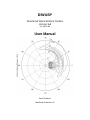
SM.dirs on the y axis and the spectral density, SM.S as the z value. The polar
type plot is a MATLAB polar plot with the direction showing values in SM.dirs,
the radius showing values in SM.freqs and contours representing the spectral
density, SM.S. An example of the polar type plot is shown on the front cover of
the manual.
For both plot types 1 and 2, the direction is the direction of propagation relative to
the Cartesian axis.
For options 3 and 4 the direction is coming from as a true compass bearing (this
has changed from previous versions).
Directions are corrected internally from the SM.xaxisdir and SM.dunit fields that
define the orientation of the axes and directional units in the spectral matrix.
4.3. writespec
Function to write out directional spectrum in DIWASP format.
writespec(SM,filename)
Inputs:
SM
A spectral matrix structure
filename String containing the filename including file extension if required
All inputs required
See 5.The DIWASP spectrum file format for information on the DIWASP format.
4.4. readspec
Function which reads in directional spectrum in DIWASP format.
[SM]=readspec(filename)
Outputs:
SM
A spectral matrix structure containing the file data
Inputs:
filename filename for the file in DIWASP format including file extension
4.5. infospec
Function which calculates and displays information about a directional spectrum
[Hsig,Tp,DTp,Dp]=infospec(SM)
Outputs:
Hsig
Tp
DTp
Dp
Signficant wave height
Peak period
Direction of spectral peak
Dominant direction
Inputs:
SM
A spectral matrix structure containing the file data
Hsig is the significant wave height. Tp is the peak frequency, the highest point in
the one dimensional spectrum. DTp is the main direction of the peak period (i.e
the highest point in the two-dimensional directional spectrum). Dp is the
dominant direction defined as the direction with the highest energy integrated
over all frequencies.
4.6. interpspec
Function which interpolates between different matrix bases
[SMout]=infospec(SMin, SMout)
Outputs:
SMout Output spectral matrix with interpolated spectral density
Inputs:
SMin
SMout
A spectral matrix structure containing the input spectrum
The spectral matrix specifying the frequency and directional axes.
The spectral density in SMout is ignored in the input, but needs to have
frequency and directional axes defined.
4.7. testspec
Testing function for directional wave spectrum estimation methods.
[EPout] = testspec(ID,theta,spread,weights,EP)
Outputs:
EPout
Inputs:
The estimation parameters structure used in the test.
ID
theta
spread
weights
EP
An instrument data structure containing the measured data. The
ID.data field is ignored.
vector with the mean directions of a sea state component
vector with the spreading parameters of a sea state component
vector with relative weights of sea state components
The estimation parameters structure with the values under test
used. Default settings are used where not specified.
All inputs are required
Testspec details:
The fields ID.layout and ID.datatypes and ID.depth are used to specify the
arrangement of the imaginary sensors.
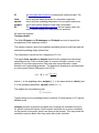
The function outputs a plot of the specified spreading function (solid line) and the
estimated spreading shape (dotted line).
The calculation is carried out for a frequency of 0.2 Hz.
The inputs theta, spread and weights determine the shape of the directional
spreading function. Each of these inputs is a vector of length n where n is the
number of sea state components. Each sea state component has a mean
direction and a spreading parameter. The directional spreading is calculated with
a cosine power function (Mitsuyasu et al.1975):
θ −θi 
G (θ ) = ∑ α i cos 2 Si 

 2 
i
where α i is the weighting value, weights(i), θ i is the mean direction, theta(i) and
Si is the spreading parameter, spread(i) where i=1…n.
The weights are normalized so that:
2
∫0
G d =1
Typical values for the spreading function would be 10 (wind waves) to 75 (narrow
banded swell).
testspec provides a powerful and quick way of testing the estimation functions
for specific instrument layouts. Note however that there are no errors simulated
so the pseudo cross power spectra are clean in that respect. This may cause the
methods to perform better than they would with similar real data.
4.8. makespec
Function to generate an idealized directionally spread spectrum and fake data for
testing estimation routines.
[SM,IDout]=makespec(freqlmh,theta,spread,weights,Hsig,SM,ndat,noise)
Outputs:
SM
Spectral matrix structure of the generated spectrum
IDout
Returns the input ID with data in field ID.data filled
Inputs:
freqlmh 3 component vector [l p h] containing the lowest frequency(l),peak,
frequency(p) and highest frequency(h)
theta
vector with the mean directions of a sea state component
spread vector with the spreading parameters of a sea state component
weights vector with relative weights of sea state components
Hsig
Significant wave height for generated spectrum
ID
An instrument data structure; field ID.data is ignored
ndat
length of simulated data
noise
level of simulated noise: Gaussian white noise added with variance of
[noise*var(eta)]
All inputs are required
The generated spectrum is plotted on the screen and written to a file called
‘specmat.spec’ in DIWASP file format. The spectrum has 50 frequency bins and
60 directional bins. The frequencies are spread between freqlmh(1) and
freqlmh(3). Directions cover a complete circle.
The input ID specifies the imaginary layout and type of the instruments for which
the pseudo data is generated. The length of the data is ndat with a sampling
frequency of ID.fs.
The input noise allows the addition of noise to the fake data to more closely
simulate real sensor outputs. The noise added is gaussian white noise with a
variance of noise*var(eta) where var(eta) is the variance of the simulated data
eta before addition of noise. The input noise should be set to zero for a clean
signal.
The simulated spectrum is constructed using a TMA spectral shape (Bouws et
al.1985):
ETMA ( f ) = E k ( f ).φ PM ( f / f m )φ J ( f , f m , γ , σ a , σ b )
φ PM
−4

 f  
= exp − 5 / 4  

 f m  
σ

f m ≥ f 
 − ( f − f m ) 2 
 a


φ J = exp ln ( γ ) exp

2 2
 σ = 
fm < f 

σ b
 2σ f m 

0.5ω 2
ω H ≤ 1
H




−4
2
−5
E k = α .g ( 2π ) f φ K φ K =  1
1 < ω H < 2  ω H = 2π . f H / g


2
ωH ≥ 2 
 1 − 0.5 2 − ω

(
)
(
)
where H is the depth and f m is the dominant frequency, input freqlmh(2) and the
other parameters are constants set internally to:
α = 0.014
γ =2
σ a = 0.07
σ b = 0.09
The spectrum is scaled so that it has Hrms equal to the input Ho. The directional
spreading is calculated as described in testspec.
4.9. Internal functions
The functions contained in the private subdirectory are used internally.
4.9.1. Transfer functions
The transfer functions map a surface elevation to an equivalent instrument
response for a given depth. The transfer functions have the same name as the
datatypes described in The instrument data structure.
New transfer functions or estimation methods can be incorporated by simply
including a new transfer function m-file and then using calling the filename as a
new datatype argument. New transfer functions must operate as follows:
[trm]=newf (ffreqs,ddirs,wns,z,depth)
ffreqs is a column vector of size [nf,1] and ddirs is a row vector of size [1,nd]
containing the frequency and direction bins of the calculation (as distinct from the
spectral matrix bins). wns is a vector the same size as ffreqs of wavenumbers
corresponding to the frequencies.
z is the height of the instrument sensor above the bed and depth is the total
mean depth of the instrument location.
trm must be returned as a size[nf,nd] matrix with the [i,j] element corresponding
to the transfer function for the ith frequency and the jth direction.
4.9.2. Other functions
Some of the private functions may be useful as stand alone functions for other
applications. These include:
wavenumber.m
Calculates wavenumbers for given frequency and depth
from linear wave dispersion relation.
makerandomsea.m
Creates a random surface elevation for a given spectrum
of component amplitudes. Useful for visualising sea
states.
makewavedata.m
Make random sea elevation data for a specified spectrum
and layout of probes.
diwasp_csd.m
Replacement function for Matlab csd/cpsd that only
requires inbuilt fft function.
Usage is described in the command line help
5. The DIWASP spectrum file format
DIWASP uses its own format for storing the spectrum files. It is intended to be
simple and easy to incorporate into other software on any platform.
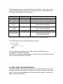
The file format consists of a single ASCII stream of numbers. The header section
contains information about the layout of the spectral matrix, and the body of the
file contains the energy of each component.
Position in file
1
2
3
4..
nf+3
nf+4..
nf+nd+3
Type(FORTRAN)
Real
Integer
Integer
Real
nf+nd+4
nf+nd+5..
nf+nd+(nf*nd)+4
Integer
Real
Real
Compass direction of x axis
Number of frequency bins (nf)
Number of directional bins (nd)
List of frequencies starting with low values
This is the vector SM.freqs
List of directions starting with low values
This is the vector SM.dirs
Value:999 Marks end of the header
Spectral density for each bin with frequency
as the outside of the loop*
This is the matrix SM.S
*All the directions are given for the first frequency then all for the second frequency etc.
The FORTRAN code for reading the spectral density is:
do i=1,nspec
do j=1,ndir
read(##,*) S(i,j)
enddo
enddo
A Fortran subroutine readspec.f with code to read the DIWASP format is
provided with the DIWASP package.
The functions readspec.m and writespec.m read and write from DIWASP spectral
matrix structures to DIWASP file format.
6. Code, bugs and modifications
DIWASP is written to be functional and easy to use. Although there is some error
checking, this really only verifies the shapes of the inputs, not whether they make
sense. If you are getting garbage out of dirspec check your inputs - chances are
they are somehow incorrect.
The code has not been fully streamlined to keep the program structure clear and
user modification of code should be relatively easy. This does mean however that
the functions do not run as fast as they might, although recent versions of MAtlab
have improved execution speeds. If you want high-end performance some
modification will help or rewrite code in Fortran or similar.
Updated versions of DIWASP will be made available as and when they are
produced. I am grateful for the bug reports and suggestions I have received to
date. If you find bugs in the code, have any suggestions for modifications or,
more seriously, find errors in the actual algorithms, please contact the author:
Email: [email protected]
David Johnson
Metocean Solutions Ltd. (www.metocean.co.nz)
New Zealand
This version of DIWASP is freeware and doesn’t come with any kind of official
support. It is intended for the benefit of the coastal and ocean science
community. Hopefully it might save you some time in analysing your wave data.
Good luck and enjoy.
7. References
Barber,N.F. (1961) The directional resolving power of an array of wave detectors,
Ocean Wave Spectra. Prentice Hall. Inc. pp.137-150
Benoit,M. (1993) Practical comparative performance survey of methods used for
estimating directional wave spectra from heave-pitch-roll data. Proc.23rd ICCE
Vol 1. ASCE pp.62-75
Bouws,E., Gunther,H., Rosenthal,W. and Vincent,C.L. (1985) Similarity of the
wind wave spectrum in finite depth water. 1.Spectral form. J.Geophys.Res.
90(C1) 975-985
Hashimoto,N. (1997) Analysis of the directional wave spectra from field data.
Advances in Coastal and Ocean Engineering Vol.3. ed.Liu,P.L-F. World
Scientific, Singapore. pp.103-143
Hashimoto,N. and Kobune,K. (1988) Estimation of directional spectrum from a
Bayesian approach. Proc.21st ICCE Vol 1. ASCE pp.62-72
Hashimoto,N. Nagai,T and Asai,T. (1993) Modification of the extended maximum
entropy principle for estimating directional spectrum in incident and reflected
wave field. Rept. Of P.H.R.I. 32(4) 25-47
Isobe,M., Kondo,K. and Horikawa,K. (1984) Extension of MLM for estimating
directional wave spectrum. Proc. Symp. on Description and Modeling of
Directional Seas, Paper No.A-6. 15pp.
Mitsuyasu,H. et al.(1975) Observation of the directional spectrum of ocean wave
using a cloverleaf buoy. J.Phys.Oceanogr. 5 750-760
Pawka,S.S.(1983) Island shadows in wave directional spectra. J.Geophys.Res.
88(C4) 2579-2591