Download funwaveC Users Manual

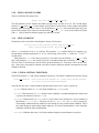
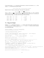
funwaveC Users Manual
Falk Feddersen
July 31, 2007
Contents
1 Introduction
3
2 Compiling
2.1 Required Libraries . . . . . . . . . . . . . . . . . . . . . . . . . . . . . . . . . . . . . . .
2.2 Unpacking, configure, and make . . . . . . . . . . . . . . . . . . . . . . . . . . . . . . . .
2.2.1 Apple Mac G4 Hack . . . . . . . . . . . . . . . . . . . . . . . . . . . . . . . . . .
4
4
4
5
3 Running funwaveC
3.1 Invoking funwaveC . . . . . . . . . . . . . . . . . . . . .
3.2 Init File . . . . . . . . . . . . . . . . . . . . . . . . . . .
3.2.1 Example Init File . . . . . . . . . . . . . . . . . .
3.3 Init File Input Stuff . . . . . . . . . . . . . . . . . . . . .
3.3.1 LINE 1: MODEL DYNAMICS . . . . . . . . . .
3.3.2 LINE 2: GRID SIZE & SPACING . . . . . . . . .
3.3.3 LINE 3: BOTTOM STRESS INFORMATION . .
3.3.4 LINE 4: LATERAL FRICTION INFORMATION
3.3.5 LINE 5: BATHYMETRY . . . . . . . . . . . . .
3.3.6 LINE 6: WAVEMAKER . . . . . . . . . . . . . .
3.3.7 LINE 7: BREAKING . . . . . . . . . . . . . . .
3.3.8 LINE 8: SPONGE LAYERS . . . . . . . . . . . .
3.3.9 LINE 9: FORCING . . . . . . . . . . . . . . . .
3.3.10 LINE 10: INITIAL CONDITIONS . . . . . . . .
3.3.11 LINE 11: TRACER . . . . . . . . . . . . . . . .
3.3.12 LINE 12: FLOATS . . . . . . . . . . . . . . . . .
3.3.13 MODEL TIMING . . . . . . . . . . . . . . . . .
3.3.14 OUTPUT . . . . . . . . . . . . . . . . . . . . . .
3.4 Diagnostic Output . . . . . . . . . . . . . . . . . . . . . .
3.4.1 General funwaveC information . . . . . . . . . .
3.4.2 Timing Report . . . . . . . . . . . . . . . . . . .
3.5 Model Stability . . . . . . . . . . . . . . . . . . . . . . .
3.5.1 CFL Stability Criteria . . . . . . . . . . . . . . .
3.5.2 Sponge Layer Stability Criterion . . . . . . . . . .
3.5.3 Biharmonic Friction and Stability . . . . . . . . .
1
.
.
.
.
.
.
.
.
.
.
.
.
.
.
.
.
.
.
.
.
.
.
.
.
.
.
.
.
.
.
.
.
.
.
.
.
.
.
.
.
.
.
.
.
.
.
.
.
.
.
.
.
.
.
.
.
.
.
.
.
.
.
.
.
.
.
.
.
.
.
.
.
.
.
.
.
.
.
.
.
.
.
.
.
.
.
.
.
.
.
.
.
.
.
.
.
.
.
.
.
.
.
.
.
.
.
.
.
.
.
.
.
.
.
.
.
.
.
.
.
.
.
.
.
.
.
.
.
.
.
.
.
.
.
.
.
.
.
.
.
.
.
.
.
.
.
.
.
.
.
.
.
.
.
.
.
.
.
.
.
.
.
.
.
.
.
.
.
.
.
.
.
.
.
.
.
.
.
.
.
.
.
.
.
.
.
.
.
.
.
.
.
.
.
.
.
.
.
.
.
.
.
.
.
.
.
.
.
.
.
.
.
.
.
.
.
.
.
.
.
.
.
.
.
.
.
.
.
.
.
.
.
.
.
.
.
.
.
.
.
.
.
.
.
.
.
.
.
.
.
.
.
.
.
.
.
.
.
.
.
.
.
.
.
.
.
.
.
.
.
.
.
.
.
.
.
.
.
.
.
.
.
.
.
.
.
.
.
.
.
.
.
.
.
.
.
.
.
.
.
.
.
.
.
.
.
.
.
.
.
.
.
.
.
.
.
.
.
.
.
.
.
.
.
.
.
.
.
.
.
.
.
.
.
.
.
.
.
.
.
.
.
.
.
.
.
.
.
.
.
.
.
.
.
.
.
.
.
.
.
.
.
.
.
.
.
.
.
.
.
.
.
.
.
.
.
.
.
.
.
.
.
.
.
.
.
.
.
.
.
.
.
.
.
.
.
.
.
.
.
.
.
.
.
.
.
.
.
.
.
.
.
.
.
.
.
.
.
.
.
.
.
.
.
.
.
.
.
.
.
.
.
.
.
.
.
.
.
.
.
.
.
.
.
.
.
.
.
.
.
6
6
6
6
8
8
8
8
8
9
9
11
12
12
12
13
13
13
14
16
17
17
17
17
18
18
4 Model Equations and Numerics
19
4.1 The Surfzone Circulation Model . . . . . . . . . . . . . . . . . . . . . . . . . . . . . . . . 19
4.2 The Staggered C-Grid and discretization . . . . . . . . . . . . . . . . . . . . . . . . . . . . 20
4.3 Model time-stepping . . . . . . . . . . . . . . . . . . . . . . . . . . . . . . . . . . . . . . 21
5 File Structure Overview
22
6 Tests and Example .init Files
23
7 MATLAB scripts for setup and processing
24
8 Bugs
25
2
Chapter 1
Introduction
funwaveC is an implementation in the C programming language of the fully nonlinear boussinesq equations
of (Wei et al., 1995) that also includes the extensions for a wave generation and wave breaking. funwaveC is
essentially a re-implementation of the FUNWAVE model (e.g., Chen et al., 1999; Kennedy et al., 2000)
from the University of Delaware (http://chinacat.udel.edu/...). For my own research projects, I needed
to use a Boussinesq wave model, and the reason why I undertook this re-implementation is essentially
because FUNWAVE is written in FORTRAN (FORTRAN77 no less!). As a former computer scientist I
cannot abide FORTRAN. For those who do not appreciate the differences in programming langagues and
the practices they enforce, this may seem trivial. However, it makes a world of difference in creating clean,
debuggable, and maintainable code. So I decided to begin with an existing nonlinear shallow water equation
code I had previously developed (used in Noyes et al., 2005) and develop it into a Boussinesq model. After
considering using C++, I choose to write the code in C because I was more familiar with it, it allowed me
to code both at high and low levels, and it is highly portable. In the end there are a number of differences
between funwaveC and FUNWAVE particularly in the numerics. However they have essentially the same
functionality and to show my respects, I choose to name the model funwaveC .
The model has been used now in studies of surfzone tracer (Feddersen, 2007) and drifter (Spydell and
Feddersen, 2007) dispersion and is currently being used in other projects as well. I felt it would be useful
to others to release it publically under the GNU Public License Version 2 (http://gnu.org). The model has
been run in a variety of *NIX environments and in principle should compile and work on Windows as well
(with the Cygwin environment). Please note that funwaveC is a work in progress as is this user’s manual.
Neither are complete yet the model is certainly quite useful.
Please let me know if your experience with this model either fills you with joy or makes you cry! If you
have any problems or questions, do not hesitate to ask ([email protected])
3
Chapter 2
Compiling
2.1 Required Libraries
To compile the program, one must first have certain libraries installed on the system. In particular, the
glib and gtk libraries must be present with a 1.2 series version number. The glib library is used to handle
various I/O and memory resource things. The gtk libarary handles all the GUI window stuff. These libraries
work together and are installed on most GNU/Linux and UNIX systems. They can be installed on OS X
using fink. The source code for the libraries also can be downloaded from www.gtk.org and again both
rpms and source tar balls are available. If you use rpms make sure the appropriate header files are installed.
This may require also installing the development version of glib.
Installation of glib and gtk can be checked by typing at a shell prompt:
% glib-config --version
and
% gtk-config --version
If you get a response such as 1.2.8 then you are in business. I recommend using version > 1.2.8. Note the
2.0 series of these libraries will not work!
2.2 Unpacking, configure, and make
Once these libraries are installed, To build the program, untar the distribution funwaveC-0.2.0 directory.
Type the command
% ./configure
and then
make
The program should compile automatically. This has been configured for Linux, Sun, and OS X.
One can do a basic test of the newly compiled funwaveC by entering the tests directory and typing
make. This has funwaveC read in all the .init files in the tests directory, parse them, and quit. It does
not actually do any simulations. For more information on .init files see the next Chapter. For more
information on the test init files see the Tests Chapter.
4
2.2.1 Apple Mac G4 Hack
Note, there is a hack for compiling on Apple Mac G4 sytems with OS X. After running configure, you
need to open the file Makefile in an editor and add the following to the CFLAGS line: -mcpu=7450 which
tells the compiler to build for a G4 chip not a G5 chip. For example, replace:
CFLAGS = -fast ‘gtk-config --cflags‘
with CFLAGS = -fast -mcpu=7450 ‘gtk-config --cflags‘
I need to figure out how to set this in the configure process.
5
Chapter 3
Running funwaveC
3.1 Invoking funwaveC
funwaveC is run on the command line by invoking at the prompt:
% funwaveC test.init
where test.init is the name of the input file. There are a number of command line options that are
available. These are
-h Print out help information on usage and quit
-p Parse the input file to check for errors and quit
-g Opens up a GUI timing window while the model runs
-v Prints out model kinetic and potential energy at each level 1 time
-d [1,2,3] Prints out diagnostic information at either a level 1,2, or 3 time step
The verbose option tells the model to write out the value of the integrated kinetic and potential energy
at the end of every level1 time (defined later in model timing). This is useful for making sure that the model
isn’t going unstable. The diagnostic option (-d) takes an argument of 1,2, or 3 and reports on the hardwired options, the estimated memory usage, the stability parameters, the wavemaker, sponge layers, timing
info, and performs some basic tests (checking total water depth and testing continuity) at the beginning of
the model run and at the end of the intended timing level given by the argument. Thus -d 3 only gives
diagnostic output at the end of the model run. -d 1 gives diagnostic output at the end of every level1
iteration loop which is useful for diagnosing stability stuff.
3.2 Init File
funwaveC reads in a init file given on the command line. Customarily, this file is given the extension
.init, but this is not required. The init file details how the model is to be configured, from model type,
domain size, the wavemaker properties, to the output that is requested. In the tests directory, there are
many examples of init files for many different situations. Please see the Chapter on Tests.
3.2.1 Example Init File
The input information is given by the init filename on the command line. Comments are allowed in the
initfile by putting a ’%’ at the start of the comment line. A very basic init file example is:
funwaveC dynamics nwogu
6
dimension 11 10 1 1
bottomstress
0.01
mixing biharmonic0 1
bathymetry flat 1.0
eta_source off
breaking off
sponge
off
forcing none 0.0000 const 0.0001
initial_condition none 0 none 0 none 0
tracer off
floats off
timing 80 (min) 5 (min) 10 (sec) 0.01 (sec)
level1 cross U 0 file ascii Ucross.dat
level1 cross V 0 file ascii Vcross.dat
level1
cross N 0 file ascii eta_cross.dat
which used Nwogu Boussinesq wave dynamics (line 1), sets up a 11 by 10 grid with 1 m grid spacing
(line 2). The bathymetry is flat with depth of 1 m (line 5), and there is no wave generation (line 6), wave
breaking (line 7), or sponge layers (line 8) active in the run. There is an alongshore (y) forcing (e.g., due
to a wind stress) of 0.0001 m/s2 (line 9) and a drag coefficient (line 3) of cd = 0.01. The initial condition
(line 10) for u, v, and η are zero. Tracers (line 11) and floats (line 12) are not included in this run. The
model is to run for 80 minutes in 3 nested loops of 10 sec, 5 min, and finally 80 min (line 13). The time step
dt = 0.01 sec (line 13). Lines 14-16 describe the output that the model is to write. There is a wide variety
of possible model outputs. Here, the init file tells the model to output the cross-shore array at alongshore
location 0 of u, v, and η as ascii files with the given file names.
This example just gives a very small indication of the possibilities of the init file. The full form of the
init file, not including output (we’ll come to that later) is (quantities in [] denote the various options)
funwaveC dynamics [linear,peregrine,nwogu,wei_kirby]
dimension nx ny dx dy
bottomstress
c_d
mixing [none,newtonian0,biharmonic0] nu
bathymetry [flat,planar,file1d,file2d] ...
flat => bathymetry flat depth
planar => bathymetry planar depth0 slope
file1d => bathymetry file1d filename
file2d => bathymetry file2d filename
eta_source [on,off] [monochromatic,random1nb,random1file,random2nb,random2filea,random2fil
monochromatic => eta_source on monochromatic H
f theta i_wavemaker [delta]
random1nb
=> eta_source on random1nb
Hsig fp fwidth fnum theta i_wavemaker [delta]
random1file
=> eta_source on random1file spectra_file i_wavemaker [delta]
random2nb
=> eta_source on random2nb Hsig fp fwidth fnum theta spread i_wavemaker [
random2filea => eta_source on random2filea spectra_file i_wavemaker [delta]
random2fileb => eta_source on random2fileb spectra_file i_wavemaker [delta]
breaking [on,off] [zelt, kennedy,falk] [smooth,nosmooth] ....
zelt => breaking on zelt [smooth,nosmooth] [delta_b cI]
kennedy => breaking on kennedy [smooth,nosmooth] [delta_b cI cF Tstar ] defaults= [1.
falk => breaking on falk [smooth,nosmooth] [delta_b cI]
sponge
forcing
[on,off] num_x0 num_xL c_sponge
[none,const,file1d,file2d] (Fx,filename)
7
[none,const,file1d,file2d] (Fy,filename
initial_conditon [none,file1d,file2d] U_value [none,const,file1d,file2d] V_value [none,cons
tracer [on,off] [pointsource,alonglinesource] ix iy qsrc kappa start_time end_time
floats [on,off] [random,file,point] ...
random => floats on random N (N = number of floats)
filefloats => floats on file filename
timing level3_time (units) level2_time (units) level1_time (units) dt (units)
level3_time = total run time, level2_time = loop2 run time
level1_time = loop1 run time, dt = time step
units = [hr,min,sec]
Note that this information is given by the model with the help flag (-h). These quantities are now
described one by one.
3.3 Init File Input Stuff
3.3.1 LINE 1: MODEL DYNAMICS
The model dynamics are given by the first line of the init file which should look like
funwaveC dynamics [wei kirby,nwogu,peregrine,nswe,linear]
where the options in [] define chosen the model dynamics.
3.3.2 LINE 2: GRID SIZE & SPACING
The grid sizes are given by the first line of the init file as
dimension <nx> <ny> <dx> <dy>
Note that ny must be ≥ 6. The units of dx and dy are meters. For a run with a x and y domains of 1000 m
by 450 m and 5 meter grid spacing the line would read the line would be:
dimension 201 90 5 5
3.3.3 LINE 3: BOTTOM STRESS INFORMATION
bottomstress cd
The drag coefficient cd is nondimensional and is typically O(10−3 ). What this does is add a quadratic
bottom stress term of
−cd |u|(u, v)/d
(where d is the instantaneous depth) to the momentum equations.
3.3.4 LINE 4: LATERAL FRICTION INFORMATION
mixing [none,newtonian0,biharmonic0] nu
The lateral friction can be either none, newtonian0 or biharmonic0. nu is the lateral viscoscity or
hyperviscosity depending on the lateral friction chosen. What this does is adds a term to the right-hand-side
of the momentum equation a term either (for u)
+ν∇2 u,
−ν∇4 u
for newtonian or biharmonic fruction respectively.
8
Choosing the hyperviscosity for biharmonic friction:
monic friction... More later.
There are subtelties to choosing the ν for bihar-
3.3.5 LINE 5: BATHYMETRY
The fifth line loads the bathymetry. The format is
bathymetry [flat, planar, file1d, file2d] [h0, (slope h0), filename, filename]
The options for each are where <format> is either flat, planar, file1d, or file2d.
• flat: If flat, the bathymetry is assumed constant everywhere and is given (in meters) by h0.
• planar: When the format is:
bathymetry planar slope h0 the bathymetry is planar with constant slope in x that is given by
slope and depth at x = 0 of h0 (in meters).
• file1d: If the format is bathymetry file1d filename The alongshore uniform bathymetry if
loaded from the file filename which is an ascii file of a single vector of length nx-1. does not allow
for alongshore inhomogeneous bathymetry.
• file2d: If the format is
bathymetry file2d filename
the 2D bathymetry i sloaded up from the file filename which is an ascii file and a two-d array of
length [nx-1,ny].
3.3.6 LINE 6: WAVEMAKER
The 6th line sets the wavemaker stuff, which can be complicated. The line begins with,
eta source [on,off] [monochromatic, random1..., random2...]
...
The 2nd option sets the wavemaker to be on or off. If set to off then the rest of the line is ignored.
Monochromatic There are three essential type of wave options, monochromatic which is single frequency and single direction waves, essentially the spectrum is a delta function in frquency and direction,
i.e., E(f, θ) = E0 δ(f − f0 )δ(θ − θ0 ).
eta source on monochromatic H f theta i wavemaker [delta]
where H is the wave height in meters, f is the frequency in Hz, theta is the wave angle in degrees,
i wavemaker is the grid location in x where the wavemaker is centered. There is an optional parameter delta regarding the relative width of the wavemaker region. delta defaults to zero. See the funwave
manual for more info.
9
Random1 There is an option for narrow-banded random waves called random1nb. This parameter looks
like
eta source on random1nb Hsig fp fwidth fnum theta i wavemaker [delta]
Many of these options are similar to monochromatic. There is now the addition of fwidth - the width of
the spectral peak in Hz, and fnum - the integer number of discrete frequencies that make up the peak. This
should be odd.
The random1file option is for waves random in frequency but each frequency can have it’s own
direction, so that E(f, θ) = E(f )δ(θ − θ0 (f )). The form is
eta source on random1file spectra file i wavemaker [delta]
where the spectra file has 3 columns
f (Hz) a(f) (m), theta (deg)
where a(f) is the fourier amplitude at that frequency (not the spectra!).
Random2: There are three options for random directionally spread waves (random2). The first random2nb
is narrow-banded in frequency and direction and is similar to the random1nb option above:
eta source on random1nb Hsig fp fwidth fnum theta spread i wavemaker [delta]
where spread is the directional spread in degrees.
The second options random2filea is similar to random1file in that a directional spread is specified
at each frequency The form is
eta source on random2filea spectra file i wavemaker [delta]
where the spectra file has 4 columns
f (Hz) a(f) (m), theta (deg) spread (deg)
where a(f) is the fourier amplitude at that frequency (not the spectra!). This is only tested at a rudimentary
level...
The third option (random2fileb) specifies the full frequency-directional sprectra. The form of this is
similar,
eta source on random2fileb spectra file i wavemaker [delta]
but the spectra file now is different it looks like rows of θ and columns of frequency f ,
−1 θ1
θ2 ...
f1 a11 a12 ...
f2 a21 a22 ...
where aij are the fourier amplitudes at each frequency and direction.
Potential Bug: There may be problems in my conversion from θ to ky of the directional spectra. In a
continum
Z
Z
D(θ)dθ = 1 = D(ky )dky / cos(sin−1 ky )
could i be messing this up?
10
3.3.7 LINE 7: BREAKING
The 7th line sets the wave-breaking parameters. Breaking is simulated by using a eddy viscosity on the front
face of sufficiently steep waves. Breaking parameters are specified by:
breaking [on,off] [zelt,kennedy] [smooth,nosmooth] ....
If breaking is set to be off then the eddy viscosity always zero. If breaking is on then there are two types of
breaking options, zelt (Zelt, 1991) and the more complicated kennedy (Kennedy et al., 2000) breaking.
In addition, one must also specify whether a smoothed or a non-smoothed eddy viscosity is desired. The
eddy viscosity is smoothed on a 3 by 3 grid.
Zelt (1991)
breaking on zelt [smooth,nosmooth] [delta b cI ]
where the defaults are [1.2 0.3].
Kennedy et al. (2000)
breaking on kennedy [smooth,nosmooth] [delta b cI cF cT]
c where the 4 parameters control breaking. If not all the parameters are given then the defaults of [ 1.2
0.65 0.15 5 ] are used.
Falk breaking
breaking on falk [smooth,nosmooth] [delta b cI ]
where the defaults are [1.2 0.3]. This is NOT YET TESTED. USE AT YOUR OWN RISK!
Breaking Eddy Viscosity Definition
The breaking eddy viscosity is defined as
νbr = δb2 B(t)(h + η)ηt
(3.1)
where δb and B are non-dimensional. The parameters δb sets the overall magnitude of the eddy viscosity.
The parameter B is defined so that

 1, ηt > 2ηt∗
(3.2)
ηt /ηt∗ − 1, ηt > ηt∗
B=

0, ηt < ηt∗
Where ηt∗ is the critical free-surface elevation time-derivative which turns on wave-breaking. This is defined
as....
The falk breaking method is slightly different. If at any point B (as Zelt) becomes non-zero, then it
stays non-zero further offshore until ηt < 0. This is intended to better mimic the fact that white water of
breaking waves always stretches up until the top of the wave. We need to see how this works.
11
3.3.8 LINE 8: SPONGE LAYERS
The next line defines the sponge layer:
sponge [on,off] num x0 num xL c sponge
The 2nd parameter sets the onshore and offshore sponge layers as either on or off. The 3rd and 4th parameters (num x0 and num xL) set the number of grid points (U grid points?) on the onshore and offshore
boundary where the spong layer is active. The 5th parameter (c sponge) is the maximum linear drag coefficient for the sponge layer. Experience has shown that c sponge * dt < 0.25 for the model to be stable.
If the -d X flag is turned on then the sponge layer stability is tested.
3.3.9 LINE 9: FORCING
The nth line sets the cross-shore and alongshore forcing. The format is
forcing [none,const,file1d,file2d] (Fx,forcing file)
[none,const,file1d,file2d] (Fy,forcing file)
where none means there is no (x or y) forcing. The parameter const implies that there is constant x or y
forcing and the subsequent parameter (Fx or Fy) is the forcing value in units...?? (either ms−2 or m2 s−2 need to check).
With parameter file1d, the forcing is given by a cross-shore array in filename forcing file. Similarly, with parameter file2d, the forcing is given by a two-dimensional array in filename forcing file.
The size of the 1D and 2D arrays must be correct given the domain size. If not there will be an error message. Along rows correspond to constant cross-shore location, and down columns correspond to the same
alongshore location.
3.3.10 LINE 10: INITIAL CONDITIONS
The next line load the u, v, and η initial conditions respectively. The format is identical to that for the forcing
initial condition [none,const,file1d,file2d] Uic [none,const,file1d,file2d]
Vic [none,const,file1d,file2d] ETAic
where the first pair is the u initial condition and subsequent pairs are for v and η, respectively.
• none: With the choice of none, the initial condition for u, v, or η is zero.
• const: With the choice of const then the initial condition is constant throughout the domain and
is given by the numerical value in Uic, etc.
• file1d: With the choice of file1d the ic is a cross-shore array (uniform in y) of ascii numbers in
the filename Uic, Vic, ETAic. The array sizes are NX, NX+1, NX-1 for u, v, and η, respectively.
The boundary conditions that the model uses must already be set up in these initial conditions. This is
also rather kludgy but makes things simpler right now. If you don’t understand the u and v boundary
conditions consult the other documentation.
• file2d: With this choice the a 2-D initial condition field given in the filename is specified.
12
3.3.11 LINE 11: TRACER
tracer [on,off] [pointsource, alonglinesource] <ix> <iy> <qsrc> <kappa> <half life>
<start time> <end time>
where <qsrc> is the flux source in units ..., <kappa> is the lateral diffusivity in MKS, and <half life>
is the tracer half life in seconds. <start time> (in sec) indicates when the tracer release is to begin and
<end time> when it is to end. If these two parameters are missing then tracer release is assumed to begin
at the start of the run and continue until the end.
3.3.12 LINE 12: FLOATS
The next line controls the floats or drifters used in the model. The line format is,
floats [on,off] [random,file,point] ...
where the options are random positioning or positions input from a file.
Random Float Positioning:
For random float positioning choose
floats on random N (time)
where N is the number of floats. Optionally you can also specify a float release time (implemented yet?)
Floats Position Input File:
floats on file filename
where filename is the float input file. It has a format of columns of
x y (release time (recovery time))
where x and y are the release locations in meters and there is an optional release time and recovery time
(in seconds). If the release time is not given then it is assumed to be at the intial time (t = 0), and the
drifters are never recovered. If the release time is given but without a recovery time, then the drifters
are never recovered. Obviously there can be no recovery without a specific release time.
Point Drifter Release:
Still need to implement this.
3.3.13 MODEL TIMING
The 13th line, controls the timing of the program including total run time and the time step dt. Before
explaining the format, let me explain a little about how funwaveC runs. The heart of the integration code
takes place within three for loops which look like
for (i=0 to .... [loop3] )
for (j=0 to .... [loop2])
for (k=0 to .... [loop1])
time_step_model();
time=time+dt
13
The user has control of how much run time is spent within each loop. This is convenient when one wants
to specify the output that the model is to write. Output is covered in the next section. The timing control
line contains eight pieces, which must all be present. The format is
timing <total time> (<units>) <loop2 time> (<units>) <loop1 time> (<units>) <dt>
(<units>) The four times can be floating point numbers and their meanings are summarized below
• total time is the total time the model is to integrate for in the specified units.
• loop2 time is the time spent in loop2 (i.e. for (j=0 ...
• loop1 time is the time spent in loop1 (i.e. for (k=0 ...
• dt is the time step size of the model.
The are four possible choices for the units: (day), (hr), (min), (sec). Different times can have
different units.
Because the four different times control the number of iterations in the three loops (above), the four run
times must be integer divisible, that is,
total time/loop2 time
loop2 time/loop1 time
loop1 time/dt
must all be perfect integers (in common units of course). If not the model returns with an error message.
Note also that loop2 time can equal loop1 time and total time can equal loop2 time. This means
that one iteration of a loop occurs.
Here is an example of a timing line. Suppose one wants to run the model for a total of 24 hours, with
time step of 10 sec, and loop1 time of 30 min and loop2 time of 2 hours (note these values are all integer
divisible), then the timing line in the init file would look like:
1 (day) 2 (hr) 30 (min) 10 (sec)
3.3.14 OUTPUT
There are a number of functions which output the model data and are contained in the file output.h. There
are three options for output, (1) at the end of loop 1 - called level 1 output, (2) at the end of loop 2 - called
level 2 output, or (3) at the end of the model run - called level 3 output. This allows for a wide range of
output options at various time intervals. The line format in the init file is the same for all three cases and
looks like
<level[123]> arg1 arg2 arg3 arg4 arg5
where <level[123]> is the string “level1”, “level2”, or “level3”. There can be as many output commands
of this sort as desired (provisionally). Following we describe the detail of each level command.
There are six different output types for any level[123] output: (1) point, (2) along - alongshore
line, (3) cross - cross-shore line, (4) snapshot (2D map), (5) avgsnapshot, and (6) floats - documented later. Any of u, v, eta, vorticity (vort), breaking eddy viscosity (eddy), tracer, and cross-shore
(taubx) & alongshore (tauby) bottom stresses can be chosen as output variables for most output types.
Note that output parameters (except for filenames) are not case-sensitive. This means that eddy and EDDY
are treated the same.
14
Point Output: Point output is restricted to only variables u, v, eta, and tracer. This can be changed if
needed and is a relic of older code. For point output the format is:
level1 point [U,V,P,T] x-loc y-loc [file,term] [ascii,binary] filename
The parameters x-loc and y-loc are the index locations for the point output. The last two options
[ascii,binary] filename are only given if file option is chosen. The file option sends output
to the specified filename in either ascii or binary format. The term output sends output to the terminal
(ie., stdout).
For example to output U at index location 5,5 every level1 time step to the file ufile.dat use the
command:
level1 point U 5 5 file ascii ufile.dat
Note that the index locations cannot be out of bounds, i.e. 0 ≤ y-loc < N Y and 0 ≤ x-loc < N X (for
U, NX+1 for V, NX-1 for P). An error message is given if the indicies are out of bounds. (this is not yet
implemented!!!)
Cross and Along Output: Similar to point output, the model can output a cross-shore and/or alongshore array at each output level time. The format is similar to point output, level1 cross var y-loc
[file,term] [ascii,binary] filename
and level1 along var x-loc [file,term] [ascii,binary] filename
where y-loc
Snapshot Output snapshot outputs the entire 2D grid of variable at the requested (level123) time interval.
The variable can be eta, U, V, vorticity, eddy viscosity (eddy) or tracer. The format similar is <level123>
snapshot var [file,term] [ascii,binary,fCbinary] filename base
In addition to ascii and binary format, there is an additional output format called fCbinary. This output
format is useful for data that will be read into MATLAB. There is a function load fCbinary file.m in
the matlab directory that reads in these data files. Note that binary and fCbinary are machine architecture
dependent so, fCbinary files cannot be transfered from a G5 to a Intel system and still be useful. There is
a separate output file for each level123 time step. The filenames are based on the filename base and
are named filename base snap lX NNNN.dat or with extension .fCdat for fCbinary output. The
X denotes the level (1,2, or 3) and NNNN is the level123 timestep. Here is an example
level2 snapshot eta file fCbinary eta
This commands writes the value of eta at each level2 time step. The sequency of files are called eta snap l2 0000.dat,
eta snap l2 0001.dat, eta snap l2 0002.dat,...
Average Snapshot Output This is very similar to snapshot output, only that an average of the 2D field is
output. The format is <level123> avgsnapshot var [file,term] [ascii,binary,fCbinary]
filename base
The averaging is done at every lower level time step. Thus if level2 is selected, the averaging is done over
every level1 time step. If level1 is selected, I think the averaging is done every dt. Not sure. The output
filenames are similar to snapshot filename base avgsnap lX NNNN.dat
Float Position Output: Float positions can be output at any level[123]. The format for this is
level1 floats [term,file] ...
15
If the terminal options (term) is chosen then float positions are written to the terminal (stderr). If file
output (file) is chosen then there options include
level1 floats file [ascii,binary] filename
Right now only ascii output is well developed. The format of the output file is:
time float id release time x y u v
where time and release time are in seconds, float id is in the float number 1...N, x and y are the float
locations in meters, and u and v are the cross-shore and alongshore float velocities in m/s. At each time, all
the active floats are output. An example of the float output is (for three floats)
66.02
66.02
66.02
66.52
66.52
66.52
0001
0002
0003
0001
0002
0003
0.0
0.0
0.0
0.0
0.0
0.0
50.5
59.6
68.1
49.8
59.6
68.1
5
5
5
5
5
5
-1.49
0.00737
0.0642
-1.18
-0.0391
0.0971
0
0
0
0
0
0
3.4 Diagnostic Output
Running funwaveC with diagnostic output (e.g., -d 2) outputs on the terminal (stderr) information on the
model run. For example running the model on fCangle.init in the tests directory with the command:
% ../funwaveC -v -d 2 fCangle.init
gives the following output
******* funwaveC 0.1.10 *******************
funwaveC: reading in init file: fCangle.init
------------------------------* Nonlinear Nwogu Boussinesq Dynamics
------------------------------field2D: number allocated =65, Memory requirements: 19.872 Megabytes
------------- * Timing Report * -------------Total Run Time =
80 (s)
dt =
0.005 (s)
Level1 Run Time =
1 (s)
Level2 Run Time=
4 (s)
Level3 # = 20
Level2 # = 4
Level1 # = 200
Default time units are (sec)
---------------------------------------------------------* Stability Report *------------------------------------------Max U = 0 (m/s), dt=0.005 (sec), dx=1 (m) Lx=400 (m) Ly=100 (m)
cd=-0.01,
nu_bi=-1 (mˆ4/s), nu_newt=0 (mˆ2/s), min h=1 (m)
CFL_UV-x # = 0 , CFL_UV-y # = 0 :CFL UV number OK
CFL_WAVEx # = 0.0156605 , CFL_WAVEy # = 0.0156605 :CFL WAVE number OK
Max depth (h) = 1
* Min depth (h+eta) = 1 (m),
Mass conservation: \int \eta dx dy = 0 (mˆ3)
---------Lateral Mixing Stability Report ---------------------Using Biharmonic Friction: Sbi_x # = 0.005 , Sbi_y # = 0.005 : Biharmonic Friction OK
Grid Reynolds Number: R_bi-x # = 0 , R_bi-y # = 0 : Biharmonic Grid Re OK
Domain Scale Biharmonic Re # = 0
------------------------------------------------Botom Friction Stability: Su # = 0 : Bottom friction OK
16
Sponge Rayleigh Friction (x0,xL) # = (0.0449809 , 0.0449809)
----------------------------------------------------------------------- Eta Source Function Report: MONOCHROMATIC Waves ----------------H = 0.01 (m), freq = 0.20 (Hz), Lwave = 15.2 (m) theta = 17.745 (deg)
h0 = 1.000 (m), kh_0 = 0.41,
a/h = 0.01, Ur=0.03, LY/ly=2 , k_y = 0.12566 (rad/m)
i_src = 200, i_width =9, x_src = 200.5 (m), x_width = 9.0 (m), delta=1.0
------------------------------------------------------------------------------------- * Passive Tracer Report * -------------------------Passive Tracer: module not used in this run
------------------------------------------------------------------------------ * Floats Report * -------------------------Floats: module not used in this run
-----------------------------------------------------------------Time (units)
Total KE (mˆ3/sˆ2) Total PE (mˆ3/sˆ2)
0.005 (sec)
0
1.36e-06
0.010 (sec)
1.32e-10
5.43e-06
3.4.1
General funwaveC information
The first few lines of diagnostic output are,
******* funwaveC 0.1.10 *******************
funwaveC: reading in init file: fCangle.init
------------------------------* Nonlinear Nwogu Boussinesq Dynamics
------------------------------field2D: number allocated =65, Memory requirements:
19.872 Megabytes
Line 1 gives the model version number, Line 2 gives the .init file being read in. Line 3, reports on the
model dynamics that were requested in the .init file and are being used. The 4th line, basically reports
on the estimated memory requirements of the model. This is useful so that you can be sure that you are not
running a simulation that uses more memory than your system has. The listed memory requirements are an
estimate only and are probably slightly low.
3.4.2 Timing Report
------------- * Timing Report * -------------Total Run Time =
80 (s)
dt =
0.005 (s)
Level1 Run Time =
1 (s)
Level2 Run Time=
Level3 # = 20
Level2 # = 4
Level1 # = 200
Default time units are (sec)
-----------------------------------------------
4 (s)
3.5 Model Stability
3.5.1 CFL Stability Criteria
There are two CFL stability criteria, wave and√advective CFL numbers. The wave stability number can be
approximated by cmax ∆t/∆x where cmax = ghmax , ie., the shallow water maximum phase speed. The
17
advective stability number is given by |u|max ∆t/∆x where |u|max is the maximum instantaneous horizontal
velocity vector. Both of these number must be less than 0.2 ideally. If diagnostic output is requested, this
value is checked and a warning is given if either number is too big.
3.5.2 Sponge Layer Stability Criterion
The friction equation
∂u
= −κu,
(3.3)
∂t
simulates the dynamics in the sponge layers. For the friction equation (3.3), AB3 requires κ∆t < 0.359 to
damp computational modes. Experience has shown that the sponge layer stability number Ssp = µ∆t must
be Ssp < 0.25 in funwaveC . If diagnostic output (-d) is chosen, the model reports on the sponge layer Ssp
on terminal output.
3.5.3 Biharmonic Friction and Stability
Biharmonic friction is included in the model equations to prevent nonlinear generation of motions at wavelengths less than twice the grid spacing (i.e., the Nyquist wavelength) that are aliased and lead to nonlinear
instability. Biharmonic friction performs scale selective damping (Holland, 1978), dissipating the shortest
scales preferentially, while hopefully not affecting the larger scales (L) of interest. Therefore, the biharmonic Reynolds number should be large at the scales of interest (Rbi = U L3 /ν ≫ 1), but small at grid
scales Rbi = U (∆x)3 /ν ≪ 1 so that sufficient hyper-viscous damping occurs. For each modeling situation, stability is obtained by adjusting ν depending on the U , L, and ∆x. If diagnostic output is selected,
funwaveC outputs the grid Reynolds number and a warning if it is too large (> 15).
A Von-Neumann stability condition is associated with biharmonic friction. For the simple equation
∂4u
∂u
= −ν 4
∂t
∂x
that is 2nd order discretized and with a Euler forward time step, conditional stability requires that
Sbi =
ν∆t
1
< .
(∆x)4
8
For the 2-D equation
∂u
= −ν∇4 u
∂t
the condition is much more stringent, Sbi < 1/128. For AB3 time-stepping the limit appears to be approximately Sbi < 0.008.
18
Chapter 4
Model Equations and Numerics
4.1 The Surfzone Circulation Model
A time-dependent Boussinesq wave model similar to FUNWAVE (e.g., Chen et al., 1999), which resolves
individual waves and parameterizes wave breaking using the Zelt (1991) or Kennedy et al. (2000) scheme,
is used to numerically simulate velocities and sea surface height in the surfzone.
The Boussinesq model equations are similar to the nonlinear shallow water equations but include higher
order dispersive terms (and in some derivations higher order nonlinear terms). Here the equations of Nwogu
(1993) are implemented. The equation for mass (or volume) conservation is
2
h2
zr
−
ηt + ∇ · [(h + η)u] + ∇ ·
h∇(∇ · u) + (zr + h/2)h∇[∇ · (hu)]
(4.1)
2
6
where η is the instantaneous free surface elevation, t is time, h is the still water depth, u is the instantaneous
horizontal velocity at the reference depth zr = −0.531h. The momentum equation is
ut + u · ∇u = −g∇η + Fd + Fbr − (η + h)−1 τb − νbi ∇4 u
(4.2)
where g is gravity, Fd are the higher order dispersive terms, Fbr is the breaking terms, τb is the instantaneous
bottom stress and νbi is the hyperviscosity for the biharmonic friction (∇4 u) term. The dispersive terms are
(Nwogu, 1993)
z2
Fd = r ∇(∇ · ut ) + zr ∇(∇ · (hut ).
(4.3)
2
The bottom stress is parameterized with a quadratic drag law
τb = cd |u|u
(4.4)
with the non-dimensional drag coefficient cd .
Following the method outlined in Kennedy et al. (2000), the effect of wave breaking on the momentum
equations is parameterized as a Newtonian damping where
Fbr = (h + η)−1 ∇ · [νbr (h + η)∇u]
(4.5)
where νbr is the eddy viscosity associated with the breaking waves. The form of Newtonian damping
used
here differs slightly from
that outlined in Kennedy et al. (2000) which has the form of (1/2)∇ ·
T
νbr (h + η){∇u + (∇u) } . The breaking eddy viscosity is given by
νbr = Bδ2 (h + η)ηt
19
(4.6)
where B varies between 0 and 1 and depends on ηt - when ηt is sufficiently large (i.e., the front face of a
steep breaking wave) B becomes non-zero. In detail the expression for B is

 1, ηt > 2ηt∗
B=
(4.7)
η /η ∗ − 1, ηt > ηt∗
 t t
0, ηt < ηt∗
where ηt∗ controls the onset and cessation of breaking and is given by
(F )
ηt∗
a ,t > T∗
=
(F ) − a(I) ), 0 < t − t < T ∗
0
a(I) + t−t
(gh)1/2
0
T ∗ (a
(4.8)
In the model simulations the parameters used are δ = 6, a(I) = 0.4 and a(F ) = 0.125 and T ∗ (g/h)1/2 = 3.
These parameter choices are similar to the ones used by Kennedy et al. (2000) to model laboratory breaking
waves (and what about Chen in the field??) and the modeled cross-shore wave height distributions are not
overly sensitive to these choices.
4.2 The Staggered C-Grid and discretization
(i+1,j)
2∆x
(i+1,j−1) (i,j)
(i+1,j)
(i,j)
∆x
x=0
y=0
∆y
2∆y
3∆y
4∆y
Figure 4.1: The locations of u (•), v (⋄), and η (×) on the C-grid. The depth and η points are colocated. The
solid line represents a boundary to cross-shore flow. The relative indexing scheme used is shown.
These model equations are discretized on a staggered C-Grid (Harlow and Welch, 1965) with grid spacing ∆x and ∆y (Figure 4.1), and cross- and alongshore model domain sizes L(x) and L(y) . On a C-grid u is
defined at (i∆x, j∆y) (which includes the shoreline and offshore boundaries) where i = 0, 1, . . . , N (x) − 1,
and j = 0, 1, . . . , N (y) − 1, with N (x) = L(x) /∆x + 1 and N (y) = L(y) /∆y. The depth, η, and tracer
20
q points are defined at the same alongshore locations as u, but staggered half a cross-shore grid step, that
is at (i∆x + 1/2, j∆y), where i = 0, 1, . . . , N (x) − 2 and j = 0, 1, . . . , N (y) − 1. The alongshore velocity v is staggered alongshore and cross-shore from u, and defined at (i∆x − 1/2, j∆y + 1/2) where
i = 0, 1, . . . , N (x) and j = 0, . . . , N (y) − 1. The vertical vorticity ω = ux − vy is staggered alongshore
from u, and defined at (i∆x, j∆y + 1/2).
There are a total of N (x) N (y) grid points for u and ω, (N (x) − 1)N (y) grid points for η, (N (x) + 1)N (y)
grid points for v, h, and q
The following C-grid finite difference operators are defined:
1
1
δx φ = φ(x + ∆x) − φ(x − ∆x) /∆x
2
2
1
1
1
x
φ(x + ∆x) + φ(x − ∆x)
φ =
2
2
2
and ∇2 φ = (δx2 + δy2 )φ.
4.3 Model time-stepping
A third-order Adams-Bashforth (hereafter AB3) time stepping scheme is used in funwaveC . The form of
this is:
1
un+1 = un + ∆t(23unt − 16utn−1 + 5utn−2 ).
12
Durran (1991) shows that the physical mode of the wave equation
∂u
∂u
+c
=0
∂t
∂x
(4.9)
is damped and that the two computation modes are damped at p < 0.676, where p = c∆t/∆x, is a CFL
number. At p ≪ 1, both computation modes are strongly damped and and the amplification of the physical
mode is
3
|λ1 | = 1 − p4 + O(p6 ).
8
In addition to computational modes for both time-stepping techniques, there are also Von-Neumann stability
limits on the sizes of the CFL (U ∆t/∆x) number.
21
Chapter 5
File Structure Overview
22
Chapter 6
Tests and Example .init Files
23
Chapter 7
MATLAB scripts for setup and processing
24
Chapter 8
Bugs
There are surely many and many more to be found.
Please check the TODO file in the main funwaveC directory for many other broken things.
25
Bibliography
Chen, Q., R. A. Dalrymple, J. .T Kirby, A. B. Kennedy, M. C. Haller, Boussinesq modeling of a rip current
system. J. Geophys. Res.104, 20,617–20,637, 1999.
Chen, Q., J. T. Kirby, R. A. Dalrymple, F. Shi, and E. B. Thornton, Boussinesq modeling of longshore
currents. J. Geophys. Res.108, 3362, doi:10.1029/2002JC001308, 2003.
Durran, D.R., The 3rd-order Adams-Bashforth method - An attractive alternative to leapfrog time differencing. Monthly Weather Rev., 119, 702-720, 1991.
Feddersen, F., Breaking wave induced cross-shore tracer dispersion in the surfzone: Model results and
scalings. J. Geophys. Res., in press, 2007.
Harlow, F. and J. Welch, Numerical calculation of time-dependent viscous incompressible flow of fluid with
free surfaces, Phys. Fluids, 8, 2181–2189, 1965.
Holland, W. R., The stability of ocean currents in eddy-resolving general circulation models, J. Phys.
Oceanogr., 8, 363-392, 1978.
Johnson, D., and C. Pattiaratchi, Boussinesq modelling of transient rip currents, Coastal Eng., 53, 419–439,
2006.
Kennedy, A. B, Q. Chen, J. T. Kirby, and R. A. Dalrymple, Boussinesq modeling of wave transformation,
breaking and runup. I: One dimension. J. Waterway, Port, Coastal and Ocean Eng., 126, 39–47, 2000.
Lynett, P., Nearshore Modeling Using High-Order Boussinesq Equations, J. Waterway, Port, Coastal, and
Ocean Engineering, 132, 348–357. 2006.
Noyes, T. J., R. T. Guza, F. Feddersen, S. Elgar, and T. H. C. Herbers, Comparison of observed shear waves
with numerical simulations. J. Geophys. Res., 2005
Nwogu, O., Alternative Form of Boussinesq Equations for Nearshore Wave Propagation. J. Wtrwy., Port,
Coast., and Oc. Engrg., 119, 618–638, 1993.
Schäffer H. A., P. A. Madsen, and R. Deigaard, A Boussinesq model for waves breaking in shallow water,
Coastal Eng., 20, 185–202, 1993.
Spydell, M., and F. Feddersen, Lagrangian Dispersion in the Surfzone: Directionally-spread normally incident waves, submitted to J. Phys. Oceangr., 2007.
Wei, G., J. T. Kirby, S. T. Grilli, and R. Subramanya, A fully nonlinear Boussinesq model for surface waves.
I. Highly nonlinear, unsteady waves. J. Fluid Mech., 294, 71–92, 1995.
26
Wei, G., J. T. Kirby, and A. Sinha, Generation of waves in Boussinesq models using a source function
method, Coastal Eng., 36, 271–299, 1999.
Zelt, J. A., The run-up of nonbreaking and breaking solitary waves. Coastal Eng., 15, 205–246, 1991.
27