Download DIGITAL COMMUNICATION RECEIVER DESIGN C. RICHARD

Johnson/Introducing Receiver Design/Apr-May 06
Introduction to
DIGITAL COMMUNICATION
RECEIVER DESIGN
Prepared by
C. RICHARD JOHNSON JR.
for delivery at University College
Dublin (Ireland) and Technische
Universiteit Delft (the Netherlands) in
APRIL-MAY 2006
under the support of a Fulbright
Scholarship and a Weiss Fellowship.
• Lectures drawn from Johnson and Sethares,
Telecommunication Breakdown: Concepts of
Communication Transmitted via
Software-Defined Radio (Prentice Hall, 2004).
• Lab assignments use a Matlab-based PAM
Radio from Dr. Andy Klein.
• Distribution does not constitute release of
copyright. All rights reserved.
1
Johnson/Introducing Receiver Design/Apr-May 06
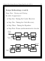
Five Day Schedule
• DAY 1 (3 lecture hours, 3 lab hours)
– A (Naive) Digital Radio
– (De)Modulation
– Automatic Gain Control
• DAY 2 (3 lecture hours, 3 lab hours)
– An Idealized RF System Simulation
– Carrier Recovery
• DAY 3 (3 lecture hours, 3 lab hours)
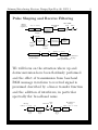
– Pulse Shaping and Receive Filtering
– Baud Timing for Clock Recovery
• DAY 4 (3 lecture hours, 3 lab hours)
– Linear Equalization
– Putting It All Together
• DAY 5 (6 lab hours)
– Design Project and Report Preparation
– Design Testing and Report Presentation
2
Johnson/Introducing Receiver Design/Apr-May 06: FOREWORD
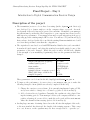
1
This compacted 5-day introduction to digital communication recevier design was originally extracted from C. R. Johnson, Jr. and W. A. Sethares, Telecommunication Breakdown: Concepts of Communication Transmitted via Software-Defined Radio (Prentice Hall,
2004) under the support of Prof. Rick Johnson by a Fulbright Scholarship to France in the
latter half of 2005. The accompanying labs were developed in collaboration with Dr. A.
G. Klein (currently a post-doctoral researcher in the Laboratoire de Signaux et Systemes,
Supélec, Gif sur Yvette, France). The first version of this compacted course was offered in
the ATHENS Programme at École Nationale Supérieure des Télécommunications (Paris,
France) in November 2005. The current version was prepared for presentation in April and
May 2006 at University College Dublin (Ireland) and Technische Universiteit Delft (the
Netherlands). This spring 2006 teaching activity is supported in part by a Stephen H.
Weiss Preisdential Fellowship from Cornell University.
In keeping with the philosophy of Telecommunication Breakdown, this compacted version is built around a Matlab-based software radio (developed by Dr. Andy Klein) that
implements the major digital signal processing operations of a common radio receiver:
demodulation, carrier recovery, matched receive filtering, baud-timing, equalization, and
decoding. This radio can compensate for the transmission impairments of carrier phase jitter, channel noise, time-varying channel intersymbol interference, and baud-timing offset.
Relying on a background in signals and systems comparable to that of J. H. McClellan, R.
W. Schafer, and M. A. Yoder, Signal Processing First (Pearson Prentice Hall, 2003), DAY
1 lectures present a basic pulse-amplitude-modulated (PAM) radio system and discuss how
such impairments, if uncompensated, can deteriorate communication system performance.
A basic adaptive algorithm creation strategy is described (in particular for automatic gain
control) to track the compensator parameter needed to counteract an encountered impairment, the specifics of which are initially unknown to the user and expected to be timevarying. DAY 2 lectures feature simulated system performance degradation due to various
impairments, and the successful automatic gain control compensation of flat fading. The
adaptive (stochastic gradient descent based) strategy is applied on DAY 2 to carrier phase
tracking by the receiver mixer (resulting in the popular phase-locked and Costas loop algorithms), on DAY 3 to baud timing for clock recovery (based on downsampled signal power
optimization), and on DAY 4 to equalization of frequency-selective channel impairments
(via both trained and blind schemes). DAY 5 consists of a final project assignment that
puts it all together.
The first 4 days are designed for 3 hours of lecture followed by 3 hours of supervised lab
instruction. There are no lectures on the 5th day, just a lab session, by the end of which
the modified radio developed individually by each student will be tested in comparison to
the base radio developed by Dr. Klein.
This course packet provides the overheads used in the lectures of days 1-4, the associated
lab assignments for days 1-4, the description of the final project, and a user’s manual for Dr.
Klein’s software radio. An accompanying CD includes the pertinent Matlab files (designed
for compatibility with version 6) for demonstrations cited in lecture, Dr. Klein’s software
radio, the labs, and final project. The CD also includes a pdf version of the printed course
packet. As a bonus, a movie is also included of a working receiver built (in the late 1980s) by
Applied Signal Technology for 16-QAM (where carrier phase offset results in rotation of the
recovered 4 by 4 constellation and carrier frequency offset results in recovered constellation
Johnson/Introducing Receiver Design/Apr-May 06: FOREWORD
2
rotation). A document, which is drawn from the CD accompanying Telecommunication
Breakdown and also includes a Matlab simulated radio, on the extension of the PAM radio
of Telecommunication Breakdown – and this compacted course – to the more pragmatic
QAM radio is also included on the CD for this compacted course, along with all of the
Matlab-based software for its simulation.
Johnson/Introducing Receiver Design/ Apr-May 06: DAY 1
DAY 1
• A (Naive) Digital Radio
• (De)Modulation
• Automatic Gain Control
1
Johnson/Introducing Receiver Design/ Apr-May 06: DAY 1
A (NAIVE) DIGITAL RADIO
? An Illustrative Digital Communication
System
? Transmitter and Transmitted Pulse Sequence
? Received Signal and Receiver
? Synchronization Issues
? Spectrum Sharing
? RF Communication System
? Practical Obstacles
? Analog/Digital Signal Processing Split
2
Johnson/Introducing Receiver Design/ Apr-May 06: DAY 1
An Illustrative Digital Communication
System
• Objective: Send text converted to a stream of
bits from place 1 to place 2 through the
analog medium in between.
• Coding: Use standard ASCII code to convert
text to bits (using 8 bits per character)
• Transmitter: Use sequence of scaled
rectangular pulses to convey bits singly, e.g.,
1 → +1 and 0 → −1 or in clusters, e.g.,
10 → +1, 01 → −1, 00 → +3, and 11 → −3.
We choose pairs, so groups of 8 bits become
clumps of 4 symbols.
• Receiver: Sample received pulse and convert
symbols to bits, e.g.,
1, 3, −1, 1, −3 → 1000011011, and then back
to text.
3
Johnson/Introducing Receiver Design/ Apr-May 06: DAY 1
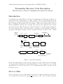
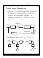
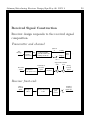
Transmitter and Transmitted Pulse
Sequence
• An idealized baseband transmitter
Symbols
s[k]
Text
Scaling
factor
Coder
Initiation
trigger
T-wide
analog
pulse
shape p(t)
generator
Baseband
signal y(t)
1
t 1 kT
and transmitted (baseband) signal
y(t)
3
1
t
21
23
t1T
Time, t
t 1 2T
t 1 3T
t 1 4T
• The transmitted signal consists of a sequence
of pulses, one corresponding to each symbol.
• Each pulse has the same rectangular shape
though offset in time and scaled in magnitude.
4
Johnson/Introducing Receiver Design/ Apr-May 06: DAY 1
5
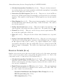
Received Signal and Receiver
• In the ideal case, the received signal is the
same as the transmitted signal though
attenuated in magnitude and delayed in time.
r(t)
3g
g
t1d
2g
t1d1T
Time, t
t 1 d 1 2T t 1 d 1 3T
23g
t 1 d 1 4T
• An idealized baseband receiver
Received
signal
Quantizer
h 1 kT
Sampler
Reconstructed
symbols
Decoder
Reconstructed
text
Johnson/Introducing Receiver Design/ Apr-May 06: DAY 1
Synchronization Issues
• Baud (symbol) timing
η selection for fixed T
top-dead-center
η = τ + δ + T /2
Peaked (rather than rectangular) pulse
shapes will reduce the spectral footprint of
the sequence of pulses, but increase the
sensitivity to top-dead-center baud-timing.
• Frame start determination
◦ grouping symbols to decoder
◦ example: −1, −1, 1, −3, −1; first 4 symbols
decode to “X” and last four decode to “a”
◦ special marker sequence inserted in source
sequence at start of a frame with
subsequent frame starts determined by
knowledge of the the period of their
recurrence.
6
Johnson/Introducing Receiver Design/ Apr-May 06: DAY 1
Spectrum Sharing
• Several user pairs should be able to
communicate through same medium
simultaneously in same geographical region.
• Interference avoidance achieved by
disallowing use of same frequencies by
different users in same geographical area.
• Bandwidth occupied by pulse shape/sequence
is inversely related to rectangle width.
• More frequent symbol transmission achieved
by narrower pulses increases exclusionary
baseband spectrum requirement.
• If all frequencies in bandlimited baseband
spectrum can be translated by same amount,
several users could be multiplexed to different
center frequencies without overlap.
7
Johnson/Introducing Receiver Design/ Apr-May 06: DAY 1
8
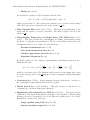
Radio Frequency (RF) Communication
System
• RF transmitter
Text
Symbols
Coder
Pulse
shape
filter
Baseband
signal
Frequency
translator
Passband
signal
• RF receiver
Received
signal
Frequency
translator
Baseband
signal
Sampler
Quantizer
Decoder
Reconstructed
text
Johnson/Introducing Receiver Design/ Apr-May 06: DAY 1
9
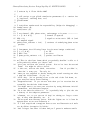
Practical Obstacles
• precise frequency translation required in
receiver
• precise timing required in receiver
• multi-user interference occurs in received
signal, e.g. since each user is not strictly
bandlimited in frequency
• noise contamination of transmitted signal:
in-band, out-of-band, narrowband, or
broadband
• channel distortion: fading or multipath,
possibly time-varying
Interference
from other sources
Transmitted
signal
Gain
with
delay
Received
signal
1
1
Self-interference
Multipath
Johnson/Introducing Receiver Design/ Apr-May 06: DAY 1
10
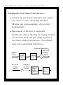
Analog/Digital Signal Processing Split
• Due to cost and flexibility benefits, modern
radio design is pushing the sampler (and
subsequent digital signal processing) closer to
the received signal, i.e. the output of the low
noise amplifier driven by the antenna signal.
Received
signal
Analog
signal
processing
h 1 kT
Digital
signal
processing
• Sample period ≤ symbol period.
Recovered
source
Johnson/Introducing Receiver Design/ Apr-May 06: DAY 1
An ASP/DSP Division of Labor
ASP:
• frequency translation to intermediate
frequency
• out-of-band signal attenuation
• automatic gain control
DSP:
• downconversion to baseband (via mixer)
• carrier tracking (via mixer phase setting)
• symbol timing (via interpolation)
• channel compensation (via linear filtering)
• symbol decision (via quantization)
• frame synchronization (via marker
correlation)
• decode symbols to message text (via table)
11
Johnson/Introducing Receiver Design/ Apr-May 06: DAY 1
(DE)MODULATION
? Up-Conversion via Mixing
? Downconversion via Mixing
? Message Recovery via Filtering
? Synchronized Demodulation of Amplitude
Modulation with Suppressed Carrier
? Unsynchronized Demodulation
? Sub-Nyquist Sampling of RF
? Interpolation
12
Johnson/Introducing Receiver Design/ Apr-May 06: DAY 1
Up-Conversion via Mixing
• For upconversion mixer multiplies input
waveform with a sinusoid
– s(t) = w(t)cos(2πfo t)
– w(t): message waveform
– s(t): transmitted waveform (mixer output)
• We want to compute the Fourier transform of
the transmitted waveform s(t) using:
◦ Exponential definition of a cosine
1 jx
cos(x) = (e + e−jx )
2
◦ Fourier transform definition
Z ∞
w(t)e−j2πf t dt = F {w(t)}
W (f ) =
−∞
13
Johnson/Introducing Receiver Design/ Apr-May 06: DAY 1
14
Up-Conversion via Mixing (cont’d)
• So:
S(f ) = F {s(t)} = F {w(t) cos(2πf0 t)}
1 j2πf t
−j2πf0 t
0
+e
= F w(t) 2 e
=
1 j2πf t
−j2πf t
−j2πf0 t
0
+e
w(t) 2 e
e
dt
−∞
R∞
1
2
=
R∞
−j2π(f −f0 )t
−j2π(f +f0 )t
w(t) e
+e
R
1 ∞
= 2 −∞ w(t) e−j2π(f −f0 )t dt
R
1 ∞
+ 2 −∞ w(t) e−j2π(f +f0 )t dt
−∞
= 21 W (f − f0 ) + 21 W (f + f0 )
uW(f)u
1
f†
2f †
f
(a)
uS(f)u
0.5
2f0 2 f † 2f0
f0
(b)
f0 1 f †
dt
Johnson/Introducing Receiver Design/ Apr-May 06: DAY 1
Downconversion via Mixing
• Assume transmitted signal arrives unimpaired
• For downconversion use mixer with frequency
and phase matching transmitter’s
d(t) = s(t) cos(2πf0 t) = w(t) cos2 (2πf0 t)
1
2
+ 12 cos(2x)
1 1
d(t) = w(t) 2 + 2 cos(4πf0 t)
= 12 w(t) + 21 w(t) cos(2π(2f0 )t)
cos2 (x) =
• Using linearity of Fourier transform and
previously extracted result on Fourier
transform of mixer output
D(f ) = F {d(t)}
= F { 21 w(t) + 21 w(t) cos(2π(2f0 )t)}
= 21 F {w(t)} + 21 F {w(t) cos(2π(2f0 )t)}
= 21 W (f ) + 41 W (f − 2f0 ) + 41 W (f + 2f0 )
15
Johnson/Introducing Receiver Design/ Apr-May 06: DAY 1
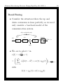
Message Recovery via Filtering
• Passing a signal s(t) through a linear system
with transfer function h(t) results in an
output that is the convolution of s(t) and
h(t).
• The Fourier transform of a convolution is the
product of the Fourier transforms.
• We often distinguish among linear systems
based on the range of frequencies they pass or
reject, e.g. lowpass, highpass, bandpass,
notch.
• The 12 W (f ) portion of D(f ) about zero
frequency can be extracted by filtering d(t)
through an ideal filter that has a flat
magnitude (and a linear phase) for low
frequencies and (near) zero magnitude for
high frequencies, i.e. an ideal lowpass filter.
16
Johnson/Introducing Receiver Design/ Apr-May 06: DAY 1
17
Message Recovery via Filtering (cont’d)
uW(f)u
2f
0
f
(a)
uS(f)u
2f0
f0
(b)
{S(t) . cos(2pfot)}
22f0
Lowpass filter
0
(c)
(a) original spectrum of the message
(b) message modulated by the carrier
(c) demodulated signal has original spectrum
after ideal lowpass filtering
2f0
Johnson/Introducing Receiver Design/ Apr-May 06: DAY 1
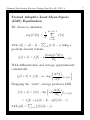
Synchronized Demodulation of Amplitude
Modulation with Suppressed Carrier
• analog message signal: w(t)
• transmitted/modulated signal:
v(t) = Ac w(t)cos(2πfc t)
• transmitted signal spectrum:
V (f ) =
1
1
Ac W (f + fc ) + Ac W (f − fc )
2
2
• ideal demodulation with synchronized mixing
and LPF:
1
m(t) = LPF{v(t)cos(2πfc t)} = Ac W (f )
2
• main disadvantage: carrier phase and
frequency synchronization needed at receiver
18
Johnson/Introducing Receiver Design/ Apr-May 06: DAY 1
19
Synchronized Demodulation of Amplitude
Modulation with Suppressed Carrier
(cont’d)
• Example: Perfect (delayed) recovery with
perfect synchronization using AM
Amplitude
3
2
1
0
21
Amplitude
(a) message signal
2
0
22
(b) message after modulation
Amplitude
3
2
1
0
21
(c) demodulated signal
Amplitude
3
2
1
0
21
0
0.01
0.02
0.03
0.04
0.05
0.06
0.07
(d) recovered message is a LPF applied to (c)
0.08
0.09
0.1
Johnson/Introducing Receiver Design/ Apr-May 06: DAY 1
Unsynchronized Demodulation
w(t)
v(t)
Ac cos(2pfct)
(a)
x(t)
v(t)
m(t)
LPF
cos(2p(fc + g)t + f)
(b)
(a) transmitter/modulator; (b) unsynchronized
receiver/demodulator
20
Johnson/Introducing Receiver Design/ Apr-May 06: DAY 1
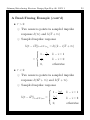
Unsynchronized Demodulation (cont’d)
• Using
F {g(t) cos(2παt + θ)}
1 jθ
−jθ
=
e G(f − α) + e G(f + α)
2
on
x(t) = v(t)cos(2π(fc + γ)t + φ)
and
1
1
V (f ) = Ac W (f + fc ) + Ac W (f − fc )
2
2
yields
Ac jφ
e {W (f + fc − (fc + γ))
X(f ) =
4
+W (f − fc − (fc + γ))}
+e−jφ {W (f + fc + (fc + γ))
+W (f − fc + (fc + γ))}]
Ac jφ
=
e W (f − γ) + ejφ W (f − 2fc − γ)
4
−jφ
−jφ
+e
W (f + 2fc + γ) + e
W (f + γ)
21
Johnson/Introducing Receiver Design/ Apr-May 06: DAY 1
22
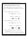
Unsynchronized Demodulation (cont’d)
• If no frequency offset (γ = 0), then with
exponential description of cosine
Ac jφ
(e + e−jφ )W (f )
X(f ) =
4
−jφ
jφ
+e W (f − 2fc ) + e
=
W (f + 2fc )
Ac
W (f )cos(φ)
2
Ac jφ
−jφ
+
e W (f − 2fc ) + e
W (f + 2fc )
4
Thus, with LPF cutoff between W (f )
bandwidth B and 2fc − B
Ac
m(t) = LPF{x(t)} =
w(t)cos(φ)
2
Recovered signal is attenuated relative to
perfectly synchronized demodulation.
As φ approaches π/2, recovered signal
vanishes.
Johnson/Introducing Receiver Design/ Apr-May 06: DAY 1
Unsynchronized Demodulation (cont’d)
• If no carrier offset (φ = 0),
X(f ) =
Ac
[W (f − γ) + W (f − 2fc − γ)
4
+W (f + 2fc + γ) + W (f + γ)]
Thus, with m(t) = LPF{x(t)}
Ac
[W (f − γ) + W (f + γ)]
M (f ) =
4
and using frequency shifting property of
multiplication by a cosine
Ac
m(t) =
w(t)cos(2πγt)
2
Recovered signal is low-frequency amplitude
modulated relative to perfectly synchronized
demodulation; periodically (every 1/γ sec) it
vanishes.
• Ergo: The need for carrier recovery
23
Johnson/Introducing Receiver Design/ Apr-May 06: DAY 1
Sub-Nyquist Sampling of RF Signal
• In a digital radio, the sampler can be after
analog demodulation to baseband or after
partial analog demodulation to an
intermediate frequency.
• With sampling after analog demodulation to
baseband, we can use the Nyquist sampling
theorem to select a sample rate that allows
perfect reconstruction of analog signal at any
point in time just from sampled values.
• If we sample before demodulation to
baseband, must we sample at (the much
higher) Nyquist rate for the RF signal to
achieve successful demodulation?
24
Johnson/Introducing Receiver Design/ Apr-May 06: DAY 1
Sub-Nyquist Sampling (cont’d)
With w(t) the input to an impulse sampler, the
output ws (t) is
ws (t) = w(t)
∞
X
k=−∞
δ(t − kTs )
Analog w(t) is multiplied point-by-point by a
pulse train
Signal w(t)
Pulse train
S d(t 2 kTs)
Impulse sampling
ws(t)
Point sampling
w[k] 5 w(kTs) 5 w(t)|t 5 kTs
25
Johnson/Introducing Receiver Design/ Apr-May 06: DAY 1
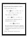
Sub-Nyquist Sampling (cont’d)
• With fs = 1/Ts
Ws (f ) = fs
∞
X
n=−∞
W (f − nfs )
Relative to W (f ), Ws (f ) has been scaled by
fs and contains replicas at every fs .
• Largest frequency in W (f ) less than fs /2 (top
plot) and slightly larger than f2 /2 (bottom)
26
Johnson/Introducing Receiver Design/ Apr-May 06: DAY 1
Sub-Nyquist Sampling (cont’d)
• Nyquist Sampling Theorem:
If the signal w(t) is bandlimited to B,
(W (f ) = 0 for all |f | > B) and if the
sampling rate is faster than fs = 2B, then
w(t) can be reconstructed exactly for all t
from its samples w(kTs ).
• Sub-Nyquist Sampling:
– What if the signal to be sampled is a
passband signal, but the signal to be
reconstructed is this passband signal
downconverted to a baseband signal with
a much lower maximum frequency?
– Can sub-Nyquist sampling of the passband
signal be employed without aliasing of the
baseband signal?
– The following examples provide a positive
answer.
27
Johnson/Introducing Receiver Design/ Apr-May 06: DAY 1
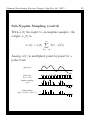
Sub-Nyquist Sampling (cont’d)
• Example:
– Consider fs = fc /2
uW(f)u
1
2B
B
f
(a)
uS(f)u
1/2
2fc2B
2fc
2fc1B
fc2B
fc
fc1B
f
(b)
uY(f)u
23fc/2
2fc
2fc/2
0
f
fc/2
(= fc2fs)
fc
3fc/2
(= fc1fs)
– Works for fs = fc /n
– What if fs not exactly fc /n?
28
Johnson/Introducing Receiver Design/ Apr-May 06: DAY 1
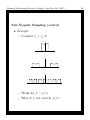
Sub-Nyquist Sampling (cont’d)
• Another Example: For a PAM system the
sampler, downconverter, and downsampler (to
symbol period T ) should produce an output
x8 with a spectrum matching that of a
sampled version (with sample period
matching symbol period) of the baseband
source x1 .
29
Johnson/Introducing Receiver Design/ Apr-May 06: DAY 1
Sub-Nyquist Sampling (cont’d)
Another Example (cont’d)
• For the following specifications in kHz
f1 = 50
f2 = 1690
f3 = 1920
f4 = 1460
f5 = 1620
f6 = 1760
f7 = 800
f8 = 90
f9 = 60
given |X1 (f )| as even-symmetric, triangular
shaped, and centered at zero frequency and
M = 2, we can draw |Xi (f )| for i = 1, 2, ..., 8
to show that |X8 (f )| matches (up to a scalar
gain factor) the magnitude spectrum of x1 (t)
sampled at the symbol rate.
30
Johnson/Introducing Receiver Design/ Apr-May 06: DAY 1
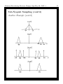
Sub-Nyquist Sampling (cont’d)
Another Example (cont’d)
31
Johnson/Introducing Receiver Design/ Apr-May 06: DAY 1
Sub-Nyquist Sampling (cont’d)
Another Example (cont’d)
32
Johnson/Introducing Receiver Design/ Apr-May 06: DAY 1
Interpolation
• Objective: Use signal samples from times kTs
to reconstruct the analog signal value at a
time instant not among the set of sample
times.
• Sinc interpolator:
w(t)|t=τ = w(τ ) =
Z
∞
ρ=−∞
ws (ρ)sinc(τ − ρ)dρ
Because ws (ρ) is nonzero only when ρ = kTs ,
w(τ ) =
∞
X
k=−∞
ws (kTs )sinc(τ − kTs )
• Prescription for perfection: As long as
fs > 2B (where B is the highest frequency
present in w(t)) this (doubly infinite) sinc
interpolator is exact.
• Filtering interpretation: Creation of w(τ ) can
be interpreted as a convolution of ws with a
sinc-shaped impulse response.
33
Johnson/Introducing Receiver Design/ Apr-May 06: DAY 1
Interpolation (cont’d)
• Ideal LPF Interpolator: Convolution in time
domain is multiplication in frequency domain.
Spectrum of sinc is a rectangle, i.e. an ideal
LPF. Thus, an ideal lowpass filter with
appropriate cutoff frequency is a perfect
interpolator for a Nyquist-sampled signal.
• Perfection inhibiting practicalities: In
practice, it is necessary to truncate the doubly
infinite convolutional sum. Furthermore, w(t)
can always be expected to have traces of
frequencies above B. Therefore, in practice,
we must settle for an approximation.
• Non-ideal LPF interpolator: Fortunately, any
suitable LPF (with nonzero, flat magnitude
and linear phase up to frequency B and fully
rejecting before reaching next higher
frequency chunk in spectrum of ws ) will
provide accurate interpolation.
34
Johnson/Introducing Receiver Design/ Apr-May 06: DAY 1
35
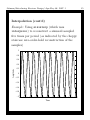
Interpolation (cont’d)
Example: Using sininterp (which uses
interpsinc) to reconstruct a sinusoid sampled
five times per period (as indicated by the choppy
staircase zero-order-hold reconstruction of the
samples)
1
0.8
0.6
Amplitude
0.4
0.2
0
20.2
20.4
20.6
20.8
21
10
10.05
10.1
10.15
10.2
10.25
Time
10.3
10.35
10.4
10.45
10.5
Johnson/Introducing Receiver Design/ Apr-May 06: DAY 1
AUTOMATIC GAIN CONTROL
? Automatic Gain Control Algorithm
Construction
? Tracking Example: Time-Varying Fade
36
Johnson/Introducing Receiver Design/ Apr-May 06: DAY 1
Sampling with AGC
We now focus on the sampler and its surrounding
automatic gain control (AGC) in a receiver front
end
Antenna
Sampler
BPF
Analog
received
signal
Analog
r(t)
conversion
to IF
a
AGC
s(kTs) 5 s[k]
Quality
Assessment
Our purpose here is more to introduce a strategy
for parameter adaptation that will be repeated for
carrier and clock recovery and equalization, rather
than to promote a particular AGC algorithm.
37
Johnson/Introducing Receiver Design/ Apr-May 06: DAY 1
Automatic Gain Control (AGC)
• An AGC maintains the dynamic range of a
(zero-average) signal by attenuating when it
is too large (as in (a)) and by amplifying
when too small (as in (b)).
(a)
(b)
• AGC adjusts gain parameter a so average
energy at output remains (roughly) fixed,
despite fluctuations in average received
energy.
Sampler
r(t)
a
s(kT) 5 s[k]
Quality
Assessment
38
Johnson/Introducing Receiver Design/ Apr-May 06: DAY 1
AGC (cont’d)
Gain Tuning:
• We are to choose a for a received waveform
r(t) segment that produces sampler outputs
s[k] with the intent of having the average s2
value over that dataset match a preselected
constant d2 .
• Because s[k] = ar(kTs ), we can choose
a = d2
=
PN 2
avg{r 2 [k]}
r
[k
+
i]
i=1
d2
2
1
N
(preferring a > 0) to make (as desired)
N
1 X 2
{
s [k + i]} = d2
N i=1
• Unfortunately, we need the samples of r,
which are not available on the DSP side of
the receiver, to solve this formula for a.
• Our search for a gain tuner continues.
39
Johnson/Introducing Receiver Design/ Apr-May 06: DAY 1
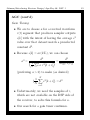
AGC (cont’d)
Heuristic Algorithm Development:
As an alternative, consider the following strategy:
• select an initial positive a.
• As a sample s arrives, compare its square to
d2 .
• If s2 at that particular sample instant is
greater than d2 , we will reduce a positive a to
a smaller positive value. If a is negative, we
would decrease its magnitude, i.e. increase it
toward zero.
• Plus, the correction term should be larger the
further d2 is from s2 .
• Similarly, if s2 < d2 , we will increase a
positive a by an amount proportional to
d2 − s2 . If a is negative, a should be
decreased (i.e. made more negative), so its
magnitude increases.
40
Johnson/Introducing Receiver Design/ Apr-May 06: DAY 1
AGC (cont’d)
An algorithm that performs this strategy is
a[i + 1] = a[i] + µ{sign(a[i])}(d2 − s2 [i])
where µ is a suitably small positive stepsize. (The
sign(a[i]) term can be removed if a[i] starts and
stays positive.)
• Can this algorithm be implemented from data
available on the DSP side of the sampler?
Ans: Yes, s (and not r) is needed
• Will this
converge to the desired a
q algorithm
PN 2
1
of ±d/ N i=1 r [i]?
Ans: It depends what you mean by
“converge”.
41
Johnson/Introducing Receiver Design/ Apr-May 06: DAY 1
AGC (cont’d)
• The candidate algorithm
a[i + 1] = a[i] + µ{sign(a[i])}(d2 − s2 [i])
cannot be expected to converge to a fixed
value.
• Because r ranges widely, only on average does
a2 r 2 (or s2 ) actually equal d2 .
• The resulting (typically) nonzero
instantaneous error in d2 − s2 and a
nonvanishing stepsize µ will result in a change
in a even if it is already at the right value for
the average behavior of s2 .
• A sufficiently small µ should keep this
asymptotic rattling within a tolerable level.
42
Johnson/Introducing Receiver Design/ Apr-May 06: DAY 1
AGC (cont’d)
Testing:
• Using agcgrad with avg{r 2 } ≈ 1 and
√
2
d = 0.15, the desired a ≈ 0.15 ≈ 0.38.
• Start at x = 2 with µ = 0.001
Adaptive gain parameter
2
1.5
1
0.5
0
0
1000
2000
3000
4000 5000 6000
Input r(k)
7000
8000
9000 10000
0
1000
2000
3000
4000 5000 6000
Output s(k)
7000
8000
9000 10000
0
1000
2000
3000
4000 5000 6000
Iterations
7000
8000
9000 10000
5
0
25
5
0
25
• Start of x = −2 with µ = 0.001
Adaptive gain parameter
0
−0.5
−1
−1.5
−2
0
1000
2000
3000
4000
0
1000
2000
3000
4000
0
1000
2000
3000
4000
5000
Input r(k)
6000
7000
8000
9000
10000
5000
6000
Output s(k)
7000
8000
9000
10000
7000
8000
9000
10000
5
0
−5
5
0
−5
5000
iterations
6000
43
Johnson/Introducing Receiver Design/ Apr-May 06: DAY 1
AGC (cont’d)
• Start at x = 0.05 with µ = 0.001
Adaptive gain parameter
2
1.5
1
0.5
0
0
1000
2000
3000
4000
0
1000
2000
3000
4000
0
1000
2000
3000
4000
5000
Input r(k)
6000
7000
8000
9000
10000
5000
6000
Output s(k)
7000
8000
9000
10000
7000
8000
9000
10000
5
0
−5
5
0
−5
5000
iterations
6000
• Start at x = 2 with µ = 0.02
Adaptive gain parameter
2
1.5
1
0.5
0
0
1000
2000
3000
4000
0
1000
2000
3000
4000
0
1000
2000
3000
4000
5000
Input r(k)
6000
7000
8000
9000
10000
5000
6000
Output s(k)
7000
8000
9000
10000
7000
8000
9000
10000
5
0
−5
5
0
−5
5000
iterations
6000
44
Johnson/Introducing Receiver Design/ Apr-May 06: DAY 1
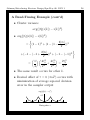
AGC (cont’d)
Observations:
• Asymptotically, this algorithm hovers in a
small region about the desired answer.
• The asymptotic hovering region’s size can be
decreased by reducing the stepsize µ, which
also reduces the algorithm convergence rate.
• When the average value of the hovering
parameter has effectively reached a fixed
value, the average of a[i + 1] will equal the
average of a[i] such that from our algorithm
a[i + 1] = a[i] + µsign(a[i])(d2 − s2 [i])
the average of the correction term
µsign(a[i])(d2 − s2 [i]) must be zero.
• With µ > 0 and the asymptotic hovering a[i]
not changing sign, zeroing the average
correction term zeros the average of d2 − s2 .
But, indeed that is what we seek.
45
Johnson/Introducing Receiver Design/ Apr-May 06: DAY 1
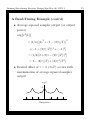
AGC (cont’d)
Gradient Descent Algorithm Development:
• As a more generalizable approach to adaptor
algorithm development consider specifying a
cost function and using an iterative optimizer
based on gradient descent
∂JN (a)
|a=a[i]
a[i + 1] = a[i] − µ
∂a
• Try JN (a) = avg{|a|((s2 [k]/3) − d2 )} with the
definition of “avg” as
avg{x[k]} = (1/N )
k−N
X+1
x[i]
i=k
• For small stepsize µ, differentiation and
averaging are approximately interchangeable
2 2
∂JN (a)
∂
a r (kT )
=
[avg{|a|
− d2 }]
∂a
∂a
3
2 2
a r (kT )
∂
− d2 ]}
≈ avg{ [|a|
∂a
3
46
Johnson/Introducing Receiver Design/ Apr-May 06: DAY 1
AGC (cont’d)
• With
∂|a|
∂a
= sign(a) and
dw
dx
=
dw
dy
·
dy
dx
∂JN (a)
≈ avg{|a|(1/3)2ar 2 (kT )
∂a
+sign(a)(1/3)a2 r 2 (kT )} − sign(a)d2
• With sign(a)|a| = a
∂JN (a)
2 2
2
≈ avg{sign(a) a r (kT ) − d }
∂a
• With a2 r 2 = s2
∂JN (a)
2
2
≈ avg{sign(a) s [k] − d }
∂a
So, the stationary points of zero gradient are
in the right places with avg{s2 } = d2 .
• With ∂(sign(a))/∂a = 0 everywhere but
a = 0, the second derivative is approximately
∂ 2 2
2
sign(a) a r (kT ) − d }
avg{
∂a
= avg{2a sign(a)r 2 (kT )} = avg{2|a|r 2 (kT )} > 0
So, stationary points at a 6= 0 are minima.
47
Johnson/Introducing Receiver Design/ Apr-May 06: DAY 1
48
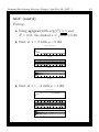
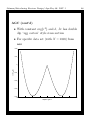
AGC (cont’d)
• With constant avg{r 2 } and d, JN has double
dip “egg carton” style cross section
• For specific data set (with N = 1000) from
aes
0.02
0.01
N
cost J (a)
0
−0.01
−0.02
−0.03
−0.04
−0.8
−0.6
−0.4
−0.2
0
adaptive gain a
0.2
0.4
0.6
0.8
Johnson/Introducing Receiver Design/ Apr-May 06: DAY 1
AGC (cont’d)
• Computation of the gradient requires that a
remain constant over the N samples over
which avg{s2 } is composed.
• Consider squeezing the averaging window to a
single sample so N = 1 and
2
2
a[i + 1] = a[i] − µsign(a[i]) s[i] − d
• This is the algorithm developed heuristically
and tested previously.
• This algorithm also emerges from first
reducing the averaging window to N = 1 in
the cost function and then taking the gradient
and forming a gradient descent iteration.
• This technique of shrinking the averaging
window so averaging is explicitly removed
works because LPF action of adaptation acts
similarly to averaging before updating.
49
Johnson/Introducing Receiver Design/ Apr-May 06: DAY 1
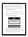
Tracking Example: Time-Varying Fade
• To demonstrate desired tracking capability,
use agcvsfading to test
2
2
a[i + 1] = a[i] − µsign(a[i]) s[i] − d
with µ = 0.01, d2 = 0.5, a[1] = 1, and a large,
slow, oscillating channel gain
Input r(k)
5
0
25
0
0.5
1
1.5
2
2.5
3
3.5
4
4.5
5
3 104
Adaptive gain parameter
1.5
1
0.5
0
0
0.5
1
1.5
2
2.5
Output s(k)
3
3.5
4
4.5
5
3 104
0
0.5
1
1.5
2
2.5
Iterations
3
3.5
4
4.5
5
3 104
5
0
25
• Fade must be changing sufficiently slowly and
the input must never die for the AGC with
small stepsize to track adequately.
50
Johnson/Introducing Receiver Design/Apr-May 06: DAY 1 LAB
1
Laboratory Exercises – Day 1
Introduction to Digital Communication Receiver Design
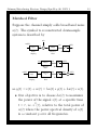
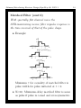
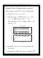
Task 1: Filter Design With remez
The Matlab command remez is useful for generating so-called “equiripple FIR filters”. We
will rely on it frequently for designing lowpass and bandpass filters. The remez command
takes three parameters. Type help remez to familiarize yourself with the parameters –
you only need to pay attention to the first paragraph in the help, called with 3 parameters
N,F, and A.
The following code generates 3 seconds worth of a random (white) signal sampled at 10
kHz, and plots the magnitude spectrum:
time=3;
Ts=1/10000;
x=randn(time/Ts,1);
plotspec(x,Ts);
The following lines design a 100-th order low-pass filter with a cutoff at 1 kHz, and plots
the filtered signal:
h=remez(100,[0 0.2 0.21 1],[1 1 0 0])’;
y=filter(h,1,x);
plotspec(y,Ts);
Your task: Provide the corresponding lines of code to design a bandpass filter (BPF)
which passes frequencies between 1.5 kHz and 2.5 kHz. Plot the result of filtering x with
the BPF. Plot the result of filtering y with the BPF.
Task 2: Filtering with Tapped Delay Lines
The filter and conv commands are quite useful for filtering signals, but they assume you
have all of the data available. In a real-time communication system, we may want to put
each sample into a filter as we receive it. In this case, the filter and conv commands are
not so useful. For a signal x[n] passing through a filter h[n] of length N, the output at
time n is given by the convolution sum:
y[n] =
N
−1
X
h[k]x[n − k]
k=0
We can implement the convolution sum very efficiently in Matlab using vector inner
products. For example, the filter output at time n is given by
y(n)=h’*x(n:-1:n-N);
Johnson/Introducing Receiver Design/Apr-May 06: DAY 1 LAB
2
Your task: Using for loops and vector inner products, write a few lines of code that
are equivalent to the command y=filter(b,1,x). Compare your result with the the
previous problem where you used the filter command, and calculate the mean squared
error between the two (Note: you may ignore the first N samples in the error calculation,
where N is the number of taps in the filter).
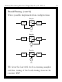
Task 3: Detection via Correlation
In packet-based wireless communication systems, the beginning of the transmission usually
contains a marker sequence. The receiver is constantly looking for such a marker sequence;
when it detects that a marker sequence has been sent, it knows that data is about to be
transmitted, and it knows the location of the “start” of the packet.
The standard technique for identifying a marker sequence is called correlation. Correlation is much like convolution, but with a sign change in the indexing. If y[n] is the received
signal, marker[n] is the (known) marker sequence of length N, the correlator output z at
time n is given by
z[n] =
N
−1
X
marker[k]y[n + k].
k=0
When the correlator output z[n] exceeds some pre-determined threshold, the receiver decides that the marker was identified at that value of n.
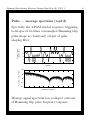
Your task: Load the file /day1/correl ex.mat by typing load correl ex. This
file contains two variables: a length 100 marker sequence called marker, and a length
2000 received sequence called y. Write a few lines of code to perform the correlation and
determine the starting location of the marker sequence. Also, show a plot of z[n].
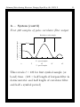
Task 4: Amplitude Modulation
Consult the file /day1/AM.m. This code generates a message w(t) and modulates it with a
carrier at frequency fc . The demodulation is done with a cosine of frequency fc + γ and
a phase offset of φ. When γ = 0 and φ = 0 (i.e. in the ideal conditions), the output is
identical to the original message, except for the inevitable delay caused by the linear filter.
Your tasks:
1. Plot the signals w(t), v(t), x(t), and m(t), and describe what you see.
2. Using the plotspec command, plot the spectra of these same signals. Describe what
you see.
3. Change the phase offset, φ. Describe the effect for different values.
4. Change the frequency offset, γ. Describe the effect for different values.
Johnson/Introducing Receiver Design/Apr-May 06: DAY 1 LAB
3
Task 5: Sinc Interpolation
As you should be aware, sampling a signal faster than the Nyquist rate allows for perfect
reconstruction since no information is lost. However, once we have a sampled digital signal,
how do we reconstruct the data between samples? The answer is sinc interpolation.
We will use sinc interpolation quite often in our digital receiver, particular during baudtiming. The function /day1/interpsinc.m performs sinc interpolation, and we will use
this frequently. Open this file, and familiarize yourself with its operation.
To see an example of using sinc interpolation, consider interpolating the points of a sampled sinusoid. The file /day1/interp example.m generates a sine wave w(t) of frequency
20 Hz with a sampling rate of 100 Hz. The code then shows how to use interpsinc.m to
interpolate between the samples.
Your task: Generate a new wave w(t) which is the sum of 2 sinusoids – one with
frequency 17 Hz, and one with frequency 20 Hz. Consider t between -10 and 10. Let w(kTs )
represent samples of w(t) with Ts = 0.01. Use interpsinc.m to interpolate the values
w(0.011), w(0.013), and w(0.015), using 10× oversampling. Compare the interpolated
values to the actual values.
Task 6: Automatic Gain Control via Gradient Descent
The function /day1/agcgrad.m implements the AGC gradient descent algorithm which
minimizes the cost
(
a2 r 2
JN (a) = avg |a|
− ds
3
!)
by choice of a. The gain parameter a adjusts automatically to make the overall power of
the output s roughly equal to the specified parameter ds. Run agcgrad.m and you will see
that a converges to about 0.38 since 0.382 ≈ 0.15 = ds2 .
Your task: Using agcgrad.m, answer the following questions
1. What range of stepsize mu works? What happens if it is too small? too large?
2. How does choice of mu effect convergence rate?
3. How does the variance of the input effect the convergent value of a?
4. Try initializing the estimate a(1)=-2. Which minimum does the algorithm find?
What happens to the data record?
Johnson/Introducing Receiver Design/Apr-May 06: DAY 2
DAY 2
• RF System Simulation with
Impairments
• Carrier Recovery
1
Johnson/Introducing Receiver Design/Apr-May 06: DAY 2
AN IDEALIZED RF SYSTEM
SIMULATION
? A Naive/Ideal Communication System
? Flat Fading
? What if ...
2
Johnson/Introducing Receiver Design/Apr-May 06: DAY 2
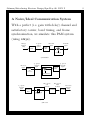
3
A Naive/Ideal Communication System
With a perfect (i.e. gain with delay) channel and
satisfactory carrier, baud timing, and frame
synchronization, we simulate this PAM system
(using idsys).
T - spaced
symbol
sequence
Message
character
string
Baseband
signal
Passband
signal
Pulse
filter
Coder
cos(2pfc t)
Mixer
(a) Transmitter
Ts - spaced
passband
signal
Received
signal
Lowpass
filter
Ts - spaced
baseband
signal
kTs
k 5 0, 1, 2, ...
cos(2pfc kTs)
Mixer
Sampler
Demodulator
Ts - spaced
baseband
signal
MTs - spaced
soft
decisions
Pulse
correlator
filter
MTs - spaced
hard
decisions
Quantizer
n(MTs) 1 lTs
n 5 0, 1, 2, ...
Downsampler
(b) Receiver
Decoder
Recovered
character
string
Johnson/Introducing Receiver Design/Apr-May 06: DAY 2
A ... System (cont’d)
TRANSMITTER
• text message: 01234 I wish I were an Oscar
Meyer wiener 56789
• coding: text characters via 8-bit ASCII to
4-PAM m[i]
• baud interval: T = 1 time unit
• pulse shape: T -wide Hamming blip p(·)
• carrier frequency: fc = 20
• carrier phase: 0
RECEIVER
• sampler period: Ts (= T /M )
• oversample rate: M = 100
4
Johnson/Introducing Receiver Design/Apr-May 06: DAY 2
A ... System (cont’d)
• free running sampler output:
r(t)|t=kTs =
N
−1
X
m[i]p(kTs − iT )cos(2πfc kTs )
i=0
• mixer frequency: fc = 20
• mixer phase: 0
• demodulator LPF: remez(fl,fbe,damps)
with fl = 50, fbe = [ 0 0.5 0.6 1 ], and damps
=[1100]
• pulse correlator filter: T -wide Hamming blip
• downsampler baud timing: ` = 125
(determined experimentally)
• quantizer: to nearest element in {±1, ±3}
• decoder: 4-PAM to 8 bits via reverse ASCII
to text (with frame synchronization assured
by indexing from first symbol set by baud
timing)
5
Johnson/Introducing Receiver Design/Apr-May 06: DAY 2
6
A ... System (cont’d)
Transmitter baseband signal and magnitude
spectrum
3
Amplitude
2
1
0
21
22
23
0
20
40
60
80
100
Seconds
120
140
160
180
200
0
250
240
230
220
210
0
Frequency
10
20
30
40
50
10000
Magnitude
8000
6000
4000
2000
Note that spectrum is limited to minus to plus
Nyquist frequency, i.e. half of oversample
frequency.
Johnson/Introducing Receiver Design/Apr-May 06: DAY 2
7
A ... System (cont’d)
Transmitter passband signal and magnitude
spectrum
3
Amplitude
2
1
0
21
22
23
0
20
40
60
80
100
Seconds
120
140
160
180
200
0
250
240
230
220
210
0
Frequency
10
20
30
40
50
5000
Magnitude
4000
3000
2000
1000
Johnson/Introducing Receiver Design/Apr-May 06: DAY 2
8
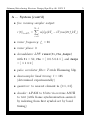
A ... System (cont’d)
Receiver mixer output and magnitude spectrum
3
Amplitude
2
1
0
21
22
23
0
20
40
60
80
100
Seconds
120
140
160
180
200
0
250
240
230
220
210
0
Frequency
10
20
30
40
50
5000
Magnitude
4000
3000
2000
1000
Johnson/Introducing Receiver Design/Apr-May 06: DAY 2
9
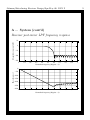
A ... System (cont’d)
Receiver post-mixer LPF frequency response
Magnitude response (dB)
50
0
250
2100
2150
0
0.1
0.2
0.3
0.4
0.5
0.6
0.7
Normalized frequency (Nyquist 5 1)
0.8
0.9
1
0
0.1
0.2
0.3
0.4
0.5
0.6
0.7
Normalized frequency (Nyquist 5 1)
0.8
0.9
1
0
Phase (degrees)
2500
21000
21500
22000
22500
23000
Johnson/Introducing Receiver Design/Apr-May 06: DAY 2
10
A ... System (cont’d)
Receiver downconverter-LPF output and
magnitude spectrum
3
Amplitude
2
1
0
21
22
23
0
20
40
60
80
100
Seconds
120
140
160
180
200
0
250
240
230
220
210
0
Frequency
10
20
30
40
50
10000
Magnitude
8000
6000
4000
2000
Johnson/Introducing Receiver Design/Apr-May 06: DAY 2
11
A ... System (cont’d)
First 400 samples of pulse correlator filter output
Amplitude of received signal
Best times to take samples
Delay
3
2
1
0
21
22
23
0
0
50
100
150
200
250
Ts - spaced samples
300
T
2T
T - spaced samples
3T
350
400
4T
This reveals ` = 125 for first symbol sample (or
baud) time. (125 = half length of lowpass filter in
downconverter and half length of correlator filter
and half a symbol period)
Johnson/Introducing Receiver Design/Apr-May 06: DAY 2
12
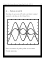
A ... System (cont’d)
Overlay of successive 4T -wide correlator output
segments starting on first baud time
4
3
2
1
0
21
22
23
24
0
50
100
150
200
250
300
350
Note recurrence of pulse peaks at successive
T -wide intervals.
400
Johnson/Introducing Receiver Design/Apr-May 06: DAY 2
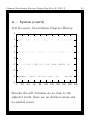
A ... System (cont’d)
Soft Decisions Constellation Diagram History
4
3
2
1
0
21
22
23
24
0
20
40
60
80
100 120 140 160 180 200
Because the soft decisions are so close to the
alphabet levels, there are no decision errors and
no symbol errors.
13
Johnson/Introducing Receiver Design/Apr-May 06: DAY 2
Flat Fading
Impairment: At time representing 20% of
duration of simulation window, the channel gain
changes abruptly from 1 to 0.5. (as in idsys+agc)
Effect: Soft decisions in “ideal” system receiver
3
2
1
0
21
22
23
24
0
20
40
60
80 100 120 140 160 180 200
The soft decisions have all moved inside 2 in
magnitude, meaning that decision device will
never produce ±3 ⇒ lots of errors.
14
Johnson/Introducing Receiver Design/Apr-May 06: DAY 2
Flat Fading (cont’d)
Fixed: Soft decisions with inclusion of AGC
4
3
2
1
0
21
22
23
24
0
20
40
60
80
100 120 140 160 180 200
Decisions correct once top and bottom stripes in
constellation diagram history have magnitude
> 2.
15
Johnson/Introducing Receiver Design/Apr-May 06: DAY 2
Flat Fading (cont’d)
Adapted gain time history: Starts at 1; ends near
2.
2.6
2.4
2.2
2
1.8
1.6
1.4
1.2
1
0.8
0
0.2 0.4 0.6 0.8
1
1.2 1.4 1.6 1.8 2
3104
16
Johnson/Introducing Receiver Design/Apr-May 06: DAY 2
17
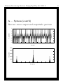
What if ...
Channel noise: Noisy received signal and
spectrum (from impsys)
Amplitude
5
0
25
0
20
40
60
80
100 120 140 160 180
Seconds
200
Magnitude
5000
4000
3000
2000
1000
0
10
250 240 230 220 210 0
Frequency
20
30
40
50
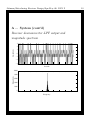
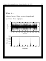
Johnson/Introducing Receiver Design/Apr-May 06: DAY 2
18
What if ... (cont’d)
Channel noise (cont’d): Received signal eye
diagram of 4 symbol wide overlays
5
4
3
2
1
0
21
22
23
24
25
0
50
100
150
200
250
300
350
400
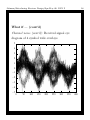
Johnson/Introducing Receiver Design/Apr-May 06: DAY 2
19
What if ... (cont’d)
Channel noise (cont’d): Pulse correlator filter
synchronized output signal
4
3
2
1
0
21
22
23
24
0
50
100
150
200
250
300
350
400
Johnson/Introducing Receiver Design/Apr-May 06: DAY 2
20
What if ... (cont’d)
Multipath: Mild multipath soft decisions
4
3
2
1
0
21
22
23
24
0
20
40
60
80
100
120
140
160
180
200
The appearance of 4 distinct stripes indicates no
decision errors.
Johnson/Introducing Receiver Design/Apr-May 06: DAY 2
21
What if ... (cont’d)
Multipath (cont’d): Harsh multipath soft decisions
4
3
2
1
0
21
22
23
24
0
20
40
60
80
100
120
140
160
180
200
The lack of emergence of 4 distinct stripes
indicates the (likely) presence of decision errors.
Johnson/Introducing Receiver Design/Apr-May 06: DAY 2
22
What if ... (cont’d)
Carrier phase offset: Severe offset
2
1.5
1
0.5
0
20.5
21
21.5
22
0
20
40
60
80
100
120
140
160
180
200
The attenuation due to carrier phase offset
reduces all soft decisions below magnitude 2
resulting in no ±3 as decision device outputs ⇒
plenty of errors.
If scaled back up so stripes of largest magnitude
values are above magnitude 2, the SNR will suffer
relative to case without carrier phase offset.
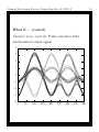
Johnson/Introducing Receiver Design/Apr-May 06: DAY 2
23
What if ... (cont’d)
Carrier frequency offset: Soft decisions for 0.01%
frequency offset
3
2
1
0
21
22
23
0
20
40
60
80
100
120
140
160
180
200
The carrier frequency offset appears as a low
frequency amplitude modulation of the desired
outputs.
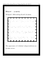
Johnson/Introducing Receiver Design/Apr-May 06: DAY 2
24
What if ... (cont’d)
Downsampler timing offset: Eye diagram with
debilitating offset
Assumed "best times" to take samples
3
2
1
0
21
22
23
0
50
100
150
200
250
300
350
400
With samples for symbol values taken every 100
samples after sample 125, numerous errors occur.
Johnson/Introducing Receiver Design/Apr-May 06: DAY 2
25
What if ... (cont’d)
Downsampler period offset: Eye diagram (top)
and soft decisions (bottom) with 1% downsampler
period offset
3
2
1
0
21
22
23
3
2
1
0
21
22
23
0
0
50
20
All is lost...
100
40
60
150
80
200
250
300
350
400
100 120 140 160 180 200
Johnson/Introducing Receiver Design/Apr-May 06: DAY 2
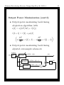
Well, then...
• Coding and matched receive filtering are
intended to counter effects of broadband
channel noise.
• Equalization compensates for multipath
interference, and can reject narrowband
interferers as well.
• Carrier recovery schemes (including phase
locked loops and Costas loops) adjust receiver
oscillator phase to counteract phase offset
(and mild frequency offset).
• Timing recovery (using interpolation) is
intended for reduction of downsampler timing
offset (and mild period offset).
26
Johnson/Introducing Receiver Design/Apr-May 06: DAY 2
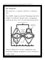
27
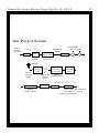
Our Project System
Binary
message
sequence b
we{23, 21, 1, 3}
Analog
upconversion
Carrier
specification
P(f)
Coding
Pulse
shaping
Transmitted
signal
Channel
Other FDM
Noise
users
1
1
Antenna
Analog
received
signal
Analog
conversion
to IF
Ts
Carrier
Input to the
synchronization
software
receiver
T
Downsampling
Timing
synchronization
Digital downconversion
to baseband
m
Equalizer
Pulse
matched
filter
Q(m)e{23, 21, 1, 3}
Decision
^
b
Decoding
Source and Reconstructed
error coding
message
frame synchronization
Johnson/Introducing Receiver Design/Apr-May 06: DAY 2
CARRIER RECOVERY
? Carrier Phase Tracking
? Adaptive Algorithm Development
? Carrier Extraction
? Phase-locked Loop
? Costas Loop
28
Johnson/Introducing Receiver Design/Apr-May 06: DAY 2
29
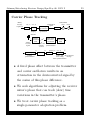
Carrier Phase Tracking
Binary
message
sequence b
we{23, 21, 1, 3}
Analog
upconversion
Carrier
specification
P(f)
Coding
Pulse
shaping
Transmitted
signal
Channel
Other FDM
Noise
users
1
1
Antenna
Analog
received
signal
Analog
conversion
to IF
Ts
Carrier
Input to the
synchronization
software
receiver
m
T
Downsampling
Timing
synchronization
Digital downconversion
to baseband
Equalizer
Pulse
matched
filter
Q(m)e{23, 21, 1, 3}
Decision
^
b
Decoding
Source and Reconstructed
error coding
message
frame synchronization
• A fixed phase offset between the transmitter
and carrier oscillators results in an
attenuation in the downconverted signal by
the cosine of this phase difference.
• We seek algorithms for adjusting the receiver
mixer’s phase that can track (slow) time
variations in the transmitter’s phase.
• We treat carrier phase tracking as a
single-parameter adaptation problem.
Johnson/Introducing Receiver Design/Apr-May 06: DAY 2
Adaptive Algorithm Development
Our (single-parameter) adaptive algorithm
development strategy:
• Propose a cost function assessing behavior
over measured data set.
• Check location of minima and maxima in
terms of adjusted parameter to see if in
desired location.
• Pursue (small stepsize) gradient descent
strategy (with its commutability of averaging
and differentiation). The correction term
must be calculable from available signals.
• Test performance.
30
Johnson/Introducing Receiver Design/Apr-May 06: DAY 2
Carrier Extraction
• For AM with suppressed carrier we will
process the received upconverted signal
r(kTs ) = s(kTs )cos(2πf0 kTs + φ)
which does not include an additive carrier, in
order to extract a signal related to the carrier.
• Consider squaring the received signal and
using cos2 (x) = (1/2)(1 + cos(2x)) to produce
r 2 (kTs ) =
(1/2)s2 (kTs )[1 + cos(4πf0 kTs + 2φ)]
31
Johnson/Introducing Receiver Design/Apr-May 06: DAY 2
Carrier extraction (cont’d)
• Rewrite s2 (t) as the sum of its (positive)
average value and the variation about this
average s2 (kTs ) = s2avg + v(kTs ), so
1 2
r (kTs ) = s (kTs )[1 + cos(4πf0 kTs + 2φ)]
2
2
= (1/2)[s2avg + v(kTs ) + s2avg cos(4πf0 kTs + 2φ)
+v(kTs )cos(4πf0 kTs + 2φ)]
• A narrow bandpass filter centered at 2f0 with
phase shift ρ at 2f0 extracts
x(kTs ) = (1/2)s2avg cos(4πf0 kTs + 2φ + ρ)
from r 2 while passing a bit of v about 2f0 .
• Digital BPF implementation presumes that
2f0 lies within the Nyquist frequency 1/(2Ts ).
32
Johnson/Introducing Receiver Design/Apr-May 06: DAY 2
33
Carrier Extraction (cont’d)
For 1 second of a 4-PAM signal with Hamming
blip symbol width T = 0.005, sample period (with
an oversample factor of 50) Ts = 0.0001, and a
carrier with frequency f0 = 1000 and phase
φ = −1, (from pllcrt) the received signal and its
spectrum are
3
amplitude
2
1
0
−1
−2
−3
0
0.1
0.2
0.3
0.4
0.5
seconds
0.6
0.7
0.8
0.9
1
0
−5000
−4000
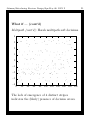
−3000
−2000
−1000
0
frequency
1000
2000
3000
4000
5000
1200
magnitude
1000
800
600
400
200
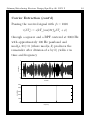
Johnson/Introducing Receiver Design/Apr-May 06: DAY 2
34
Carrier Extraction (cont’d)
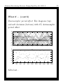
Passing the received signal with f0 = 1000
r(kTs ) = s(kTs )cos(2πf0 kTs + φ)
through a squarer and a BPF centered at 2000 Hz
with approximately 100 Hz passband and
mod(ρ, 2π)=0 (where mod(a, b) produces the
remainder after division of a by b) yields x in
time and frequency
2
amplitude
1
0
−1
−2
0
0.1
0.2
0.3
0.4
0.5
seconds
0.6
0.7
0.8
0.9
1
0
−5000
−4000
−3000
−2000
−1000
0
frequency
1000
2000
3000
4000
5000
5000
magnitude
4000
3000
2000
1000
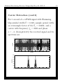
Johnson/Introducing Receiver Design/Apr-May 06: DAY 2
Phase-locked Loop (PLL)
To introduce a phase-locked loop, the most widely
known carrier recovery scheme, we present a
candidate cost function producing the PLL.
• Reconsider the output of the squarer and
narrow BPF, which is a scaled version of the
carrier x(kTs ) = g cos(4πf0 kTs + 2φ) where g
is s2avg /2 times the square of the product of
the channel and BPF gains at 2f0 and ψ is
the BPF phase (mod 2π) at 2f0 .
• Consider downconverting x(kTs ) with our
(unsynchronized) receiver oscillator’s output
and form
x(kTs ) cos(4πf0 kTs + 2θ + ψ)
≈ g cos(4πf0 kTs +2φ+ψ) cos(4πf0 kTs +2θ+ψ)
g
= {cos(2φ−2θ)+cos(8πf0 kTs +2φ+2θ+2ψ)}
2
35
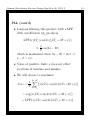
Johnson/Introducing Receiver Design/Apr-May 06: DAY 2
PLL (cont’d)
• Lowpass filtering this product with a LPF
with cutoff below 4f0 produces
LPF{x(kTs ) cos(4πf0 kTs + 2θ + ψ)}
g
≈ cos(2φ − 2θ)
2
which is maximized when 2φ − 2θ = 2nπ ⇒
φ − θ = nπ.
• Value of positive, finite g does not effect
locations of maxima and minima.
• We will choose to maximize
JP LL
k0 +P
1 X
{x(kTs ) cos(4πf0 kTs +2θ+ψ)}
=
P
k=k0
= avg{x(kTs ) cos(4πf0 kTs + 2θ + ψ)}
∼ LPF{x(kTs ) cos(4πf0 kTs + 2θ + ψ)}
36
Johnson/Introducing Receiver Design/Apr-May 06: DAY 2
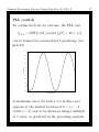
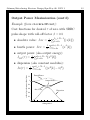
37
PLL (cont’d)
As a numerical test for extrema, the PLL cost
JP LL = LPF{x(kTs )cos(4πf0 kTs + 2θ + ψ)}
can be formed for various fixed θ producing (via
pllcrt)
0.5
0.4
0.3
0.2
Cost Jpll(θ)
0.1
0
−0.1
−0.2
−0.3
−0.4
−0.5
−3
−2
−1
0
Phase Estimates θ
1
2
3
A maximum (near 0.5 with g ≈ 1 in this case)
appears at the desired location of θ = φ = −1
(with ψ = 0) and at locations an integer multiple
of π away, as predicted in the preceding analysis.
Johnson/Introducing Receiver Design/Apr-May 06: DAY 2
38
PLL (cont’d)
Following a gradient ascent strategy for
maximization, compose
θ[k + 1] = θ[k]
∂
+µ̄ [avg{x(kTs ) cos(4πf0 kTs + 2θ + ψ)}]|θ=θ[k]
∂θ
With a small stepsize assuring (approximate)
commutability of differentiation and average
θ[k + 1] = θ[k]
∂
+µ̄ · avg{ [x(kTs ) cos(4πf0 kTs + 2θ + ψ)]|θ=θ[k] }
∂θ
where
∂
[x(kTs ) cos(4πf0 kTs + 2θ + ψ)]|θ=θ[k]
∂θ
= −2x(kTs ) sin(4πf0 kTs + 2θ[k] + ψ)
This produces
θ[k+1] = θ[k]−µLPF{x(kTs ) sin(4πf0 kTs +2θ[k]+ψ)}
Johnson/Introducing Receiver Design/Apr-May 06: DAY 2
39
PLL (cont’d)
PLL carrier recovery system:
rp(kTs)
2 ma
LPF
u[k]
sin(4pf0kTs 1 2u[k] 1 c)
,
2
where input rp is the processed received signal of
r(t)
X2
Squaring
nonlinearity
r 2(t)
BPF
rp(t) ~ cos(4pf0 t 1 2f 1 c)
Center frequency
at 2f0
and “normalizing” gain (2/s2avg ) has been
implicitly included in BPF (though any
substantial gain is acceptable) which has phase
shift ψ at frequency 2f0 .
When ψ is nonzero, it should be added in carrier
recovery system schematic after 2θ[k] term in the
oscillator.
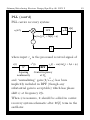
Johnson/Introducing Receiver Design/Apr-May 06: DAY 2
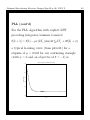
40
PLL (cont’d)
For the PLL algorithm with explicit LPF
preceding integrator/summer removed
θ[k + 1] = θ[k] − µx(kTs ) sin(4πf0 kTs + 2θ[k] + ψ)
a typical learning curve (from pllcrt) for a
stepsize of µ = 0.001 for our continuing example
(with ψ = 0 and an objective of θ = −1) is
Phase Tracking via the Phase Locked Loop
0.2
0
phase offset
−0.2
−0.4
−0.6
−0.8
−1
−1.2
0
0.2
0.4
0.6
0.8
1
time
1.2
1.4
1.6
1.8
2
Johnson/Introducing Receiver Design/Apr-May 06: DAY 2
Costas Loop
Now, we seek an algorithm not based on a
presumption of carrier extraction from the
received signal.
• Reconsider the received signal
r(kTs ) = s(kTs ) cos(2πf0 kTs + φ)
and form
2r(kTs ) cos(2πf0 kTs + θ)
= s(kTs )[cos(φ − θ) + cos(4πf0 kTs + φ + θ)]
• With a LPF cutoff below 2f0
LPF{2r(kTs ) cos(2πf0 kTs + θ)}
= v(kTs ) cos(φ − θ)
where v(kTs ) = LPF{s(kTs )}. If the cutoff
frequency of the LPF is above the bandwidth
of the baseband waveform s, then v is s.
41
Johnson/Introducing Receiver Design/Apr-May 06: DAY 2
Costas Loop (cont’d)
• As a cost function, consider
1
P
k0
X
{LPF[2r(kTs ) cos(2πf0 kTs +θ)]}2
k=k0 −(P −1)
≈ avg{v 2 (kTs ) cos2 (φ − θ)}
• Because the squared cosine term is fixed,
avg{v 2 (kTs ) cos2 (φ − θ)}
(1 + cos(2(φ − θ)))
= avg{v (kTs )}
2
and assuming that the average of v 2 is fixed,
this cost function will be maximized with a
value equal to the average of v 2 (which is
average value of {LPF[s]}2 ) at φ − θ = πn or
θ = φ + πn for all (positive and negative)
integers n.
2
42
Johnson/Introducing Receiver Design/Apr-May 06: DAY 2
43
Costas Loop (cont’d)
We can numerically check the extrema of a
normalized cost
PP
2
1
(LPF{2r(kT
)cos(2πf
kT
+
θ)})
s
0
s
JN C = P k=1 1 PP
2
(LPF{s(kT
)})
s
k=1
P
where r is the received signal for our continuing
example for various fixed θ producing (via ccrt)
1.4
1.2
Cost Jnc(θ)
1
0.8
0.6
0.4
0.2
0
−3
−2
−1
0
Phase Estimates θ
1
2
This normalized cost function matches
(1 + cos(2(φ − θ)))/2, as anticipated.
3
Johnson/Introducing Receiver Design/Apr-May 06: DAY 2
44
Costas Loop (cont’d)
Our next step in our algorithm creation strategy
is to interchange the averaging and differentiation
in the gradient ascent update
θ[k + 1] = θ[k] + µ̄
∂
[avg{(LPF{2r(kTs )
∂θ
2
·cos(2πf0 kTs + θ)}) }]|θ=θ[k]
With
LPF{2r(kTs )cos(2πf0 kTs +θ)} = v(kTs ) cos(φ−θ)
the update can be written as
∂ 2
θ[k+1] = θ[k]+µ̄·avg{ [v (kTs ) cos2 (φ−θ)]|θ=θ[k] }
∂θ
∂ cos(φ − θ)
)|θ=θ[k] }
∂θ
dy
d
and from dx
(cos(y)) = −(sin(y)) dx
we wish to
form
= θ[k]+µ·avg{v 2 (kTs )(cos(φ−θ)
θ[k + 1] = θ[k]
+µ · avg{v 2 (kTs ) cos(φ − θ[k]) sin(φ − θ[k])}
Johnson/Introducing Receiver Design/Apr-May 06: DAY 2
Costas Loop (cont’d)
Given
LPF{2r(kTs )cos(2πf0 kTs +θ)} = v(kTs ) cos(φ−θ)
to compose the update from measurable signals
we need to find a realizable expression for
v(kTs ) sin(φ − θ).
For a LPF with cutoff under 2f0 , defining
v = LPF{s} and using
sin(x) cos(y) = (1/2)[sin(x − y) + sin(x + y)] and
sin(−x) = − sin(x) produces
LPF{2r(kTs ) sin(2πf0 kTs + θ)}
= LPF{s(kTs ) cos(2πf0 kTs + φ) sin(2πf0 kTs + θ)}
= LPF{s(kTs )(sin(θ − φ) − sin(4πf0 kTs + φ + θ))}
= −v(kTs ) sin(φ − θ)
45
Johnson/Introducing Receiver Design/Apr-May 06: DAY 2
Costas Loop (cont’d)
Thus, a small stepsize gradient ascent algorithm
(for maximization of JC ) is
θ[k + 1] = θ[k]
−µ · avg[LPF{2r(kTs ) cos(2πf0 kTs + θ[k])}
·LPF{2r(kTs ) sin(2πf0 kTs + θ[k])}]
• The use of lowpass filtering in the update is
predicated on a presumption that the LPF
output is characterized by its asymptotic
response.
• This effectively presumes θ[k] remains fixed
for a sufficiently long time for this asymptotic
behavior to be achieved.
• We rely on a small stepsize µ to keep θ[k]
variations modest in the (relatively) short
time frame anticipated for LPF achievement
of asymptotic behavior.
46
Johnson/Introducing Receiver Design/Apr-May 06: DAY 2
47
Costas Loop (cont’d)
Schematic for Costas loop carrier phase recovery
with the “outer” averaging removed (which
presumes that the integrator/summer of the
update will provide sufficient averaging):
,
2cos(2pf0kTs 1 u[k])
LPF
u[k]
r(kTs)
2ma
LPF
,
2sin(2pf0kTs 1 u[k])
Johnson/Introducing Receiver Design/Apr-May 06: DAY 2
48
Costas Loop (cont’d)
A typical learning curve for this Costas loop
carrier phase recovery scheme (as shown in the
preceding schematic without explicit averaging in
the update) on our continuing example (with an
objective of −1) is (from ccrt with a stepsize of
µ = 0.001)
Phase Tracking via the Phase Locked Loop
0
−0.2
phase offset
−0.4
−0.6
−0.8
−1
−1.2
−1.4
0
0.2
0.4
0.6
0.8
1
time
1.2
1.4
1.6
1.8
2
Johnson/Introducing Receiver Design/Apr-May 06: DAY 2 LAB
1
Laboratory Exercises – Day 2
Introduction to Digital Communication Receiver Design
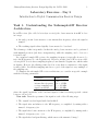
Task 1: Understanding the Subsampled-IF Receiver
Architecture
In an IF receiver (also called a heterodyne receiver), the downconversion from RF is done
in 2 steps:
• An analog circuit downconverts to some intermediate frequency, where the signal is
sampled.
• The resulting signal is then digitally downconverted to baseband.
The advantage of this 2-step method is that the analog downconversion can be performed
with minimal precision (and hence inexpensively), while the sampling can be done at a
reasonable rate.
In a standard sampled-IF receiver, the sampling frequency is typically chosen to be
twice the IF frequency (i.e. the Nyquist rate). However, another class of IF receivers called
subsampled IF receiver uses a sampling frequency lower than the Nyquist rate, which results
in aliasing. However, the aliasing is introduced in a way that reconstruction of the signal
is still possible. Recall that sampling introduces copies of the signal at every multiple of
the sampling rate.
To illustrate the subsampled IF receiver architecture, we consider an specific example
with the following parameters:
parameter
carrier frequency
intermediate frequency
receiver sampling rate
signal bandwidth
value
fRF = 1 GHz
fIF = 2 MHz
fs = 850 kHz
B = 100 kHz
where the signal bandwidth of the baseband signal is defined as having spectral content
between −B and +B.
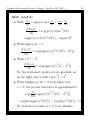
Your task: Draw the spectrum of the signal at each of the following steps
1. The original baseband signal with bandwidth B.
2. The signal after modulation to the RF frequency, accomplished by mixing with a
sinusoid of frequency fRF .
3. The signal after downconversion to the IF frequency, accomplished by mixing with a
sinusoid of frequency fRF − fIF .
4. The signal after bandpass filtering, which removes the unwanted “image”.
Johnson/Introducing Receiver Design/Apr-May 06: DAY 2 LAB
2
5. The signal after (sub)sampling at rate fs (Note: For this one, you only need to draw
the spectrum between −fs /2 and +fs /2).
If the next step were to perform downconversion of the signal to baseband, what frequency
would you choose for the sinusoid used in the downconversion?
In spite of the fact that subsampling introduces aliasing, is it still possible to recover
the original baseband signal? Or is the signal distorted?
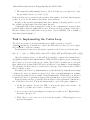
A subsampled-IF receiver is attractive because it can be implemented even more inexpensively than a standard sampled-IF receiver. However, there is one major drawback to
this use of this receiver architecture in the presence of noise (AWGN). Can you think of
what this drawback might be?
Task 2: Implementing the Costas Loop
The receiver you have been given currently uses a PLL for carrier recovery (in
/system code/Rx.m). Your task is to replace the PLL with a Costas loop, and compare
the performance of the two schemes.
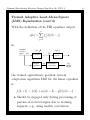
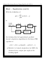
Recall from the lecture notes, the update equation for the Costas loop has the form
θ[k + 1] = θ[k] − µ · LPF {2r(kTs ) cos(2πf0 kTs + θ[k])} · LPF {2r(kTs ) sin(2πf0 kTs + θ[k])}
Since the existing receiver code has a PLL, it is useful to compare and contrast the two
algorithms in terms of their implementation. While the PLL requires a pre-processing step,
the Costas loop does not require pre-processing. The Costas loop makes use of a low pass
filter, which is not present in the PLL, and you will need to use remez to design this filter.
The schematic for the Costas loop on the next to last page of the lecture notes for DAY 2
may be helpful, as well.
In testing your Costas loop implementation, you should start by using the most benign
conditions (no noise, no channel, no phase noise). Once your implementation is working,
you should gradually add more realistic channel impairments. Additionally, you will need
to tune the Costas loop parameters (stepsize, filter parameters, etc) for best performance.
In the following exercises, you should check how the receiver performs in comparison to
the old PLL-based receiver. You should always include a plot of the phase estimate, θ.
1. Modify the channel, decrease the SNR, or increase the phase noise variance. In
general, do you find one receiver to be more robust?
2. Is one receiver better at tracking the variation due to phase noise? Explain this by
referring to the plot of θ.
3. What effect to you observe as you decrease the stepsize? What happens as you
increase the stepsize?
Johnson/Introducing Receiver Design/Apr-May 05: KLEIN’S RADIO
1
Transmitter/Receiver Code Description
Introduction to Digital Communication Receiver Design
Introduction
A transmitter and sampled-IF receiver have been implemented in Matlab, and this document describes the corresponding code. This operation of the receiver, including its chosen
parameters, are described in the latter half of the lecture notes for DAY 4 under the heading of “Putting It All Together: Receiver Design”. This receiver system will be used in
the lab assignments for Days 2-4 by focusing only on the specific segment described in the
associated lectures, while allowing us to judge the impact on overall system performance.
The block diagram in Fig. 1 shows the steps of generation of the transmitted signal, its
propagation through the channel, and the operations performed by the receiver. While
Binary
message
sequence b
we{23, 21, 1, 3}
Analog
upconversion
Carrier
specification
P(f)
Coding
Pulse
shaping
Transmitted
signal
Channel
Other FDM
Noise
users
1
1
Antenna
Analog
received
signal
Analog
conversion
to IF
Digital downconversion
to baseband
Pulse
matched
filter
Ts
Carrier
Input to the
synchronization
software
receiver
m
T
Downsampling
Timing
synchronization
Equalizer
Q(m)e{23, 21, 1, 3}
Decision
^
b
Decoding
Source and Reconstructed
error coding
message
frame synchronization
Figure 1: System Block Diagram
the blocks in this figure are quite general, design choices were made in the development
of this particular transmitter/receiver implementation. These design choices (i.e. which
algorithms have been selected) and the code to implement them will be described in the
following sections.
Matlab Files
A brief description of each of the functions used in the complete system is provided here.
You can find all of the files in the /system code directory. For a more detailed description
Johnson/Introducing Receiver Design/Apr-May 05: KLEIN’S RADIO
2
of the inputs and outputs for each of these functions, you can using the help command at
the Matlab prompt (e.g. by typing “help Tx”).
Main Files
Listings at the end of this code description document.
• main.m — This script is merely an example which shows how to set up the system
parameters, run the transmitter, run the receiver, and calculate the bit-error-rate.
• Tx.m — This function contains the transmitter, and introduces the impairments (e.g.
the channel, imperfect receiver frontend, etc.)
• Rx.m — This function decodes the received signal, and outputs the message.
• globalParams.m — This function contains the parameters for the system (e.g. sampling period, IF frequency, marker sequence, etc.)
Subroutine Files
These files are from Telecommunication Breakdown.
• letters2pam.m — This function converts an ASCII text sequence into 4-PAM symbols. Used by Tx.m.
• pam2letters.m — This function converts a sequence of 4-PAM symbols into an
ASCII text string. Used by Rx.m.
• quantalph.m — This function is effectively a minimum Euclidean distance detector,
or decision device. It accepts “soft” PAM symbols, and quantizes the input to the
nearest PAM symbol. Used by Rx.m.
• srrc.m — This function generates the impulse response for the square-root raisedcosing pulse shape. Used by both Tx.m and Rx.m.
• interpsinc.m — The function performs sinc interpolation, and is used for the baudtiming and downsampling in the receiver. Used by Rx.m.
Transmitter Details (Tx.m)
This section briefly describes each of the main components of the transmitter, and points
to their corresponding line numbers in the code. The components can also be found in the
block diagram in Fig. 1. Note that, in addition to the transmitter, Tx.m also includes the
channel and receiver frontend blocks.
Johnson/Introducing Receiver Design/Apr-May 05: KLEIN’S RADIO
3
• Calculate Intermediate Variables (lines 19-29) — This part calculates intermediate variables which are used in the transmitter, including the upsampling/downsampling
ratios and the phase noise random process.
• Generation of 4-PAM sequence (lines 30-32) — This part encodes the ASCII test
message into 4-PAM signals (using letters2pam), and inserts the header and marker
sequences. The result is a serial stream of 4-PAM symbols stored in the variable
called s.
• Pulse Shaping (lines 33-35) — This part performs upsampling of the 4-PAM signal
and then filters the signal with the pulse shape obtained from srrc. The result is
stored in the variable x.
• Analog Upconversion (lines 36-39) — This part modulates the signal up to the
carrier frequency, and includes the effect of phase noise. The result is stored in x rf.
• Channel (lines 40-42) — This part convolves the upconverted signal with the channel, storing the result in the variable x2.
• Noise (lines 43-47) — This part adds the additive white Gaussian noise of specified
SNR.
• Analog Conversion from RF to IF (lines 48-52) — This part acts as the frontend
of the receiver, and performs analog conversion of the RF signal down to IF. While
the RF signal in reality would be analog, our computer simulation uses a digital
representation throughout; thus, the sampled-IF receiver is obtained from the RF
signal by simple downsampling. The result is the digital signal which gets passed
into Rx.m.
Receiver Details (Rx.m)
Similar to the previous section, this section briefly describes each of the main components
of the receiver, and points to their corresponding line numbers in the code. Most of the
components can also be found in the block diagram in Fig. 1.
• Calculate Intermediate Variables (lines 18-25, 52-72) — This part calculates intermediate variables which are used in the receiver. This includes calculation of the
effective carrier frequency and image frequency, memory allocation, variable allocation, and size determination.
• Digital Downconversion via PLL (lines 26-34, 74-82) — This part implements
the downconversion which is accomplished in the current receiver with a PLL. The
procedure consists of several sub-steps:
– Parameter Initialization and Bandpass Filter Design (lines 26-34)
– PLL Pre-processing (lines 74-76)
– PLL Adaptation (lines 77-79)
Johnson/Introducing Receiver Design/Apr-May 05: KLEIN’S RADIO
4
– Mixing (lines 80-82)
Recall that the equation for PLL adaptation has the form
θ[k + 1] = θ[k] − µx(kTs ) sin (4πf0 kTs + θ[k] + ψ)
which appears in line 78. The carrier phase estimate is stored in the variable theta
while the downconverted signal is stored in the variable x down.
• Pulse Matched Filter (lines 48-51, 83-85) — This part performs filtering of the
signal with the square-root raised-cosine filter. The filtered signal is stored in the
variable x bb.
• Downsampling/Timing Sync via Output Power (OP) Method (lines 35-38,
89-96) — This part performs the downsampling and timing synchronization using
the method of output power maximization. The procedure makes several calls to the
interpsinc function, and consists of several sub-steps:
– Parameter Initialization (lines 35-38)
– Get current interpolated value (line 90)
– Calculate approximate derivative (lines 91-93)
– Algorithm Adaptation (line 94)
Recall the equation for the output-power-maximizing baud-timing adaptation algorithm has the form
"
!
kT
kT
τ [k + 1] = τ [k] + µx[k] x
+ τ [k] + δ − x
+ τ [k] − δ
M
M
!#
which is seen in lines 91-94. The Matlab variable tau stores the timing offset, tnow
stores the current position, and x sampled stores the downsampled signal after timing
recovery.
• Correlation (lines 97-102) — Always running, this part calculates the correlation of
the downsampled signal with the known header sequence.
• Header Search (lines 39-41, 104-110) — This part searches for the header, by
comparing the correlation value with a threshold.
• Equalization with Adaptation via LMS (lines 111-124) — This part performs
equalization of the signal, which includes adaptation of the equalizer coefficient during
training periods (see paragraph below about different operating modes of receiver).
Equalization consists of two sub-steps
– Adapt equalizer using LMS (lines 111-121)
– Generate equalizer output (lines 121-124)
Johnson/Introducing Receiver Design/Apr-May 05: KLEIN’S RADIO
5
Recall the equation for the LMS algorithm which has the form
fi [k + 1] = fi [k] + µ (s[k − δ] − y[k]) r[k − i]
and is seen in lines 114-115. The Matlab variable f stores the equalizer coefficients,
and eqOut stores the output of the equalizer.
• Decision Device, Frame Sync, and Message Decoding (lines 125-129) — This
part quantizes the equalizer output using quantalph, resulting in a stream of 4-PAM
symbol estimates stored in the variable dec. With knowledge of the start of the
header sequence from the previous stage, frame synchronization is performed, after
which the decisions pass into the decoder (i.e. pam2letters), the output of which is
stored in the variable decoded msg.
There are some other details of the receiver which are worth noting. The receiver consists
of two main loops and their corresponding counters
1. IFsampleIdx — Each time this loop counter is incremented, the receiver has received
a new IF sample at the receiver frontend.
2. BBsampleIdx — This loop counter is incremented every time a new baseband sample
is output from the baud-timing device.
Also, the receiver operates in 3 distinct modes:
1. HEADER SEARCH MODE — In this mode, the receiver is running its correlator to search
for the header sequence.
2. TRAINING MODE — In this mode, the receiver thinks that it is receiving training data,
and so it is training the equalizer using the LMS algorithm.
3. DATA MODE — In this mode, the receiver has completed training, and believes that it
is receiving data.
The receiver starts in HEADER SEARCH MODE. Once the header is found, it switches to
TRAINING MODE, and when the training is complete it switches to DATA MODE. Once the
data transmission is complete (based on the length of the data sequence specified in the
system parameters), the receiver then returns to HEADER SEARCH MODE and repeats.
Listings
main.m
1
2
3
% Example script that demonstrates how to call transmitter and rece
iver
% code.
Johnson/Introducing Receiver Design/Apr-May 05: KLEIN’S RADIO
4
5
6
7
8
9
10
11
12
13
14
15
16
17
18
19
20
21
22
23
24
25
26
27
28
29
30
31
32
33
34
% written by A. Klein 26-Oct-2005
% call script to get global simulation parameters (i.e. carrier fre
q, baud rate, training data, etc)
globalParams
% initialize random seed for repeatability (helps for debugging) -randn(’state’,0);
rand(’state’,0);
% set channel, SNR, phase noise,
c = [1 -0.4 0.2];
%
SNR = 18;
%
er) sampled signal
phase_noise_variance = 1e-6;
%
process
%
%
%
%
and message to be sent ----------channel (T-spaced)
signal-to-noise ratio (dB) of (und
variance of underlying phase noise
(uncomment the following lines for the most benign conditions)
c = [1 0 0];
% no ISI
SNR = Inf;
% no noise
phase_noise_variance = 0;
% perfect oscillators
m=[’This is the first frame which you probably shouldn’’t able to d
ecode perfectly unless you "cheat" and’
’give your receiver the initial points. Now we’’re into the second
frame. You might be able to decod’
’e this one, and now the third, error-free. . . But if you didn’’t,
then don’’t worry yet. The only fr’
’ames you are required to decode during the actual testing are thos
e past the fifth frame. So you’’re’
’still okay. We’’re getting close to the end of the 5th frame, so
your receiver better start working.’
’Congratulations! If you can see this then you’’re receiver has su
ccessfully decoded the fifth frame.’
’You might want to re-test your receiver by using different initial
parameters, and different stepsiz’
’es to see what the effect is. It’’s probably help to plot the tim
e history of the adaptive parameter’
’elements, too, so you can see if they’’re taking too long to conve
rge, if they seem unstable, etc. A’
’nd now some more Nirvana lyrics: With the lights out it’’s less da
ngerous Here we are now Entertain u’
’s I feel stupid and contagious Here we are now Entertain us A mula
tto An albino A mosquito My Libido’
’And I forget Just what it takes And yet I guess it makes me smile
6
Johnson/Introducing Receiver Design/Apr-May 05: KLEIN’S RADIO
35
36
37
38
39
40
41
42
43
44
45
46
I found it hard Its hard to find. ’
’Well, if your receiver has made it this far with no errors, and pe
rforms error-free even when you ch’
’ange the initial parameter values, then it’’s time to move on to t
he "medium" test vector. Good luck’];
% call transmitter -----------------------------------------------[r, s]=Tx(m, c, SNR, phase_noise_variance);
m=m’; m=m(:)’;
% call receiver --------------------------------------------------[decoded_msg y]=Rx(r);
% call code to calculate BER ----------------------------------BERcalc
Tx.m
1
2
3
4
5
6
7
8
9
10
11
12
13
14
15
16
17
18
19
20
21
22
23
24
25
26
27
function [r, s]=Tx(m, c, SNR, phase_noise_variance)
% function [r, s]=Tx(m, c, SNR, phase_noise_variance)
%
% Inputs:
%
m -- text message to be sent
%
c -- channel (T-spaced)
%
SNR -- signal to noise ratio
% phase_noise_variance -- variance of phase noise added to signal
%
% Outputs:
%
r -- received signal (at IF)
%
s -- transmitted symbols (for calculating SER)
% written by A. Klein 26-Oct-2005
global srrcLength marker training f_s T_t f_if rolloff dataLength
% determine suitable oversampling/downsampling factor
[M N]=rat(f_s*T_t);
M_scale=ceil((2*T_t*f_if+1+rolloff)/M);
M=M*M_scale;
N=N*M_scale;
% get dimensions
lines_of_text=size(m,1);
frame_length=(dataLength+(length([marker; training])));
7
Johnson/Introducing Receiver Design/Apr-May 05: KLEIN’S RADIO
28
29
30
31
32
33
34
35
36
37
38
39
40
41
42
43
44
45
46
47
48
49
50
51
52
53
54
char_str_length=frame_length*lines_of_text;
% insert training & header, and generate 4-PAM source vector
s=reshape([repmat([marker; training]’,lines_of_text,1) reshape(lett
ers2pam(reshape(m’,lines_of_text*dataLength/4,1)),dataLength,lines_
of_text)’]’,lines_of_text*(dataLength+(length([marker; training])))
,1);
% generate pulse-shaped signal
x=conv(srrc(srrcLength,rolloff,M,0)’,upsample(s,M));
% mix signal to RF (analog upconversion)
p_noise=cumsum(randn(size(x))*sqrt(phase_noise_variance/N)); % gene
rate phase noise process
x_rf=x.*cos(2*pi*f_if*[1:length(x)]’*T_t/M+p_noise);
% pass through BP channel
x2=conv(x_rf,upsample(c,M));
% add channel noise of appropriate SNR
x2_size=size(x2);
x2_nrm=sqrt(x2(srrcLength*M+1:x2_size(1)-srrcLength*M)’*x2(srrcLeng
th*M+1:x2_size(1)-srrcLength*M)/x2_size(1));
x_r=x2+randn(size(x2))*10^(-SNR/20)*x2_nrm;
% perform analog conversion to IF, and do AGC
r=x_r(N:N:end);
r_nrm=r’*r/length(r);
r=r/sqrt(r_nrm);
% add some zeros to front and back
r=[zeros(floor(rand*10*M),1); r; zeros(10*M,1)];
Rx.m
1
2
3
4
5
6
7
8
9
10
function [decoded_msg, eqOut]=Rx(r)
% function [decoded_msg, eqOut]=Rx(r)
%
% Inputs:
%
r -- received signal (at IF)
%
% Outputs:
%
decoded_msg -- received signal (at IF)
%
eqOut
-- output of equalizer
8
Johnson/Introducing Receiver Design/Apr-May 05: KLEIN’S RADIO
11
12
13
14
15
16
17
18
19
20
21
22
23
24
25
26
27
28
29
30
31
32
33
34
35
36
37
38
39
40
41
42
43
44
45
46
47
48
49
50
51
% written by A. Klein 26-Oct-2005
global srrcLength marker training f_s T_t f_if rolloff dataLength
globalParams
% calculate new effective carrier frequency, and the image which wi
ll appear at 2f_c (and may get aliased)
f_c=f_if-fix(f_if/f_s)*f_s;
f_image=abs(mod(2*f_c+f_s/2,f_s)-f_s/2);
% calculate sizes ----------------------------markerLength=length(marker);
trainingLength=length(training);
% PLL parameters & BPF filter design -----------------------------bpf_ctr=f_image/f_s*2;
% set center frequency of BPF to 2f
BPFfilterOrder=500;
% should be an even number
ff=[0 bpf_ctr+[-0.006 -0.003 0.003 0.006] 1]; % BPF trans. band
fa=[0 0 1 1 0 0];
% values at transition regions
h=remez(BPFfilterOrder,ff,fa)’;
% design filter
phaseBPF=angle(exp(-1j*[0:length(h)-1]*pi*bpf_ctr)*h); % calculate
phase introduced by BPF
mu_PLL=0.001;
% stepsize for first PLL loop
% baud timing (OP) parameters -----------------------mu_timing=0.1;
% algorithm stepsize
delta=0.1;
% time for derivative
% correlation (i.e. header search) parameters --------correlThresh=6500;
% threshold for
determining whether we’ve received the header sequence
% equalizer parameters --------------------------eqLength=8;
% equalizer length
mu_eq_lms=0.005;
% trained LMS stepsize
eqDelay=3;
% desired delay (for LMS)
f=zeros(eqLength,1); f(eqDelay+1)=1; % equalizer initialization (m
ust have correct length)
% design SRRC (matched) filter --------------------------srrcFlt=srrc(srrcLength,rolloff,f_s*T_t,0)’;
srrcFltLength=length(srrcFlt);
9
Johnson/Introducing Receiver Design/Apr-May 05: KLEIN’S RADIO
52
53
54
55
56
57
58
59
60
61
62
63
64
65
66
67
68
69
70
71
72
73
74
75
76
77
78
79
80
81
82
83
84
85
86
% setup constants for each of the three operating modes-----------HEADER_SEARCH_MODE=1;
TRAINING_MODE=2;
DATA_MODE=3;
operationMode=HEADER_SEARCH_MODE; % we start in HEADER_SEARCH_MODE
% allocate memory and initialize variables --------------theta=zeros(length(r),1);
% stores outputs of PLL
x_down=zeros(length(r),1);
% stores downconverted signal (prematched filter)
x_bb=zeros(length(r),1);
% stores baseband signal (post-matc
hed filter)
x_sampled=zeros(ceil(length(r)/T_t/f_s),1); % stores sampled signa
l (post timing recovery)
Corr=zeros(ceil(length(r)/T_t/f_s),1);
% stores correlation v
alues (for header search)
tau=zeros(ceil(length(r)/T_t/f_s),1);
% stores timing recovery (
only used for plotting)
eqOut=zeros(ceil(length(r)/T_t/f_s),1); % stores output of equalizr
e_lms=zeros(ceil(length(r)/T_t/f_s),1);
% stores LMS error
dec=zeros(ceil(length(r)/T_t/f_s),1);
% stores PAM-4 decisions
packetIndex=0;
% packet counter
tnow=2*(srrcLength-2)*T_t*f_s;
% starting location for timing
BBsampleIdx=0;
% intialize baseband sample counter
start=BPFfilterOrder+1;
% outer loop starting point
for IFsampleIdx=start:length(r);
% pre-process signal for PLL
r2(IFsampleIdx)=h’*r(IFsampleIdx:-1:IFsampleIdx-BPFfilterOrder)
.^2;
% adapt PLL
theta(IFsampleIdx+1)=theta(IFsampleIdx)-mu_PLL*r2(IFsampleIdx)*
sin(4*pi*f_c*IFsampleIdx/f_s+2*theta(IFsampleIdx)+phaseBPF);
% perform downconversion
x_down(IFsampleIdx)=r(IFsampleIdx)*cos(2*pi*f_c*IFsampleIdx/f_s
+theta(IFsampleIdx));
% perform matched filtering
x_bb(IFsampleIdx)=srrcFlt’*x_down(IFsampleIdx:-1:IFsampleIdx-sr
rcFltLength+1);
while tnow<IFsampleIdx-2*srrcLength*T_t*f_s+2
% do we have a new baseband sample?
10
Johnson/Introducing Receiver Design/Apr-May 05: KLEIN’S RADIO
87
88
89
90
91
92
93
94
95
96
97
98
99
100
101
102
103
104
105
106
107
108
109
111
BBsampleIdx=BBsampleIdx+1;
% ok, we’re at next baseband sample, so increment
% perform timing recovery (OP)
x_sampled(BBsampleIdx)=interpsinc(x_bb,tnow+tau(BBsampleIdx
),srrcLength);
% interpolated value at tnow+tau
x_deltap=interpsinc(x_bb,tnow+tau(BBsampleIdx)+delta,srrcLe
ngth);
% get value to the right
x_deltam=interpsinc(x_bb,tnow+tau(BBsampleIdx)-delta,srrcLe
ngth);
% get value to the left
dx=x_deltap-x_deltam;
% calculate numerical derivative
tau(BBsampleIdx+1)=tau(BBsampleIdx)+mu_timing*dx*x_sampled(
BBsampleIdx);
% alg update: OP
tnow=tnow+T_t*f_s;
% update current position
% run correlator, matched to marker sequence
if (BBsampleIdx>eqDelay+markerLength-1)
% need to skip t
he first few sample until we have enough to fill correlator
corInputSignal=x_sampled(BBsampleIdx-markerLength+1-eqD
elay:BBsampleIdx-eqDelay);
% extract portion of signal used f
or correlation
Corr(BBsampleIdx)=(marker’*corInputSignal)^2;
% calculate correlation
end
switch operationMode
case HEADER_SEARCH_MODE
% if we haven’t already fou
nd marker, look for it...
if Corr(BBsampleIdx)>correlThresh
% has cor
relation exceeded threshold?
operationMode=TRAINING_MODE;
% yep, so switch to training mode
trainingIndex=1;
% reset to trainingIndex to first sample of training data
packetIndex=packetIndex+1;
% increment packet counter
end 110
case TRAINING_MODE % if we’re in equalizer training mod
e, train the LMS equalizer
112
rr=x_sampled(BBsampleIdx:-1:BBsampleIdx-eqLength+1)
;
% extract "regressor" vector of receive
d signal
11
Johnson/Introducing Receiver Design/Apr-May 05: KLEIN’S RADIO
113
eqOut(BBsampleIdx)=f’*rr;
% equalizer output
114
e_lms(BBsampleIdx)=training(trainingIndex)-eqOut(BB
sampleIdx);
% calculate LMS error term
115
f=f+mu_eq_lms*e_lms(BBsampleIdx)*rr;
% update equalizer coefficients
116
trainingIndex=trainingIndex+1;
% increment training index location
117
if trainingIndex>trainingLength
% are we done training?
118
operationMode=DATA_MODE;
% yep, switch to data mode
119
symbolIndex=1;
% and re-init symbol counter to 1
120
end
121
122
case DATA_MODE
% we’re into data portion of the pack
et -- equalizer, and save data
123
rr=x_sampled(BBsampleIdx:-1:BBsampleIdx-eqLength+1)
;
% extract "regressor" vector of receive
d signal
124
eqOut(BBsampleIdx)=f’*rr;
% equalizer output
125
dec(symbolIndex)=quantalph(eqOut(BBsampleIdx),[-3 1 1 3]);
% make decisions
126
127
if mod(symbolIndex,4)==0
% if we’ve completed a w
hole letter (i.e. 4 PAM symbols), convert PAM symbols to letters
128
decoded_msg(packetIndex,symbolIndex/4)=pam2lett
ers(dec(symbolIndex-3:symbolIndex)’); % re-assemble text message
129
end
130
symbolIndex=symbolIndex+1;
% increment training index location
131
if symbolIndex>dataLength % are we done with data
yet?
132
operationMode=HEADER_SEARCH_MODE; % yep, switc
h back to header search mode
133
end
134
end
135
end
12
Johnson/Introducing Receiver Design/Apr-May 05: KLEIN’S RADIO
136
137
138
139
140
141
142
143
144
145
146
147
148
149
150
151
152
153
154
155
156
157
158
159
160
161
162
163
164
165
166
167
168
169
end
% plot results ---------------------------------------------------figure(1);
plot(theta)
title(’carrier phase estimate’)
ylabel(’theta’)
xlabel(’time’)
figure(2)
plot(tau)
title(’timing offset estimates’)
ylabel(’tau’)
xlabel(’time’)
figure(3)
plot(Corr)
hold on
plot([1 length(Corr)],[correlThresh correlThresh],’:’) % plot thre
shold
title(’correlator output (for finding start of training)’)
xlabel(’time’)
ylabel(’correlation value’)
figure(4)
plot(eqOut,’b.’)
% plot constellation diagram
title(’constellation diagram (equalizer output)’);
ylabel(’estimated symbol values’)
xlabel(’time’)
figure(5)
plot(e_lms)
title(’error at equalizer output (during training)’)
ylabel(’e_lms’)
xlabel(’time’)
globalParams.m
1
2
3
4
5
6
global srrcLength marker training f_s T_t f_if rolloff dataLength
srrcLength=4;
% truncated srrc length (divided by 2)
marker=letters2pam(’0’)’; % marker sequence
training=letters2pam(’Oh well whatever Nevermind’)’; % training se
quence
f_s=850e3;
% sampling frequency (Hz)
13
Johnson/Introducing Receiver Design/Apr-May 05: KLEIN’S RADIO
7
8
9
10
T_t=6.4e-6;
f_if=2e6;
rolloff=0.3;
dataLength=400;
%
%
%
%
symbol period (seconds)
intermediate frequency (Hz)
srrc rolloff factor
number of PAM symbols per data frame
14
Johnson/Introducing Receiver Design/Apr-May 06: DAY 3
DAY 3
• Pulse Shaping and Receive Filtering
• Baud Timing for Clock Recovery
1
Johnson/Introducing Receiver Design/Apr-May 06: DAY 3
PULSE SHAPING AND RECEIVE
FILTERING
? Pulse and Pulse Amplitude Modulated
Message Spectrum
? Eye Diagram
? Nyquist Pulses
? Matched Filtering
? Matched, Nyquist Transmit and Receive
Filter Combination
2
Johnson/Introducing Receiver Design/Apr-May 06: DAY 3
3
Pulse Shaping and Receive Filtering
Binary
message
sequence b
we{23, 21, 1, 3}
Analog
upconversion
Carrier
specification
P(f)
Coding
Pulse
shaping
Transmitted
signal
Channel
Other FDM
Noise
users
1
1
Antenna
Analog
received
signal
Analog
conversion
to IF
Digital downconversion
to baseband
Pulse
matched
filter
Ts
Carrier
Input to the
synchronization
software
receiver
T
Downsampling
Q(m)e{23, 21, 1, 3}
m
Equalizer
Decision
^
b
Decoding
Source and Reconstructed
error coding
message
frame synchronization
Timing
synchronization
We will focus on the situation where up and
downconversion have been flawlessly performed
and the effect of transmission from baseband
PAM message waveform to received signal is
presumed described by a linear transfer function
and the addition of interferers, in particular
spectrally flat broadband noise.
Message
w(kT)«{23, 21, 1, 3}
Noise
Interferers n(t)
x(t)
g(t)
Pulse
shaping
p(t)
P(f)
Channel
hc(t)
Hc(f)
1
y(t)
1
Receive
filter
hR(t)
HR(f)
Reconstructed
message
m(kT 2 d)i«{23, 21, 1, 3}
Decision
Johnson/Introducing Receiver Design/Apr-May 06: DAY 3
Pulse and pulse amplitude modulated
(PAM) message spectrum
Message
w(kT)«{23, 21, 1, 3}
Noise
Interferers n(t)
x(t)
g(t)
Pulse
shaping
p(t)
P(f)
Channel
1
y(t)
1
Receive
filter
Reconstructed
message
m(kT 2 d)i«{23, 21, 1, 3}
Decision
hR(t)
HR(f)
hc(t)
Hc(f)
The spectral footprint of a baseband PAM signal is
no wider than that of the pulse shape.
• Compose the analog pulse train entering the
pulse shaping filter as
X
wa (t) =
w(kT )δ(t − kT )
k
which is w(kT ) for t = kT and 0 for t 6= kT
• Pulse shaping filter output
x(t) = wa (t) ∗ p(t) ⇒ X(f ) = Wa (f )P (f )
• X(f ) cannot be nonzero at frequencies where
P (f ) is zero.
4
Johnson/Introducing Receiver Design/Apr-May 06: DAY 3
5
Pulse ... message spectrum (cont’d)
One-symbol wide Hamming blip pulse shape
(with 10 samples per symbol) and frequency
response (using freqz in pulsespec)
1
Pulse shape
0.8
0.6
0.4
0.2
0
0
0.1
0.2
0.3
0.4
0.5
Sample periods
0.6
0.7
0.8
0.9
Spectrum of the pulse shape
(a)
102
100
1022
1024
0
0.1
0.2
0.3
0.4
0.5
0.6
Normalized frequency
(b)
0.7
0.8
0.9
1
Johnson/Introducing Receiver Design/Apr-May 06: DAY 3
6
Pulse ... message spectrum (cont’d)
Spectrally flat 4-PAM symbol sequence triggering
baud-spaced 10-times oversampled Hamming blip
pulse shape as (baseband) output of pulse
shaping filter
Output of pulse
shaping filter
3
2
1
0
21
22
23
0
5
10
15
20
25
Symbols
Spectrum of the output
104
102
100
1022
1024
0
0.1
0.2
0.3
0.4
0.5
0.6
0.7
0.8
0.9
1
Normalized frequency
Message signal spectrum has scalloped contours
of Hamming blip pulse frequency response.
Johnson/Introducing Receiver Design/Apr-May 06: DAY 3
Eye Diagram
Eye diagram is a popular robustness evaluation
tool.
For 4-PAM, single-baud-wide Hamming blip with
additive broadband channel noise, retriggering
oscilloscope after every 2 baud intervals produces
Optimum sampling times
Sensitivity to
timing error
3
Distortion
at zero
crossings
2
1
0
21
22
23
Noise
margin
The "eye"
kT
(k 1 1)T
Observe illustrative vertical (amplitude) and
horizontal (timing) margins for correct decision at
sample times.
7
Johnson/Introducing Receiver Design/Apr-May 06: DAY 3
8
Eye Diagram (cont’d)
Consider 20-symbol wide, 10 times oversampled,
truncated, sinc pulse (sin(πt/T )/(πt/T )) with
zero-crossings at kT for k = 1, 2, ..., 10 for 4-PAM
symbol sequence (from spsex)
Using a sinc pulse shape
0.6
0.4
0.2
0
−0.2
−10
−8
−6
−4
−2
0
2
pulse shaped data sequence
4
6
8
10
4
2
0
−2
−4
0
5
10
15
20
25
symbol number
4
2
0
−2
−4
0
5
10
15
20
25
3−baud (and 30−sample) wide eye diagram (symbol times: indices 10, 20, and 30)
A multi-baud-wide pulse shape, but no ISI!
30
Johnson/Introducing Receiver Design/Apr-May 06: DAY 3
Nyquist Pulses
The impulse response of a Nyquist pulse creating
no ISI at other sample times is zero at those
instants and nonzero only at the one particular
sample time.
• The impulse response p(t) is a Nyquist pulse
for a T -spaced symbol sequence if there exists
a τ such that

 c, k = 0
p(t)|t=kT +τ =
 0, k 6= 0
• Rectangular pulse:

 1, 0 ≤ t < T
pR =
 0, otherwise
Rectangle is Nyquist pulse for almost any
sampler timing.
9
Johnson/Introducing Receiver Design/Apr-May 06: DAY 3
Nyquist Pulses (cont’d)
• Sinc pulse:
pS (t) =
sin πf0 t
πf0 t
where f0 = 1/T .
Sinc is Nyquist pulse because pS (0) = 1
and pS (kT ) = sin(πk)
= 0.
πk
Sinc envelope decays at 1/t.
• Raised-cosine pulse:
sin(2πf0 t)
cos(2πf∆ t)
pRC (t) = 2f0
2πf0 t
1 − (4f∆ t)2
with roll-off factor β = f∆ /f0 .
Raised-cosine is Nyquist pulse for
T = 1/2f0 because pRC has a sinc factor
sin(πk)/πk which is zero for all nonzero
integers k.
Raised-cosine envelope decays at 1/|t3 |.
As β → 0, raised-cosine → sinc.
10
Johnson/Introducing Receiver Design/Apr-May 06: DAY 3
Nyquist Pulses (cont’d)
• Raised-cosine pulse (cont’d):
Fourier transform


|f | < f1

 1,
1+cos(α)
PRC (f ) =
, f1 < |f | < B
2



0,
|f | > B
where
B is the absolute bandwidth,
f0 is the 6db bandwidth,
f∆ = B − f0 ,
f1 = f0 − f∆ , and
1)
α = π(|f2f|−f
∆
11
Johnson/Introducing Receiver Design/Apr-May 06: DAY 3
12
Nyquist Pulses (cont’d)
• Raised-cosine pulse (cont’d):
Time and Frequency Plots:
1
b51
0.5
b50
0
b 5 0.5
20.5
23T
22T
2T
0
T
b50
1
b 5 0.5
b51
0
0
f0/2
f0
3f0/2
2f0
2T
3T
Johnson/Introducing Receiver Design/Apr-May 06: DAY 3
Matched Filter
Suppose the channel simply adds broadband noise
n(t). The symbol to reconstructed downsample
system is described by
n(t)
m(kT )
1
Pulse
shaping
g(t)
Downsample
v(t)
P(f )
HR(f )
Pulse
shaping
Receive
filter
Downsample
w(kT )
w(t)
HR(f )
Receive
filter
m(kT )
HR(f )
Receive
filter
n(t)
y(kT )
y(t)
g(t)
P(f )
v(kT )
1
y(kT )
Downsample
so y(t) = v(t) + w(t) = hR (t) ∗ g(t) + hR (t) ∗ n(t).
• Our objective is to choose hR (t) to maximize
the power of the signal v(t) at a specific time
t = τ , i.e. v 2 (τ ), relative to the total power of
w(t) where the power spectral density of n(t)
is a constant η over all frequencies.
13
Johnson/Introducing Receiver Design/Apr-May 06: DAY 3
Matched Filter (cont’d)
With spectrally flat channel noise the
SNR-maximizing receive filter impulse response is
the time-reversal of that of the pulse shape.
• Example:
Minimum τ for causality of matched filter is
pulse width for pulse initiated at t = 0.
• Note: Minimum-delay matched filter is same
as pulse if pulse is causal and even symmetric.
14
Johnson/Introducing Receiver Design/Apr-May 06: DAY 3
Matched Nyquist Transmit and Receive
Filter Combinations
A preferred receive filter impulse response (in the
absence of channel ISI but with broadband channel
noise) (i) will match the reversed impulse
response of the transmitter pulse shape and (ii)
when convolved with the transmitter pulse shape
will form a Nyquist pulse.
• Want convolution of candidate pulse shape
g(t) and its matched filter g(t − τ ) to equal
even symmetric Nyquist pulse p(t).
• Since convolution of two even symmetric
pulse shapes is even symmetric, presume g(t)
is even symmetric, so with particular τ ,
g(t) = g(τ − t).
• Objective becomes
p(t) = g(t) ∗ g(t) ⇒ P (f ) = G2 (f )
15
Johnson/Introducing Receiver Design/Apr-May 06: DAY 3
16
Matched ... Combinations (cont’d)
• So, choose
p
p
−1
G(f ) = P (f ) ⇒ g(t) = F { P (f )}
• For example, consider the square-root raised
cosine (SRRC)

sin(π(1−α)t/T )+(4αt/T )cos(π(1+α)t/T )

√1

(πt/T )(1−(4αt/T )2 )

T



T

for
t
=
6
0,
t
=
6
±

4α

v(t) =









√1 (1 − α + (4α/π))
T
π
2
√α
1 + π sin 4α
2T
T
for t = ± 4α
for t = 0
+ 1−
2
π
cos
π
4α
which has a magnitude spectrum the square
of which equals the magnitude spectrum of a
raised cosine.
• The square root raised cosine is the most
commonly used pulse in bandwidth
constrained communication systems.
Johnson/Introducing Receiver Design/Apr-May 06: DAY 3
BAUD TIMING FOR CLOCK
RECOVERY
? A Baud-Timing Example
? Output Power Maximization
17
Johnson/Introducing Receiver Design/Apr-May 06: DAY 3
18
Baud-Timing
• Consider the situation where the up and
down conversion is done perfectly, so we need
only consider a baseband model of the
communication system.
h(t) 5 gR(t)*c(t)*gT(t)
gT(t)
s[i]
Transmit
Filter
gR(t)
c(t)
Channel
1
Receive x(t)
filter
Sampler
x(kT/M 1 t)
w(t)
• We are to select τ in
x[k] = x( kT
M + τ)
=
∞
X
!
s[i]h(t − iT ) + w(t) ∗ gR (t) |t= kT +τ
i=−∞
with
h(t) = gT (t) ∗ c(t) ∗ gR (t)
M
Johnson/Introducing Receiver Design/Apr-May 06: DAY 3
Baud-Timing (cont’d)
Three possible implementation configurations
Sampler
ASP
DSP
,
(a)
Sampler
ASP
DSP
,
(b)
Sampler
ASP
DSP
,
(c)
We favor the last with its free-running sampler
and fine tuning of the baud-timing done in the
receiver DSP.
19
Johnson/Introducing Receiver Design/Apr-May 06: DAY 3
A Baud-Timing Example
We will analyze the special case for
h(t) 5 gR(t)*c(t)*gT(t)
gT(t)
s[i]
gR(t)
c(t)
Transmit
Filter
Channel
Sampler
x(kT/M 1 t)
Receive x(t)
filter
1
w(t)
when
• the noise w is absent and
• the analog pulse-shaping filter, the channel
transfer function, and the receive filter
combine into an impulse response that is a
triangle spanning two symbol intervals.
h(t)
1.0
0 t0
T T 1 t0
Time t
2T
20
Johnson/Introducing Receiver Design/Apr-May 06: DAY 3
A Baud-Timing Example (cont’d)
• With perfect baud-timing (τ = 0)
baud-space-sampled (M = 1) combined
analog pulse/channel/receive filter impulse
response shape is a Nyquist pulse

 1, k = 1
h(kT ) =
 0, k 6= 1
• In general, without perfect baud-timing the
sampler output is a weighted combination of
several source symbol values
X
x[k] =
s[i]h(t − iT )
i
• Consider three cases:
τ =0
τ >0
τ <0
t=kT +τ
21
Johnson/Introducing Receiver Design/Apr-May 06: DAY 3
A Baud-Timing Example (cont’d)
• τ =0
Only one nonzero point in sampled
impulse response
Sampled impulse response
h(t − iT )|t=kT +τ
= h(kT + τ − iT )
= h((k − i)T + τ )
= h((k − i)T )



 1, k − i = 1
=
⇒ i=k−1



0, otherwise
x[k] = s[k − 1], system is pure delay, and
sampler is synchronized with transmitter
pulse.
22
Johnson/Introducing Receiver Design/Apr-May 06: DAY 3
23
A Baud-Timing Example (cont’d)
• τ >0
Two nonzero points in sampled impulse
response h(τ0 ) and h(T + τ0 )
Sampled impulse response
• τ <0
h(t − iT )|t=kT +τ0 = h((k − i)T + τ0 )

τ0

1
−

T , k−i=1

τ0
=
k−i=0
T ,



0,
otherwise
Two nonzero points in sampled impulse
response h(2T + τ0 ) and h(T + τ0 ).
Sampled impulse response

|τ0 |

1
−

T , k−i=1

|τ0 |
h(t − iT )|t=kT +τ0 =
k−i=2 .
T ,



0,
otherwise
Johnson/Introducing Receiver Design/Apr-May 06: DAY 3
A Baud-Timing Example (cont’d)
Any sampled output x[k] is based only on, at
most, two symbol-spaced samples for any choice
of τ .
• For example, with τ > 0 for k = 6
X
s[i]h((6 − i)T + τ0 )
x[6] =
i
= s[6]h(τ0 ) + s[5]h(T + τ0 )
τ0
τ0
= s[6] + s[5](1 − )
T
T
• For example, with τ < 0 for k = 6
X
x[6] =
s[i]h((6 − i)T + τ0 )
i
= s[5]h(T + τ0 ) + s[4]h(2T + τ0 )
|τ0 |
|τ0 |
+ s[5](1 −
)
T
T
• For a binary input there are 4 possible
symbol pairs (+1, +1), (+1, −1), (−1, +1),
and (−1, −1) that are assumed equally likely.
= s[4]
24
Johnson/Introducing Receiver Design/Apr-May 06: DAY 3
A Baud-Timing Example (cont’d)
• For example, with τ > 0 for k = 6
(s[5], s[6]) = (+1, +1) ⇒
x[6] = τT0 + 1 − τT0 = 1
(s[5], s[6]) = (+1, −1) ⇒
τ0
0
x[6] = −τ
+
1
−
T
T =1−
2τ0
T
(s[5], s[6]) = (−1, +1) ⇒
x[6] = τT0 − 1 + τT0 = −1 +
2τ0
T
(s[5], s[6]) = (−1, −1) ⇒
τ0
0
x[6] = −τ
−
1
+
T
T = −1
• Two of the possibilities for x[6] give correct
values for s[5], while two are incorrect.
• As long as 2τ0 < T then the sign[x(6)]
matches s[5] for all four possibilities.
• If τ0 exceeds T /2, the sign of x(6) would be
associated with an earlier s than s[5].
25
Johnson/Introducing Receiver Design/Apr-May 06: DAY 3
A Baud-Timing Example (cont’d)
• Similarly, with τ < 0 for k = 6, the four
equally likely source symbol pairs creating
x[6] are
(s[4], s[5]) = (+1, +1) ⇒
x[6] = |τT0 | + 1 − |τT0 | = 1
(s[4], s[5]) = (+1, −1) ⇒
|τ0 |
0|
x[6] = −|τ
+
1
−
T
T =1−
2|τ0 |
T
(s[4], s[5]) = (−1, +1) ⇒
x[6] = |τT0 | − 1 + |τT0 | = −1 +
2|τ0 |
T
(s[4], s[5]) = (−1, −1) ⇒
|τ0 |
0|
−
1
+
x[6] = −|τ
T
T = −1
• With the addition of the absolute value on τ0
(which does not effect a positive τ0 ) the
formulas for the four choices are the same as
for positive τ0 .
26
Johnson/Introducing Receiver Design/Apr-May 06: DAY 3
A Baud-Timing Example (cont’d)
• For −T /2 < τ0 < T /2, Q(x[k]) = s[k − 1].
• So, source recovery error equals decision error
e[k] = s[k − 1] − x[k] = Q(x[k]) − x[k]
when eye is open. (But, if eye is closed,
cluster variance does not equal average
squared recovery error.)
• We are now in a position to consider some
candidate cost functions for this baud-timing
example.
27
Johnson/Introducing Receiver Design/Apr-May 06: DAY 3
28
A Baud-Timing Example (cont’d)
• Cluster variance
avg{(Q(x[k]) − x[k])2 }
• avg{(Q(x[6]) − x[6])2 }
2|τ0 | 2
= (1 − 1)2 + (1 − (1 −
))
T
2|τ0 | 2
)) + (−1 − (−1))2
T
2
2
4τ0
2τ02
4τ0
1
+ 2 = 2
=
4
T2
T
T
+(−1 − (−1 +
• The same result occurs for other k.
• Desired offset of τ = 0 (±nT ) occurs with
minimization of average squared decision
error in the sampler output
avg{(Q(x) 2 x)2}
0.5
23T/2
2T
2T/2
T/2
Timing offset t
T
3T/2
Johnson/Introducing Receiver Design/Apr-May 06: DAY 3
A Baud-Timing Example (cont’d)
• Average squared sampler output (or output
power)
avg{x2 [k]}
= (1/4)[(1)2 + (1 − (2|τ |/T ))2
+(−1 + (2|τ |/T ))2 + (−1)2 ]
= (1/4)[2 + 2(1 − (2|τ |/T ))2 ]
= 1 − (2|τ |/T ) + (2|τ |2 /T 2 )
• Desired offset of τ = 0 (±nT ) occurs with
maximization of average squared sampler
output
avg{x2}
1.0
0.5
23T/2
2T
2T/2
T/2
Timing offset t
T
3T/2
29
Johnson/Introducing Receiver Design/Apr-May 06: DAY 3
Output Power Maximization
• Moving average of square of sampler output
1
JOP (τ ) =
N
k0 +N
X−1
{x2 [k]} = avg{x2 [k]}
k=k0
• To maximize JOP using a gradient ascent
τ [k + 1] = τ [k] + µ̄
∂
[avg{x2 [k]}]|τ =τ [k]
∂τ
with small µ̄, we interchange the average and
the differentiation and drop the “outer”
average yielding
∂(x2 [k])
|τ =τ [k]
τ [k + 1] = τ [k] + µ̄
∂τ
∂x[k]
= τ [k] + 2µ̄ x[k]
|τ =τ [k]
∂τ
where for small δ
dx[k]
dτ
=
dx( kT
M +τ )
dτ
kT
x( kT
+
τ
+
δ)
−
x(
M
M + τ − δ)
≈
2δ
30
Johnson/Introducing Receiver Design/Apr-May 06: DAY 3
31
Output Power Maximization (cont’d)
• Output-power-maximizing baud-timing
adaptation algorithm (with
x[k] = x((kT /M ) + τ [k]))
τ [k + 1] = τ [k] + µx[k]
kT
kT
· x(
+ τ [k] + δ) − x(
+ τ [k] − δ)
M
M
• Output-power-maximizing baud-timing
adjusted oversampler schematic
Sampler
x(t)
Resample
x(kT/M 1 t[k])
Resample
Resample
x[k]
x(kT/M 1 t[k] 1 d)
t[k]
mS
x(kT/M 1 t[k] 2 d)
2
1
1
Johnson/Introducing Receiver Design/Apr-May 06: DAY 3
32
Output Power Maximization (cont’d)
Example (from clockrecOP):
• Source: 2-PAM
• Baud-timing adaptor stepsize: µ = 0.05
• Derivative approximation increment: δ = 0.1
• Pulse shape: SRRC with β = 0.5
• Free-running receiver sampler offset: −0.3 (⇒
desired baud-timing adjustment of τ = 0.3)
Estimated symbol values
Constellation diagram
1.5
1
0.5
0
20.5
21
21.5
0
1000
2000
0
1000
2000
3000
4000
5000
6000
4000
5000
6000
Offset estimates
0.4
0.3
0.2
0.1
0
20.1
3000
Iterations
Johnson/Introducing Receiver Design/Apr-May 06: DAY 3
Output Power Maximization (cont’d)
Example (from clockrecOPcost):
Cost functions for desired τ of zero with SRRC
pulse shape with roll-off factor β = 0.5
Pk0 +N −1
1
• absolute value: JAV = N k=k0 {|x[k]|}
Pk0 +N −1 4
1
• fourth power: JF P = N k=k0 {x [k]}
• output power (aka output energy):
Pk0 +N −1 2
1
JOP (τ ) = N k=k0 {x [k]}
value of performance functions
• dispersion (aka constant modulus):
Pk0 +N −1
1
JD (τ ) = N k=k0 {(x2 [k] − 1)2 }
Fourth Power
1.2
Output Power
1
0.8
0.6
Abs. Value
Dispersion
0.4
0.2
0
0
0.1 0.2 0.3 0.4 0.5 0.6 0.7 0.8 0.9
timing offset t
1
33
Johnson/Introducing Receiver Design/Apr-May 06: DAY 3
Output Power Maximization (cont’d)
What happens with ISI? (using clockrecOP):
• Channel: [1, 0.7, 0, 0, 0.5]
• All else same. (2-PAM source; µ = 0.05;
δ = 0.1; SRRC pulse with β = 0.5;
Free-running receiver sampler offset: −0.3;
and M = 2)
Estimated symbol values
Constellation diagram
3
2
1
0
21
22
23
0
1000
2000
0
1000
2000
3000
4000
5000
6000
4000
5000
6000
Offset estimates
0.8
0.6
0.4
0.2
0
20.2
3000
Iterations
• Initially closed eye is opened within 500
iterations.
• Asymptotic offset not same as without ISI.
34
Johnson/Introducing Receiver Design/Apr-May 06: DAY 3 LAB
1
Laboratory Exercises – Day 3
Introduction to Digital Communication Receiver Design
Task 1: Algorithm Derivation for Dispersion-MinimizationBased Baud-Timing
In the lecture notes, you were shown how to implement the Output-Power-Maximization
(OP) technique for clock recovery. Recall that the cost function to maximize in the OP
technique is given by
n
o
JOP (τ ) = avg x2 [k]
which can be implemented via steepest ascent, resulting in the adaptation algorithm
!
kT
kT
+ τ [k] + δ − x
+ τ [k] − δ
τ [k + 1] = τ [k] + µx[k] x
M
M
!!
Your task: Derive the steepest descent baud-timing algorithm for the dispersion minimization (DM) cost given by
JDM (τ ) = avg
2
x [k] − 1
2 You may find the discussion on the first two pages of the “Output Power Maximization”
section of the DAY 2 lecture notes to be useful.
Task 2: Implementation of Dispersion-MinimizationBased Baud-Timing
The receiver you have been given currently uses the OP technique for clock recovery (in
/system code/Rx.m). Your task is to replace the OP algorithm with the dispersionminimization algorithm you developed above. You will then compare the performance
of the two schemes.
After you have successfully added the DM algorithm to the system, you should tune its
parameters (stepsize, etc) for best performance. Lastly, you should run /system code/main.m
to see how the receiver performs in comparison to the old OP-based receiver. You should
examine a plot of the timing offset estimate, τ , when answering the following questions:
1. Consider a case with no noise, and no phase noise, but with a channel having taps
c = [−0.7, 1, 0.4, 0.2]. To what value of tau does the DM algorithm converge to? To
what value of tau does the OP algorithm converge to? Do both algorithms converge
to the same value? Include a plot for each.
2. Decrease the SNR in 3 dB steps, and determine which algorithm first begins to make
bit errors.
Johnson/Introducing Receiver Design/Apr-May 06: DAY 3 LAB
2
3. What effect do you observe as you decrease the stepsize? What happens as you
increase the stepsize?
4. Change the SRRC rolloff factor (in /system code/globalParams.m). What is the
effect on algorithm performance when you increase or decrease the rolloff factor?
Johnson/Introducing Receiver Design/Apr-May 06: DAY 4
DAY 4
• Linear Equalization
• Putting It All Together: Receiver
Design
1
Johnson/Introducing Receiver Design/Apr-May 06: DAY 4
LINEAR EQUALIZATION
? Multipath and Other Interference
? Trained Linear Equalization
? Trained Adaptive Least-Mean-Square
Equalization
? Blind Adaptive Decision-Directed
Equalization
? Blind Adaptive Dispersion Minimizing
Equalization
2
Johnson/Introducing Receiver Design/Apr-May 06: DAY 4
Multipath and Other Interference
• Assume up and down conversion and carrier
and clock recovery (including matched
filtering and downsampling) all executed
transparently.
• Impairment of interest is multipath
interference (linear filtering by analog channel
and receiver front-end preceding equalizer)
and other additive interference (broadband
noise and narrowband interferers).
Noise and interferers
Digital
source
Pulse
shaping
Received
analog
signal
Sampled
received
signal
T
Analog
channel
Linear
digital
equalizer
1
Received
analog
signal
Decision
device
3
Johnson/Introducing Receiver Design/Apr-May 06: DAY 4
Multipath ... Interference (cont’d)
• FIR channel model:
y(kT ) = a1 u(kT ) + a2 u((k − 1)T )
+ . . . + an u((k − n)T ) + η(kT )
where η(kT ) is sample of other interference.
• Order n of discrete-time FIR channel model
dependent on physical delay spread of
channel.
• For 4 µsec delay spread by “physical”
channel:
T = 0.04 µsec → 25 Msymbols/sec →
n = 100
T = 0.4 µsec → 2.5 Msymbols/sec →
n = 10
T = 4 µsec → 0.25 Msymbols/sec → n = 1
4
Johnson/Introducing Receiver Design/Apr-May 06: DAY 4
Multipath ... Interference (cont’d)
• Multipath FIR model coefficients depend on
actual baud-timing choice of clock recovery
algorithm, which need not match timing in
non-ISI situation.
• Example: Two-ray analog channel
c(t) = p(t) + p(t − ∆) with ∆ = 0.7T
Lattice of Ts-spaced optimal
sampling times with ISI
Lattice of Ts-spaced optimal
sampling times with no ISI
p(t)
Sum of received pulses
c(t) 5 p(t) 1 0.6 p(t 2 D)
0.6 p(t 2 D)
0
The digital channel model
is given by Ts-spaced
samples of c(t)
5
Johnson/Introducing Receiver Design/Apr-May 06: DAY 4
6
Trained Linear Equalization
• Objective: Given prearranged (intermittently
transmitted) training sequence available at
receiver, choose impulse response f of
equalizer so x[k] ≈ s[k − δ] (so e ≈ 0) for
some δ.
Additive
interferers
Source
s[k]
Equalizer
output y[k]
Received
signal r[k]
Channel
1
Equalizer
Impulse response f
Training signal
Delay
• Equalizer Output: x[k] =
r[k]
f0
z21
z21
Pn
j=0
...
f1
1
Error
e[k]
2
1
fj r[k − j]
z21
fn
...
y[k]
1
Johnson/Introducing Receiver Design/Apr-May 06: DAY 4
Trained Adaptive Least-Mean-Square
(LMS) Equalization
We choose to minimize
1
2
avg{e [k]} =
N
k0 +N
X−1
e2 [k]
k=k0
Pn
with e[k] = s[k − δ] − i=0 fi r[k − i] using a
gradient descent scheme
∂(avg{e2 [k]})
fi [k + 1] = fi [k] − µ̄
|f =f [k]
∂fi
With differentiation and average approximately
commutable
2
∂e [k]
|f =f [k]
fi [k + 1] ≈ fi [k] − µ̄ · avg
∂fi
Dropping the “outer” average produces LMS
∂e[k]
fi [k + 1] = fi [k] − 2µ̄ e[k]
|f =f [k]
∂fi
= fi [k] + µ(s[k − δ] − y[k])r[k − i]
Pn
with y[k] = j=0 fj [k]r[k − j].
7
Johnson/Introducing Receiver Design/Apr-May 06: DAY 4
8
Trained Adaptive Least-Mean-Square
(LMS) Equalization (cont’d)
With the definition of the FIR equalizer output
y[k] =
n
X
fj [k]r[k − j]
j=0
in
Sampled
received
r[k]
signal
f [k]
Sign[·]
y[k]
Equalizer
Adaptive
algorithm
e[k]
Decision
device
Performance
evaluation
s[k]
training
signal
the trained approximate gradient descent
adaptation algorithm LMS for the linear equalizer
is
fi [k + 1] = fi [k] + µ(s[k − δ] − y[k])r[k − i]
• Should be engaged only during processing of
portion of received signal due to training
segment, e.g., using marker correlation.
Johnson/Introducing Receiver Design/Apr-May 06: DAY 4
Blind Adaptive Decision-Directed
Equalization
We choose to minimize
n
n
X
X
fj r[k − j])2 }
fj r[k − j]) −
avg{(Q(
j=0
j=0
1
=
N
k0 +N
X−1
k=k0
n
n
X
X
fj r[k − j])2
fj r[k − j]) −
(Q(
j=0
j=0
using a gradient descent scheme

n
X
∂ 
fi [k + 1] = fi [k] − µ̄
avg{(Q(
fj r[k − j])
∂fi
j=0
−
n
X
j=0

fj r[k − j])2 } |f =f [k]
9
Johnson/Introducing Receiver Design/Apr-May 06: DAY 4
10
Blind Adaptive Decision-Directed
Equalization (cont’d)
Commute average and partial derivative, drop
“outer” average, and presume
Pn
∂(Q( j=0 fj r[k − j]))/∂fi = 0 to produce
n
X
fj r[k − j])
fi [k + 1] = fi [k] − 2µ̄{(Q(
j=0
−
n
X
fj r[k − j])
∂(−
j=0
Pn
j=0 fj r[k
∂fi
− j])
}|f =f [k]

n
X
= fi [k] − 2µ̄ Q(
fj [k]r[k − j])
j=0
−
n
X
j=0

fj [k]r[k − j] (−r[k − i])
Johnson/Introducing Receiver Design/Apr-May 06: DAY 4
Blind ... Equalization (cont’d)
With the definition of
y[k] =
n
X
fj [k]r[k − j]
j=0
in
Sampled
received
r[k]
signal
f [k]
Sign[·]
y[k]
Equalizer
Adaptive
algorithm
e[k]
Decision
device
Performance
evaluation
the decision-directed approximate gradient
descent adaptation algorithm for the linear FIR
equalizer is
fi [k] = fi [k] + µ(Q(y[k]) − y[k])r[k − i]
• Relative to trained adaptation via LMS, the
decision device output just replaces the
training signal.
11
Johnson/Introducing Receiver Design/Apr-May 06: DAY 4
Blind Adaptive Dispersion-Minimizing
Equalization
We choose to minimize
n
X
fj r[k − j])2 )2 }
avg{(1 − (
j=0
1
=
N
k0 +N
X−1
(1 − (
n
X
fj r[k − j])2 )2
j=0
k=k0
using a gradient descent scheme
fi [k + 1] = fi [k]
Pn
∂ avg{(1 − ( j=0 fj r[k − j])2 )2 }
|f =f [k]
∂fi
Commuting average and differentiation and
dropping “outer” average produces
−µ̄
fi [k + 1] = fi [k] + 2µ̄{(1 − (
n
X
fj r[k − j])2 )
j=0
·
∂(
Pn
2
f
r[k
−
j])
j
j=0
∂fi
}|f =f [k]
12
Johnson/Introducing Receiver Design/Apr-May 06: DAY 4
Blind ... Equalization (cont’d)
Evaluating derivative produces
fi [k + 1] = fi [k] + µ(1 − (
n
X
fj [k]r[k − j])2 )
j=0
n
X
fj [k]r[k − j])r[k − i]
n
X
fj [k]r[k − j] = y[k]
·(
j=0
where
j=0
so
fi [k + 1] = fi [k] + µ(1 − y 2 [k])y[k]r[k − i]
In comparison to LMS the prediction error
s[k − δ] − y[k] has been effectively replaced by
(1 − y 2 [k])y[k].
13
Johnson/Introducing Receiver Design/Apr-May 06: DAY 4
Blind ... Equalization (cont’d)
With the definition of
n
X
y[k] =
fj [k]r[k − j]
j=0
in
Sampled
received
signal
r[k]
g
Equalizer
Adaptive
algorithm
y2[k]
y[k]
X2
2 1
e[k]
Performance evaluation
the dispersion-minimizing approximate gradient
descent adaptation algorithm for the linear FIR
equalizer is
fi [k + 1] = fi [k] + µ(1 − y 2 [k])y[k]r[k − i]
• The adaptive scheme is labelled as blind
(rather than trained) due to the creation of
the correction term without a training signal.
14
Johnson/Introducing Receiver Design/Apr-May 06: DAY 4
Example (using dae)
• Source: binary (±1)
• Channel Impulse Response: {1 .9 .81 .73 .64
.55 .46 .37 .28}/4.138
• Sinusoidal interferer frequency: 1.4
radians/sample
• Some broadband noise present
• Equalizer length: 33
15
Johnson/Introducing Receiver Design/Apr-May 06: DAY 4
16
Example (cont’d)
101
3
Squared prediction error
Summed squared parameter error
Trained LMS:
100
1021
0
1000
2000
3000
2.5
2
1.5
1
0.5
0
4000
0
1000
2000
3000
4000
Iterations
Iterations
5
1
0
0
dB
Adaptive equalizer output
Combined magnitude response
2
25
21
210
22
23
0
1000
2000
Iterations
3000
4000
215
0
1
2
3
Normalized frequency
4
Johnson/Introducing Receiver Design/Apr-May 06: DAY 4
17
Example (cont’d)
101
2
Squared prediction error
Summed squared parameter error
Decision-directed:
100
1021
0
1000
2000
3000
1.5
1
0.5
0
4000
0
1000
2000
3000
4000
Iterations
Iterations
5
2
0
1
dB
Adaptive equalizer output
Combined magnitude response
3
0
25
21
210
22
23
0
1000
2000
Iterations
3000
4000
215
0
1
2
3
Normalized frequency
4
Johnson/Introducing Receiver Design/Apr-May 06: DAY 4
18
Example (cont’d)
101
4
Squared prediction error
Summed squared parameter error
Dispersion minimization:
100
1021
0
1000
2000
3000
3
2
1
0
4000
0
1000
2000
3000
4000
Iterations
Iterations
5
2
0
1
dB
Adaptive equalizer output
Combined magnitude response
3
0
25
21
210
22
23
0
1000
2000
Iterations
3000
4000
215
0
1
2
3
Normalized frequency
4
Johnson/Introducing Receiver Design/Apr-May 06: DAY 4
PUTTING IT ALL TOGETHER:
RECEIVER DESIGN
? Received Signal Construction
? Receiver Design Methodolgy (in 4 Stages)
19
Johnson/Introducing Receiver Design/Apr-May 06: DAY 4
20
Received Signal Construction
Receiver design responds to the received signal
composition.
Transmitter and channel:
Text
message
Symbols
Si
Characters
to binary
conversion
Bits
Coding (including
periodic marker and
training insertion)
Scaling
Trigger
Pulse
shape
1
i Tt 1 «t
Baseband
signal
...
Modulation
(with phase noise)
Transmitted
passband
signal
Channel
Adjacent Broadband
users
noise
Analog
received
signal
1
1
Receiver front-end:
Analog
received
signal
Bandpass
filter
Downconversion
to IF
Automatic
gain
control
Sampled
received
signal r[k]
kTs
...
Johnson/Introducing Receiver Design/Apr-May 06: DAY 4
Received Signal Construction (cont’d)
• Original character string message is coded
into 7-bit ASCII format and mapped to
4-PAM.
• Symbol sequence is composed as a 124-symbol
marker/training segment, followed by 400
4-PAM message symbols, followed by the
same 124-symbol marker/training segment,
followed by another 400 message symbols, etc.
• Transmitter pulse period Tt precisely matches
the symbol period specification adopted by
receiver.
• Transmitter pulse-firing trigger (or
baud-timing) offset t is unknown to receiver.
• Pulse shape is truncated SRRC with rolloff
factor of 0.3.
21
Johnson/Introducing Receiver Design/Apr-May 06: DAY 4
Received Signal Construction (cont’d)
• Frequency division multiplexing slots exceed
double half-power bandwidth of pulse shape.
• Transmitter carrier frequency is known
precisely at receiver.
• Transmitter carrier phase unknown to
receiver and expected to be slowly wandering
• The channel can possess eye-closing ISI.
• Only the maximum delay spread of the
potential ISI is known to the receiver in
advance.
• Broadband noise is present, but modest.
• Narrowband interferers may be present as
well.
22
Johnson/Introducing Receiver Design/Apr-May 06: DAY 4
Received Signal Construction (cont’d)
• Downconversion to IF by front-end hits
specified target frequency exactly.
• Automatic gain control in front end is
presumed converged and static.
• Sampler is free-running at a frequency well
over twice the bandwidth of the pulse shape.
• Sampler is sub-Nyquist for IF, which means
that downconversion will be performed on
passband spectrum replica nearest baseband.
23
Johnson/Introducing Receiver Design/Apr-May 06: DAY 4
Received Signal Construction (cont’d)
Received Sampled Signal Specifications Table
(left column):
symbol source alphabet
assigned intermediate frequency
nominal symbol period
SRRC pulse shape rolloff factor
FDM user slot allotment
truncated width of SRRC pulse shape
frame marker/training sequence
frame marker sequence recurrence period
time-varying IF carrier phase
IF frequency offset
transmitter baud timing offset
transmitter symbol period offset
channel delay spread maximum
sampler frequency
24
Johnson/Introducing Receiver Design/Apr-May 06: DAY 4
Received Signal Construction (cont’d)
Received Sampled Signal Specifications Table
(right column):
±1, ±3
2 MHz
6.4 microseconds
0.3
204 kHz
8 transmitter clock periods
Ï0àâéOh well whatever Nevermind
524 symbols
lowpass filtered white noise
none
fixed
none
7 symbols
850 kHz
25
Johnson/Introducing Receiver Design/Apr-May 06: DAY 4
26
Receiver Design Methodology
• Stage One: Ordering the basic operations
• Stage Two: Selecting components
• Stage Three: Countering anticipated
impairments
• Stage Four: Tuning and testing
Sampled
received
signal
Downconversion
Adaptive
layer
Carrier
recovery
...
Adaptive
layer
Matched
filter
Equalizer
Training
segment
locator
Equalizer
adaptation
Interpolator
downsampler
...
Timing
recovery
Decision
device
Decoder
Recovered
source
Frame
synchronization
Johnson/Introducing Receiver Design/Apr-May 06: DAY 4
Design Methodology (cont’d)
Stage One: Ordering the basic components
• The basic receiver components are
downconversion with carrier recovery
baud-timing recovery with matched filter
and interpolator/downsampler
trained equalizer with training segment
locator
decision device and decoder with frame
synchronization
• Our ordering (downconversion, timed
downsampling, equalization, and decoding) is
classical and popular but not the only
possibility.
27
Johnson/Introducing Receiver Design/Apr-May 06: DAY 4
Design Methodology (cont’d)
Stage One: Ordering the basic components
(cont’d)
• Timing and equalization can occur in the
passband before carrier recovery.
• A fractionally-spaced equalizer can absorb the
matched filter and resampling operations of
the baud-timing component.
• Sometimes ordering is based on design
tradeoffs at hand, sometimes on designer
preference or personal experience, and
sometime’s on factors outside receiver
designer’s control (e.g. legacy product lines
and intellectual property constraints).
28
Johnson/Introducing Receiver Design/Apr-May 06: DAY 4
Design Methodology (cont’d)
Stage Two: Selecting components
• Downconversion (like the other operations of
basic components) can be done through many
methods.
• Here the sub-Nyquist sampling of the IF
signal places replicas closer to baseband.
• The closest is to be downconverted by a
mixer (with an adapted phase) followed by a
suitable lowpass filter.
• The presumption is that the components
chosen, when properly tuned, result in
acceptable performance.
• The proper operation of the components
selected can be confirmed by simulations in an
interference-free, ideal/full-knowledge setting.
29
Johnson/Introducing Receiver Design/Apr-May 06: DAY 4
Design Methodology (cont’d)
Stage Three: Countering anticipated impairments
◦ residual interference from adjacent FDM
band signals
◦ AGC jitter
◦ quantization noise in sampler
◦ round-off noise in filters
◦ residual interference from doubly upconverted
spectrum
⊕ carrier phase jitter
⊕ baud timing offset
⊕ residual MSE from equalizer
⊕ equalizer parameter jitter
⊕ noise enhancement by equalizer
[Legend: ⊕ major; ◦ minor]
30
Johnson/Introducing Receiver Design/Apr-May 06: DAY 4
Design Methodology (cont’d)
Stage Three: Countering ... impairments (cont’d)
• We anticipate the need for
carrier phase adaptation
baud-timing adaptation
equalizer adaptation
post-decision frame synchronization
• Choices (so far)
Carrier phase recovery: phase-locked loop
and Costas loop
Baud-timing recovery on oversampled
matched filter output: output power,
absolute value, fourth power, and
dispersion
Equalizer adaptation: trained LMS,
decision-directed, dispersion-minimizing
Frame synchronization (and training
segment location): marker correlation
31
Johnson/Introducing Receiver Design/Apr-May 06: DAY 4
32
Design Methodology (cont’d)
Stage Four: Tuning and Testing
In order of appearance:
• Step One: Tuning the Carrier Recovery
• Step Two: Tuning the Clock Recovery
• Step Three: Tuning the Equalizer
• Step Four: Frame synchronization for decoder
Sampled
received
signal
Downconversion
Adaptive
layer
Carrier
recovery
...
Adaptive
layer
Matched
filter
Equalizer
Training
segment
locator
Equalizer
adaptation
Interpolator
downsampler
...
Timing
recovery
Decision
device
Decoder
Recovered
source
Frame
synchronization
Johnson/Introducing Receiver Design/Apr-May 06: DAY 4
Design Methodology (cont’d)
Stage Four: Tuning and Testing (cont’d)
Plan of action:
• One at a time
• In order of appearance
• With preceding steps countering their
impairments as intended
• Each with its own share of total allowable
error
33
Johnson/Introducing Receiver Design/Apr-May 06: DAY 4
Design Methodology (cont’d)
Stage Four: Tuning and Testing (cont’d)
Tuning tradeoffs:
• All adaptive components will select stepsize
in tradeoff between rapid tracking and
dampened jitter.
• Carrier recovery
LPF cutoff frequency and range between
in-band and stopband gain
• Clock recovery
δ in derivative
time support of interpolation filter
34
Johnson/Introducing Receiver Design/Apr-May 06: DAY 4
Design Methodology (cont’d)
Stage Four: Tuning and Testing (cont’d)
• Equalizer
number of taps: channel inverse delay
spread; 2 to 5 times channel maximum
delay spread
training signal delay: half of equalizer
length
initialization: center spike
• Frame (or training) synchronization
marker chosen for peaky autocorrelation
preferred marker unlikely to occur in
message
35
Johnson/Introducing Receiver Design/Apr-May 06: DAY 4
Development Tips
• simulate transmitter to allow controlled tests
on broader set of circumstances than
provided by test signal set
• probe receiver limits (e.g. assess how much
noise causes performance failure)
• implement debug mode that plots pertinent
signals
• test an adaptive element in two scenarios:
(i) start at right answer with zero stepsize
and see if achieved performance is as
expected, and then
(ii) start near right answer with nonzero
stepsize and see if algorithm shrinks into
tight orbit about right answer
36
Johnson/Introducing Receiver Design/Apr-May 06: DAY 4 LAB
1
Laboratory Exercises – Day 4
Introduction to Digital Communication Receiver Design
Implementation of Decision-Directed LMS
The existing receiver only uses the trained LMS algorithm for equalizer adaptation. Your
task is to add the decision-directed (DD) LMS algorithm to the receiver. Note that
you should not remove the trained LMS algorithm which operates during TRAINING MODE.
Rather, your task is to add the DD-LMS algorithm which will operate when in DATA MODE.
As before, you should start with the most benign channel conditions, then gradually
increase the impairment. After successfully adding the DD algorithm, you should tune the
stepsize. Then, complete the following tasks:
1. Static channel
• Starting with the default simulation parameters, set the trained LMS stepsize
and DD-LMS stepsizes to zero, which effectively disables the equalizer adaptation. Change the channel in main.m to c=[1, -0.6, 0.3]. Run main.m, and
plot the smoothed, squared DD equalizer output error on the same plot as the
smoothed squared LMS error (but in a different color). Is the eye open by the
end of the simulation? If so, at approximately which iteration is the eye open?
What is the BER?
• Keep the DD-LMS stepsize at zero, but set the trained LMS stepsize to 0.001.
Re-run main.m. Is the eye open by the end of the simulation? If so, at approximately which iteration is the eye open? What is the BER?
• Now set both the DD-LMS stepsize and trained LMS stepsizes to 0.001. Re-run
main.m. Is the eye open by the end of the simulation? If so, at approximately
which iteration is the eye open? What is the BER?
• Finally, set the DD-LMS stepsize to 0.001, but the trained LMS stepsize to
zero. Re-run main.m. Is the eye open by the end of the simulation? If so, at
approximately which iteration is the eye open? What is the BER?
2. Time-varying Channel
• Load the file /day4/time var.mat which contains a signal from a time-varying
channel, stored in the variable r. Set the trained LMS stepsize and DD-LMS
stepsizes to zero. Test your receiver on the signal. Is your receiver able to track
the time-varying channel? Show a plot of the equalizer output error, during
both trained and DD modes. Is the eye open by the end of the simulation? If
so, at approximately which iteration is the eye open? What is the BER?
• Keep the DD-LMS stepsize at zero, but set the trained LMS stepsize to 0.001.
Test your receiver on the signal. Is the eye open by the end of the simulation?
If so, at approximately which iteration is the eye open? What is the BER?
Johnson/Introducing Receiver Design/Apr-May 06: DAY 4 LAB
2
• Keep the trained LMS stepsize set to 0.001, and pick your own stepsize for the
DD-LMS algorithm. Test your receiver on the signal, and tune the stepsize to
your liking. Is the eye open by the end of the simulation? If so, at approximately
which iteration is the eye open? Is the equalizer able to track? What is the BER?
• Finally, set the stepsize of the trained LMS algorithm to zero. Test your receiver
on the time-varying signal again. Is it able to track now? Is the eye open by the
end of the simulation? If so, at approximately which iteration is the eye open?
What is the BER?
Johnson/Introducing Receiver Design/Apr-May 06: FINAL PROJECT
1
Final Project - Day 5
Introduction to Digital Communication Receiver Design
Description of the project
• The transmitter/receiver code we have been using (in the /system code directory)
was developed by a former employee at the company where you work. As such,
development of the radio has not progressed for some time. Meanwhile, your manager
has just informed you that the chief competitor to your company has released a radio
with superior performance. Your manager has made several suggestions in hopes of
improving upon the existing sampled-IF receiver. You will use code (and knowledge!)
that you have developed in the lab to modify the existing Matlab simulation to build
a receiver that performs better than the competition.
• The original radio was based on a draft ETSI standard that had not yet been ratified.
A standards battle ensued, and when the standard was finally ratified, some of the
parameters of the radio changed. While the radio is still a 4-PAM radio (thanks
to the strength of your marketing department), these are the parameters that have
changed:
parameter
assigned intermediate frequency
nominal symbol period
frame marker
training sequence
training sequence recurrence period
SRRC pulse shape rolloff factor
sampler frequency
value
2.2 MHz
5 microseconds
ÑÝÙÇKñÿúçk
LarryCurlyMoe
472
0.25
1 MHz
These parameters can be found in the file /day5/globalParams project.m.
• To improve the performance of your receiver, your manager asks you to make the
following changes to Rx.m (which were already completed in the lab):
1. Change the carrier recovery scheme. It is currently implemented using a PLL,
and you are asked to change it to a Costas loop (refer to lab from Day 2).
2. Add a decision-directed equalizer. Currently, the equalizer is only adapted during the training periods. Your manager believes your company will have a competitive advantage if you are able to make the radio work well in environments
where the channel is time-varying (refer to lab from Day 4).
• Sending large amounts of training data reduces the effective throughput of the radio,
so the new standard has shortened the length of the training sequence. This comes
at a cost, however, as the equalizer may not have enough data to “open the eye”.
Johnson/Introducing Receiver Design/Apr-May 06: FINAL PROJECT
2
Fortunately, your manager has another wise suggestion, and has drawn a diagram
which shows the frame structure of the transmitted signal, consisting of the marker
(M), training (T), and data (D). Recall from the documentation of the Matlab code
that the receiver operates in 3 modes: (1) header search mode, (2) training mode,
and (3) data mode. These modes are also shown in the figure.
Frame Structure:
M
T
D
M
T
D
M
T
D
...
1
2
3
1
2
3
...
3
...
Old Mode Sequence:
... 1
2
3
New Mode Sequence:
... 1
2
3
2
3
2
Your manager has pointed out the following fact: after the first marker sequence has
been found, there is no reason to continue looking for subsequent marker sequences
since you know the length of each frame, and therefore you know the location of the
next training sequence. Thus, your manager requests that you make the following
changes:
– After you find the first marker sequence, turn off the correlator. This way, the
receiver will burn less power since the correlator only needs to operate at the
start of the reception.
– Since you know the marker sequence, you can use it to help train the equalizer
(thereby compensating for the reduced amount of training data). Instead of
operating in the old mode sequence 1,2,3,1,2,3,. . . , modify the receiver so that
it uses the new mode sequence 1,2,3,2,3,. . . .
• In the /day5 directory, you will find 3 test vectors: easy.mat, medium.mat, and
hard.mat. Each of these Matlab data files contains an example received signal, and
each originates from an increasingly hostile communication environment. Using the
file tester.m, you can test the performance of your receiver. You should place all
files in the same directory.
Evaluation
• At the end of class, you will be presented with a mystery signal. You will be assigned
a grade based on how many errors your receiver makes. You are not required to
decode the message contents for the first 5 frames. This is to allow your algorithms
time to converge. All symbols after the first 5 frame will be used to calculate your
grade. The “difficulty” of the mystery signal will be between that of the medium.m
and hard.m.
• Your grade will be based on the output of the tester.m program, and it is your
responsibility to make sure that your receiver is compatible with this script. If your
Johnson/Introducing Receiver Design/Apr-May 06: FINAL PROJECT
3
receiver does not operate with any of the provided test vectors, then it certainly will
not work with the mystery signal.
• You will be required to explain to the instructor the operation of your Matlab code
(in Rx.m only).
• Your are also required to include a very brief report (1-2 pages) detailing the performance of your receiver on the 3 test vectors (easy.m, medium.m, and hard.m). In
this report, you should also include the following plots for medium.m only:
– Carrier phase
– Timing offset
– Equalizer error
If your receiver makes errors on any of the test vectors, you should make a conjecture
about why your receiver is unable to make zero errors. Is there a particular component
of the receiver that seems to be the source of the errors?
• The receiver that you design must be your own work.
Suggestions
• You may find it easiest to add the requested modifications incrementally. Testing
your code after each change will help narrow down the possible sources of an error.
• You may have to do some adjustment of algorithm stepsizes in your receiver. This is
a natural part of the design process.
• Start with the easy.mat test vector. Once your simulation works with this vector,
you should progress to the medium.mat test vector, and then to hard.mat.
• Try to break your receiver. See how much noise can be present in the received signal
before accurate demodulation seems impossible (e.g. BER > 10−2 ). Try to determine
how bad the worst channel can be through which a signal can be transmitted where
your receiver correctly decodes the signal.
• The test vectors (and mystery signal) may have originated from a time-varying channel. Take note of the ability of your equalizer to track by looking at the equalizer
error signal. Does the error stay small? Or does it increase? Again, you will want to
tune the stepsize.