
1
Wound Composite Modeler
For
Abaqus
Abaqus Version 6.7-3 © 2007 SIMULIA, Inc.
User’s Manual
Table of Contents
1. Background.............................................................................................................................................. 3
1.1 Plug-in Overview................................................................................................................................ 3
2. Underlying Dome Geometry ..................................................................................................................... 5
2.1 Geodesic Dome ................................................................................................................................. 5
2.2 Elliptical, Spherical Domes ................................................................................................................. 7
2.3 User-Defined Dome ........................................................................................................................... 7
2.4 From-Part Instance Dome .................................................................................................................. 8
2.5 Cylinder Geometry ............................................................................................................................. 9
3. Winding Layout ........................................................................................................................................ 9
3.1 Helical Layers .................................................................................................................................... 9
3.1.1 Helical Layer Thickness Buildup .................................................................................................10
3.1.2 Helical Shear Ply........................................................................................................................11
3.1.3 Helical Layer with Friction ..........................................................................................................11
3.2 Doily Layer........................................................................................................................................12
3.3 Hoop Layer .......................................................................................................................................12
3.4 Void Creation ....................................................................................................................................13
3.5 Layer Termination Options ................................................................................................................14
3.6 Layer-Level Controls .........................................................................................................................15
3.6.1 End Controls ..............................................................................................................................16
3.6.2 Layer-Level Mesh Controls ........................................................................................................18
3.6.3 CAD Data Fitting ........................................................................................................................19
3.7 Dome-Level Mesh Controls ...............................................................................................................21
4. Wound Composite Tank Creation ............................................................................................................23
4.1 Overview...........................................................................................................................................23
4.1.1 Axisymmetric Continuum Geometry........................................................................................24
4.1.2 3D Continuum Geometry........................................................................................................24
4.1.3 3D Shell Geometry.................................................................................................................26
4.1.4 Axisymmetric Shell Geometry.................................................................................................28
4.1.5 Continuum Shell Geometry ....................................................................................................28
4.2 Dome Assignments ...........................................................................................................................31
4.3 Section Assignments.........................................................................................................................31
4.3.1 Material Properties .....................................................................................................................32
4.4 Load and Boundary Assignments ......................................................................................................33
4.5 Mesh Creation ..................................................................................................................................34
4.6 Job Creation .....................................................................................................................................34
4.6.1 Include Files...............................................................................................................................34
4.6.2 Uvarm Subroutine ......................................................................................................................35
4.7 Externally-Made Changes to Model...............................................................................................36
5. Model Creation from CAD Import.............................................................................................................37
5.1 Sketch of CAD Data ..........................................................................................................................37
5.2 Import of CAD Data...........................................................................................................................37
5.2.1 Band Width Settings...................................................................................................................38
5.2.2 Ends Abutting Polar Boss...........................................................................................................39
5.2.3 Tank Creation ............................................................................................................................39
5.2.4 Tank Geometry Validation ..........................................................................................................39
5.2.5 Diagnosing Problems with CAD Import.......................................................................................40
6. Output Processing...................................................................................................................................40
7. Sample Test Cases .................................................................................................................................43
8. Installation of Plug-in ...............................................................................................................................44
9. References .............................................................................................................................................45
Papers ....................................................................................................................................................45
Abaqus References ................................................................................................................................45
2
1. Background
The process of filament winding has become a popular technique in a wide variety of industries for creating
extremely high stiffness-to-weight structures. Aerospace industry applications include rocket propellant tanks
and solid rocket motors casings. Automotive industry applications include high pressure fuel storage tanks
for hydrogen powered automobiles.
The difficulty in accurately analyzing the behavior of filament wound structures derives from the varying
orientation of the wound filaments throughout the structure. The standard capabilities of commercial finite
element codes are inadequate to model the variation of fiber orientation in a practical way. Thus, the Wound
Composite plug-in for Abaqus was warranted. This Wound Composite Modeler for Abaqus plug-in was
developed to analyze a wide variety of axisymmetric or three-dimensional, wound composite pressure
vessels. This documentation describes the capabilities and usage of the plug-in.
Figure 1: Composite Overwrapped Pressure Vessel
1.1 Plug-in Overview
The Wound Composite Modeler for Abaqus plug-in is a vertical application which is designed to facilitate the
creation of an entire axisymmetric or three-dimensional finite element model of a composite overwrapped
pressure vessel (COPV). The model created may consist of a single dome and thus a symmetry plane, or
consist of a top and bottom dome which provides for a full representation of the tank. The plug-in automates
the creation of the tank geometry and its corresponding mesh, element-by-element material property
assignments, load and boundary condition assignments. The resulting model will be run-ready – all from a
single set of dialog boxes.
The process of creating a COPV model consists primarily of two steps. The first step involves creating one or
more wound composite domes. The wound composite domes are essentially axisymmetric templates of the
top or bottom of the tank and are used to create the full tank. The second step involves selecting the domes
to combine into a single axisymmetric or three-dimensional tank model, then selecting the loads and
boundary conditions to be applied to the tank.
Creating a wound composite dome begins by selecting the Plug-Ins->WoundComposites->Manager menu item
which then brings up the one of the two major dialogs of the Wound Composite Modeler: the Wound
Composite Manager dialog. From this first dialog selecting the CREATE button from the TANK GEOMETRY tab
brings up the second major dialog: the Wound Composite Dome dialog. From this dialog, any
axisymmetrically-shaped dome with a cylinder attached can be generated. A toggle is supplied to skip the
time consuming step of generating a mesh, thus reducing the time required for each iteration on the
3
geometry. Once satisfactory dome geometry has been created, then the toggle for mesh creation can be
turned back on and iterations on the mesh can then be performed.
Creation of a dome results in the creation of a part within Abaqus/CAE. However, this part is not instanced
into the model. This part serves as a guideline for the creation of a portion of the tank and may be one of a
library of domes.
The final tank model is created by choosing a top dome, and possibly a bottom dome, from the library of
domes, then combining them to make the final tank model. The domes to be used are selected from the
Wound Composite Manager dialog. Creation of the model is performed upon submission of the dialog. The
tank loads and boundary conditions are also specified from the Wound Composite Manager dialog. Just as is
the case with the creation of the domes, the creation of the entire tank may require more than a single
iteration. For this reason, toggles are added to turn off the creation of the mesh and the element-by-element
material property assignments since these two operations take the bulk of the model creation time. Once
satisfactory tank model geometry is generated, then the mesh toggle may be turned on and iterations of the
mesh can be performed. After obtaining a satisfactory mesh, then the Regenerate Properties button is pressed
the a full, run-ready model is created.
Alterations to the model can be made within Abaqus/CAE (outside of the plug-in). Some guidelines are
provided in Section 4.6.3 on making changes to the model created by the plug-in without invalidating it.
4
2. Underlying Dome Geometry
A number of different underlying dome geometries are available from the Dome Geometry tab of the plug-in.
While the shapes may be different, all may have a cylinder attached and all have a helical winding pattern
described by the following equation:
R0
R R0
( R) sin 1
R
Rtl R 0
n
Equation 2.1: Wing Angle Definition
Here, R is the radial distance from the center line to a point in the layer, Ro is the radial distance from the
centerline to the turnaround point, and Rtl is the radius at the dome-cylinder tangent line. A frictionless
winding pattern is obtained by choosing = 0. If friction is accounted for,
distribution will vary as described in later sections.
≠ 0, then the wind angle
2.1 Geodesic Dome
The geodesic-shaped dome is a specially shaped dome which results in a constant strain state along much
of the fiber as it wraps around the dome. The shape of the dome is directly related to the vessel radius and
the wind angle of the layer at the tangent line.
The wind angle defining the geodesic dome shape is specified in one of two ways. Firstly, a base wind angle
may be specified directly from the Dome Geometry tab as shown in the figure below. Secondly, if the base wind
angle has not been specified, then the wind angle of the first helical layer defined under the Winding Layout tab
is used to determine the geodesic shape.
5
Figure 2.1-1: Geodesic Dome Input
For example, Figure 2.1-2 shows a dome in blue which is constructed from a base wind angle of five degrees
even though the first layer has a wind angle of ten degrees. Had the base wind angle not been specified, the
ten degree wind angle would have resulted in the shape of the gray dome.
Figure 2.1-2: Geodesic Dome with/without Base Wind Angle
For a given wind angle, the helical turns around at a radius equal to the vessel radius at the tangent line
times the sine of the wind angle. For a radius less than this so called turnaround radius, the shape of the
dome is extrapolated out linearly from the slope at the turnaround radius. The figure below shows what this
might look like.
6
Figure 2.1-3: Layer Extending Beyond Geodesic Turnaround Radius
2.2 Elliptical, Spherical Domes
Creation of elliptically and spherically-shaped domes is available by specifying the vessel radius at the
tangent line, and in the case of the elliptical dome, the radius of the ellipse in the y-direction (minor axis).
Figure 2.2: Elliptical and Spherical Domes
2.3 User-Defined Dome
Generally-shaped domes may be defined by providing a list of x-y coordinate pairs outlining the shape of the
dome. A portion of the dialog is shown in Figure 2.3. Right clicking on the mouse while the cursor is
positioned in the table will bring up a list of options which includes the filling of the table by reading from a
file. The text file must contain two columns of numbers separated by either a comma or a blank space. The
coordinate pairs may be listed in either ascending or descending order based on radius or position along the
tank axis. The plug-in will automatically convert the order of the coordinate pairs in order to create a top (or
concave) dome. When the domes are chosen as the top or bottom of the tank, then the plug-in will flip the
dome geometry if necessary.
The option of connecting the discrete points by straight lines or by cubic splines is provided. Generally using
splines will result in smoother shaped geometries.
7
Figure 2.3: User-Defined Dome Input
2.4 From-Part Instance Dome
Wound composite layers can be made to wrap over an existing part instance that has been meshed within
Abaqus/CAE. The part instance must be meshed, but may have been created from an imported orphan
mesh, native geometry, or imported geometry. The points of the underlying wound composite dome
geometry are extracted from the nodal coordinates along the outer surface of the part instance.
In order to define the outer surface which may be overwrapped, the user is required to generate a node set.
In the case of a three dimensional model, this node set should be in the x-y plane with the axis of the tank in
the global y-direction. The plug-in then generates the dome geometry from all of the nodes between the first
and last nodes. The option of connecting the points using straight lines segments or splines is available.
Figure 2.4: Helical Layers on Part Instance
8
2.5 Cylinder Geometry
A cylinder may be added to the top and/or bottom domes on any of the dome geometries. The wind angle of
helical layers remains constant over the length of the cylinder.
If there are no hoops that terminate along the length of the cylinder, then all of the elements in a layer along
the cylinder will be assigned a single material property and orientation. If a hoop terminates on the cylinder,
then separate orientations are assigned to each element of each layer on the cylinder.
If the liner geometry is defined from an existing part which contains a cylinder length, then cylinder of the
wound composite layers can be defined in one of two ways. First, the cylinder geometry may be included in
the dome by selecting the start point to include the cylinder and the end point at the polar boss or turnaround
radius. Secondly, the node set can be defined on only the dome with the cylinder being generated by the
plug-in by manually specifying a cylinder length.
3. Winding Layout
The dialog box of the WINDING LAYOUT tab is shown in Figure 3.1. Each layer is assigned a layer type,
material, thickness, and wind angle. The inner and outer radius, hoop height and band width factor are
applicable to specific layer types. A row of buttons is listed below to assist in table manipulation. The Edit
button brings up another dialog which allows detailed controls to be applied to each layer as will be
discussed later. The Add button creates a new layer which is a copy the highlighted layer, including all of its
layer controls information. The Move Up and Move Down buttons simply move the entire layer, along with its
control information, up or down. Multiple layers can be moved up and down simultaneously.
The From-File button allows the layout to be read from a file. The text file to be read may have any number of
rows and columns with the columns separated by spaces or commas. The first column of the text file,
corresponding to the Active column of the table, must use either True or False. A warning will be printed if
the material specified in the third column is not active in the model. Columns 10 and beyond of the text file
can be used to specify the controls of each layer. To determine the type of format for these columns, select a
dome and click on the Query button from the Tank Manager dialog. This not only prints a summary of the
wound composite dome attributes to the command line interface, but also writes a text file named
wound_composite_dome_name.txt which contains the winding layout of the dome in the format required for
reading back into the winding layout table.
3.1 Helical Layers
The helical layer types (HELICAL_FRIC, HELICAL_NOFRIC) of a wound composite are typically wound in such a
manner as to produce an axisymmetric layup. In other words, for every helical band at + theta, there is a
corresponding band at – theta to cause the overall laminate to be a balanced angle-ply (+/- theta) laminate.
This assumption is implicit in an axisymmetric model. Therefore, the wound composite plug-in requires only a
single orientation angle to be given for each layer at the tangent line and the plug-in will calculate the angleply laminate material properties for each element within each helical layer.
Two types of helicals are available: with and without friction. The wind angle distribution of both types of
helicals is described by Equation 2.1.
9
Figure 3.1: Winding Layout Table
3.1.1 Helical Layer Thickness Buildup
The thickness specified in the winding layout table is the thickness at the cylinder tangent line. As the layer
traverses the dome to the polar boss, the thickness of the helical layer gradually builds up as described by
Equation 3.1.1.
10
t r
ttl cos tl
cos r
rtl
rtl r
r 2 BW
rtl r 0
4
ttl thickness at the tangent line
tl wind angle at the tangent line
r wind angle at radius
rtl radius at the dome - cylinder tangent line
r 0 radius at the helical turnaround point
BW helical band width
r0
r r0
r (r ) sin
r
rtl r 0
n
1
Equations 3.1.1
3.1.2 Helical Shear Ply
Often, a rubber shear ply is applied over the liner of the pressure vessel to accommodate the shear strain
between the vessel and first filament wound layer. The shear ply can be modeled by defining a helical layer
with friction specifying its terminating inner radius, and setting the band width to zero. If the layer is assigned
an isotropic material, then the wind angle calculations are skipped and the layer is simply assigned the
isotropic material properties.
Figure 3.1.2: Zero-Bandwidth Shear-Ply
3.1.3 Helical Layer with Friction
A helical layer with-friction (HELICAL_FRIC) requires the wind angle and turnaround radius be specified. The
wind angle distribution is determined from of Equation 2.1 with the value of n set to 1.0. This equation
essentially bounds the with-friction curve between two frictionless curves. The first curve is frictionless curve
based on the wind angle given. The second curve is the frictionless curve based on a wind angle that would
reproduce the turnaround given. The difference in wind angles (δ) between the two curves is simply ramped
down linearly (for n=1.0) over the length of the layer with the turnaround specified by the user. The resulting
with-friction wind angle curve is shown in red in Figure 3.1.3.
11
90
80
70
60
50
40
30
20
Thet a2
10
Thet a1
0
R1
R2
R
D om e R a d i us
Figure 3.1.3 Wind Angle With-Friction
3.2 Doily Layer
The DOILY type layer consists of a washer-shaped ply which is wrapped over other layers as shown in Figure
3.2. A doily is constructed with a uniform thickness and usually of an orthotropic material. The primary
material direction is rotated from the meridional axis of the tank by the value of the wind angle. For example,
a wind angle of 90.0 degrees results in the primary material direction of the doily being in the tank’s hoop
direction.
The doily geometry is defined by giving an inner and outer radius. The plug-in determines which layers it
overlaps and generates any voids if it overlaps the end of another layer.
Figure 3.2: Doily Layer in Blue
3.3 Hoop Layer
The HOOP type of layer is a uniform-thickness layer which begins at the base of the dome, or in case of an
attached cylinder, the base of the cylinder, and terminates at a position along the tank axis as shown in
Figure 3.3. The termination position is defined relative to the interface between the dome and the cylinder.
Thus, if a cylinder is attached to the dome then a negative termination position would define a hoop
terminating on the cylinder. Conversely, a positive termination position would define a hoop terminating on
the dome.
A hoop layer is usually orthotropic like a doily with the primary material direction rotated from the meridional
axis of the tank by the value of the wind angle.
12
Figure 3.3: Hoop Layer in Blue
3.4 Void Creation
When one layer overlaps the end of another layer, a single void will be created as shown in the figure below.
The length of the void is equal to the thickness at the termination of the layer being overlapped times the void
fraction of the layer being overlapped. The void fraction is a layer-level control parameter which may be
modified to contract or expand the size of the void and is shown in Figure 3.4-1.
The mesh of the void will always be constructed of triangle elements, or in the case of 3D continuum
geometry, wedge elements. The Wound Composite Dome dialog requires a resin (or void) material to be
assigned to any wound composite dome. This material will be applied to all voids in the dome.
Figure 3.4-1: Single Void
If the outer radius of a doily and the inner radius of another layer are close enough to each other, then a
layer which overlaps the two may create what is referred to as a double void as shown in Figure 3.4-2.
13
Figure 3.4-2: Double Void
It’s possible to wrap a layer over more than two underlying layers which terminate near one another, but the
geometry creation in such a case is likely to fail.
The end type of a layer can be assigned as NO_VOID in which case no void is created when one layer over
wraps another. The shape of the end cap is created such that the slopes at the beginning and end of the end
cap generate no discontinuities. This ensures that the layers which are placed over top will in turn not contain
any discontinuities.
Figure 3.4-3: No-Void End Type
3.5 Layer Termination Options
When on layer terminates near the end of another, it becomes very difficult to determine the geometry of
additional layers that may overlap them. For this reason, the default behavior of the plug-in is to disallow one
layer from terminating on the end cap of another. The end cap definitions are discussed in detail in Section
3.6.1. An option is, however, provided to override this default behavior. The Transition Point option will
automatically move the turnaround radius of any layer terminating on the end cap of an underlying layer to
the radius of the transition point of the underlying layer’s end cap. The transition point is simply the beginning
point of the end cap.
14
Figure 3.5-1: Layer Termination Options in Wound Composite Dialog
Figure 3.5-2: Layer Termination Options
3.6 Layer-Level Controls
Controls at the layer level are available for each layer type. The controls can be grouped in three categories:
end controls, mesh controls, and CAD data fitting controls. The CAD data controls are used for wind angle
and band width curve fitting and are only applicable to helicals or hoops with friction. If the Parameters above
button is selected, then the shape of the layer is determined from the attributes provided and any CAD data
is ignored. If the Least-Squares frit of Cad Data button is selected, then a least-squares fit is used to
determine the curve-exponent and the band width factor. A least-squares fit is not yet available for the
extrapolation fraction so a default of 0.5 is used. Therefore, the parameter-based curve should fit the CAD
data throughout the length of the dome, except possibly near the end of the layer.
15
Figure 3.6: Layer-Level Controls
3.6.1 End Controls
Five different end types are available for each type of layer. The FILLET, SPLINE and NO_VOID end types permit
the user to specify an end fraction which controls how abruptly the end is rounded off. The NONE and
NONE_VERT end types do not round off the end of the layer.
16
Figure 3.6.1-1: Layer End Types
The NONE_VERT end type is used for butting up the layers vertically against a polar boss. Layers with this end
type may be stacked upon one another terminating at the same radius as shown in Figure 3.6.1-2. This
option is used primarily with dome geometries defined from an existing part instance.
Figure 3.6.1-2: Layers Abutting Polar Boss via NONE_VERT End Type
An additional end type, CAD_DATA, is available only for models which are generated by importing CAD data.
The type of these layers is set to either HELICAL_FRIC or HOOP and is determined automatically upon import.
Upon import, the user chooses to either set the end type of each layer either to CAD_DATA or NONE_VERT. In
either the case, the end geometry will be modified depending on whether the CAD data is defined and the
center or edge of the band.
17
Figure 3.6.1-4: CAD Data Band Width Settings
Figure 3.6.1-5: Modification of Turnaround Radius due to Band Width
Setting the end type to NONE_VERT will cause the last couple of CAD data points to be modified, if necessary,
to ensure the end abuts the polar boss properly and is aligned vertically. The radius of the polar boss is set
during the import of the geometry and at present can not be modified. The thickness at the end of the layer,
however, may be modified based on the position of the band. If the CAD data positions are measured at the
inner most edge of the band, then the thickness at the polar boss will be determined directly from the CAD
data. However, if the CAD data positions are measured at the center of the band, then the thickness will be
extrapolated from the last CAD data point to a position one half of the width of the band away.
Setting the end type to CAD_DATA will instruct the plug-in to use the points defined in the CAD data exactly up
to a point which is one half of the width of the band away from the turnaround radius. From this point to the
turnaround point the layer thickness in linearly ramped down to zero.
3.6.2 Layer-Level Mesh Controls
The layer-level Mesh Controls tab as shown in Figure 3.6.2-1 allows individual layers to be assigned mesh
controls that give the user significant controls over the characteristics and quality of the final mesh. The
layer-level controls override the dome-level mesh controls described in Section 3.7.
18
Figure 3.6.2-1: Layer-Level Mesh Controls Tab Input
The number of elements through the thickness of a particular layer may be specified in this dialog. Resulting
mesh seeds are applied through the thickness of the layer at the base of the dome, or in the case of an
attached cylinder, at the interface between the dome and cylinder. If partitions are prescribed as discussed in
Section 3.7, the mesh seeds are applied on the segment of the partition passing through the layer of interest.
The mesh seeds assigned through the thickness may be constrained to increase, decrease, or remain fixed
through this dialog.
The element formulation may be assigned to the layer by selecting any combination of the HYBRID, REDUCED,
or INCOMPATIBLE MODES formulations.
3.6.3 CAD Data Fitting
Tables of CAD data lines containing radius, y-position, wind angle and thickness are often available as
output from filament winding machines. In order to generate a COPV model from this data, helical layers with
friction or hoop layers may be created during the import of CAD data. Selecting the CAD Data tab from the
layer-level controls dialog shows the CAD data read during the import process. Right clicking on the table
provides a method for refilling the table by reading from a text file. The text file must contain four columns of
numbers separated by either a comma or a blank space. Individual rows of the table may edited or removed
altogether.
19
Figure 3.6.3-1: Cad Data Import Tab
The first and last entries of the CAD data define the bounds of the wind angle curve with-friction. The lower
bound, as shown in blue in Figure 3.6.3-2, is determined from the frictionless wind angle curve of Equation
2.1 for the wind angle specified from the CAD data at the tangent line. The upper bound is based on the
frictionless wind angle curve that would terminate at the turnaround radius specified from the CAD data. The
black line shows the default behavior which sets the curve exponent n of Equation 2.1 to 1.0. The green line
shows what a curve might look like for a non-default curve exponent of 0.1.
90
80
Fr i cti onl ess1
70
Fr i cti onl ess2
Fr i cti on (n=0.1)
60
Fr i cti on (n=1.0)
50
40
30
20
Thet a2
10
Thet a1
0
R1
R2
Rt l
D om e R a d i us
Figure 3.6.3-2
This exponent can be manually entered as shown in Figure 3.6.3-2. By selecting the Least-Squares fit of CAD
Data button, the plug-in uses a least-squares fit to determine the curve exponent n and bandwidth factor
which best match the CAD data.
Figure 3.6.3-3: Layer With-Friction Data Controls
A plotting utility has been made available from within the layer controls dialog. This provides a means of
immediately determining the quality of the wind angle fit that will be used by the plug-in. The plot can show
20
the frictionless curve, the curve with friction and the actual curve used for the CAD data fit. An example of a
plot is shown in Figure 3.6.3-4.
.
Figure 3.6.3-4: Wind Angle Plot of CAD Data
3.7 Dome-Level Mesh Controls
Dome-level mesh controls are available from the MESH CONTROLS tab on the Wound Composite Dome dialog.
The dome-level mesh controls are applied to all layers of the dome. The number of elements through the
thickness, along with the seed constraints which are shown in Figure 3.7-1, can be overwritten at the layerlevel.
21
Figure 3.7-1 Wound Composite Dome-Level Mesh Controls
The mesh partitioning options allow for the creation of partitions through the thickness of a layer all along the
length of the layer. The spacing of the partitions can be biased toward the top of the layer, the bottom of the
layer, or evenly spaced throughout the layer. The partitions control the mesh in a couple of ways.
Firstly, they prevent the mesher from creating skewed elements as shown to the left in Figure 3.7-2. A mesh
modified with partitions is shown to the right in Figure 3.7-2.
Secondly, they allow for the application of mesh seeds and constraints through the thickness all along the
length of the layer as opposed to having only a single mesh seed constraint at the bottom of the dome. This
helps to ensure the number of elements through the thickness remains uniform throughout the layer.
22
Figure 3.7-2: Geometry/Mesh with and without Partitioning
4. Wound Composite Tank Creation
4.1 Overview
The final creation of the composite overwrapped pressure vessel model is performed by choosing from the
library of domes for the top and bottom domes of the tank and selecting the modeling space of the tank via
the Wound Composite Manager dialog shown in Figure 4.1-1. The parts created when generating the domes
are axisymmetric and act as a guide when generating tanks of the various available geometries. However,
the tank geometry may be axisymmetric or three dimensional
Figure 4.1-1: Wound Composite Tank Manager Dialog
23
If a top and bottom dome are assigned to the tank, they do not necessarily have to be identical. They are
required, however, to have matching layers at the interface between the two. That is to say, the layers at the
interface must be of the same type, must have the same thickness, and for helical layers must have the
same wind angle. The wind angle may differ between the domes only if one or both domes have cylinders
attached. In such a case, the wind angle between the two domes is linearly interpolated over the length of
the cylinder.
If either of the domes contains doilies, then the global layer numbers of the full tank will differ from that of the
individual domes. All warning and error messages written by the plug-in refer to global layer numbers, so a
map between the local dome layers and the global tank layers is necessary. Clicking the Layer Map button
brings up a dialog providing the map as shown in Figure 4.1.-2. In the example shown, the second layer of
each dome is a doily.
Figure 4.1-2: Layer Map Dialog
4.1.1 Axisymmetric Continuum Geometry
Choosing axisymmetric continuum elements will result in a model exactly the same as the combination of the
two axisymmetric domes.
4.1.2 3D Continuum Geometry
If three-dimensional continuum geometry is chosen, a table appears in the Tank Manager Dialog as shown in
Figure 4.1.2-1 below. The domes chosen provide a two-dimensional sketch which can be swept between 0
and 360 degrees to generate a three-dimensional part. The swept geometry can be broken into equally
spaced segments by assigning a number to the Number of Segments entry. Partitions are generated in the
swept geometry to cut it into equally spaced segments. Each segment may be assigned a different number
of elements as shown.
24
Figure 4.1.2-1: Wound Composite Manager Dialog
Figure 4.1.2-2: Three-Dimensional Continuum Mesh
25
4.1.3 3D Shell Geometry
Selecting the 3D, Shell geometry button will cause the additional options to be activated as shown in Figure
4.1.3-1. The number of elements specified is the number of elements along each individual dome, including
the cylinder length attached to the dome. A biasing factor is applied to bias the elements toward the polar
boss. The larger the biasing number, the more the elements are concentrated toward the polar boss.
The Section Integration options allows the laminated shell section to be integrated either at every iteration
throughout the analysis, or once at the beginning of the analysis. Integration only once is intended for cases
in which the geometry and material properties of cross-section of the elements do not change significantly
during the analysis.
Three-dimensional shell geometry, like the three-dimensional continuum geometry, can be swept between 0
and 360 degrees. Each segment may be assigned a different number of elements as shown in Figure 4.1.32.
Figure 4.1.3-1: 3D Shell Tank Creation Options
26
Figure 4.1.3-2: Differing 3D Shell Segment Meshes
The shell section definitions of the elements along are determined by examining the layouts of the assigned
domes. The shell element geometry, shown in red in Figure 4.1.3-3, is determined from the inner surface of
the domes. The shell section properties are specified by calculating the normal at the centroid of each shell
element, then determining the stack lay up in the direction of the outward shell normal at the element centroid. The shell section is then offset by half the thickness of the lay up. The thicknesses at the nodes are
assigned via the *NODAL THICKNESS option by determining the stack lay up thicknesses at the nodal locations.
Because of the axisymmetric geometry and wind angle orientation assumptions, the shell section definitions
are grouped together in the hoop direction to minimize the number of sections, thus improving performance
in the solvers.
Figure 4.1.3-3: Laminated Shell Sections
27
4.1.4 Axisymmetric Shell Geometry
Choosing axisymmetric shell geometry results in line geometry created at the inner surface of the axisymmetric domes. The procedure for determining the shell section definitions for axisymmetric shells follows the
same procedure as that of the three-dimensional shells. The nodal thicknesses are also calculated in the
same manner as the three-dimensional shell elements.
4.1.5 Continuum Shell Geometry
The model size of three-dimensional continuum models can quickly overwhelm the capacities of most hardware systems. In order to reduce the size of three-dimensional continuum models, an option is provided to
merge the properties of selected layers into a single laminated continuum shell element. This allows the size
of the model to be significantly reduced, while retaining most of the accuracy of the full model.
The process of creating a merged layer continuum shell model follows the same process as that of the standard three-dimension continuum model, except an additional step of selecting the layers to be merged is initiated by selecting the MERGE LAYERS button. This brings up the dialog shown below. Layers may be highlighted, then by clicking on the MERGE SELECTED ROWS they are assigned the same global layer number
shown in the far right column of the dialog. The rows selected during this process must be sequential; .i.e.
row 4 can not be merged with row 2 unless row 3 is also merged. Merged layers may consist of a single row.
Special care must be taken when merging models with doilies. The exterior of merged layers must result in a
single, continuous group of points. For example, an invalid merge definition would result if one doily belonging to the top dome and another to the bottom dome were selected, but no layer joining the two was selected. The result would be the exterior of the merged layer consisting of two unique sets of points.
28
Figure 4.1.5-1: Merge Layer Dialog
Once the layers to be merged are selected, submitting the dialog simply sets the layers to be merged. Not
until the tank manager dialog is submitted does the proper geometry get created. The resulting geometry is a
three-dimensional continuum shell model in which each layer (consisting of multiple merged layers) is represented by one element through the layer thickness all along the length of the layer. If the mesher puts more
than one element through the thickness of any merged layer, then more partitions need to be added to enforce the requirement of one element through the thickness.
The section definition of each element along a merged layer includes a stack containing any merged layers
comprising the element. This stack is determined in the same way as that of 3D or axisymmetric shells, except instead of accounting for all of the elements of the tank, only the layers merged within the specific global
layer are considered. The figures below show a model before and after the merging of layers.
29
Figure 4.1.5-2: Three-D Continuum Element Mesh
Figure 4.1.5-3: Three-D Continuum Shell Mesh with Merged Layers
When determining the stack of an element, the plug-in searches through the layers along a vector passing
through the centroid of the element. The vector is calculated to be normal to the underlying tank geometry
(mandral geometry). Since the stack direction of continuum shell elements must be along one of the element’s isoparametric directions, the chosen isoparametric direction must coincide as closely as possible with
the vector used to determine the stack. For complex geometries which consist of many merged layers generating discontinuous layer geometries, the isoparametric and stack directions can differ significantly. This is
because the sketch of the exterior of merged layers is broken into many distinct splines due to the discontinuities. An option has been added to force the exterior of merged layers to be drawn as a single spline. This
causes a discrepancy from the actual geometry, however the improvement in the match between stack direction and isoparametric direction more than makes for the discrepancy. Below is shown an extreme case of
this phenomenon. Additional mesh partitions can also be added to further ensure that the isoparametric element direction closely matches that of the stack direction (mandral normal).
30
Figure 4.1.5-4: Left: Separate Exterior Splines, Right: Merged Exterior Splines
4.2 Dome Assignments
The assignment of domes is performed by clicking the Assign Dome button. The dialog shown in the Figure
4.2 shows how the top and bottom domes are assigned. A single wound composite dome may be chosen as
the top, bottom, or both domes of the tank.
Figure 4.2: Dome Assignment Dialog
4.3 Section Assignments
The options available from the Section Assignment tab determine which element type or types will be
assigned to the mesh. Based on the options chosen, the element type(s) are printed at the bottom of the tab
area. The groups of the options are arranged in a hierarchy of dependence. At the top of the hierarchy is that
of the geometric space defined under the Geometry Space tab. All options on the Section Assignment tab are
dependent on the options chosen above them.
31
For example, Figure 4.3 shows the section assignments available for three-dimensional shell elements. The
Dynamic Temp-Displacement option under Analysis Type is stippled since Abaqus/Explicit does not provide
for the use of three-dimensional shells with this procedure. Both Linear and Quadratic element orders are
available for Coupled Temp-Displacement analyses are available so both buttons can be selected. Since the
Quadratic button was selected for the element order, only the Quad element shape is un-stippled
corresponding to the S8RT element. Thus, only quad-shaped elements are available as second order,
three-dimensional shell elements in a Coupled Temp-Displacement analysis. Since there are not hybrid or
incompatible Coupled Temp-Displacement shell elements, that option is stippled.
With the exception of element order, section properties follow the same controls scheme as the mesh
controls. The element formulation can be assigned globally to all of the layers. Then individual layers may be
assigned their own element formulation. The element order is required to be the same throughout, otherwise
*TIE constraints would be required between regions of first and second order elements. This layer-by-layer
control of element type allows the mixture of hybrid elements (for rubber shear-ply materials) with standard
or reduced formulation continuum elements for the composite layers.
Figure 4.3: Tank-Level Section Assignments (3D Shell)
4.3.1 Material Properties
The assignment of material properties to the tank begins by assigning section definitions based on the
materials provided for each layer in the winding layout table. The plug-in then determines which layers have
orthotropic materials assigned to them (*ELASTIC, *CONDUCTIVITY, or *EXPANSION). The elements in the
orthotropic layers are assigned transformed material definitions and section assignments which are written to
an include file as described in Section 4.6.1.
32
The calculation of orthotropic materials properties is performed by first creating wind angle bins for each
orthotropic material. That is to say, all the elements assigned a given orthotropic material are grouped
together based on wind angle and put into bins. The local wind angle of each element is calculated from
Equation 2.1 based on the centroidal coordinates of the element. The range of wind angles assigned to a bin
is chosen by the user as the wind angle increment in the Tank Manager Dialog as shown in Figure 4.6. Wind
angle bins are then generated from 0 to 90 degrees based on the wind angle increment. For example, 90
bins would be created for a wind angle increment of 1 degree. All elements with wind angles falling within the
range of a given wind angle bin is assigned a single material property based on the wind angle of the bin. No
materials are created for bins which have no elements associated with them.
The orthotropic materials for each wind angle bin are calculated as angle-ply laminate (±θ) materials, where
the angle θ is the bin wind angle. The orthotropic material properties input by the user are for the composite
lamina (single-ply) with 1=fiber direction, 2=transverse and 3=normal. The plug-in transforms these material
properties to the global directions: 1=meridional, 2=hoop, and 3=normal. These transformed material
properties, along with a section definition, are assigned to each wind angle bin and written to include files
described in Section 4.6.1. Material properties other than orthotropic *ELASTIC, *CONDUCTIVITY, and
*EXPANSION are assigned directly to the wind angle bin material without being altered and are also written to
the include file.
4.4 Load and Boundary Assignments
The load options consist of thermal loads, an internal pressure load, and boundary conditions. The thermal
load options simply allow a uniform, initial (curing) temperature distribution to be applied in the model
definition and a final, uniform (room) temperature to be applied during any subsequent step of the analysis.
In analyses where temperature is a degree of freedom, the curing temperature is applied as an initial field
quantity, and the room temperature load is applied as a boundary condition. In analyses where temperature
is not a degree of freedom, both temperature loads are applied as field quantities.
An internal pressure load is available by entering a value for MEOP (maximum expected operating pressure)
shown in Figure 4.4. The step in which the pressure load is to be applied is also required. If the dome
geometry was defined from an existing part, then the MEOP pressure load will be ignored since the surface
that the load would be applied is not known. The MEOP load would, therefore, need to be applied from within
the load module of Abaqus/CAE.
Finally, an option to apply boundary conditions on the symmetry planes is made available. For a single dome
tank, checking the boundary condition toggle will result in the creation of a boundary condition in which the
entire symmetry edge is constrained in the y-direction. Three-dimensional models swept 180 degrees or less
will have boundary conditions applied to the two planes. The boundary conditions will be transformed to the
proper cylindrical system. For tanks with a top and bottom dome, the boundary condition at the interface is
only applied to a single node to constrain the tank.
33
Figure 4.4: Loads Assignment
4.5 Mesh Creation
The next tank information to be specified is the number of elements to be generated along the length of the
tank. A toggle is provided to turn off meshing. This is useful when generating large models, thus allowing
multiple passes of geometry meshing while skipping the very time consuming step of meshing the part.
The number of elements specified is assigned as the total number assigned to the top and bottom domes.
The number assigned to each is specified to generate equal length elements along both domes.
Figure 4.5: Mesh Generation Inputs
4.6 Job Creation
With the domes assigned, the number of elements specified, and the loads chosen, all that remains is to
choose to generate the material properties and output if desired. Figure 4.6 shows the options associated
with these under the MODEL GENERATION tab.
Figure 4.6: Model Generation Inputs
4.6.1 Include Files
Turning on the toggle for generating the material and section properties will transform the material properties
which are defined along the fiber direction to material properties defined in the global axisymmetric
coordinate system. Since the orientation of the fibers is different at each element of a helical layer, a
separate material and section assignment would be required as described in Section 4.3. Creating this many
material definitions and section assignments within Abaqus/CAE would make editing them almost impossible
and would slow down the CAE interface significantly. Thus the properties are grouped into bins. So the plugin assigns a single material and section definition to each layer from within Abaqus/CAE, then overwrites
them by inserting two *INCLUDE statements into the keyword editor. One *INCLUDE statement referencing
34
TankName_sections.inc is inserted into the part block. It contains all of the section definitions. The second
*INCLUDE statement referencing TankName_materials.inc is inserted into the model definition. It contains the
material definitions and material orientation definitions.
Figure 4.6.1: Wind Angle Bins of 0.5 Degrees
When the job is run, the batch pre-processor will print a warning that numerous elements have redundant
section properties and that the last section property will be accepted. This is the expected behavior.
4.6.2 Uvarm Subroutine
Since the material properties of the fiber have been smeared and transformed into axisymmetric coordinate
system, output quantities such as stress and strain are not readily available along the fiber direction. For this
reason, a toggle has been added to allow the creation of a UVARM subroutine which facilitates the
calculation of material properties along and transverse to the fiber direction. An output request is
automatically generated requesting Field Output for the corresponding UVARM variables.
By default, the plug-in creates five UVARM output variables for axisymmetric shell and continuum
geometries which are the wind angle (UVARM1), the strain along the fiber direction (UVARM2), the strain
transverse to the fiber direction (UVARM3), the stress along the fiber direction (UVARM4), the stress
transverse to the fiber direction (UVARM5). Because we have the logarithmic strain in the pressure vessel
coordinate reference frame and we know the wind angle at each point along the dome, we are able to rotate
these strains into a fiber direction coordinate reference frame. For three-dimensional analyses, additional
terms are added for fibers at the negative of the wind angles. Specifically, the output variables are the wind
angle (UVARM1), the strain along the fiber direction in the positive wind angle direction (UVARM2), the strain
along the fiber direction in the negative wind angle direction (UVARM3), the strain transverse to the fiber
direction in the positive wind angle direction (UVARM4), the strain transverse to the fiber direction in the
negative wind angle direction (UVARM5), the stress along the fiber direction in the positive wind angle
direction (UVARM6), the stress along the fiber direction in the negative wind angle direction (UVARM7), the
stress transverse to the fiber direction in the positive wind angle direction (UVARM8), and the stress
transverse to the fiber direction in the negative wind angle direction (UVARM9).
For Heat Transfer analyses, UVARM2 and UVARM3 are filled with the heat flux along and fibers and
transverse to the fibers. For Coupled Temp-Displacement analyses, UVARM10 and UVARM11 are added as
the heat flux along the fiber direction and transverse to the fiber direction.
An option is provided for allocating more memory for user-output variables. This is useful if the UVARM
subroutine is to be expanded to include more user-defined output variables. The plug-in then sets the *USER
OUTPUT VARIABLES keyword option in every material definition automatically. A source file, wcUvarmUtils.py,
is provided to allow automatic merging of user-defined UVARM coding with that created by the plug-in. Two
functions are provided: writeDeclarations and addExtra. The first inserts declarations statements immediately
35
following the generic declaration statements of the UVARM subroutine described in the Abaqus User’s
Manual. The second inserts coding immediately following the plug-in’s coding for filling its default UVARM
variables. The uvarm argument passed into both routines is the file object to be written to. The nextUvarm
argument is the first available UVARM (an integer) for user-definition. This number is typically is 4 for heat
transfer, 8 for coupled temp-displacement, and 6 for all other procedures. The UVARM subroutine is not
available in Abaqus/Explicit so the UVARM toggle is stippled for the procedures related to Abaqus/Explicit.
def writeDeclarations(uvarm):
uvarm.write(" C
User-Defined Declaration Statements \n")
uvarm.write("
REAL pi\n")
....
def writeExtra(uvarm, nextUvarm):
uvarm.write("C
User-Defined Uvarm Coding \n")
uvarm.write(“
CALL GETVRM('PE',ARRAY,JARRAY,FLGRAY,JRCD,JMAC, ,\n")
uvarm.write("
& JMATYP,MATLAYO ,LACCFLA)
\n")
....
Figure 4.6-2: User-Defined Modifications to UVARM Subroutine
4.7 Externally-Made Changes to Model
Submission of the Wound Composite Tank Manager dialog generates a complete, run-ready model of a
COPV. However, if changes need to be made to the part representing the COPV, then the following
guidelines should be followed for the COPV part:
No changes to geometry should be made
Mesh partitions can be added
Mesh seed changes and remeshing is permitted
Material changes are permitted
Changes to non-COPV parts are permitted and they may be tied or may interact with the COPV part as
desired.
Once any changes to the COPV part have been made, then the material properties need to be recalculated.
The REGENERATE PROPERTIES button of the Wound Composite Tank Manager dialog brings up the dialog
shown in Figure 4.7 Submission of this dialog will cause the material, section, and orientation properties to
be recalculated and the include files will be updated accordingly.
36
Figure 4.7: Include File Regeneration Dialog
5. Model Creation from CAD Import
The creation of a model can be performed automatically by importing CAD data which defines each layer on
a point-by-point basis. The underlying dome geometries are defined via a single mandral file. The geometry
of each layer is defined by a ply file for each layer. The mandral file (.man) is formatted as below with the first
number defining the y-position along the tank and the second number defining the inner tank diameter at that
position.
Horizontal_Position_1, Diameter_1
Horizontal_Position_2, Diameter_2
...
The layer files are named with a special convention described below to allow the plug-in to automatically
read all the layers at once. The .ply files must all be located in the same directory.
Name_plyn_m.ply
Where Name = arbitrary string, same for all layers
n = ply number starting with 1
m = arbitrary string (often wind angle)
The ply data are written in the following format:
Horizontal_Position_1, Diameter_1, Wind_Angle_1 (degrees), Thickness_1
Horizontal_Position_2, Diameter_2, Wind_Angle_2 (degrees), Thickness_2
...
The diameter is defined as the diameter at the interior of the layer. The exterior of the layer is determined by
first generating a vector which passes through the point and is normal to the mandral. Using the thickness
and this normal, a point on the exterior of the layer is calculated.
5.1 Sketch of CAD Data
The first step in creating a model from CAD data is to first read in the CAD data and convert the raw CAD
data into a sketch in order to diagnose any potential problem areas. This done by selecting the Plug-Ins>WoundComposites->Import CAD Data item under the plug-in drop-down menu. Select the Sketch Raw CAD Data
toggle and submit the dialog. Another dialog will appear in order to select the mandral and layer files as
described above. Creating a sketch with straight lines between every CAD data point would be a very slow
process because the constrained sketcher would create a constraint at every data point. An alternative is to
draw the data points with a spline. In this case the constrained sketcher only creates constraints at the
beginning and end of the spline. The intermediate points are used in the sketch, but are not visible when
viewing or editing the sketch. The result is a sketch which is much faster to generate. However, any
discontinuities in the normals of the surface will be smoothed out, thus the representation of the layers is not
exact.
5.2 Import of CAD Data
To generate a model from CAD data, select the Plug-Ins->WoundComposites->Import CAD Data item under the
plug-in drop-down menu. Then select the Import CAD Data toggle and submit the dialog. The resulting dialog
that is brought up is shown below in Figure 5.2.
The first step is the selection of the mandral file. The Select… button allows you to browse your machine to
select the mandral file. The mandral and ply files do not have to be in the working directory. Once the
mandral file is selected, the plug-in scans through the file and populates the dialog with the top and bottom
boss diameters, the maximum tank diameter found, and the y-pos that represents the center of the tank. The
top and bottom domes will be separated at this y-pos. This information is used as a quick check on the data.
37
The next step is to select a single ply file. Any of the ply files can be chosen. The plug-in examines the name
of the file selected and based on the naming convention described above scans the directory for any more
ply files. Each ply file is scanned and the layout is filled as shown in Figure 5.2.1-.1.
Figure 5.2: CAD Data Import Table
5.2.1 Band Width Settings
When importing CAD data, the band width must be known for a couple of reasons. First, the positional CAD
data may be measured from the center of the band or from the innermost edge of the band. If the position is
measured from the center of the band, then the inner most point of the layer (turnaround radius) must be
adjusted by half of the band width. The plug-in must fill in this missing shape. It does so by tapering the layer
thickness down to zero over a length equal to half the band width. This is done for all layers unless they are
specified as layers abutting the polar boss as described in the next section.
For high angle helicals (above 85 degrees), the distance over which the end thickness is tapered to zero
must be modified. If one half of the width were used to sketch the tapered end region of the layer, the result
would be a long, skinny taper which would require a very fine mesh. Instead, the band width of the layer is
set to a three times that of the thickness at the end of the layer. This allows for a more reasonable transition
and a coarser mesh to be generated around the layer ends. Figure 5.2.4 shows an example of this. After the
initial import of the CAD data, the bandwidth of individual layers can be modified if desired. These high angle
helicals are set to the HOOP layer type.
38
5.2.2 Ends Abutting Polar Boss
The CAD data usually does not exactly define the exterior of a layer which abuts the polar boss. For this
reason, during the import of the CAD data the user must select which layers will abut the polar boss. The
NONE_VERT end type will be applied to these layers. All of these layers will terminate at the polar boss radius
defined via the mandral file. Even if the adjustment due to band width extends beyond the polar boss radius,
the layer will be forced to terminate exactly at the polar boss radius.
Figure 5.2.2: END Data Import Table
5.2.3 Tank Creation
Upon submission the CAD Import dialog, the layer data is sorted and assigned to a dome. Checks are made
to determine if the tank is symmetric. If so, a single dome is applied to both the top and bottom of the tank.
As a default, an axisymmetric model of the entire tank is generated. The CAD data is stored for each layer
and may be modified. If using the exact geometry is not practical due to discontinuities in the data, a leastsquares fit of the CAD data may be chosen for any given layer and the tank geometry may be regenerated.
5.2.4 Tank Geometry Validation
A comparison between the sketch of the raw CAD data and the sketch used to create the tank can be
generated in order to verify that the tank was generated properly. To do this, edit the Wc_Exterior sketch,
then insert the WoundCompName_LayerPartitions sketch into the existing sketch where WoundCompName
is the name of the dome used for the top or bottom of the tank. If both domes are being used, then the top
and bottom dome sketches will need to be inserted. Finally insert the CAD_PlySketch into the existing sketch
and you will see a sketch similar to the one below. Keep in mind that the lines being sketched from the CAD
data represent the bottom of the layer while the lines being sketched from the tank model represent the top
of the layer. In the sketch below you can also see where the plug-in filled in the unknown geometry of the
tapering ends.
39
Figure 5.2.4: Raw CAD Data vs Tank Sketch
5.2.5 Diagnosing Problems with CAD Import
A number of tools have been made available to assist in the diagnosing of problems with CAD data import.
As already described and CAD data sketch can be compared with the sketch generated by the Wound
Composite Modeler. Also, if an error occurs while generating the geometry of the layer, the layer gets
deactivated and the plug-in continues on to the next layer. It may help to regenerate the dome geometry in
question and deactivate all of the layers after the one having problems. This may help to understand what
may be causing the geometry to fail such as sharp changes in the exterior of the plies.
6. Output Processing
When the plug-in generates the COPV model, it automatically generates node sets named Layern along the
bottom of each layer where n is the layer number. The dialog accessed from the menu item Plug-Ins>WoundComposites->Plot automates the process of creating path plots along the interface between layers using
these node sets. The dialog is shown in the Figure 6-1. For each layer selected from the table, the script first
details the elements only in that particular layer, then sorts the nodes in the Layern node set from one end to
another, and creates an x-y curve of the chosen field variable along the list of nodes. Finally, all of the x-y
curves are combined into a single path plot as shown in Figure 6 -2.
The field output variable, step number, and frame number must be selected prior to opening up the dialog.
An option to smooth out the curves is provided. The path plots can often contains significant spikes in
regions where on layer overlaps another. The Smoothing Factor option simply smoothes out these spikes as
shown in Figure 6-3 using a smoothing factor of 10.0.
This automated path plot utility will not work as expected on models using axisymmetric shell, threedimensional shell, and continuum shell elements.
40
Figure 6-1: Path Plot Dialog
41
Figure 6-2: Plot of Wind Angles
Figure 6-3: Path Plot with and without Smoothing
42
Figure 6-4: Wind Angle Contour Plot
7. Sample Test Cases
A number of QA problems have been included with the plug-in. Since these tests are fairly small but test all
of the plug-in functionality, it is recommended that these be run and experimented with in order to familiarize
oneself with the workings of the plug-in. Multiple tests may be selected to be run at one time. Three test
modes are provided:
Skip Material Calculations: Generates geometry and mesh only.
Create Include Files: Generates run-ready model but does not submit the job to solver.
Run Full Analysis: Generates and runs model. The displacements in the y-direction at the ends of
tank are extracted and compared to archived results.
An Abaqus/CAE model named “QaTestModel” is created and saved of the last test chosen. Thus if a
particular feature is of interest, you can scan through the test descriptions and run the test that best
describes the feature of interest. The resulting model “QaTestModel” will be created and readily available for
editing and testing.
An option is provided to view archived test results. This is useful when comparing baseline tests of the same
model but different element types. For example, the tests in groups 4, 5, 6 and 7 are for the most part the
same tests but using axisymmetric continuum geometry, 3D continuum geometry, axisymmetric shell
geometry, and 3D shell geometry respectively. Selecting, for example, 4.1, 5.1, 6.1 and 7.1 then clicking the
VIEW ARCHIVED RESULTS button will provide a comparison of results for the different element types.
43
Figure 7-1 QA Test Manager Dialog
8. Installation of Plug-in
The Wound Composites Modeler for Abaqus installation disc contains a single folder named WoundComposites which contains all the files necessary to run the plug-in. This entire folder and all its subfolders should
be installed under an abaqus_plugins folder as described below and should only be run in Version 6.7 of
Abaqus.
When you start Abaqus/CAE, it searches for plug-in files in the following directories and all their subdirectories:
abaqus_dir\cae\abaqus_plugins where abaqus_dir is the Abaqus parent directory.
home_dir\abaqus_plugins where home_dir is your home directory.
current_dir\abaqus_plugins where current_dir is the current directory.
44
Abaqus/CAE will import any files in these directories that match the naming convention *_plugin.py. The
abaqus_dir directory for Windows is usually C:\Abaqus\6.7-1 for Abaqus Version 6.7-1.
Thus, if it is preferred that any user in question who has access to the Abaqus installation be allowed access
to the plug-in, then the WoundComposites folder should be copied to the abaqus_dir\cae\abaqus_plugins
folder. If the plug-in should be made available only on a user-by-user basis, then the WoundComposites
folder should be copied to a folder named home_dir\abaqus_plugins in the user’s home directory.
9. References
Papers
nd
1 Peters, S.T., Humphrey, W.D, and Foral, R.F., Filament Winding Composite Structure Fabrication, 2
Edition.
2 Gray, D.L., and Moser, D.J., “Finite Element Analysis of a Composite Overwrapped Pressure Vessel”,
American Institute of Aeronautics and Astronautics.
3 Skinner, Michael, “Trends, advances and innovations in filament winding”, Reinforced Plastics,
February 2006.
Abaqus References
For additional information on the Abaqus capabilities referred to in this brief please see the following Abaqus
Version 6.7 documentation references:
Analysis User’s Manual
Abaqus GUI Toolkit User's Manual
Abaqus User's Manual
45


![2013 Gun List internet copy[2]](http://vs1.manualzilla.com/store/data/005851443_1-16b4e1bd3fc391c408d2005c48a2e336-150x150.png)
