1
UniversityofCalifornia,SanDiego DepartmentofStructuralEngineering OpenSees2DPS(Beta0.1): 2DPlaneStrainAnalysis UserManualDraft NingWang,JinchiLu,ZhaohuiYangandAhmedElgamal ([email protected]) Draft‐Lastmodified2013‐12‐02 Contents 1 Introduction .......................................................................................................................... 1 1.1 Overview ...................................................................................................................... 1 1.2 Units.............................................................................................................................. 1 1.3 Coordinate System........................................................................................................ 2 1.4 Installation Requirement............................................................................................... 2 2 Getting Started ..................................................................................................................... 2 2.1 Interface ........................................................................................................................ 3 2.1.1 Menu...................................................................................................................... 3 2.1.2 Geometry Definition ............................................................................................. 4 2.1.3 Material Properties ................................................................................................ 5 2.1.4 Analysis types ....................................................................................................... 7 2.1.5 Boundary Conditions............................................................................................. 9 2.2 Output ......................................................................................................................... 10 3 Examples ............................................................................................................................ 10 3.1 Verification of Linear Finite Element Analysis Using OpenSees2DPS..................... 10 I TableofFigures: Figure 1 Coordinate system employed in OpenSees2DPS (a) shear beam and (b) earth dam .. 2 Figure 2 OpenSees2DPS main window ..................................................................................... 3 Figure 3 OpenSees2DPS Menu and Submenu Bars .................................................................. 4 Figure 4 Definition of meshing parameters. .............................................................................. 5 Figure 5 Tool bar for mesh manipulating .................................................................................. 5 Figure 6 Selection of Materials .................................................................................................. 6 Figure 7 Properties of Material in OpenSees2DPS .................................................................... 7 Figure 8 Properties of Material during application of gravity ................................................... 7 Figure 9 Selection of Analysis Type .......................................................................................... 8 Figure 10 Selection of Earthquake and format of user-defined input motion............................ 9 Figure 11 Selection of Damping Coefficients ............................................................................ 9 Figure 12 Three different types of Boundary Conditions ........................................................ 10 Figure 13 Vertical and lateral stress values and stress contour along the depth ...................... 11 Figure 15 First three Mode Shapes .......................................................................................... 11 II 1 1.1 INTRODUCTION Overview OpenSees2DPS is a PC-based graphical user interface designed to perform two dimensional (2D) Plane-Strain Analysis of earth dam. OpenSees, an open source framework developed by the Pacific Earthquake Engineering Research (PEER) Center, is employed as the Finite Element (FE) analysis engine (http://opensees.berkeley.edu). The OpenSees2DPS user interface (pre- and post-processor) focuses on facilitating 2D planestrain analysis with additional capabilities yet under development. Current version of OpenSees2DPS allows for: Generating 2D geometries and configurations of interest. Modification of linear elastic material and multi-yield surface soil models. Pressure dependent (Drucker-Prager cone model) and pressure independent (Mises of J2) soil models are available. Performance of different loading scenarios including own weight analysis, eigenvalue analysis and earthquake time history analysis. Generation of OpenSees input file (TCL) and results from the analysis. Visualization of analysis results: stress contours, deformed mesh, mode shapes with corresponding frequencies and response time histories OpenSees2DPS makes it easy to build a model, run FE analysis and evaluate the model response. The program allows execution of linear analysis to give users more basic insight, before exercising the plasticity-based nonlinear soil compatibilities. OpenSees2DPS was developed by Ning Wang ([email protected]), Dr. Ahmed Elgamal ([email protected]), Dr. Jinchi Lu ([email protected]) and Dr. Zhaohui Yang ([email protected]). The OpenSees geotechnical simulation capabilities were developed by Dr. Zhaohui Yang and Dr. Ahmed Elgamal. For more information, please visit http://cyclic.ucsd.edu/opensees/. 1.2 Units The SI unit system is used for this program. Some commonly used quantities can be converted as follows: 1 m = 39.37 in 1 kPa = 0.14503789 psi 1 kg = 0.001 tonnes 1 kN = 0.224809 kips 1 1.3 Coordinate System The global coordinate system employed in OpenSees2DPS is shown Figure 1. The origin is located at the left bottom of the mesh. “X” denotes the horizontal direction, while “Y” denotes the vertical direction. (a) (b) Figure 1 Coordinate system employed in OpenSees2DPS (a) shear beam and (b) earth dam 1.4 Installation Requirement OpenSees2DPS executable for PC-compatible systems (Windows XP, Vista or 7) is written in MATLAB. Before using OpenSees2DPS, the Tcl/Tk and MCR (MATLAB Compiler Runtime) need to be installed. Please visit http://opensees.berkeley.edu/OpenSees/user/download.php to download Tcl/tk 8.5. MCR can be found in the Help folder provided along with the program. After installation of Tcl/Tk, reboot is needed for the changes to take effect. Please reference the default input values for how the values should be entered into the OpenSees2DPS interface. OpenSees2DPS user manual is available in the folder titled Help. 2 GETTING STARTED The interface will allow the user to prepare and save an input file, to run the analysis, and to display the response. The model input window controls geometry of the model, material properties, analysis types and boundary conditions (Figure 2): Step 1: Mesh Generation: geometry of the mesh will be defined in this step. Step 2: Select Material & Define the Material Properties: material properties used in the mesh domain are defined here. 2 Step 3: Select Analysis Option: analysis types (gravity analysis, mode shape analysis or ground shaking) can be selected here. Step 4: Execute FE Analysis: to save and execute of the finite element analysis. In this chapter basic features of OpenSees2DPS such as menus and dialogs will be introduced. 2.1 Interface There are 3 main regions in the OpenSees2DPS window – menu bar, the model input area, and the finite element mesh area (Figure 2). In addition, there are six tool bars available to manipulate the mesh: Print, Pan, Data Cursor, Zoom in, out and Rotate. Figure 2 OpenSees2DPS main window 2.1.1 Menu The menu bar includes File, Execute, Display and Help 4 parts (Figure 3) which offers access to controls of OpenSees2DPS. Hotkeys are available for some of options. To save and/or open input files for the OpenSees2DPS.exe you can use the options under File as shown in Figure 3. - New (Ctrl+N) option will load the default values which are the same as the values when the program starts up. - Open (Ctrl+O) option allows the user to open a previously saved model and modify the inputs (the model file must have an extension of .mat). 3 - Save (Ctrl+S) option will save the current status of the program under a user defined folder. A warning message will pop up if a fold with the given name already exists. - The current file name is shown above the mesh without extension. Controls of running analyses, displaying analysis results or reference to user manual are organized into the Execute (Ctrl+R), Display and Help menu. - Execute (Ctrl+R) option allows user to save the current input under the desired path and perform the FE analysis. When the simulation completes, a message box will pop-up. - Display option allows the user to view the stress values, stress contour, deformed mesh, mode shapes and time histories depending on the type of analysis chosen. - Help option provides general information about OpenSees2DPS and a link to the User Manual. Figure 3 OpenSees2DPS Menu and Submenu Bars 2.1.2 Geometry Definition The geometry of the finite element mesh is defined by the following parameters (Figure 4): Horizontal number of Element: The number of uniform mesh along X-direction. The value entered must be an integer greater than zero. Width at the top: The total width of mesh top. The value entered must be greater than zero. Width at the bottom: The total width of mesh bottom. The value entered must be greater than zero. Vertical number of Element: The number of mesh along Y-direction. The value entered must be an integer greater than zero. Element Height: The uniform height of each element in Y-direction. The value entered must be greater than zero. 4 The mesh is displayed on right of the interface window. Once all mesh parameters are specified, click Apply button in the Mesh Parameters window to update the mesh. The mesh can be zoomed in, out and moved using tool bars (Figure 5). The coordinates of mesh can be retrieved by clicking the data cursor tool bar. Figure 4 Definition of meshing parameters. Figure 5 Tool bar for mesh manipulating 2.1.3 Material Properties In OpenSees2DPS, three types of material are available for mesh domain (Figure 6): Elastic material Pressure independent material (clay): The pressure independent material is modeled as a nonlinear hysteretic material (Parra 1996; Yang 2000; Yang et al. 2003) with a Von Mises multi-surface (Iwan 1967; Mroz 1967) kinematic plasticity model. In this regard, focus is on reproduction of the soil hysteretic elasto-plastic shear response (including permanent deformation). In this material, plasticity is exhibited only in the deviatoric stress-strain response. The volumetric stress-strain response is linear-elastic and is independent of the deviatoric response. This constitutive model simulates monotonic or cyclic response of materials whose shear behavior is insensitive to the confinement change. Plasticity is formulated based on the multi-surface (nested surfaces) concept, with an associative flow rule (according to the well-known Provost approach). In the clay model, the nonlinear shear stress-strain back-bone curve is represented by the hyperbolic relation (Kondner 1963), defined by the two material 5 constants, low-strain shear modulus and ultimate shear strength (Lu et al. 2010, http://cyclic.ucsd.edu/openseespl/). and Pressure dependent material (sand): In OpenSees, the soil model for cohesionless soils is developed within the framework of multi-yield-surface plasticity (e.g., Prevost 1985). In this model, emphasis is placed on controlling the magnitude of cycle-by-cycle permanent shear strain accumulation in clean medium to dense sands (Parra 1996; Yang 2000; Yang et al. 2003). Furthermore, appropriate loadingunloading flow rules were devised to reproduce the observed strong dilation tendency, and resulting increase in cyclic shear stiffness and strength (Lu et al. 2010, http://cyclic.ucsd.edu/openseespl/). Figure 6 Selection of Materials Material Mass Density (default: 2000 kg/m3), Poisson’s Ratio (default: 0.4) and Shear Wave Velocity (default: 300 m/s, suggestted: 10-6000 m/s) are required to specify for linear analysis. In addition, nonlinear properties such as: Friction Angle: The friction angle at peak shear strength in degrees (suggestted value between 5 and 65 degrees) for sandy soil (PressureDependMultiYield) with confinementdependent shear response (Figure 7) Cohesion: The apparent cohesion at zero effective confinement (suggestted value: 05000000 kPa) for Clay material (PressureIndependMultiYield, Figure 7) and Peak Shear Stain: An octahefral shear strain at which the maximm shear strnegth is reached, specified at a refenrece mean effective confining pressure (suggestted value between 0.001% and 20%). Number of Yield Surfaces is set to be 20. All the nonlinear properties will only take effects when nonlinear analysis option is activated. 6 Figure 7 Properties of Material in OpenSees2DPS When own weight of the material is applied, it is possible to select different Poisson’s Ratio to control the initial lateral/vertical confinement ratio K0 and Shear Modulus at elastic stage (Figure 8). This will reduce initial shear stresses in the mesh due to ownweight application. Figure 8 Properties of Material during application of gravity 2.1.4 Analysis types Three types of analysis are available: Application of own weight, mode shape analysis and earthquake time history analysis (Figure 9). For all three cases, the bedrock is assumed to be rigid; When the option Mode Shape is selected the number of desired modes is required. This number is limited to N-1 where N is the number of inertial DOFs. 7 For Earthquake analysis, base seismic excitation can be defined by either via a built-in input motion library or via a user-defined input motion (U-Shake). The U-shake motion will allow user to employ any motion from an external file. The U-shake time history should be formatted with no header line and must consists two columns for time (1st column in second) and acceleration (2nd column in g) as shown in Figure 10. Excitation is prescribed along the mesh base as total dynamic lateral motion and the amplitude of input motion can be scaled by a factor. By default this Scale Factor is set to 1. Note that the user-defined input motion file must be placed in the subfolder “motions/”. (This subfolder also contains all provided built-in input motion files). Figure 9 Selection of Analysis Type All materials are prescribed as linear during the application of gravity and the mode shape analysis. For earthquake analysis there is an option to conduct nonlinear soil computations if the Nonlinear check box if selected (Figure 10). For nonlinear analysis, soil properties (pressure dependent material and pressure independent material) are changed to nonlinear status upon the application gravity. Only when nonlinear option is selected will the nonlinear parameters such as cohesion, peak shear strain, etc take effect. By clicking Rayleigh Damping button the viscous damping characteristics of the model (Figure 11) can be modified by specifying two frequencies f1 and f2 (must be between 0.1 and 50 Hz), and two damping ratios (suggested values are between 0.2% and 20%). OpenSees2DPS employs the Newmark time integration procedure with two user defined coefficients β and γ (Newmark 1959, Chopra 2004). Standard approaches may be adopted by appropriate specification of these constants. Default values in OpenSees2DPS are γ=0.6, and β = ( (γ + ½)2 ) / 4). 8 Figure 10 Selection of Earthquake and format of user-defined input motion Figure 11 Selection of Damping Coefficients 2.1.5 Boundary Conditions Three types of boundary conditions are available (Figure 12): 1. Shear beam: The lateral mesh borders undergo shear-beam type motions (equal motion of lateral boundaries is enforced). 2. Rigid box: The lateral mesh borders is fixed horizontally during application of own weight and fixed in both DOFs thereafter. 9 3. Fixed at the bottom and free lateral boundary w/o own weight Figure 12 Three different types of Boundary Conditions To run the analysis, click the Run button at the bottom of the interface or click Run Analysis in Menu Execute. Upon the user requests to run the analysis, OpenSees2DPS will check all the entries defined by the user to make sure the model is valid. Graphical output will be stored in a folder named by user upon completion of the analysis. 2.2 Output Results of stress values (due to gravity), stress contour (due to gravity), deformed mesh (due to gravity), mode shapes and time histories are ready to view upon the completion of simulation. Options are available in Menu Display. 3 EXAMPLES 3.1 Verification of Linear Finite Element Analysis Using OpenSees2DPS Geometry of the Model: Width = 2 m Height = 20 m Number of Elements in Horizontal Direction = 4 Number of Elements in Vertical Direction = 40 Shear Modulus of Elastic Material = 80000 kPa Density of Material = 2000 kg/m3 Poisson’s Ratio = 0.4 For linear elastic analysis using OpenSees2DPS, the OpenSees2DPS results agree well with the analytical solution for vertical and horizontal stresses (Figure 13) where: σy = ρgh = 2 9.81 19.75 = 387.5 kPa σx = σy Ko = 387.5 0.4/0.6 = 258.3 kPa When a valid number for the Mode Shape analysis is give, mode shapes along with the frequency in Hz. will be plotted (Figure 14). where theoretically f1 = Vs/4H = 200/4/20=2.5 Hz and f2 =3 f1 = 7.5 Hz. Acceleration time history agrees well with the 3D analysis using OpenSeesPL (Lu et al. 2010). 10 Figure 13 Vertical and lateral stress values and stress contour along the depth Figure 14 First three Mode Shapes 11 Figure 15 Absolute acceleration at top References Iwan, W. D. (1967). "On a class of models for the yielding behavior of continuous and composite systems." J. Appl. Mech., ASME 34, 612-617. Kondner, R. L. (1963). "Hyperbolic stress-strain response: Cohesive soils." Journal of the Soil Mechanics and Foundations Division, 89(SM1), 115-143. Lu, J., Yang, Z., and Elgamal, A. (2010). “OpenseesPL: three-dimensional lateral pile-ground interaction”. User's Manual, Dept. of Structural Engineering, Univ. of California, San Diego. Mazzoni, S., McKenna, F., and Fenves, G. L. (2006). Open system for earthquake engineering simulation user manual, Pacific Earthquake Engineering Research Center, University of California, Berkeley (http://opensees.berkeley.edu/OpenSees/manuals/usermanual/). Mroz, Z. (1967). "On the description of anisotropic work hardening." Journal of Mechanics and Physics of Solids, 15, 163-175. Parra, E. (1996). "Numerical modeling of liquefaction and lateral ground deformation including cyclic mobility and dilation response in soil systems," PhD Thesis, Department of Civil Engineering, Rensselaer Polytechnic Institute, Troy, NY. Prevost, J. H. (1985). "A simple plasticity theory for frictional cohesionless soils." Soil Dynamics and Earthquake Engineering, 4(1), 9-17. Yang, Z. (2000). "Numerical modeling of earthquake site response including dilation and liquefaction," PhD Thesis, Department of Civil Engineering and Engineering Mechanics, Columbia University, New York, NY. Yang, Z., Elgamal, A., and Parra, E. (2003). "A computational model for cyclic mobility and associated shear deformation." Journal of Geotechnical and Geoenvironmental Engineering, 129(12), 11191127. 12