1
Demo Tutorial Hydro GeoBuilder A flexible, simulator-independent, hydrogeological modeling environment Hydro GeoBuilder - Demonstration Exercise Introduction Introduction This tutorial provides step-by-step instructions on how to create a simple groundwater flow conceptual model using Hydro GeoBuilder. In this tutorial you will, • • • • • • • • • • Import data from raw Excel files, Shapefiles and XYZ surface files Create surfaces by interpolating XYZ point data Visualize imported data in three-dimensions Create a new conceptual model Define geologic horizons and structural zones using surfaces Create conductivity property zones and define initial heads Create a Type 4 (Well) boundary condition and recharge boundary condition Create a finite element mesh Define slice elevations using a deformed mesh type Translate the conceptual model to a FEFLOW .FEM file. Project The data used in this tutorial is based on the data set used in the FEFLOW demonstration exercise. The dataset includes various files that contain data about a fictitious groundwater flow system in an area north of Friedrichshagen, Germany. A completed version of the conceptual model is copied to your computer during the Hydro GeoBuilder installation to the following directory: C:\Program Files\Hydro GeoBuilder\Hydro GeoBuilder Projects\Demo Project - Friedrichshagen\suppfiles You can open this project in Hydro GeoBuilder by going to File > Open, and selecting the Friedrichshagen.amd file, located in the above directory. Note: If you chose to install Hydro GeoBuilder to a non-default location on your computer, please look in this directory for the Friedrichshagen project. Terms and Notations For the purposes of this tutorial, the following terms and notations will be used: Type: - type in the given word or value - press the Tab key on your keyboard Introduction 1 <Enter> - press the Enter key on your keyboard - click the left mouse button where indicated - double-click the left mouse button where indicated The bold faced type indicates menu or window items to click on or values to type in. [...] - denotes a button to click on, either in a window, or in the side or bottom menu bars. Starting Hydro GeoBuilder Before proceeding, please ensure that Hydro GeoBuilder software is installed on your computer along with a valid software license. For more information on installation and licensing, please see the Hydro GeoBuilder Getting Started guide, located in the CD booklet, or on the installation CD. To start Hydro GeoBuilder, Hydro GeoBuilder shortcut from your desktop. Alternatively, you can start Hydro GeoBuilder by selecting Start > Programs > SWS Software > Hydro GeoBuilder > Hydro GeoBuilder. The Hydro GeoBuilder main window will appear on your screen. The various components of the main window are labeled in the following figure. 2 Hydro GeoBuilder - Demonstration Exercise Main Menu Data Explorer 2D & 3D Viewer Space Conceptual Model Explorer Figure 1 Labeled Hydro GeoBuilder main window Creating a New Project First you will create a new Hydro GeoBuilder project, and define the related project settings, including the data repository folder, coordinate system, and default unit settings. To create a new project, File > New > Project... from the main menu. The Create Project dialog box will appear on your screen. Creating a New Project 3 Figure 2 Create Project dialog box Enter the following information in the Create Project dialog box. In the Name field, type: Demonstration Exercise Beside the Data Repository field, Browse for Folder button The Browse for Folder dialog box will appear. [+] button, located beside Documents Documents Make New Folder button type: Demonstration Exercise <Enter> OK button For the Project Coordinate System, you will keep the default setting and use a local cartesian coordinate system for building the conceptual model. In the Unit Settings, for Conductivity, m/s from the combo box For Recharge, m/yr from the combo box You will keep the default settings for the remaining units. 4 Hydro GeoBuilder - Demonstration Exercise OK button Importing Data Hydro GeoBuilder supports importing data from various standard raw data types to allow flexibility in building and interpreting your conceptual model. Data can be imported and used in many ways; GIS data can be used to delineate and visualize geometry of structural zones, horizons and features of your conceptual model, while attribute data can be used for assigning properties to structural zones and attributes to boundary conditions. For an overview of the supported data types and how they can be used in HGB, please refer to “Table 1: Supported Data Types in Hydro GeoBuilder” on page 57. Importing a Site Map First you will import a site map of the modeling area from a JPEG file. To import a site image, Right-click in the Data Explorer Import Data..., from the pop-up menu Figure 3 Importing data The Data Import wizard will appear on your screen (Figure 4). Importing Data 5 Figure 4 Import map: Selecting the data source From the Data Type combo box, Map Beside the Source File field, [...] button The Select Data Source file! dialog box will appear on your screen. The supporting files for this tutorial can be found in the Hydro GeoBuilder installation folder. If you changed the path during installation, please look in this directory for these files. If you chose the default path, navigate to the following directory, C:\Program Files\Hydro GeoBuilder\Hydro GeoBuilder Projects\Demo Project - Friedrichshagen\suppfiles\Images SimulationArea.jpg Open button All images must be georeferenced before they can be used in Hydro GeoBuilder. If an image has not been georeferenced, you will be prompted to do so during the import process. The SimulationArea.jpg image has already been georeferenced for you. For more information on georeferencing raster images, please refer to the Hydro GeoBuilder User’s Manual. In the Data Import dialog, Next >> button 6 Hydro GeoBuilder - Demonstration Exercise The next screen allows you to select the coordinate system of the georeferenced raster image. If the coordinate system of the image is different than that of your project, Hydro GeoBuilder will automatically perform a geotransformation to ensure the image is displayed correctly. Because this project uses a Local Cartesian coordinate system, no conversion is required. Next >> button A preview of the site map will appear on your screen, along with the georeferenced map coordinates (Figure 5). Figure 5 Preview map and view georeferenced map coordinates Finish button The imported map will now be listed as a Data Object in the Data Explorer (Figure 6). A Data Object refers to any data set or data element that has been imported, or created manually using the 2D drawing tools. Importing Data 7 Figure 6 SimulationArea added to Data Explorer By right-clicking on the SimulationArea data object, you can view the data in a 2D Viewer, 3D Viewer, load the data object settings or delete the data object from the project (Figure 7). Figure 7 Right-click on Data Object to access various options By default, the raster image is assigned an elevation value of 0. However, using the data object settings, you can assign a new constant elevation, or drape the image over a surface data object to visualize relief. For more information on data object settings, please refer to the Hydro GeoBuilder User’s Manual. You will now view the imported map data object in the 3D Viewer window. In the Data Explorer, 8 beside the SimulationArea data object Hydro GeoBuilder - Demonstration Exercise Figure 8 Show map data object in 3D Viewer window You can Rotate the map by clicking anywhere inside the viewer window and dragging the mouse. You can zoom in and zoom out using the scroll wheel on your mouse, or by using the Zoom In and Zoom Out buttons located along the right side of the main window. Importing Data 9 Figure 9 Zoom in and rotate map data object in 3D Viewer window You can reset the viewer configuration back to planar view by selecting the Reset Screen Position button (indicated in Figure 9), located along the bottom of the 3D Viewer window. Importing the Model Boundary The model boundary, i.e., the X-Y extents of the model, will be defined using an imported Shapefile (*.SHP) polygon. To import a polygon shapefile, Right-click in the Data Explorer Import Data..., from the pop-up menu (Figure 3) The Data Import dialog box will appear on your screen (Figure 4). From the Data Type combo box, Polygon Beside the Source File field, [...] button The Select Data Source file! dialog box will appear on your screen. Navigate to the following directory on your computer. C:\Program Files\Hydro GeoBuilder\Hydro GeoBuilder Projects\Demo Project - Friedrichshagen\suppfiles\Polygons 10 Hydro GeoBuilder - Demonstration Exercise Note: If you did not install HGB to the default directory, please look for a similar path in the chosen installation directory. Model_area_ply.shp file Open button From the Data Import dialog box, Next>> button The geographic information of the source data will appear on your screen. Next>> button The Data Mapping screen will appear. No data mapping is required for this data. Next>> button The final step in the import process checks the source file for errors and invalid data. No errors or warnings were detected. Finish button The imported polygon data object will now appear in the Data Explorer, along with the imported map (Figure 10). Figure 10 Imported polygon in Data Explorer You may view the polygon in the opened 3D Viewer window by selecting the box beside the Model_area_ply data object. check By default, the imported polygon is assigned an elevation value of 0. However, using the data object settings, you can define a new constant elevation, or drape the polygon over a surface data object to visualize relief. For more information on data object settings, please refer to the Hydro GeoBuilder User’s Manual. Importing Data 11 Importing Borehole Data Next you will import borehole data from a Microsoft Excel (.XLS) spreadsheet. The spreadsheet contains the borehole XY location, ground surface elevations, well contacts elevations (elevations of contact points where the borehole intersects the bottom of geologic layers), and Kx values for each borehole in the model region. This data will be imported as a point data object, and will be used later to create surfaces for defining structural zones and property zones. To import a point data object, Right-click in the Data Explorer Import Data..., from the pop-up menu (Figure 3) The Data Import dialog box will appear on your screen (Figure 4). From the Data Type combo box, Point Beside the Source File field, [...] button The Select Data Source file! dialog box will appear on your screen. Navigate to the following directory on your computer. C:\Program Files\Hydro GeoBuilder\Hydro GeoBuilder Projects\Demo Project - Friedrichshagen\suppfiles\Wells boreholes.xls file Open button From the Data Import dialog box, Next>> button A preview of the data in the source file will appear on your screen. Next>> button The geographic information of the source data will appear on your screen. Next>> button The data mapping screen will appear. In this step, you will map the fields in the source data to the required target fields in Hydro GeoBuilder. 12 Hydro GeoBuilder - Demonstration Exercise Figure 11 Mapping fields in source data to target fields The X and Y fields are automatically mapped, however the Elevation field must be mapped manually. Under the Map_to column, beside the Elevation field, z, from the combo box (Figure 11). To include the remaining well tops, i.e., bot_sand1, bot_clay and bot_sand2, and the conductivity values, i.e., Kx, you will add new attributes. Add new attribute button A new row will be added to the Data Mapping table. Figure 12 Creating and mapping a new attribute Under the Map_to column, beside the Create a new attribute field, bot_sand1, from the combo box (Figure 12) Importing Data Add new attribute button 13 A new row will be added to the Data Mapping table. Under the Map_to column, beside the Create a new attribute field, bot_clay, from the combo box Add new attribute button A new row will be added to the Data Mapping table. Under the Map_to column, beside the Create a new attribute field, bot_sand2, from the combo box Under the Map_to column, beside the Create a new attribute field, Kx, from the combo box Beside the Kx field, under the Unit Category column, Conductivity, from the combo box Beside the Kx field, under the Unit column, m/s, from the combo box Your screen should look identical to the image shown below. Next>> button The final step in the import process checks the source file for errors and invalid data. No errors or warnings were detected. 14 Hydro GeoBuilder - Demonstration Exercise Figure 13 Data validation for mapped fields. To complete the import process, Finish button The imported point data object will now appear in the Data Explorer (Figure 14). Figure 14 Imported point data object in data explorer To view the data object in the 3D Viewer window, Check box beside the Explorer Boreholes data object in the Data Note: If you have closed the 3D Viewer -1 window, you can open a new viewer window by selecting Window > New 3D Viewer, from the Hydro GeoBuilder main menu. The points will appear in the 3D Viewer - 1 window in the default color. To change the color of the points, Importing Data 15 right-click on the Boreholes data object in the Data Explorer. Settings... from the pop-up menu The Settings window will appear on your screen (Figure 15). Figure 15 Data object settings window Color swatch The Color box will appear on your screen. Red OK button OK button, to close the Settings window. The points will now appear red in the 3D Viewer -1 window. To gain a better vertical perspective of the data, you may wish to increase the Vertical Exaggeration value. To do so, In the Vertical Exaggeration box, located at the bottom of the viewer (Figure 16), type: 30 <Enter> 16 Hydro GeoBuilder - Demonstration Exercise Figure 16 Boreholes data object displayed in 3D Viewer window over site map with increased vertical exaggeration. Feel free to take some time to zoom in, zoom out, pan and rotate the displayed points data as desired. Importing Pumping Wells Two pumping wells are located in the bottom half of the model area. The pumping well data, including XYZ locations, well depth, screen details and pumping schedule data are contained in an Excel (.XLS) spreadsheet. You will import this data and use it later to define a Type 4 (Well) boundary condition. To import well data, Right-click in the Data Explorer Import Data..., from the pop-up menu (Figure 3) The Data Import dialog box will appear on your screen (Figure 4). From the Data Type combo box, Well Beside the Source File field, [...] button The Select Data Source file! dialog box will appear on your screen. Navigate to the following directory on your computer: Importing Data 17 C:\Program Files\Hydro GeoBuilder\Hydro GeoBuilder Projects\Demo Project - Friedrichshagen\suppfiles\Wells pumpingwells.xls file Open button From the Data Import dialog box, Next>> button A preview of the data in the source file will appear on your screen. Next>> button Various well options will appear on your screen, allowing you to specify the type of wells being imported (Figure 17). Well heads with the following data radio button Pumping Schedule check box Figure 17 Well import options Note: Currently, deviated/horizontal well translation is not supported for finite element models (FEFLOW). Next>> button The geographic information of the source data will appear on your screen. Next>> button again The data mapping screen will appear. In this step, you will map the fields in the source data to the required target fields in Hydro GeoBuilder. 18 Hydro GeoBuilder - Demonstration Exercise Figure 18 Mapping well heads Under the Map_to column, beside the Well Id field, NAME, from the combo box Under the Map_to column, beside the Elevation field, Zmax, from the combo box Under the Map_to column, beside the Well bottom field, Zmin, from the combo box Your screen should look similar to the image shown above (Figure 18). Next you will map the fields for the well screen data. Screens tab (at the top of the window) Importing Data 19 Figure 19 Mapping well screens Under the Map_to column, beside the Screen Id field, screen_id, from the combo box Under the Map_to column, beside the Screen top Z field, screentop, from the combo box Under the Map_to column, beside the Screen bottom Z field, screenbottom, from the combo box Your screen should look similar to the image shown above (Figure 19). Next you will map the fields for the pumping schedule data. Pump Schedule tab 20 Hydro GeoBuilder - Demonstration Exercise Figure 20 Mapping pumping schedule fields Under the Map_to column, beside the Pumping start date field, start, from the combo box Under the Map_to column, beside the Pumping end date field, end, from the combo box Under the Map_to column, beside the Pumping rate field, rate (m3/day) from the combo box Your screen should look similar to the image shown above (Figure 20). Next>> button Finish button The well data object will now appear in the Data Explorer. To view the data object in the 3D Viewer - 1 window, Checkbox beside the Explorer pumpingwells data object in the Data Feel free to rotate, zoom in or out and pan the data as desired. Your viewer should look similar to the image shown below (Figure 21). Importing Data 21 Figure 21 3D Viewer displaying pumping wells, well heads and sitemap You have imported enough data to begin constructing the conceptual model. However, before doing so, you will create surfaces from the imported points data to represent the vertical boundaries of the geologic structures. Creating Surfaces from Points In Hydro GeoBuilder, a surface refers to a set of interpolated points that represent the spatial distribution of an attribute. Surfaces may represent changes in topography or geologic layers over space, e.g., digital elevation models, or the spatial distribution of properties such as conductivity, storage and initial heads. Surfaces can be imported from surface files using the import utility, or they can be generated from Point data objects by interpolating XYZ point data. In this section, you will interpolate the XYZ points data imported in the previous section ( Boreholes) to generate surface data objects. These surface will be used later to define the horizons of the conceptual model. Ground Surface The first surface you will generate will be interpolated from the Elevation attribute in the Boreholes data object, and will represent the ground surface of the conceptual model. To generate a surface data object from points data, Right-click anywhere in the Data Explorer (Figure 3) 22 Hydro GeoBuilder - Demonstration Exercise Create Surface, from the pop-up menu The Create Surface dialog box will appear on your screen (Figure 22) Figure 22 Create Surface dialog box In the Surface Name text box, type: Ground Surface From the Data Explorer, Boreholes data object At the bottom of the Create Surface dialog box, button The Boreholes point data object will be added to the Data Source table in the Create Surface dialog box (Figure 23). Figure 23 Creating Surfaces from Points Add points data source 23 All the imported attributes for the boreholes data object are listed in the Z Value combo box. By default the Elevation attribute (ground surface elevation) is already selected. Hydro GeoBuilder provides various interpolation methods for creating surfaces from points. To modify the interpolation method, Interpolation Settings tab Figure 24 Selecting interpolation method Beside the Interpolation Method field, Natural Neighbors from the combo box. OK button, to generate the surface An Information message will appear on your screen, OK button A new surface data object will appear in the Data Explorer. To view the data object in the 3D Viewer - 1 window (Figure 25), 24 Checkbox beside the Explorer Ground Surface data object in the Data Hydro GeoBuilder - Demonstration Exercise Figure 25 Ground surface displayed in 3D Viewer window Next, you will repeat the steps above to generate surfaces for the sand1, sand2 and clay layers. Bottom of Sand1 Layer The next surface you will generate will be interpolated from the Bot_Sand1 attribute in the Boreholes data object, and will represent the bottom of the first layer in the conceptual model. Right-click anywhere in the Data Explorer (Figure 3) Create Surface, from the pop-up menu The Create Surface dialog box will appear on your screen (Figure 22) In the Surface Name text box, type: Bot_Sand1 From the Data Explorer, Boreholes data object At the bottom of the Create Surface dialog box, button In the Data Source table, Creating Surfaces from Points 25 bot_sand1 from the combo box Figure 26 Select bot_sand1 as Z Value data source Interpolation Settings tab The interpolation settings will appear on your screen (Figure 24) Beside the Interpolation Method field, Natural Neighbors from the combo box. OK button, to generate the surface An Information message will appear on your screen, OK button A new surface data object will appear in the Data Explorer. Bottom of Clay Layer The next surface you will generate will be interpolated from the Bot_Clay attribute in the Boreholes data object, and will represent the bottom of the second layer in the conceptual model. Right-click anywhere in the Data Explorer (Figure 3) Create Surface, from the pop-up menu The Create Surface dialog box will appear on your screen (Figure 22) In the Surface Name text box, type: Bot_Clay From the Data Explorer, Boreholes data object At the bottom of the Create Surface dialog box, button In the Data Source table, 26 Hydro GeoBuilder - Demonstration Exercise bot_clay from the combo box Interpolation Settings tab The interpolation settings will appear on your screen (Figure 24) Beside the Interpolation Method field, Natural Neighbors from the combo box. OK button, to generate the surface An Information message will appear on your screen, OK button A new surface data object will appear in the Data Explorer. Bottom of Sand2 Layer The last surface you will generate will be interpolated from the Bot_Sand2 attribute in the Boreholes data object, and will represent the bottom of the third layer in the conceptual model. Right-click anywhere in the Data Explorer (Figure 3) Create Surface, from the pop-up menu The Create Surface dialog box will appear on your screen (Figure 22) In the Surface Name text box, type: Bot_Sand2 From the Data Explorer, Boreholes data object At the bottom of the Create Surface dialog box, button In the Data Source table, bot_sand2 from the combo box Interpolation Settings tab The interpolation settings will appear on your screen (Figure 24) Beside the Interpolation Method field, Natural Neighbors from the combo box. OK button, to generate the surface An Information message will appear on your screen, OK button Creating Surfaces from Points 27 A new surface data object will appear in the Data Explorer. View the surfaces in the 3D Viewer window by selecting the check box beside each new surface in the Data Explorer. beside Bot_Sand1 beside Bot_Clay beside Bot_Sand2 When rotated and zoomed in, your viewer should look similar to the image shown below. Figure 27 Ground surface, bot_sand1, bot_sand2, bot_clay surfaces displayed in 3D Viewer window Creating a Conceptual Model You now have the required data objects in the Data Explorer to begin constructing the conceptual model. To create a conceptual model, File > New > Conceptual Model..., from the main menu (Figure 28). 28 Hydro GeoBuilder - Demonstration Exercise Figure 28 Create a new conceptual model The New Conceptual Model dialog box will appear on your screen (Figure 29). In the Name field, type: Demonstration You will use today’s date as the Start Date, and therefore no change is required. Next, you will define the Model Area using the the Data Explorer. Model_Area_ply data object from Keeping the New Conceptual Model dialog box visible on your screen, Model_Area_ply from the Data Explorer Anywhere on the New Conceptual Model dialog box button, to insert the data object into the Model Domain field. The New Conceptual Model dialog box on your screen should look identical to the one shown below (the Start date may be different). Creating a Conceptual Model 29 Figure 29 New conceptual model dialog box OK button A collapsed Demonstration folder will be added to the Conceptual Model Explorer. [+] button, beside the Demonstration folder A series of subfolders will display in a hierarchical “tree” structure. This tree sets up the workflow for defining the necessary components of the conceptual model. Figure 30 30 Conceptual Model tree Hydro GeoBuilder - Demonstration Exercise Defining Horizons Horizons are stratigraphic layers (2D surfaces with topography) that define the upper and lower boundaries of the structural zones in a conceptual model. In Hydro GeoBuilder, horizons are created by clipping or extending interpolated surface data objects to the conceptual model area. At the same time, horizon rules are enforced so that layers do not intersect. This establishes layers that satisfy both FEFLOW and MODFLOW requirements. You will use the surfaces generated in the previous section (“Creating Surfaces from Points” on page 21) to define the conceptual model’s horizons. From the conceptual model tree, Right-click on the Structure folder Create Horizons from the pop-up menu (Figure 31) Figure 31 Create horizons The Horizon Settings window will appear on your screen. In this window, you will specify which surface data objects to use to generate the horizons. The conceptual model will have four horizons. Insert four rows in the Horizon Settings window. Defining Horizons 31 Figure 32 Horizon Settings window Insert Row button (Figure 32) Insert Row button, again Insert Row button, again Insert Row button, again For the top horizon, you will use the Ground Surface surface data object. While keeping the Horizon Settings window open, Ground Surface surface data object from the Data Explorer Back in the Horizon Settings window, button, to insert the Data Object for Horizon 1 Under the Type column, Erosional, from the combo box Figure 33 Adding surfaces and defining horizon type Repeating the steps above, you will add the remaining surfaces, e.g., bot_sand1, bot_clay and bot_sand2, to the table. From the Data Explorer, Bot_Sand1 surface data object 32 Hydro GeoBuilder - Demonstration Exercise Back in the Horizon Settings window, button, to insert the data object for Horizon 2 From the Data Explorer, Bot_Clay surface data object Back in the Horizon Settings window, button, to insert the data object for Horizon 3 From the Data Explorer, Bot_Sand2 surface data object Back in the Horizon Settings window, button, to insert the data object for Horizon 4 Under the Type column, Base from the combo box for Horizon 4 Apply button The Horizon Settings window on your screen should look identical to the one shown below (Figure 34) Figure 34 Defining horizons and viewing preview A preview of the horizons will display in the adjacent 3D window. Feel free to inspect the horizons by rotating, zooming and moving the horizons using your mouse. You may also wish to increase the vertical exaggeration value to gain a better vertical perspective. To accept the horizon settings, OK button Defining Horizons 33 The horizons will be created and added to the Conceptual Model tree, under the Horizons folder. Along with the horizons, the structural zones between the horizons are automatically generated and added to the conceptual model tree. Horizons and Zones may be viewed in a 3D Viewer by selecting the corresponding checkbox in the conceptual model tree. To view the zones, you will open a new 3D Viewer window. From the Hydro GeoBuilder main menu, Window > New 3D Window A 3D Viewer - 2 window will appear on your screen. Change the vertical exaggeration value of the viewer. In the Exaggeration box (located at the bottom of the viewer), type: 35 <enter> From the Conceptual Model tree, under the Zones node, Zone 1 Zone 2 Zone 3 Note: Information about the structural zones can be viewed in the zone settings. To access these settings, right-click on the zone in the conceptual model tree and select Settings... . From here, you can view various statistics, including the zone volume and area, and you can change style settings, including transparency and color. For more information on zone settings, please refer to the Hydro GeoBuilder User’s Manual. Feel free to add other data objects to the viewer, e.g., sitemap (SimulationArea), model area (Model_area_ply), or Wells (pumpingwells), and to rotate and zoom in on the data. Your 3D Viewer Window should look similar to the image shown below (Figure 35) 34 Hydro GeoBuilder - Demonstration Exercise Figure 35 Displaying structural zones and site map in 3D Viewer Defining Property Zones This section will guide you through the steps to assign conductivity values to each structural zone in the conceptual model. Initial heads will also be defined. First, you will start by defining the conductivity values for the Sand1 Layer (Upper Aquifer). Sand1 Layer (Upper Aquifer) The conductivity values for the upper aquifer will be defined using a surface data object. The surface will be created by interpolating the Kx attribute from the Boreholes data object. Right-click anywhere in the Data Explorer (Figure 3) Create Surface, from the pop-up menu The Create Surface dialog box will appear on your screen (Figure 22) In the Surface Name text box, type: Sand1_Kx From the Data Explorer, Defining Property Zones Boreholes data object 35 At the bottom of the Create Surface dialog box, button In the Data Source table, Kx from the combo box (Figure 36) Figure 36 Select Kx as ZValue data source Interpolation Settings tab The interpolation settings will appear on your screen (Figure 24) Beside the Interpolation Method field, Natural Neighbors from the combo box. OK button, to generate the surface An Information message will appear on your screen, OK button Now you will define the property zone using the generated surface data object. From the Conceptual Model tree, right-click on the Properties folder Define Property Zone... from the pop-up menu. 36 Hydro GeoBuilder - Demonstration Exercise Figure 37 Define a new property zone The New Property Zone dialog box will appear on your screen. In the Name field, type: Upper Aquifer The property zone geometry will be defined using the Zone 1 structural zone. From the Conceptual Model tree, Zone 1 (located under Zones node) Back in the New Property Zone dialog, button The bottom half of the New Property Zone dialog box should look similar to the image shown below (Figure 38). Figure 38 Select a structural zone for defining the property zone geometry Next >> button The next step involves specifying the conductivity values for the property zone. For the upper aquifer you will use the surface Sand1_Kx to define the conductivity values. Defining Property Zones 37 In this case, the Kx, Ky, and Kz values will be the same, indicating the assigned property values are assumed horizontally and vertically isotropic. Under the Kx (m/s) column, in the Method row, Use Surface, from the combo box. Under the Ky (m/s) column, in the Method row, Use Surface, from the combo box. Under the Kz (m/s) column, in the Method row, Use Surface, from the combo box. Your screen should look similar to the image shown below (Figure 39). Figure 39 Selecting method for assigning conductivity values Use Surface button The Provide Data dialog box will appear on your screen, containing empty fields for Kx, Ky and Kz. From the Data Explorer, Sand1_Kx data object In the Provide Data dialog box, button, under the Kx column button, under the Ky column button, under the Kz column The Provide Data dialog on your screen should look identical to the image shown below (Figure 40). Figure 40 38 Using surface data object to define Kx, Ky and Kz property values Hydro GeoBuilder - Demonstration Exercise OK button In the New Property Zone dialog box, Finish button In the conceptual model tree, a Conductivity folder will be added, under which the new property zone will appear. Like other data objects, the property zone may be viewed in the 3D Viewer by selecting the checkbox located beside it. Note: If you have property data stored in surface files, e.g., USGS .DEM, ESRI ASCII Grid (.ASC, .GRD), Surfer .GRD (ASCII or Binary), you can import these files directly as a Surface data object using the import utility, and use for defining spatially-variable property zones. Clay1 Layer (Aquitard) For the Clay1 Layer (middle layer) you will assign a constant value for Kx, Ky and Kz. From the Conceptual Model tree, right-click on the Properties folder Define Property Zone... from the pop-up menu. (Figure 37) The New Property Zone dialog will appear on your screen. In the Name field, type: Aquitard The property zone geometry will be defined using structural Zone 2. From the Conceptual Model tree, Zone 2 (under Zones node) In the New Property Zone dialog, button Next button Defining Property Zones 39 In the Kz(m/s) field, type: 0.0001 Finish button Sand2 Layer (Bottom Aquifer) For the Sand2 Layer (bottom layer) you will assign a constant value for Kx, Ky and Kz. From the Conceptual Model tree, right-click on the Properties folder Define Property Zone... from the pop-up menu. (Figure 37) The New Property Zone dialog will appear on your screen. In the Name field, type: Bottom Aquifer The property zone geometry will be defined using structural Zone 3. From the Conceptual Model tree, Zone 3 (under Zones node) In the New Property Zone dialog, button Next button In the Kz(m/s) field, type: 0.001 Finish button Defining Initial Heads The heads at the beginning of the simulation will be defined using a surface data object. First you will import XYZ point data. Then you will interpolate these points to generate a surface, as demonstrated in previous sections in this tutorial. Importing the Points Data Right-click in the Data Explorer Import Data..., from the pop-up menu (Figure 3) The Data Import dialog box will appear on your screen (Figure 4). From the Data Type combo box, 40 Hydro GeoBuilder - Demonstration Exercise Point Beside the Source File field, [...] button The Select Data Source file! dialog box will appear on your screen. Navigate to the following directory on your computer. C:\Program Files\Hydro GeoBuilder\Hydro GeoBuilder Projects\Demo Project - Friedrichshagen\suppfiles\Points demo_head_ini.xls file Open button From the Data Import dialog box, Next>> button A preview of the data in the source file will appear on your screen. Next>> button The geographic information of the source data will appear on your screen. Next>> button again The data mapping screen will appear. In this step, you will map the fields in the source data to the required target fields in Hydro GeoBuilder. Under the Map_to column, beside the X field, F1, from the combo box Under the Map_to column, beside the Y field, F2, from the combo box Under the Map_to column, beside the Elevation field, F3, from the combo box Next >> button Finish button Creating the Surface Next you will generate a surface using the imported points data. Right-click anywhere in the Data Explorer (Figure 3) Create Surface, from the pop-up menu The Create Surface dialog box will appear on your screen (Figure 22) In the Surface Name text box, Defining Property Zones 41 type: Initial Heads From the Data Explorer, Demo_head_ini data object At the bottom of the Create Surface dialog box, button In the Data Source table, Elevation from the combo box (Figure 36) Interpolation Settings tab The interpolation settings will appear on your screen (Figure 24) Beside the Interpolation Method field, Natural Neighbors from the combo box. OK button, to generate the surface An Information message will appear on your screen, OK button Defining the Initial Heads Property Zone From the Conceptual Model tree, right-click on the Properties folder Define Property Zone... from the pop-up menu. (Figure 37) The New Property Zone dialog box will appear on your screen. In the Name field, type: Initial Heads All three structural zones will be used to define the geometry of the initial heads property zone. button button, again. From the Conceptual Model tree, Zone1 From the New Property Zone dialog box, button, beside the top row From the Conceptual Model tree, 42 Hydro GeoBuilder - Demonstration Exercise Zone2 From the New Property Zone dialog box, button, beside the middle row From the Conceptual Model tree, Zone3 From the New Property Zone dialog box, button, beside the bottom row The bottom of the New Property Zone dialog box should appear identical to the one shown below (Figure 41). Figure 41 Defining property zone geometry from structural zones. Next >> button Initial Heads radio button In the Method row, under the Initial Heads column, Use Surface from the combo box Use Surface button The Provide Data dialog box will appear on your screen. From the Data Explorer, Initial Heads data object From the Provide Data dialog box, button OK button Finish button The Initial Heads property zone will be added to the Conceptual Model tree, under the Initial Heads folder. Defining Property Zones 43 Generating the Simulation Domain The next step is to define the region of the conceptual model from which the numerical model will be generated. This region is called the Simulation Domain. The simulation domain is generated by combining the Structural Zones of the conceptual model. From the Conceptual Model tree, Right-click on the Simulation Domain folder Generate Default Simulation Domain... , from the pop-up menu Figure 42 Generating the simulation model domain This will create child folders under the Simulation Domain folder. To view the child folders, [+], beside the Simulation Domain folder. The Model Domain child node will appear. [+], beside the Model Domain node. This will reveal a child folder called Boundary Conditions. From here you can define the model’s boundary conditions. This process is described in the following section. Defining Boundary Conditions In this section, you will define a Type 4 (Well) boundary condition and Material: In/ Out Flow properties to the top layer (recharge boundary condition) . Defining a Pumping Well Boundary Condition You will use the imported boundary condition. 44 pumpingwells data object to define a pumping well Hydro GeoBuilder - Demonstration Exercise From the conceptual model tree, Right-click on the Boundary Condition folder Define Pumping Well Boundary Condition..., from the pop-up menu. Figure 43 Creating a pumping well boundary The Pumping Well Boundary Condition dialog will appear on your screen. In the Name field, type: Pumping Wells From the Data Explorer tree, pumpingwells data object In the Pumping Well Boundary Condition dialog box, Anywhere in the dialog box to make the box active. button The dialog box should appear identical to the one shown below (Figure 44). Figure 44 Defining Boundary Conditions Choosing a wells data object 45 Next button The next step allows you to select which wells in the specified wells data object to include in the boundary condition. By default, both wells are already selected. Next> button The next step validates the pumping well data to ensure the required data exists in the specified well data object. In order for a well to be included in a boundary condition it must have screen data and a pumping schedule. Both wells are valid as they meet the data requirements. Next> button The final step provides a detailed preview of the well geometry, pumping schedules, and screen details of each well in the specified wells data object. Finish button The boundary condition will now appear under the Boundary Conditions folder in the Conceptual Model tree. Defining a Recharge Boundary Condition In this step, you will define a groundwater recharge boundary condition to the top layer of the conceptual model. From the Conceptual Model tree, Right-click on the Boundary Condition folder Add Boundary Condition..., from the pop-up menu. Figure 45 Adding a boundary condition The Define Boundary Condition dialog box will appear on your screen. From the Select Boundary Condition Type combo box, Recharge In the Name field, 46 Hydro GeoBuilder - Demonstration Exercise type: Groundwater Recharge From the Data Explorer, Model_area_ply In the Define Boundary Condition dialog box, Anywhere in the dialog box to make it active button Next>> button The next dialog allows us to define the recharge value. Note: Hydro GeoBuilder provides various options for defining boundary condition attributes. Attributes can be assigned from attributes stored in Surface, Time Schedule, Shapefile and 3D Gridded data objects. You can also set attributes as Static (no change over time) or Transient (changes over time). For more information on the available methods for assigning boundary condition attribute values, please refer to the Hydro GeoBuilder User’s Manual. For this tutorial, you will assign a static constant recharge value. In the empty field located below the Constant field, type: 0.001 Figure 46 Specifying a recharge value Finish button Creating the Finite Element Mesh Hydro GeoBuilder provides two methods for discretizing your conceptual model: the finite difference method and the finite element method. In this tutorial, you will use the finite element method to discretize the conceptual model. Note: For information on how to create finite difference grids for running MODFLOW simulations, please refer to the Hydro GeoBuilder User’s Manual. Creating the Finite Element Mesh 47 In the following sections, you will define add-ins for the 2D superelement mesh, then define slice elevations from the horizons in the conceptual model, resulting in a 3D finite element mesh. Importing an Add-In Polygon Before creating the finite element mesh, you will import a polygon which will be used to define a localized area of mesh refinement. Note: Hydro GeoBuilder allows you to create and edit polygon data objects by digitizing shapes using the 2D Viewer drawings tools. This feature may be useful for delineating boundary condition zones, or for defining localized areas of mesh and grid refinement. For more information the 2D Viewer drawings tools, please refer to the Hydro GeoBuilder User’s Manual. Right-click in the Data Explorer Import Data..., from the pop-up menu (Figure 3) The Data Import dialog box will appear on your screen (Figure 4). From the Data Type combo box, Polygon Beside the Source File field, [...] button The Select Data Source file! dialog box will appear on your screen. Navigate to the following directory on your computer. C:\Program Files\Hydro GeoBuilder\Hydro GeoBuilder Projects\Demo Project - Friedrichshagen\suppfiles\Polygons super mesh.shp file Open button From the Data Import dialog box, Next>> button The geographic information of the source data will appear on your screen. Next>> button again The Data Mapping screen will appear. No data mapping is required for this data. Next>> button again The final step in the import process checks the source file for errors and invalid data. No errors or warnings were detected. 48 Hydro GeoBuilder - Demonstration Exercise Finish button The imported polygon will now appear in the Data Explorer. Creating the Finite Element Mesh From the Conceptual Model Tree, Right-click on the Model Domain node Create Finite Element Mesh..., from the pop-up menu Figure 47 Creating a finite element mesh The Define Finite Element Mesh window will appear on your screen. In the Name field, type: Mesh1 You will see that Hydro GeoBuilder has automatically included the model boundary as the area for the super element mesh, and the Pumping Wells well boundary condition as points add-ins, in the adjacent 2D Viewer . You will now add the imported demo_refine.shp polygon to the superelement mesh. From the Data Explorer, super mesh data object From the Define Finite Element Mesh dialog box, Add-In Lines/Points/Polygons (located at the bottom-left corner) The demo_refine data object will be added to the Add-In Lines/Points/Polygons list, and will appear in the adjacent 2D Viewer window (Figure 48). Creating the Finite Element Mesh 49 Figure 48 Defining the superelement mesh Next>> button Various mesh options will appear on your screen. Note: Hydro GeoBuilder uses Triangle, an advanced algorithm developed by J.R. Shewchuck, to generate exact Delaunay triangulations, constrained Delaunay triangulations and conforming Delaunay triangulations. For more information on the triangulation options available in Hydro GeoBuilder, please refer to the User’s Manual. You will use the default settings to generate the finite element mesh. You will use the super mesh polygon to delineate an area of the model domain that will have a more detailed mesh. Under the Total Number of Elements column, type: 500 For the Refinement along all superelement border edges option, , to disable the option. For the Refinement along line add-ins option, 50 , to disable the option. Hydro GeoBuilder - Demonstration Exercise Polygons Refinement... button The Polygon Refinement window will appear on your screen. Figure 49 Refining area of mesh using super mesh Under the Number of Elements column, type: 1000 OK button Now you are ready to generate the finite element mesh. To do so, Generate button (located at the bottom of the Define Finite Element Mesh window) Your screen should look similar to the image shown below. Creating the Finite Element Mesh 51 Figure 50 Generated finite element mesh with refinement area Next >> button The Define Slice Elevation options will appear on your screen. You will use a Deformed mesh type, which fits the slice elevations to the tops and bottom of the horizons. In the Exaggerate box, type: 35 <Enter> The adjacent 3D Viewer preview allows you to inspect the mesh slices by rotating, zooming and panning the mesh. 52 Hydro GeoBuilder - Demonstration Exercise Figure 51 Defining and previewing the vertical slice elevations You will use the default minimum layer thickness. The grid in the lower left allows for quick vertical refinement of any of the layers. For this tutorial, vertical refinement is not required. Finish button A Finite Element Mesh node called Mesh 1 will be added to the Conceptual Model Tree, under the Boundary Conditions folder. To view the mesh in the 3D-Viewer 1 window, Creating the Finite Element Mesh Mesh1 53 Figure 52 Showing finite element mesh in viewer You may wish to add other objects to the viewer, such as the structural zones, site map, surfaces and other shapes in the Data Explorer. Figure 53 Displaying Mesh 1, Zone 1, Zone 2, Zone 3, Initial Heads and SimulationArea (sitemap) in the 3D Viewer window. Translating to Finite Element Numerical Model In this step, you will generate the FEFLOW ASCII . FEM file from the data in the conceptual model and the 3D finite element mesh. From the conceptual model tree, Right-click on the Demonstration folder (root folder) 54 Hydro GeoBuilder - Demonstration Exercise Translate to Finite Element Model... from the pop-up menu Figure 54 Translating a conceptual model to a finite element numerical model The Translate to Finite Element Model dialog box will appear on your screen. From here you can define various FEFLOW simulation settings, including the Simulation Type (steady state or transient), Flow Type, Start Date, Start Time and Steady State Simulation Time. Please note the Output name setting. It indicates the directory and filename where the .FEM file will be saved. For this tutorial, you will keep the default simulation settings. Figure 55 FEFLOW simulation settings Next >> button Translating to Finite Element Numerical Model 55 The next screen allows us to include or exclude boundary conditions from the numerical model. Two boundary conditions were defined in this tutorial; a recharge boundary and a well boundary. Pumping wells will be translated as Type 4 boundary condition. Recharge will be translated as an In/Out Flow material. Future versions of HGB will provide support for additional types of boundary conditions. Figure 56 Include/Exclude boundary conditions from translation Next >> button Hydro Geobuilder will begin to convert the conceptual model and selected mesh, to the FEFLOW ASCII .FEM file, and display the progress details on screen. 56 Hydro GeoBuilder - Demonstration Exercise Once the translation is finished, Finish button. Viewing the FEFLOW Input Files To view the generated input files, open Window’s Explorer (right-click on the Start button in your task bar, and select Explore), and navigate to the following folder on your computer. C:\Documents\Demonstration Exercise\Numerical Models\FEFLOW\MESH1 The Demonstration Exercise.FEM file can be loaded into FEFLOW for running the flow simulation, or for making further changes. Translating to Finite Element Numerical Model 57 58 Hydro GeoBuilder - Demonstration Exercise Table 1: Supported Data Types in Hydro GeoBuilder Data Type Supported File Types Description How can it be used in HGB? Points .XLS, .MDB, .DXF, .TXT, .CSV, .ASC Discrete data points with known attribute(s), e.g., X, Y, elevation, top/ bottoms of formations, Kx, Initial Heads. Interpolate the points to generate surfaces, which can be used for defining conceptual model horizons, or distributed parameter values such as Kx, Initial Heads, Recharge, etc. Polygons 2D/3D ESRI Shapefile, AutoCAD DXF GIS vector files containing polygon geometry and attributes Use to define the conceptual model domain Use to delineate property zones Use to define geometry of aerial boundary conditions, e.g., lake, recharge, specified-head. Polylines 2D/3D ESRI Shapefile, AutoCAD DXF GIS vector files containing line geometry and attributes Use to define geometry of linear boundary conditions, e.g., river, drain, general head. Surfaces USGS .DEM, ESRI ASCII Grid (.ASC, .FRD), Surfer .GRD (ASCII or Binary) Files containing an ordered array of interpolated values at regularly spaced intervals that represent the spatial distribution of an attribute, e.g., digital elevation model Use to define conceptual model horizons .XLS Well head coordinates (X, Y, Z) and associated well attribute data such as screen intervals, pumping schedules, observation points and data, well tops (contact points with geological formations), and well path (for deviated wells) Interpolate well heads to generate surface representing topography. Wells Use to assign spatially-variable attributes to boundary conditions and property zones. Convert well tops to surfaces representing top/bottoms of geological formations Use to define pumping well boundary conditions. Time Schedules .XLS Attributes measured over time, e.g., hydrographs Use to define transient data for boundary conditions, such as recharge, river stage elevations etc. Maps .JPG, .BMP, .TIF, .GIF Raster images, e.g., aerial photographs, topographic maps, satellite imagery Use sitemaps for gaining a perspective of the dimensions of the model, and for locating important characteristics of the model. Cross Sections HGA-3D Explorer (.3XS) Cross sections generated using Hydro GeoAnalyst data management software Generate surfaces from cross section model interpretation layers and use for defining model horizons/structural zones. 57 Data Type Supported File Types Description How can it be used in HGB? 3D Gridded Data TecPlot . DAT, MODFLOW .HDS 3D Grid with attributes at each grid cell. Use to visualize heads data generated from a MODFLOW run in Visual MODFLOW. Use to assign spatially-variable attributes to boundary conditions and property zones. 58