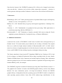
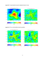
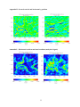
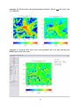
1
FOURPOT
Fourier transform based processing of 2D potential field data
Version 1.1
User's guide
Markku Pirttijärvi
July 2009
University of Oulu
Department of Physics
Geophysics
Table of contents
Table of contents ................................................................................................................... 2 1. Introduction ....................................................................................................................... 3 2. Installing the program........................................................................................................ 4 3. Menu items ........................................................................................................................ 5 3.1. File menu .................................................................................................................... 5 3.2. Edit menu.................................................................................................................... 5 3.3. Process menu .............................................................................................................. 7 4. Using the program ........................................................................................................... 11 4.1. Reading in the data ................................................................................................... 11 4.3. Padding and tapering ................................................................................................ 12 4.4. Fourier transform ...................................................................................................... 14 4.5. Inverse Fourier transform and the difference ........................................................... 15 4.6. Frequency filtering ................................................................................................... 15 4.6.1. Low pass and high pass filtering ...................................................................... 16 4.6.2. Directional filtering .......................................................................................... 17 4.6.3. Interactive and manual filtering ....................................................................... 17 4.7. Radial amplitude spectrum ....................................................................................... 19 4.8. Color mapping (range, center and levels) ................................................................. 20 5. File formats ...................................................................................................................... 22 5.1. Column formatted data files ..................................................................................... 22 5.2. Regularly gridded matrix files .................................................................................. 22 6. Graph options .................................................................................................................. 24 7. References ....................................................................................................................... 26 8. Additional information .................................................................................................... 26 9. Terms of use and disclaimer ............................................................................................ 27 10. Contact information ....................................................................................................... 27 Appendices A–N
Keywords: Potential fields, Fourier transform, FFT, 2D frequency filtering, data processing.
2
1. Introduction
The FOURPOT program is designed for frequency domain processing and analysis of twodimensional (2D) potential field arising, in particular, from geophysical gravity and magnetic
field measurements. The data can be irregularly or regularly sampled. The frequency domain
operations include high pass, low pass and directional filtering, upward and downward
continuation, pole reduction of magnetic data, 1.st and 2.nd degree vertical and horizontal (x
and y directed) gradients, total horizontal gradient, total gradient (analytical signal) and tilt
gradient. Pseudo-gravimetric and pseudo-magnetic fields can be computed also.
Considering a continuous function f(x) with continuous first derivatives the Fourier transform
F(kx) and its inverse transform can be written as (e.g., Blakely, 1995):
∞
F (k x ) =
∫e
− ik x x
and
f ( x ) dx
−∞
1
f ( x) =
2π
∞
∫e
ik x x
F (k x )dk x
−∞
Considering discrete and 2D data the governing equations are:
N
M
Fnm = ∑∑ e
− 2π i (
k =1 l =1
nk ml
+ )
N M
f kl
and
1
f kl =
NM
N −1 M −1 + 2π i ( nk + ml )
N M
∑ ∑e
n =0 m =0
Fnm ,
where N and M are the number of data values in x and y directions. The transform is complex
which means that it has both amplitude and phase spectra.
FOURPOT computes the discrete 2D Fourier transform using the fast Fourier transform
(FFT) algorithm. The Fourier transform represents a sum of sine and cosine terms with
different spatial frequencies (kx and ky) that are defined by data sampling (dx and dy) in x and y
directions. The highest spatial frequency is the so-called Nyquist frequency (e.g.,
max(kx) = 0.5/dx). The lowest frequency is based on the data coverage (e.g., min(kx) =
0.5/(max(x)-min(x)). Considering that the inverse of the spatial frequency represents wave
length (λx = 1/kx), zero frequency means infinite wave length, i.e., constant level of data.
Because of the properties of the Fourier transform (symmetry, linearity, shift and derivate
properties) several computational operations can be performed in Fourier transformed
frequency (kx, ky) domain more efficiently than in the spatial (x, y) domain. For more detailed
information about Fourier transform methods in potential field analysis, please, see Blakely
(1995), for example.
3
2. Installing the program
This version of FOURPOT is a 32-bit application that can be run on Windows XP/Vista
system with a graphics display of at least 1024×768 pixel resolution. Memory requirements
and processor speed and are not critical, unless very large data sets are used. The program has
simple graphical user interface (GUI) that is used to handle file input and output, to perform
the computational operations, and to visualize the data and the results. The user interface and
the data visualization are based on DISLIN graphics library.
The program requires these two files:
FOURPOT.EXE
the executable file an
DISDLL.DLL
dynamic link library for the DISLIN graphics.
The distribution file (FOURPOT*.ZIP) also contains a description file (_README.TXT),
this user's manual (FOURPOT_MANU.PDF), and some example data files (*.DAT). To
install the program uncompress (e.g., Winzip or 7Zip) the distribution file and move the
resulting FOURPOT folder to preferred place (e.g., C:\TOOLS). To be able to start the
program from a shortcut that locates in a different directory or from the desktop you should
move or copy the DISDLL.DLL file into the WINDOWS\SYSTEM (or SYSTEM32) folder
or somewhere along the system path.
4
3. Menu items
3.1. File menu
The File menu contains following options:
Read data
read in (irregularly spaced) data in default file format.
Read matrix
read in (regularly spaced) data in matrix format.
Save data…mat
save the data of current view in a matrix format.
Save data…dat
save the data of current view in general xyz column format.
Read disp.
read in new graph parameters from a *.DIS file.
Save Graph as PS
save the current graph in Adobe's Postscript format.
Save Graph as EPS
save the current graph in Adobe's Encapsulated PS format.
Save Graph as PDF
save the current graph in Adobe's PDF format.
Save Graph as WMF
save the current graph in Windows metafile format.
Save Graph as GIF
save the current graph in GIF file format.
These menu items bring up a standard (Windows) file selection dialog that is used to provide
the file name for I/O operations. All data files are in text format (see chapter 5). The graphs
are saved A4 landscape mode (see Appendix A). The preferred output format is PDF or PS,
because their resolution is much better than that of GIF and WMF files. The PDF format is
particularly useful because Adobe's Acrobat Reader can be used to take bitmap snapshots at
desired resolution.
3.2. Edit menu
The Edit menu contains following items:
Inverse→ data
set current results (of the inverse FFT) as new initial data.
Subtract inverse
subtract the inverse results from the original data.
Add inverse
add the inverse results to the original data.
Color scale
change the color scale (rainbow, gray scale, etc.).
Padding mode
change the method used to pad and taper data
Data type
define potential field data (generic, gravity, magnetic).
5
Miscellaneous
define some additional settings.
Low pass filter
perform (GUI directed or manual) low pass filtering.
High pass filter
perform (GUI directed or manual) high pass filtering.
Direction filter
perform (GUI directed or manual) direction filtering.
The use of Inverse→ data menu item can be used to put the current inverse results as new
input data for successive frequency domain operations. For example, tilt gradient can be
computed freom the upward continued data. Likewise, the Subtract inverse menu item allows
computing the residual field directly as the difference between the original (interpolated) data
and the upward continued or low pass filtered data. On the contrary, the Add inverse menu
item is used to add the inverse results to the original data. Although this item is not very
useful, it can be used to enhance high frequency content of the data, for example.
The Padding mode menu item is used to demonstrate the way padding and tapering is made.
Padding is an operation where null values are added around the original data area (see
Appendix B). The purpose of padding is to extend the data (N and M) to even power of two
(e.g. 64, 128, 256, 512 etc.) as the FFT algorithm requires this. Tapering is an operation
where the "padded" values are made such that they prevent rapid amplitude changes at the
border of the data area. This means that the data and their derivative are made more or less
continuous in padding. Together padding and tapering effectively remove so-called Gibbs
phenomenon as well as ringing and other artifacts in the inverse transformed data. Padding
will be discussed more in the next chapter.
FOURPOT does not consider what kind of data that are passed to it. Strictly speaking pole
reduction and pseudo-gravity, for example, are applicable to magnetic data only. For teaching
and testing purposes the Data type menu item allows defining the actual data type. In practice,
this has effect only on the information text next to the graph and the scaling of the radial
amplitude spectrum (see chapter 4.7).
The Miscellaneous menu item contains following items:
Contour/Image
change between contour map and image (pixel) map modes.
Show/Hide points
show/hide the actual data points in original data view.
Meters↔ Kilometers
swap units between meters and kilometers.
6
Reverse sign
reverse the sign of the original data.
Autom. low pass filter
automatic low pass filtering when activated.
Note: The information text next to the graph will show the dimensions incorrectly unless the
Meters↔ Kilometers menu item is utilized. Although knowledge about the spatial dimensions
is usually not required, the pseudo-gravity and pseudo-magnetic field need to know the real
dimensions for the amplitude of the transformed field to be more or less "truthful". The
Reverse sign item can be useful when working on the potential of the original field, since
often potential fields are defined as the negative gradient of the scalar potential.
The quality of some frequency domain filtering operations is strongly affected by the
"smoothness" and continuity of the data. To circumvent computational artifacts in the inverse
transformed data it is often necessary to perform low pass filtering before any other
processing operations. The Automatic low pass filter menu item activates automatic filtering
every time the FFT is computed. The inner and outer radii of the filter can be changed
manually using the dialog that appears after using the menu item. Note that the radii are not
defined as distances but as a ratio (a value between 0 and 1) of the minimum Nyquist
frequency of the data. Automatic values are used if the radii are set to zero. If the values are
omitted totally (i.e., a blank line is given) the automatic mode is deactivated.
Low pass and high pass filtering are the two most typical frequency domain processing
operations. Considering 2D data, low pass filtering removes (nullifies) values outside certain
radius from the origin of the frequency (amplitude) spectrum (see Appendices C, E and F).
On the contrary, high pass filtering removes low frequency data around the origin of the
spectrum. Together low and high pass filtering can be used as a band pass or notch filtering.
The direction filtering, which is applicable to 2D frequency data only, can be used to remove
or to enhance linear features in the original data (see Appendices G and H). The frequency
filtering can be accomplished either graphically with the mouse or manually using the given
numeric values. Frequency filtering will be discussed more in the next chapter.
3.3. Process menu
The Process menu contains the items for data processing operations:
7
Upward continuation
performs upward continuation.
Downward continuat.
performs upward continuation.
Pole reduction
performs reduction to magnetic pole.
dF/dz gradient
computes vertical gradient of the data.
dF/dx gradient
computes horizontal x gradient of the data.
dF/dy gradient
computes horizontal y gradient of the data.
d2F/dz2 gradient
computes second vertical gradient of the data.
d2F/dz2 gradient
computes second horizontal x gradient of the data.
d2F/dz2 gradient
computes second horizontal y gradient of the data.
d2F/dxdy gradient
computes xy gradient of the data.
2
d F/dxdz gradient
computes xz gradient of the data.
d2F/dydz gradient
computes yz gradient of the data.
Hori. gradient
computes horizontal gradient.
Total gradient
computes total gradient (analytic signal).
Tilt gradient
computes tilt gradient.
Pseudo gravity
computes pseudo-gravity field from magnetic data.
Pseudo magnetic
computes pseudo-magnetic field from gravity data.
Gravity potential
computes gravity potential from gravity field (Bouguer data).
Magnetic potential
computes magnetic potential from total field (TMI) data.
Undo process
reverts back to unprocessed (but frequency filtered) data
Upward continuation makes the data appear to have been measured higher above the surface
of the earth (or the plane of measurements). It is used to estimate the (low frequency) regional
trend of the data. Likewise, downward continuation makes the data appear to have been
measured below the plane of measurements, i.e., inside the earth. It is used to enhance the
high frequency content of the data and to estimate the depth to the top of the targets. Unlike
upward continuation, downward continuation is not a stable procedure. If the plane of
continuation is located below the actual potential field sources the results become erratic.
Examples of upward and downward continuation are shown in Appendix I.
Important: When performing upward or downward computation the height difference or
elevation is read from the Height text field in the control pane on the left side of the graph
area (see Appendix A). The height value is always positive, that is to say, the difference is
8
computed downwards or upwards depending on the selected task. The dimension of height is
the same as for the data itself (e.g., kilometers or meters depending on sampling).
Unlike gravity field the static magnetic field of a symmetric body (e.g vertical prism) exhibits
non-symmetric anomaly shape because the inclined direction of the inducing magnetic field.
The behavior of Earth's magnetic field can be estimated using the IGRF model (international
geomagnetic reference field). The Pole reduction item is used to transform magnetic field
data as if it were measured on a magnetic pole. This helps estimating the true dip and strike
directions of the targets.
Important: When performing pole reduction the inclination and the declination of the
magnetic field are read from the Incl. and Decl. text fields. The values are provided as angles
in degrees. Inclination (I = ±90°) is taken from horizontal plane and it is positive downwards
(northern hemisphere) and negative upwards (southern hemisphere). Declination (D = ±90°)
is positive in clock-wise orientation from the true north direction. The pole reduction is
unstable operation if the inclination is very small (near the equator).
The vertical and horizontal x and y gradients are used for the visual enhancement of some
features in the data. Both first and second degree gradients of the data f= f(x,y) can be
computed. Here x direction represents the horizontal axis and y direction the vertical axis of
the mapped data. The vertical gradients are particularly useful in enhancing the lateral
dimensions of anomalous sources (df/dz for magnetic data and d2f/dz2 for gravity data). The
less usual gradients d2f/dxdy, d2f/dxdz, d2f/dydz can be used to compute the off-diagonal
components of the gravity tensor provided that the gravity potential is first computed.
Examples of gradient operations are shown in Appendix J and K.
The horizontal gradient, h(x,y)= [d2f/dx2+d2f/dy2]1/2, total gradient a(x,y)= [d2f/dx2+d2f/dy2
d2f/dz2]1/2 (also known as analytical signal), tilt gradient t(x,y)= arctan[df/dz / h(x,y)] and the
horizontal gradient of tilt gradient s(x,y)= [d2t/dx2+d2t/dy2]1/2 are useful operations that can
used in visual interpretation of magnetic and gravity maps. They are used especially to
produce the location of lateral contacts of different geological units. Examples of these
gradient operations are shown in Appendix L and M.
9
Note: The horizontal gradient of tilt gradient s(x,y) can be computed manually as follows.
First the user needs to compute the tilt gradient t(x,y) and use Inverse→data menu item to
replace the original data. Then one computes the 2.nd horizontal x and y gradients d2t/dx2 and
d2t/dx2 and saves their results into two separate files. Finally, using a spreadsheet program one
computes the amplitude of the horizontal tilt gradient s(x,y)= [d2t/dx2+d2t/dy2]1/2.
The gravity and magnetic potentials (and hence the fields) of an anomalous target with the
same dimensions but different petrophysical properties (density and magnetic susceptibility)
are interrelated via Poisson's relation. The so-called pseudo-gravity field can be computed
from the measured magnetic data. Likewise, pseudo-magnetic field can be computed from
measured gravity data. For these operations some assumed values of density, susceptibility
and the intensity of the inducing magnetic field must be provided in the dialog that appears
after using the Pseudo gravity or Pseudo magnetic menu items. Also, as discussed in previous
chapter, the actual units of the spatial dimensions must be defined in order to compute the
amplitude of gravity effects. An example of pseudo-magnetic field is shown in Appendix M.
Note that the validity of the pseudo-magnetic and pseudo-gravity field computations has not
been verified in this version of FOURPOT. The potential of the gravity and magnetic field
data can be computed also. In the latter case the current values of field inclination and
declination are used to account for the direction of the inducing magnetic field.
The "Exit" menu has two items. The first one can be used restart the whole program in a mode
that is more suitable to widescreen or normal 4:3 displays. The second menu item is used to
confirm the exit operation. Before exit the user should save processed data, because they are
not saved automatically. Errors that are encountered before the GUI starts up can be found
from the FOURPOT.ERR file. When operating in GUI mode, run-time errors arising from
improper parameter values, for example, are shown on the display screen.
10
4. Using the program
When the program is started it reads graph parameters and some additional settings from the
FOURPOT.DIS file (see chapter 6 for more information). If this file does not exist, default
parameters will be assigned and the file is created automatically. The program then builds up
the GUI shown in Appendix A. None of the program controls (widgets), however, are active
before data has been read in.
The data processing and analysis is performed in few successive steps that are discussed next.
The preliminary step is always to check that the input data file is in correct format so that it
can be read in (see chapter 5 on file formats). After reading in the data one should apply Plot
matrix, Padding and Plot FFT buttons to perform interpolation and padding and to compute
the 2D frequency spectrum. Only after the FFT has been computed one can perform
frequency filtering (Edit menu) and frequency domain data processing (Process menu).
4.1. Reading in the data
The first thing to do after starting up the program is to read in the data using the Read data
(*.DAT) or Read matrix (*.MAT) menu items. Note that Geosoft XYZ formatted files can be
read as normal DAT files provided that the file header is added by hand. See chapter 5 for
more information about file formats.
After successful data input the program automatically interpolates the data on a regular grid
and plots a contour map as seen in Appendix A. The initial grid sampling is based on the
number of data values and the spacing between the first two data points in the file. The grid
dimensions, i.e, the number of grid nodes in x and y directions (N and M) will appear in Dim x
and Dim y text fields in the control pane. At any time the original data can be plotted again
with the automatic grid spacing using the Plot data button.
4.2. Interpolation
All input data are assumed to be irregularly sampled. Even if the original data were already
evenly discretized it will be re-interpolated before it's passed to FFT. Therefore, after reading
in the data the user must always apply the Plot matrix button, which is used to perform the
11
required interpolation using the grid dimensions (N and M) provided on the Dim x and Dim y
text fields. Note that the grid spacing (dx and dy) does not need to be equal in x and y
directions.
The Plot data function is used merely to visualize the original data and it does not affect the
current grid dimensions. If the grid dimension changes from the default or initial values
(because of interpolation or padding), one can revert back to original (automatically
computed) sampling using the Def size button. The Aspect ratio button, on the other hand, is
used to reset either the Dim x or Dim y dimension so that the original shape of the data area is
preserved. This means that when a new value of Dim x or Dim y is given, the other value is set
so that the original aspect ratio remains when Aspect ratio button is applied.
Important! The horizontal and vertical dimensions (N and M) of the data matrix passed to the
FFT algorithm must be powers of two (e.g., 64, 128, 256, 512, etc.). The interpolation
discussed above is performed using the GETMAT subroutine included in the DISLIN
graphics library (see DISLIN user manual). This subroutine works best if the data are already
regularly sampled and the dimensions coincide with the original grid. Therefore, it is
recommended that highly irregular data are interpolated on a regular grid using a more
advanced third party software (e.g., Golden Software Surfer) and more suitable algorithm
(e.g, minimum curvature). Naturally, if evenly discretized data are passed to FOURPOT one
should take care that the interpolation (Plot matrix) is made using the same grid sampling as
that of the original data so that as minimal distortion is made by GETMAT as possible.
4.3. Padding and tapering
Padding and tapering are essential parts of successful Fourier transform processing. The
Padding button will automatically add extra columns and rows around the interpolated data
matrix so that the grid dimensions (N and M) will increase to the next even power of two (see
Figure 4.1 and Appendix B). The padding can be performed with or without tapering.
Tapering means that the padded data are such that the level and the derivative of the data are
preserved.
Sometimes the original grid dimension may already be so close to some power of two that the
tapering will not have enough time to suppress data discontinuity. To further increase the
12
padded dimension from 64 to 128, for example, one simply needs to change the current value
of Dim X or Dim Y to some number between 65 and 128. This will then be adjusted to 128
when Padding button is pressed. Note that the dimension of the grid can be decreased only
using re-interpolation by Plot matrix button.
a) normal padding
b) shifted padding
b) padding + tapering
M'
padded values
tapered values
original data
area
original data
area
padded values
tapered values
padded values
M
original data
area
0,0
N
N'
0,0
N'
0,0
N'
Figure 4.1. Schematic view of a) padding without shift, b) padding with shift and c) shifted
padding with tapering. The new dimensions N' and M' are powers of two.
Padding and tapering depend on the selection made with the Padding mode item in Edit
menu. The padding modes are: a) Zeros which actually use the median of the outmost data
points instead of zeros for padding, b) Linear extrapolation will extend with the outmost data
point, c) Mean value based will use the nearest points inside some increasing search radius
and d) Gradient based, which uses the mean value and the derivative of the field to extend the
data to the padding zone. The Shift yes/no option is used to define if padding is added only to
the top and to the right of original data area or if padding is made all around the data area
(which looks like the data were shifted).
Important! Best results from Fourier transform processing are obtained using gradient based
padding with shift. The other padding options are kept primarily for teaching purposes so that
the users can see the effect and importance of padding and tapering.
13
4.4. Fourier transform
After sampling, interpolation and padding one can use the Plot FFT button to compute the
FFT and to see the 2D frequency spectrum (see Appendix C).
At this point one should remember that the frequency spectrum F is complex, i.e., it has both
real and imaginary parts, F = Re(F) + i⋅Im(F). Thus, the 2D Fourier graph actually represents
the 10-base logarithm (log10) of the amplitude spectrum A = (Re(F)2 + Im(F)2)1/2. The origin
(kx=0, ky=0) of the graph is located at the middle of the graph and the horizontal and vertical
axis range between the Nyquist frequencies, the value of which are shown in the information
text next to the graph. Lowest frequencies or largest wave length (long variations of data) are
located in the middle of the graph and highest frequencies or shortest wave lengths (short
variations of data) are located far from the origin. Continuous linear features in the data
appear as linear features in the FFT spectrum as well (the angle of slope is inversed, though).
Only after the FFT has been computed one can perform the frequency filtering and other
frequency domain processing. The inverse FFT and the difference between the original
(gridded) data can be plotted using Inverse FFT and Plot.
Note that each Fourier operation is made on the interpolated and padded data matrix (Plot
matrix/Padding). Multiple Fourier operations (e.g. pole reduction and total gradient) can be
performed in a row by using the Inverse→Data menu item after the first operation and
performing new FFT and the second Fourier operation. Alternatively, one can save the current
inverse results and restart the program using the saved results as new input data.
14
4.5. Inverse Fourier transform and the difference
After the Fourier transform and the 2D frequency spectrum has been computed one can
perform frequency filtering tasks in the Edit menu and/or any of the frequency domain
processing tasks in the Process menu. The Plot inverse button can be used to display the
current inverse results, that is to say the either the inverse FFT of the current frequency
(filtered and/or processed) spectrum. When tasks are selected from the Process menu the
inverse results will be shown automatically.
Successive utilization of the Plot inverse and Plot data buttons can be used to visualize the
changes that are made to the data due to the frequency domain operations. As an alternative,
the Plot diff button can be used to visualize the difference between the original (interpolated)
data and the data obtained from the inverse FFT after the most recent Fourier operation. If no
operations have been made the inverse will be and should be (almost) equal to the original
data. Note that pressing the Def. size or Padding buttons will invalidate the current frequency
spectrum and inverse results and the user needs to perform the frequency filtering operations
again. Note also that after Padding the Plot matrix function becomes inactive, because the N
and M values are affected by the padding to the next power of two. To be able to re-grid the
original data one needs to aplly the Def. size button.
4.6. Frequency filtering
Important: Unlike the other processing operations, frequency filtering affects the current
amplitude spectrum on which other processing functions are performed and from which the
inverse transform is computed. This means that frequency filtered data are always passed to
further processing operations without the use of Inverse→ data menu item. As a matter of
fact, low pass filtering is often an essential preliminary step for successful operation of the
gradient filters.
Like the rapid changes in the data can cause problems when its FFT is processed, rapid
changes in FFT spectrum can cause oscillations in the inverse transformed data. This is
known as the Gibbs phenomenon. Therefore, instead of using an abrupt box-car shaped filter
function a smooth bell shaped (sine and cosine) functions are applied over certain cut-off
range. In low pass and high pass filtering this means in practice that instead of a single radius
of a single filter ring one needs to provide the radii for the inner and outer ring of the cut-off
15
range separately. Between the two rings the filtering is made using a quarter sine or cosine
functions. Likewise, in directional filtering one needs to provide three values that define the
upper and lower sector range and the width (as an angular difference) of the cut-off range.
The filter rings and sectors and the cut-off ranges are illustrated in Figure 4.2.
b) 2D direction filter
a) 2D low pass filter
all values
nulled
cut-off
range
cut-off
ranges
all values
preserved
inner ring
upper and
lower sector
range
outer ring
c) low pass filter
d) high pass filter
e) band pass filter
1
1
1
0
0
0
k=0
k=0
k=0
Figure 4.2. Schematic view of a) cut-off rings and b) sectors of 2D filters and the smooth
(bell shape) filter function of c) low-pass, d) high pass and e) band pass filters.
4.6.1. Low pass and high pass filtering
In low pass filtering all data outside the outer ring (high frequencies) are nullified and all data
inside the inner ring are preserved (see Figure 4.2a and c). On the contrary, in high pass
filtering all data inside the inner ring (low frequencies) are nullified and all data outside the
outer ring are preserved (see Figure 4.2d). The radius of the rings are defined as wave length
(λ), which is the inverse of radial frequency kr= [kx2+ky2]1/2, where kx and ky are the axes of the
2D frequency graph. The unit of the wave length is either meter or kilometer depending on
the selection made using the Meters↔ Kilometers item in the Edit-Miscellaneous menu.
16
Note: If the sampling intervals are different in the x and y directions the spatial frequencies (kx
and ky) will be different also. Because, a single value of wave length is used as filter
dimension both in x and y directions, the filter rings will appear as an ellipses instead of
circles in the 2D frequency graph.
4.6.2. Directional filtering
Directional filtering is equal to the so-called fk-filtering commonly used in seismic and GPR
data processing. Directional filtering removes (or enhances) linear features with certain angle
in the data. In directional filtering the data are removed inside two sectors that are symmetric
around the origin (see Figure 4.2b). The filter removes the frequency data inside a sector
defined by two angles that correspond to the upper and lower limit of the sector. The angles
are defined in degrees in counter-clockwise direction taken from the positive kx axis. In
addition, the cut-off range is defined by providing a third parameter as an angular difference
either from the upper or the lower sector (the width of the cut-off range will be the same on
both sides). Because of the symmetry of the frequency spectrum the directional filter will be
mirrored around the origin automatically. Thus, one needs to define only single sector either
above the kx axis or left to the ky axis.
4.6.3. Interactive and manual filtering
Filtering can be done either a) interactively using the mouse or b) manually by providing the
numerical values of the filter cut-off ranges. The selection is made when the corresponding
menu item is chosen in the Edit menu.
When interactive mode is chosen most of the other program widgets become inactive and the
mouse cursor changes from normal arrow into a cross-hair above the graph area (note: only
above the graph area). The 2D frequency spectrum is shown together with auxiliary polar
coordinate system grid. The user is given instructions to provide first the inner and then the
outer ring by pressing the left mouse button above the graph. To validate the last value and to
end the editing mode one must press the right mouse button. The distance from the origin
determines the radius of the filter rings. Likewise in directional filtering the user is instructed
to provide the upper and lower angle of the filter sector and the width of the cot-off range.
17
The width can be defined as a angular difference from the lower or upper sector and the filter
cut-off range will be adjusted symmetrically at both sides automatically.
Note that the ring and sector values can be provided in reverse order in which case they will
be automatically arranged so that the inner ring is smaller than outer ring or the upper angle is
larger than lower angle. Values can be omitted by pressing the right mouse button instead of
the left one. In low pass and high pass filtering omitting the first value cancels the whole
interactive editing mode. Omitting the second value will make the two rings the same which
means that the sine/cosine bell function is replaced by a box-car filter. In directional filtering
the upper and lower angle must always be provided but the cut-off range can be omitted if the
right mouse button is pressed when its value is asked for.
Important: After interactive editing the given filter rings and sectors will be shown by dotted
lines on the frequency spectrum. The wave lengths and the angles will appear in the Ring 1,
Ring 2, Sect 1, Sect 2 and Taper text fields in the left control pane. Their values, however, are
not stored if multiple filtering are made in this version of FOURPOT. Also note that together
low and high pass filtering can be used to accomplish band pass and notch filtering. The Ring,
Sect and Width text fields, however, will show the parameters of the last filtering only.
Therefore, the user should remember to memorize or save the parameters of the frequency
filters because they may be needed to reproduce the processing results afterwards.
After the user gets accustomed with interactive filtering one should learn manual filtering
which is more accurate than interactive filtering. Manual filtering is made by providing the
wave lengths (in units of dimension) of the filter rings (low pass and high pass filtering) or the
angles of (in degrees) the filter sectors and width of the cut-off range (directional filtering) in
directly the corresponding Ring 1, Ring 2, Sect 1, Sect 2 and Width text fields in the left
control pane. Then by selecting the desired menu item from the Edit menu one can perform
low pass, high pass or direction filtering. Some default parameters are used if the text fields
are equal to zero.
18
4.7. Radial amplitude spectrum
The Radial spectrum button, which is active only when the 2D frequency spectrum is active,
will compute the amplitude spectrum as a function of the radial frequency. The radial
amplitude is the mean of the 2D Fourier amplitude spectrum A= |F|= [Re(F)2+Im(F)2]1/2 along
rings with radius kr= [kx2+ky2]1/2. The amplitude spectrum has traditionally been used to
estimate the depth to the bottom of potential field sources. This is established by fitting linear
lines to the decaying amplitude curve on a semi-logarithmic scale. An example is shown in
Figure 4.3.
Figure 4.3. Radial amplitude spectrum with two manually fitted lines. The slopes give
estimates for the depth to the bottom of the potential field sources.
In frequency domain the Fourier transform of a potential field can be formulated as F≈Ce-hk
giving log(F/C)= -h⋅kr. Thus, the depth to the top of an anomaly source (h) is equal to the
tangent or the slope of the linear parts of the amplitude spectrum. For general data type the
coefficient C= 1 and the vertical axis is the logarithm of the amplitude spectrum, log|F|. For
gravity data the coefficient C= -1/(kxkykr), and in case of magnetic data C=-1/(kxky) (selected
by the Data type item in Edit menu). Because of the data type the slopes and, therefore also
19
the depth estimates are quite different. Depending on the data the normalization might not be
useful at all, so one should prefer to general data type. Please, refer to Bhattacharyya (1967)
and Ruotoistenmäki (1987) for more information about the use of radial amplitude spectrum
for depth determination. Note that the depth interpretation option has not been fully tested in
this version of FOURPOT.
Interactive line fitting is accomplished by pressing the Define line button when radial
amplitude spectrum is displayed. The mouse pointer changes into a cross-hair cursor over the
graph area. The user should select the start and end points of the line over the scattered data
plot of the radial amplitude spectrum by pressing the left mouse button. The editing mode is
ended by pressing the right mouse button. The graph will be redrawn with the newly edited
line on it and the slope of the line will be displayed on the information text on the right side of
the graph. Multiple lines can be added to the same graph pressing the Define line button
again. The most recent line can be deleted from the graph pressing the Delete line button.
Note: Low pass and high pass filtering affect the computation of the radial spectrum. Because
of the cut-off range of the filters the radial spectrum may look quite different from the one
shown in Fig. 4.3, for example. Also note that the vertical axis of the radial spectrum (and 2D
spectrum as well) is logarithmic and that the nulled values are plotted as zeros on the logscale. Naturally this means that nulled values are plotted incorrectly (they are really zeros).
4.8. Color mapping (range, center and levels)
The Range and Center scale widgets can be used to change the color mapping of the data
maps and 2D frequency spectrum. The Levels widget is used to define the number of contour
levels (the default is 21 levels).
By default the color scale (eg. rainbow or reverse rainbow) is evenly distributed between the
minimum and the maximum data values of the current map. The Range widget allows
changing the range of the color scale by between 5 % and 125 % of the original minimum
and maximum values. Decreasing the value is useful if the maximum data value of the map is
larger than the mean data level due to outlier, for example. Increasing its value is useful if the
maps get saturated at their minimum or maximum limit values.
20
The Center scale widget changes the middle point of the color scale between -85 % and
+85 % of the current data range. Increasing the center value will emphasize small data values
and increases the amount of colors at the beginning part of the color scale. Decreasing the
center value will emphasize large data values and increases the amount of colors at the end of
the color scale.
Important: After changing any of the abovementioned scales one needs to press the Update
plot button to make the changes visible. Because the scale widgets give different results for
different graphs one can reset the color mapping parameters to their defaults using the Reset
scale button.
Note that FOURPOT was not designed to be used as a plotting program. To prepare the final
results the user is advised to use plotting programs like Golden Software's Surfer.
21
5. File formats
Potential field data can be read into FOURPOT in two file formats: a) generic column
formatted data file (*.DAT) and b) regulary gridded data matrix (*.MAT).
5.1. Column formatted data files
The format of a *.DAT file is illustrated below:
4096 1
0.00
10.00
20.00
...
2
4
0.00 -0.8665106E+01
0.00 -0.8558651E+01
0.00 -0.8365253E+01
0.33489
0.44134
0.63474
The data file can contain multiple columns and the header line at the first line is used to define
the number of lines (NOP) and the indices of the columns that contain the x and y coordinates
(ICO1, ICO2) and data (ICO3). FOURPOT ignores empty lines and lines starting with ", /, l,
L or # characters. Thus, provided that NOP is large enough ICO* refer to correct column
indices, FOURPOT can also read Geosoft XYZ files (*.XYZ) illustrated below:
5000 1
2
4
/ Test data
LINE 1
0.00
0.00 -0.8665106E+01
10.00
0.00 -0.8558651E+01
20.00
0.00 -0.8365253E+01
...
LINE 2
0.00
10.00 -0.8165106E+01
10.00
10.00 -0.8258651E+01
20.00
10.00 -0.8465253E+01
...
0.33489
0.44134
0.63474
0.23489
0.34134
0.53474
Note: The header line can be omitted in which case the program shows the first line of the
data file and asks the parameter (NOP, ICO1, ICO2, ICO3) values from the user.
5.2. Regularly gridded matrix files
The matrix format (*.MAT) expects that the data are stored in a regular grid without x and y
coordinates. The matrix format is provided for easier functionality with programs such as
Matlab and Maple. The format of a matrix file (*.DAT) is illustrated in the example below:
22
64
64
-0.43160E+09
-0.43320E+09
-0.43270E+09
...
The header line defines the number of data points in x and y directions (NP and MP). The
following (NOP = NP × MP) lines contain the actual data values. Note that because the matrix
format does not contain coordinates the sampling frequencies and corresponding wave lengths
shown by FOURPOT are not correct if they are not provided correctly in the dialog that
appears after the matrix data are read in. The dialog window is used to define the x and y
coordinates of the origin and the x and y step between the matrix elements. Note that if the x
and/or y steps are negative, the axis gets reversed. Moreover, the data are mirrored in x or y
direction if the last two parameters from zero to one in the auxiliary dialog.
Since the matrix file does not contain coordinates it is important to know the order in which
the data are stored. The origin is always located in the bottom left corner. By default the data
is stored in column-wise fashion from bottom to top and from left to right. Using a generic
programming language notation we would have:
do i= 1,np
do j= 1,mp
read or write f(i,j)
end do
end do
When matrix data are read in, the order can be changed so that for each column the rows will
be read by giving a negative value for the number of points in x direction (NP= -NP).
Furthermore, if MP < 0 the matrix file is considered to have multiple data columns which will
be read row by row (the file really looks like matrix). If NP > 0 and MP < 0 the rows are
considered to be the y columns of the mapped data as in the default case. If NP < 0 and
MP < 0 the rows are considered to be data rows (but the origin is still in lower left corner).
Using a generic programming language notation we would have in this case:
do j= 1,mp
read (f(i,j), i=1,np)
end do
23
6. Graph options
Several graph parameters and text strings can be changed by editing the FOURPOT.DIS file.
This allows one to localize the graphs into another language, for example. Note that if the
format of the FOURPOT.DIS file is important. If the format of the file becomes invalid, one
should delete the file and a new one with default parameter values will be generated
automatically next time the program is started. The file format is illustrated below:
# Fourpot ver.
36
32
0
0
350
600
75.0
1.10 parameter file
24
2
0.90
10.0
0
0
1
0
1
0.80 0.91 0.00
52000.0 1.00000
0
0
0.00 0.00
0.01000
0.0
2-D Fourier transform analysis
Original data
Interpolated data
Transformed data
Inverse data
Difference
Radial ave. spectre
X
Y
Field
Kx
Ky
log10(F)
Kr
log(F)
Low pass filtered
High pass filtered
Direction filtered
Upward continued
Downward continued
Pole reduced
dF/dz gradient
dF/dx gradient
dF/dy gradient
d^2$F/dz^2$ gradient
d^2$F/dx^2$ gradient
d^2$F/dy^2$ gradient
d^2$F/dxdy gradient
d^2$F/dydz gradient
d^2$F/dydz gradient
Horizontal gradient
Total gradient
Tilt gradient
Pseudo gravity
Pseudo magnetic
Gravity potential
Magnetic potential
Unprocessed data
24
0
0.0
• The two first lines are used as a header to identify the file and version number.
• The 1.st actual data line defines three character height values. The first one is used for the
main title, the second one is for the axes labels and the third one is used for the plot legend.
• The 2.nd line defines some integer valued options. The first one sets the screen mode
between screen normal 3:4 aspect ratio and wide screen mode. The second one defines the
color scale. The third and the fourth parameter define padding and tapering modes. The
fifth parameter sets either contour or image map mode. The sixth parameter defines the use
of automatic low pass filtering mode. The extra parameters are reserved for future use.
• The 3.rd line defines the x- (horizontal) and y- (vertical) distance (integer values) of the
origin of the main graph (in pixels) from the bottom-left corner of the page, and the length
of the x- and y-axis relative to the size of the remaining (origin shifted) width and height of
the plot area. The total size of the plot area is always 2970×2100 pixels (landscape A4).
The fifth parameter defines the aspect ratio of the graph area when widescreen mode is
used. The remaining parameters are reserved for future use.
• The 4.th line defines the initial values of the magnetic and gravity field components used in
pole reduction and pseudo-field computations. These parameters include: the inclination
and declination (in degrees from horizontal plane and true north) and intensity (in nanoTeslas) of the magnetic field, the density contrast (in grams per cubic centimeter) and
susceptibility (dimensionless in SI units).
• The 5.th line should be left empty.
• The following 15 lines define various text items of the graphs. These include: the main title
of the graph, the 6 possible sub-titles of the graph, the axis labels and color scale label of
the data in spatial domain, the axis labels and color scale label of the data in frequency
domain, the axis labels of the graph of the radial spectra. The maximum length of each text
string is 70 characters.
• The 16.th line between the two text blocks should be left empty.
• The last 23 lines define various text items (max. 70 characters) that are shown in the
information text next to the graph. These include the (possible) filtering operations made to
the FFT data and the processing operation made to the inverse FFT data.
25
Note that the format of the FOURPOT parameter file is likely to be changed in the future.
Also note that the ^ character can be used to define superscripts (exponent), _ character is
used to generate subscripts, and the $ character is used to move the text back to the baseline.
7. References
Bhattacharyya, B.K., 1967. Some general properties of potential fields in space and frequency
domain; a review. Geoexploration, 5, 127-143.
Blakely, R.J., 1995. Potential theory in gravity and magnetic applications. Cambridge Univ.
Press.
Claerbout, J., 1976. Fundamentals of geophysical data processing. With applications to
petroleum prospecting: McGraw-Hill Book Co.
Ruotoistenmäki, T., 1987. Estimation of depth to potential field sources using the Fourier
amplitude spectrum. Bulletin 340, Geological Survey of Finland. (PhD thesis).
8. Additional information
I made the first version of FOURPOT in 2003 when I worked at the Geological Survey of
Finland for the 3-D crustal model project funded by the Academy of Finland. The original
idea was to utilize the depth analysis methods of Ruotoistenmäki (1987). In 2005, when I
started as a lecturer of applied geophysics in Oulu the objective became more educational and
I have used FOURPOT in the teaching of gravity and magnetic data processing.
The Fourier transform is based on the FFT algorithm FORK by Jon Claerbout (1976). Look
for his webpage via Stanford Exploration Project (http://sep.stanford.edu) for more details.
Thanks to Richard Stuart for the comments on smooth frequency filtering. More information
about the geophysical use of Fourier transform methods in potential field processing can be
found in Blakely (1995), for example.
The FOURPOT program is written in Fortran 90 style using Intel Visual Fortran version 11.1.
The graphical user interface is based on the DISLIN graphics library version 9.4 by Helmut
Michels. For more information, please, visit http://www.dislin.de. Because the DISLIN
graphics library is independent form the operating system, FOURPOT could be compiled on
other operating systems (Solaris, Linux, Mac OS X) without large modifications. At the
26
moment, however, the source code is not made available and I do not provide any support for
the software. However, if you find the results erroneous or if you have suggestions for
improvements, please, inform me.
9. Terms of use and disclaimer
The FOURPOT software is totally free for personal and scientific use. If you find it useful,
please, send me a postcard. If you decide to use results computed with FOURPOT in
publications,
please,
use
this
user
manual
and
the
web
page
at
http://www.cc.oulu.fi/~mpi/softat as a reference, because I have not (yet) published this work
in any journal.
The FOURPOT program is provided as is. The author (MP) and the University of Oulu
disclaim all warranties, expressed or implied, with regard to this software. In no event shall
the author or the University of Oulu be liable for any indirect or consequential damages or
any damages whatsoever resulting from loss of use, data or profits, arising out of or in
connection with the use or performance of this software.
10. Contact information
Markku Pirttijärvi
Department of Physics
P.O. Box 3000
FIN-90014 University of Oulu
Finland
Tel: +358-8-5531409
Fax: +358-8-5531484
E-mail: markku.pirttijarvi(at)oulu.fi
URL: http://www.gf.oulu.fi/~mpi
27
Appendix A. FOURPOT GUI after data input
Appendix B: Data map after padding (with shift) and tapering
28
Appendix C: 2D frequency (amplitude) spectrum
Appendix D: Difference between original data and inverse transformed data
29
Appendix E: Low pass filtered frequency spectrum
Appendix F: Low pass filtered data and its difference to original data
30
Appendix G: Direction filtered frequency spectrum
Appendix H: Direction filtered data and its difference to original data
31
Appendix I: Upward and downward continued data (h= 2 km)
Appendix J: First vertical and horizontal x gradient
32
Appendix K: Second vertical and horizontal y gradient
Appendix L: Horizontal gradient and total gradient (analytical signal)
33
Appendix M: Tilt derivative and pseudo-magnetic field (k= 0,01 SI, Δρ= 0,2 g/cm3, and
T0= 52000 nT)
Appendix N: Program GUI with 2.nd vertical gradient after low pass filtering and
modification of the color scale
34