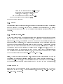
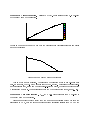
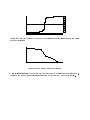
1
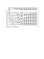
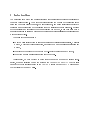
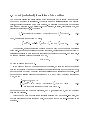
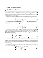
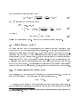
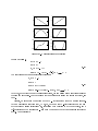
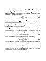
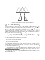
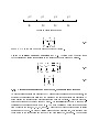
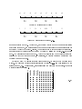
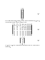
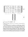
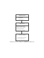
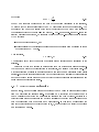
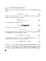
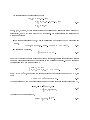
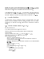
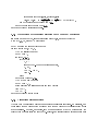
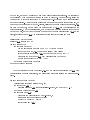
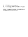
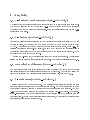
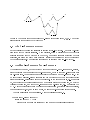
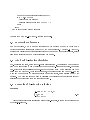
1D hp-ADAPTIVE FINITE
ELEMENT PACKAGE
FORTRAN 90 IMPLEMENTATION
(1Dhp90)
Leszek Demkowicz and Chang-Wan Kim
Texas Institute for Computational and Applied Mathematics
The University of Texas at Austin
Austin, TX 78712
Abstract
This manual provides a description of a 1D hp-adaptive nite element code for the
solution of a class of two-point boundary-value problems. The implementation is based
on hierarchial shape functions and allows for both h; and p; renements of the mesh,
based on a posteriori error estimation. The code includes an automatic hp-adaptive
strategy. Numerical results for several test problems illustrate the method.
Contents
1 Introduction
4
2 A General Two-Point Boundary Value Problem
5
3 Finite Element Method
9
2.1 Strong, or classical, form of the problem . . . . . . . . . . . . . . . . . . . .
2.2 Weak (variational) formulation of the problem . . . . . . . . . . . . . . . . .
3.1 Galerkin approximation . . . . . . . . . . . . . . . . . . . . . . . . . . . . .
3.2 Finite Element Method . . . . . . . . . . . . . . . . . . . . . . . . . . . . . .
3.2.1 1D master element of an arbitary order . . . . . . . . . . . . . . . . .
3.2.2 A 1D parametric element of arbitrary order . . . . . . . . . . . . . .
3.2.3 1D hp nite element space. . . . . . . . . . . . . . . . . . . . . . . . .
3.2.4 Element stiness matrix and load vector . . . . . . . . . . . . . . . .
3.2.5 Taking into account the boundary conditions. Modied element matrices
3.2.6 Global stiness matrix and load vector, the assembling procedure . .
3.3 Structure of a classical FE code . . . . . . . . . . . . . . . . . . . . . . . . .
5
6
9
10
10
12
14
15
16
17
20
4 Error estimation
23
5 User Manual
27
4.1 A priori error estimation . . . . . . . . . . . . . . . . . . . . . . . . . . . . . 23
4.2 A posteriori error estimation . . . . . . . . . . . . . . . . . . . . . . . . . . . 24
4.2.1 The element implicit residual method . . . . . . . . . . . . . . . . . . 25
5.1
5.2
5.3
5.4
Data structure in 1Dhp90 . . . . . . . . . . . . . . . . . . . . . . . . . .
Organization of the code . . . . . . . . . . . . . . . . . . . . . . . . . . .
Mesh generation and postprocessing routines . . . . . . . . . . . . . . . .
Processing algorithms . . . . . . . . . . . . . . . . . . . . . . . . . . . . .
5.4.1 Evaluation of element matrices (elem pack/elem.f) . . . . . . . . .
5.4.2 Modication of the element matrices due to boundary conditions .
5.4.3 Assembling global matrices . . . . . . . . . . . . . . . . . . . . . .
.
.
.
.
.
.
.
.
.
.
.
.
.
.
27
27
28
29
29
30
30
5.4.4 Solver . . . . . . . . . . . . . . . . . . . . . . . . . . . . . . . . . . . 32
5.4.5 Setting up data. Files . . . . . . . . . . . . . . . . . . . . . . . . . . 32
6 Adaptivity
6.1
6.2
6.3
6.4
6.5
6.6
6.7
6.8
6.9
34
p-renement/unrenement(meshmods pack/modord.f ) . . . . . . . . . . . . 34
h-renement (meshmods pack/break.f ) . . . . . . . . . . . . . . . . . . . . . 34
Natural order of elements (datastrs pack/nelcon.f )
h-unrenement(meshmods pack/cluster.f ) . . . . .
The h-renements strategy . . . . . . . . . . . . . .
Trading h-renements for p-renements . . . . . . .
Interactive renements . . . . . . . . . . . . . . . .
The nal hp-adaptive algorithm . . . . . . . . . . .
Examples of hp-adaptive solutions . . . . . . . . . .
A Interface with a frontal solver
.
.
.
.
.
.
.
.
.
.
.
.
.
.
.
.
.
.
.
.
.
.
.
.
.
.
.
.
.
.
.
.
.
.
.
.
.
.
.
.
.
.
.
.
.
.
.
.
.
.
.
.
.
.
.
.
.
.
.
.
.
.
.
.
.
.
.
.
.
.
.
.
.
.
.
.
.
.
.
.
.
.
.
.
.
.
.
.
.
.
.
.
.
.
.
.
.
.
34
34
35
35
36
36
36
42
1 Introduction
The nite element method is a general technique for constructing approximate solutions to
boundary value problems. The method involves dividing the domain of the solution into a
nite number of simple subdomains, the nite elements, and using variational concepts to
construct an approximation of the solution over the collection of nite elements. Because
of the generality and richness of the idea underlying the method, it has been used with a
remarkable success in solving a wide range of problems in virtual all areas of engineering and
mathematical physics.
The goals of this manual are :
to give a brief introduction to fundamental ideas of variational formulation, Galerkin
method, a posteriori error estimation, in context of a one dimensional nite element
method,
to introduce the reader to the concept of hp-adaptive Finite Element Methods,
to provide a minimal user information for the package.
Consequently, we have decided to write this document in a format of lecture notes.
Indeed, it is our intention to use the notes in the ASE384P/EM 394F/CAM394F(Finite
Element Methods) [4] class taught in the ASE/EM Department and the CAM programs at
the University of Texas at Austin.
2 A General Two-Point Boundary Value Problem
2.1 Strong, or classical, form of the problem
We begin by considering a two-point boundary value problem of nding a function u =
u(x); x 2 [0; l]. The strong form of the boundary-value problem consists of a second order,
ordinary dierential equation,
;(a(x)u(x)0 )0 + b(x)u0 (x) + c(x)u(x) = f (x) x 2 (0; l);
(2.1)
accompanied at each of the endpoints x = 0 or x = l with one of three possible boundary
conditions:
Dirichlet boundary condition,
u(0) = 0 or u(l) = l ;
(2.2)
Neumann boundary condition,
;a(0)u0(0) = 0 or a(l)u0(l) = l ;
(2.3)
Cauchy boundary condition
;a(0)u0(0) + 0u(0) = 0 or a(l)u0(l) + l u(l) = l:
(2.4)
The Neumann boundary condition is just a special case of Cauchy boundary condition with
constant = 0. For discussion of other possible boundary conditions including periodic
boundary conditions, see [4].
The data for the problem consist thus of :
coecients of the dierential operator a(x); b(x); c(x) (the material constants),
right-hand side f (x) (the load ),
boundary conditions data ; .
2.2 Weak (variational) formulation of the problem
The weak formulation is a reformulation of the strong form and it is from this weak form
that the FE approach is established. Whenever a smooth classical solution to a problem
exists, it is also the solution of the weak problem. To establish the weak form of the strong
form given by equation (2.1), multiply (2.1) by an arbitary, so called, test function v(x), and
integrate over interval (0; l). We obtain
Zl
0
[;(a(x)u0 (x))0 + b(x)u0 (x) + c(x)u(x)] v(x) dx =
Next, we integrate the rst term by parts,
Zl
0
Zl
au0v0 dx ; au0v jl0 + 0 bu0v dx +
Zl
0
cuv dx =
Zl
0
Zl
0
f (x)v(x) dx:
(2.5)
f (x)v dx :
(2.6)
At this point, further derivation depends upon the kind of the boundary conditions
being used. In the case of Dirichlet boundary condition, we eliminate the boundary term by
restricting ourselves to only those test functions that vanish at that point. For example, if
we assume Dirichlet boundary condition at x = 0,
u(0) = (0);
(2.7)
we have to assume that v(0) = 0.
In the case of Cauchy or Neumann boundary condition, we build the boundary condition
into the formulation by using it to calculate the derivative in terms of the boundary data,
and (in the case of Cauchy boundary condition) still unknown solution at that point. Thus
in the case of Dirichlet boundary condition at x = 0 and Cauchy boundary condition at
x = l, we get
8
>
Find u(x); u(0) = 0
>
>
Z
<Zl
0 v 0 + bu0 v + cuv ) dx + u(l)v (l) = l f (x)v dx + v (l)
(
au
l
l
>
>
0
0
>
:
for every test function v(x) such that v(0) = 0:
(2.8)
In the case of Neumann boundary condition, at x = l, constant l = 0, and the boundary
term simply vanishes.
Notice that we have kept all terms involving solution u(x) on the left-hand side, and
the terms involving the test function v only, have been moved to the right-hand side of the
equation.
The weak (variational) formulation can be shown to be equivalent 1 to the classical form
of the boundary-value problem. We integrate back by parts and use the Fourier lemma
argument to recover the dierential equation and Cauchy (Neumann) boundary condition at
x = l. Notice that there is no need to recover Dirichlet boundary condition, as it has been
simply rewritten into the weak formulation.
A precise mathematical setting is obtained by introducing the Sobolev space of the rst
order H 1(0; l), consisting of functions that are, together with their derivatives, square integrable,
Zl
Zl
1
2
H (0; l) = fv(x) : 0 v dx; 0 (v0)2 dx < 1g:
(2.9)
Next, we identify the subspace of kinematically admissible functions V, satisfying the homogeneous Dirichlet boundary condition,
V = fv 2 H 1(0; l) : v(0) = 0g:
(2.10)
The set of functions satisfying the nonhomogeneous Dirichlet boundary condition has a more
complicated algebraic structure of an ane subspace and can be identied as the collection
of all sums u0 + v where u0 2 H 1(0; l) is a lift of the boundary data, and v is an arbitrary
function from H 1(0; l) satisfying the homogeneous Dirichlet boundary conditions:
fu 2 H 1(0; l) : u(0) = 0g = u0 + V := fu0 + v : v 2 V g:
(2.11)
The variational formulation can now be written in the form of the abstract variational
boundary-value problem
8
< Find u 2 u0 + V; such that
(2.12)
: b(u; v ) = l(v ); 8v 2 V:
Here,
Zl
b(u; v) = 0 (au0v0 + bu0v + cuv) dx + l u(l)v(l)
(2.13)
is a bilinear form of arguments u and v, and
l(v) =
Zl
0
f (x)v dx + lv(l)
(2.14)
is a linear form of test function v.
Equivalently speaking, once we have found a particular function u0 2 H 1(0; l) that satises the nonhomogeneous Dirichlet data, we can make the substitution u = u0 + w where
1
up to regularity assumptions on the solution
w 2 V satises the homogeneous Dirichlet boundary conditions, and try to determine the
perturbation w. The corresponding abstract formulation is then as follows.
8
< Find w 2 V; such that:
(2.15)
: b(w; v ) = l(v ) ; b(u0 ; v ); 8v 2 V
For the sake of simplicity of presentation, we shall use the particular choice of the boundary conditions throughout the rest of these notes. All other cases can be treated in a
completely analogous way.
3 Finite Element Method
3.1 Galerkin approximation
With these preliminaries behind us, we are ready to consider Galerkin's method for constructing approximate solutions to the variational boundary-value problem. Galerkin's method
consists of seeking an approximate solution to variational boundary-value problem in a nitedimensional subspace Vh of space V .
This procedure leads to the following approximate variational boundary-value problem.
(
Find uh 2 u0 + Vh; such that:
(3.16)
b(uh; vh) = l(vh); 8vh 2 Vh
We introduce a nite set of basis functions eh1; eh2; : : : ; ehN in V that span a nite dimensional subspace of test functions Vh in V . We then seek the approximate function uh 2 u0 +Vh
in the form:
uh(x) = u0 +
Nh
X
k=1
uhk ehk :
(3.17)
The unknown coecients uhk ; k = 1; 2; :::; Nh are called global degrees of freedom. Substituting the linear combination into the variational boundary-value problem (3.16), and
setting the test functions to the basis functions v = ehl ; l = 1; 2; :::; Nh, we arrive at the
algebraic system of equations.
8
>
>
< Find uhkN ; k = 1; 2; :::; Nh; such that:
Xh
>
b
(
u
+
uhk ehk ; ; ehl) = l(ehl ); l = 1; 2; :::; Nh
>
0
:
k=1
(3.18)
The approximate solution depends only on the space Vh and is independent of the basis
functions ehk . In order to simplify the notation, we shall drop now the approximate space
(mesh) index h remembering that all quantities related to the approximate problem depend
upon the index h.
Finally, using the linearity of the bilinear form b(u; v) in u, we are led to the following
system of linear equations.
8
>
Find uk ; k = 1; : : : ; N; such that:
>
<
N
(3.19)
X
>
mod ; l = 1; : : : ; N
>
u
S
=
L
>
k kl
l
:
k=1
Here Skl denotes the global stiness matrix
Z l de de
k l
k
Skl = b(ek ; el ) = 0 (a dx dx dx + b de
dx el + cek el ) dx
(3.20)
and Lmod
l stands for the modied load vector
Lmod
= l(el ) ; b(u0 ; el )
l
=
The array:
Zl
0
Zl
0 del dx + b du0 e + cu e ) dx
fel dx + l el (l)) ; 0 (a du
0 l
dx dx
dx l
Ll = l(el ) =
Zl
0
fel dx + l el (l)
(3.21)
(3.22)
is called the (original) load vector. Notice the two dierent meanings of letter l.
3.2 Finite Element Method
The Finite Element Method is a special case of the Galerkin method and diers from other
methods in the way the basis functions are constructed. Domain (0; l) is partitioned into
disjoint subdomains called nite elements. Next, for each element K , we introduce the corresponding shape functions K which eventually are glued together into the globally dened
basis functions ek in the Galerkin method.2 It is the construction of the basis functions that
distinguishes the FEM from other Galerkin approximations. We begin our presentation with
a discussion of the fundamental notions of the master element, the isoparametric element,
and the nite element space. We shall recall the construction of the Galerkin basis functions
through the element shape functions and, nally, introduce the notion of the hp interpolation.
3.2.1 1D master element of an arbitary order
Geometrically, the 1D master element K^ coincides with the unit interval (0; 1). The element
space of shape functions X (K^ ) is identied as polynomials of order p,
X (K^ ) = P p(K^ ) :
(3.23)
Obviously, one can introduce many particular bases than span polynomials of order p.
In the present implementation, we have selected a simple set of hierarchical shape functions
2 Mathematically speaking, the basis functions are unions of contributing element shape functions and
zero function elsewhere.
1
1
0.5
0.5
0
0
0.5
1
0
0
0.5
1
0.5
1
0.5
1
0.1
0.2
0
0
0
0.5
1
0.05
−0.1
0
0.03
0.02
0
0.01
−0.05
0
0.5
1
0
0
Figure 1: 1-D Hierarchical shape function
dened as follows.
^1 ( ) = 1 ; ^2 ( ) = ^3 ( ) = (1 ; )
^l ( ) = (1 ; ) (2 ; 1)l;3; l = 4; : : : ; p + 1
(3.24)
The functions admit a simple recursive formula:
^1 ( ) = 1 ; ^2 ( ) = (3.25)
^3 ( ) = ^1( ) ^2 ( )
^l ( ) = ^l;1( ) (^2( ) ; ^1 ( )); l = 4; : : : ; p + 1
Note that, except for the rst two linear functions, the remaining shape functions vanish at
the element endpoints. For that reason they are frequently called the bubble functions, see
Fig 1.
Finally, we introduce the notion of the hp ; interpolation over the master element.
Given a continuous function u^( ); 2 [0; 1], we dene its hp -interpolant u^hp as the sum
of the standard linear interpolant u^1hp coinciding with function u^ at the endpoints, and a
H01-projection of the dierence u^ ; u^1hp onto the span of the bubble functions introduced
above. More precisely:
where
and
u^hp = u^1hp + u^2hp
(3.26)
u^1hp( ) = u^(0)^1( ) + u^(1)^2( )
(3.27)
u^2hp =
pX
+1
j =3
u2j ^j ( )
(3.28)
where the coecients u2j are determined by solving the following system of equations.
pX
+1
j =3
u2j
Z 1 d^ d^ Z 1 d(^u ; u^1 ) d^
j k
k
hp
=
; k = 3; : : : ; p + 1
0
d d
0
d
d
(3.29)
3.2.2 A 1D parametric element of arbitrary order
We consider now an arbitrary closed interval K = [xL ; xR ] [0; l] and assume that K is the
image of the master element through some map xK :
K^ = [0; 1] 3 ! x = xK ( ) 2 K
(3.30)
The simplest choice is an ane map which may be convenietly dened through the master
element linear shape functions:
xK ( ) = xL ^( ) + xR ^( )
= xL (1 ; ) + xR = xL + (xR ; xL )
= xL + hK
(3.31)
^ )g
X (K ) = fu^ x;1
K ; u^ 2 X (K
= fu(x) = u^( ) where xK ( ) = x and u^ 2 X (K^ ) g
(3.32)
where hK = xR ; xL is the element length. We assume that the map is invertible with inverse
x;1
K , and dene the element space of shape functions X (K ) as the space of compositions of
inverse x;1
K and functions dened on the master element.
Consequently, the element shape functions are dened as:
k (x) = ^k ( ) where xK ( ) = x; k = 1; : : : ; p + 1 :
(3.33)
Note that, in general, the shape functions are no longer polynomials, unless the map xK
is an ane map. In such a case we speak about an ane element. For practical reasons,
most of the time, it is convenient that map xK is specied using the master element shape
functions, i.e. it is a polynomial of order p:
xK ( ) =
pX
+1
j =1
xKj ^( )
(3.34)
In such a case we talk about an isoparametric element. Coecients xKj will be identied as
the geometry degrees of freedom (g.d.o.f.). Note that only the rst two have the interpretation
of coordinates of the endpoints of element K .
In our implementation, we have restricted ourselves to the ane elements only. Consequently, throughout the rest of this presentation, we shall assume that the summation in
3.34 extends over the linear shape functions only.
The hp-interpolation operator can now be generalized to an arbitrary element K . The
idea is to perform the interpolation procedure always on the master element. Given a continuous function u(x); x 2 K , dened over the element K , we compose it with the map
transforming the master element into element K ,
u^( ) = (u xK )( ) = u(xK ( ));
and nd the corresponding hp-interpolant u^hp( ) dened on master element,
u^hp( ) =
pX
+1
j =1
uj ^j ( ) :
(3.35)
(3.36)
The nal hp-interpolant over element K is dened as the composition of the master element
interpolant u^hp with the inverse of the element map xK ,
uhp(x) =
pX
+1
j =1
uj j (x) :
(3.37)
Practically that means only that the coecients uj must be determined by solving the
appropriate system of equations on the master element.
Figure 2: Construction of the vertex nodes basis functions
3.2.3 1D hp nite element space.
Let now interval (0; l) be covered with a FE mesh consisting of disjoint elements K . With
each element K we associate a possibly dierent order of approximation p = pK , and element
length h = hK . The element endpoints with coordinates 0 = x0 < x1 < : : : < xN < xN +1 = l
will be called the vertex nodes. We dene the 1D hp nite element space Xh 3 , as the
collection of all functions that are globally continuous, and whose restrictions to element K
live in the element space of shape functions.
Xh = fuh(x) : u is continuous and ujK 2 X (K ); for every element K g
(3.38)
The global basis functions are classied into two groups:
the vertex nodes basis functions, and
the bubble basis functions.
The basis function corresponding to a vertex node xk is dened as the union of the two
adjacent element shape functions corresponding to the common vertex and zero elsewhere.
The construction is illustrated in Fig 2.
The construction of the bubble basis functions is much easier. As the element bubble
shape functions vanish at the element endpoints, we need simply to extend them only by
3 One should really use a symbol X
hp as the discretization depends upon the element size h = hK and
order of approximation p = pK
the zero function elsewhere. The support4 of a vertex node basis function extends over the
two adjacent elements, whereas for a bubble function it is restricted just to one element.
Finally, the continuity of the approximation at the vertex nodes allows us to introduce
the concept of the global hp-interpolation. Given a continuous function u(x); x 2 [a; b], we
dene its hp-interpolant as the union of the contributing elements hp-interpolants:
uhp(x) = uKhp(x) where x 2 K
(3.39)
with uKhp denoting the hp-interpolant over element K . For linear (rst order) elements, the
hp interpolation reduces to the standard Lagrange interpolation. We emphasize that the
interpolation is done locally, separately over each element.
3.2.4 Element stiness matrix and load vector
Having selected an appropriate set of shape functions, we calculate the element stiness
matrix and load vector.
Z xR
di + c ) dx
i dj
dx
+
b
SijK := x (a d
i j
dx j
Z xLR dx dx
LKj := x fj dx
(3.40)
L
The local (master element) coordinate system proves to be more convenient in the derivation of the element matrices. The matrices are calculated in the local coordinate system by
using the chain rule:
dx = dx
d d
(3.41)
dk = dk d :
dx
d dx
After switching to the master element coordinate , we obtain
Z1
S K = (^a d^i d d^j d + ^b d^i ^ + c^^ ^ ) dx d
ij
LKj
=
Z01 d dx d dx
0
f^^j d :
d
j
i j
d
(3.42)
As before, symbol^ indicates the composition with the element map, e.g.,
a^( ) = a(xK ( )):
(3.43)
The support of a function is dened as the closure of a set over which the function takes on values
dierent from zero.
4
The evaluation of the integrals in (3.42) is performed using numerical integration. In most
nite element calculations, Gauss quadrature rules are used. We note that the Gauss rule
of order N will integrate exactly polynomials of degree 2N ; 1. The explicit formulas for
evaluation (3.42) using Gauss quadrature are
SijK
LKi
Nl
X
)
(
d d + b(x ) de^k ( )^e ( ) d + c(x )^e ( )^e ( ) dx w
=
a(xl ) dde^k (l ) dde^l (l) dx
l
l k l l l
dx
d l l l dx
d l
l=1
Nl
X
= f (xl )^el (l) dx wl
d
l=1
(3.44)
where, xl = xK (l) is the value of element map xK calculated at integration point l . Notice
d
;1
that for an ane element K , dx
d = hK and dx = hK , are independent of integration point l .
3.2.5 Taking into account the boundary conditions. Modied element matrices
In the case of the rst and the last element, element stiness matrix and load vector must
be modied to incorporate changes due to the boundary conditions.
Dirichlet boundary condition at x = 0. We use the rst element linear shape function
1, premultiplied by 0, to construct the lift of the boundary conditions data. Instead of
eliminating the rst shape test function, we rewrite the rst row of the stiness matrix and
the load vector in such a form that would implicitly enforce condition u(0) = 0. The original
element matrices,
2
3
66
66
4
S11 S12 S1n
S21 S22 S2n 777
(3.45)
Sn1 Sn2 Snn
2
L1 3
66 L2 77
6
7
(3.46)
...
...
...
... 75
64 ... 75
Ln
get replaced with the modied matrices of the form:
2
1 0 0
66 0 S22 S2n
66 . . .
...
4 .. .. ..
0 Sn2 Snn
3
77
77
5
(3.47)
p=2
p=3
p=4
p=1
K1
K2
K3
K4
Figure 3: Finite element mesh
2
0
66 L2 ; 0 S21
66
...
4
Ln ; 0Sn1
3
77
77
5
(3.48)
Here n = p + 1 is the number of the element degrees of freedom.
Cauchy (Neumann) boundary condition at x = l. Addition of the boundary terms
to the bilinear and linear forms results in the following modied element matrices.
2
66
66
4
S11 S12 S1n 3
S21 S22 + S2n 777
...
Sn1
...
Sn2
... 75
(3.49)
Snn
2
L1
66 L2 + l
66 .
4 ..
Ln
...
3
77
77
5
(3.50)
3.2.6 Global stiness matrix and load vector, the assembling procedure
As global basis functions are constructed by gluing together element shape functions, the
additivity of integrals [4] implies that the entries of the global matrices are calculated by
accumulating the corresponding contributions from element matrices. This assembling procedure is pivotal in the Finite Element Method. We shall illustrate it with a simple mesh
consisting of four elements shown in Fig 3. The mesh consists of 4 elements denumerated
from the left to the right, K1 ; K2; K3 and K4 . This ordering of elements induces the so called
natural order of nodes. We begin by listing all nodes of the rst element, then continue with
those nodes of the second element that have not been listed yet, and so on. The order for
a1
a3
a2
a5
K1
a4
a7
K2
a6
a9
K3
a8
K4
Figure 4: Natural order of nodes
1
2
2
5, 6
K1
4
8,9,10
K2
7
11
K3
K4
Figure 5: Natural order of global d.o.f.
nodes is depicted in Fig 4. Notice that, as the right vertex node of the element is listed
before its middle node, the natural order of nodes is not equivalent to denumerating simply
nodes from the left to the right. Finally, the natural order of nodes implies the corresponding natural order of global degrees of freedom obtained by listing the nodal d.o.f., node after
node. The ordering is depicted in Fig 5. Notice the variable number of degrees of freedom
associated with the middle nodes and, in particular, no degrees of freedom associated with
the last middle node at all.
We are now ready to discuss the assembling procedure. We proceed with one element at
a time. The rst element connectivites indicating the global d.o.f. numbers assigned to the
local ones are 1; 2; 3. Consequently, after assembling the rst element matrices, the global
matrices will look as follows.
2
66
66
66
66
66
66
66
66
66
66
4
S111
S211
S311
:
:
:
:
:
:
:
:
S121
S221
S321
:
:
:
:
:
:
:
:
S131
S231
S331
:
:
:
:
:
:
:
:
:
:
:
:
:
:
:
:
:
:
:
:
:
:
:
:
:
:
:
:
:
:
:
:
:
:
:
:
:
:
:
:
:
:
:
:
:
:
:
:
:
:
:
:
:
:
:
:
:
:
:
:
:
:
:
:
:
:
:
:
:
:
:
:
:
:
:
:
:
:
:
:
:
:
:
:
:
:3
: 777
: 77
: 777
: 77
: 77
: 777
: 77
: 777
:5
:
(3.51)
2
66
66
66
66
66
66
66
66
66
66
4
L11
L12
L13
:
:
:
:
:
:
:
:
3
77
77
77
77
77
77
77
77
77
77
5
(3.52)
Dotted entries indicate zeros. Similarly, the second element connectivites are 2,4,5, and 6.
After assembling the second element matrices, we obtain
2
66
66
66
66
66
66
66
66
66
66
4
S111
S121
S211 S221 + S112
S311
S321
:
S212
:
S312
:
S412
:
:
:
:
:
:
:
:
:
:
S131
S231
S331
:
:
:
:
:
:
:
:
:
S122
:
S222
S322
S422
:
:
:
:
:
:
S132
:
S232
S332
S432
:
:
:
:
:
2 L1
66 L12 +1 L21
66 L1
3
66
2
L
66
2
66 L23
64 L24
3
77
77
77
77
77
75
:
S142
:
S242
S342
S442
:
:
:
:
:
:
:
:
:
:
:
:
:
:
:
:
:
:
:
:
:
:
:
:
:
:
:
:
:
:
:
:
:
:
:
:
:
:
:
:
:
:
:
:
:
:
:
:
:
:3
: 777
: 77
: 777
: 77
: 77
: 777
: 77
: 777
:5
:
(3.53)
(3.54)
...
The (3.55) and (3.56) show the situation after assembling the third and the fourth element
contributions.
2
66
66
66
66
66
66
66
66
66
66
4
S111
S121
1
1
S21 S22 + S112
S311
S321
:
S212
:
S312
:
S412
:
:
:
:
:
:
:
:
:
:
S131
:
S231
S122
S331
:
2
: S22 + S113
:
S322
:
S422
:
S213
:
S313
:
S413
:
S513
:
:
:
S132
:
S232
S332
S432
:
:
:
:
:
2
66
66
66
66
66
66
66
66
66
66
4
:
:
S142
:
:
:
2
S24 S123
S342
:
2
S44
:
: S223 + S114
:
S323
:
S423
:
S523
:
S214
L11
L12 + L21
L13
2
L2 + L31
L33
L44
3
L2 + L41
L33
L34
L35
L42
3
77
77
77
77
77
77
77
77
77
77
5
:
:
:
S133
:
:
S233
S333
S433
S533
:
:
:
:
S143
:
:
S243
S343
S443
S543
:
:
:
:
S153
:
:
S253
S353
S453
S553
:
:
:
:
:
:
:
S124
:
:
:
S224
3
77
77
77
77
77
77
77
77
77
77
5
(3.55)
(3.56)
3.3 Structure of a classical FE code
We are now in a position to sketch the computer ow diagram of a classical nite element
code as in Fig 6.
A sequence of input data is read or generated in the preprocessor part. This includes
geometry and nite element mesh data such as number of elements, element connectivity
information, node coordinates, initial order of approximation. This preprocessor may perform an automatic division of the domain into elements following some rules specied by
user, and it may also provide graphical information on elements and nodes. The processor
part includes generation of the element matrices, SijK and LKi using numerical integration,
imposition of the boundary conditions, assembly of global matrices, and solution of the equations for the degrees of freedom. In the postprocessor part, the output data is processed in
a desired format for a printout or plotting, and secondary variables that are derivable from
PREPROCESSOR
Read input data
Generate the mesh
PROCESSOR
Calculte the element matrices
Apply the boundary conditions
Assemble global matrices
Solve the system of equations
POSTPROCESSOR
Calculate quantities of interest
Print out and plot results
Figure 6: Computer ow diagram of a classical nite element code
the solution are computed and printed. The results may also be output in a graphical form,
e.g. using contour plots.
4 Error estimation
4.1 A priori error estimation
The error introduced into the nite element solution uh, because of the approximation of the
dependent variable u in an element, is inherent to any problem,
u uh =
Nh
X
k=1
uhk ehk :
(4.57)
Here uh is the nite element solution and u is the exact solution over the domain. We wish
to know how the error e = u ; uh, measured in a meaningful way, behaves as the number
of elements and/or their order of approximation in the mesh is increased. There are several
ways in which one can measure the dierence between any two functions u and uh. More
generally used measures of the dierence of the two functions are energy norm, L2 -norm and
maximum norm.
kekE =
(Z l h
0
kekL =
2
)1=2
i
a(e0 )2 + ce2 dx
(Z l
0
)1=2
e2dx
kek1 = 0
max
j e(x) j
xl
(4.58)
(4.59)
(4.60)
The norms listed above are global, i.e. thay apply to th whole domain (0; l). Analogous
denitions hold for any element K :
kekE;K =
i 1=2
Z h
K
a(e0 )2 + ce2 dx
kekL ;K =
2
Z
1=2
K
e2 dx
kek1;K = max
j e(x) j :
x2K
(4.61)
(4.62)
(4.63)
As we rene the mesh by increasing h or p, we wish to know bounds on the error,
measured in the foregoing norms. Ordinarily, for a single element K , these estimates will be
of the form
kekK C hpsK
r
K
(4.64)
where C is a constant depending on the data of the problem (regularity of the solution),
hK stands for the element size (length) and pK denotes its order of approximation. The
exponents r and s are the measure of the rate of convergence of the method with respect to
the particular choice of the norm k k and either h; or p; renements. In our hp-renment
strategy discussed in section 6, we shall use the fact that the h-convergence rate is limited
by two factors:
order of approximation pK , and
local regularity of the solution expressed in some appropriate norm expressed in terms
of derivatives of s + 1 order.
More precisely,
r = minfp; sg
(4.65)
A convergence rate r lower than order of approximation p indicates a low regularity of the
solution.
Estimates of this type require no information from the actual nite element solution.
They are known prior to the construction of the solution, and called a priori estimates. The
a priori estimation of errors in numerical methods has long been an enterprise of numerical
analysts. Such estimates give information on the convergence and stability of various solvers
and can give rough information on the asymptotic behavior of errors in calculations as mesh
parameters are appropriately varied.
4.2 A posteriori error estimation
In some cases, a more detailed estimate of accuracy can be based on information obtained
from the nite element solution itself. It is called an a posteriori error estimate and it
can be calculated only after the nite element solution has been obtained. Interest in a
posteriori estimation for nite element methods for elliptic boundary value problems began
with the pioneering work of Babuska and Rheinboldt [3]. In this note we will present the
element implicit residual method introduced in [5, 7, 1] and applied to a variety of problems
in mechanics and physics.
4.2.1 The element implicit residual method
We introduce the idea of the error estimation using the standard abstract variational formulation,
(
u 2 u0 + V
(4.66)
b(u; v) = l(v) 8v 2 V :
Introducing a nite element space Vh V , we calculate the corresponding nite element
solution u by solving the approximate problem :
(
uh 2 u0 + Vh
(4.67)
b(uh; vh) = l(vh); 8vh 2 Vh
The goal is to estimate the residual dened as
krkV := sup j b(uh;kvv)k; l(v) j
(4.68)
kuk2E := a(u; u) :
(4.69)
0
where k kE denotes the energy norm,
v 2V
E
Here a(u; v) is identied as a symmetric part of b(u; v) that denes a norm. For the particular
example discussed in the previous section, se may select
a(u; v) =
Zl
0
a(u0)2 dx + l u(l)2 :
(4.70)
We have to assume then that a(x) 0 and l 0. If, additionally, coecient c(x) 0, we
can include it in the denition of the energy norm as well,
a(u; v) =
Z lh
0
i
a(u0)2cu2 dx + l u(l)2 :
(4.71)
REMARK 1 Mathematically speaking, the residual is a linear functional acting on space
V and it must be measured using the dual norm. Its choice depends upon the choice of the
norm used in the denominator. It can be shown [8] that for a class of self-adjoint problems
where b(u; v) = a(u; v), the residual is equal to the error measured in the energy norm.
We shall represent the residual in the form
r(uh; v) = b(uh; v) ; l(v)
X
= fbK (uh; v) ; lK (v) ; K (v)g
K
X
= rK (uh; v)
(4.72)
K
where, bK (u; v) and lK (v) are contributions to the bilinear and linear forms from element K
respectively, and K (v) is an element ux functional. We will postulate the following two
main assumptions :
the element residuals rK (uh; v) are in equilibrium with respect to the nite element
space,
rK (uh; v) = bK (uh; v) ; lK (v) ; K (v) = 0 8v 2 Vh(K ) ;
Consistency condition,
X
K
K (v) = 0 8v 2 V :
(4.73)
(4.74)
Here Vh(K ) denotes the space of element K shape functions, possibly incorporating Dirichlet
boundary conditions if element K is adjacent to the Dirichlet boundary. Next we introduce
the local element Neumann problems :
(
Find K 2 V (K )
(4.75)
aK (K ; ) = rK (uh; ) 8 2 V (K ) :
Here V (K ) = H 1(K ), except for the element adjacent to Dirichlet boundary at x = 0, for
which
V (K ) = fv 2 H 1(K ) : v(0) = 0g :
(4.76)
We can express now the mesh residual in terms of the element error indicator function K ,
X
jr(uh; v)j = j aK (K ; v)j
K
X
( kK k2K )1=2 kvkE
(4.77)
K
This leads to the nal estimate,
X
krkV ( kh;K k2K )1=2 :
0
K
(4.78)
5 User Manual
5.1 Data structure in 1Dhp90
We introduce two user-dened structures (module pack/data structure1D):
type node,
type element.
The attributes of a node include: node type (a character indicating whether the node
is a vertex or middle one), integer order of approximation, integer boundary condition ag,
a real array coord, containing geometrical degrees of freedom (node coordinate), and real
array dofs, containig the "actual" degrees of freedom. Both the geometry and the actual
d.o.f. are allocated dynamically, dependently upon the order of approximation for the node.
The entire information about a mesh is now stored in two allocatable arrays, ELEMS and
NODES, as declared in the data structure module. The module also includes a declaration
for a number of integer attributes of the whole mesh.
The following parameters are relevant at the moment:
NRELIS - number of elements in the initial mesh,
NRELES - total number of elements in the mesh,
NRNODS - total number of nodes in the mesh,
MAXEQNS - maximum number of equations to be solved,
MAXNODS - maximum number of nodes,
MAXELES - maximum number of elements,
NREQNS - actual number of equations to be solved.
Parameters MAXEQNS and NREQNS are placed into the code in anticipation of using
the code for the solution of systems of equations. In the code both parameters are set to
one.
5.2 Organization of the code
The code is organized in the following subdirectories:
blas pack - basic linear algebra routines,
commons - system common blocks,
data pack - exact solution and material data,
datstrs pack - data structure routines,
errest pack - error estimation routines,
elem pack - element routines,
les - system les, sample input les,
frontsol pack - frontal solver routines,
gcommons - graphics common blocks,
graph 1D - actual graphics routines for the code,
graph util - graphics utilities,
graph interf - graphics interface routines,
main program - driver for the code,
meshgen pack - initial mesh generation routines,
meshmods pack - mesh modication routines,
module pack - data structure moduli,
solver1 pack - interface with frontal solver,
utilities pack - general utilities.
5.3 Mesh generation and postprocessing routines
Mesh generation (datastrs pack/meshgen.f ). A sequence of input data is read from
(les/input). These include:
MAXELES,MAXNODS - maximum number of elements and nodes in the mesh (the
corresponding memory is allocated dynamically),
NRELIS - number of (uniform size) elements in the initial mesh,
norder - (uniform) order of approximation for the initial mesh elements,
XL - length of interval (0; l) to set up the boundary-value problem,
ibc1, ibc2 - boundary conditions ags.
A sample input le input can be found in directory les.
Printing out content of data structure arrays (datastrs pack/result.f). The routine
prints out the current content of the data structure arrays inlcuding the complete information
on elements and nodes. It can be conveniently used for debugging the code.
Graphical output (graph 1D/graph1D.f ). Th routine displays a graphical representation
of the current mesh and plots the corresponding exact and numerical solutions. The scale
on the right prescribes the color code for dierent orders of approximation p = 1; : : : ; 8.
5.4 Processing algorithms
We discuss quickly a number of algorithms pivotal in the implementation of any Finite
Element Method: the calculation of element matrices, modication due to the boundary
conditions, and the assembling procedure. Please consult the corresponding routines for
details.
5.4.1 Evaluation of element matrices (elem pack/elem.f)
In : element number Nel
Out : element stiness matrix Sk ;k and load vector Lk
1
2
1
determine the element order of approximation and select the corresponding
Gauss quadrature,
determine the element vertex nodes, xL ; xR (geometry d.o.f.), h = xR ; xL,
initiate element stiness matrix Sk1;k2 and load vector Lk1 ,
for each integration point l ,
evaluate the physical coordinate, xl = xL + l h,
evaluate master element shape functions ^k and their derivatives with respect to
the master element coordinate dd^k
evaluate the derivatives of the shape functions with respect to the physical coordinate:
dk = d^k 1
dx
d h
determine the weight, w = wl h,
get load f = f (xl )
get material constants,a = a(xl ); b = b(xl ); c = c(xl )
for each d.o.f. k1,
accumulate for the load vector entries:
Lk1 = Lk1 + fk1 w
for each d.o.f. k2 ,
accumulate for the stiness matrix entries:
Sk1 ;k2 = Sk1;k2 + (a ddxk2 ddxk1 + b ddxk2 k1 + c k2 k1 ) w,
end of the second loop through the d.o.f.,
end of the rst loop through the d.o.f.,
end of loop through integration points.
5.4.2 Modication of the element matrices due to boundary conditions
In : element number Nel, element stiness matrix Sk ;k , and load vector Lk
Out : Sk ;k , Lk after BC modication
1
1
2
2
1
1
get BC ags for the element vertex nodes
for each vertex node, i = 1; 2,
CASE : Dirichlet boundary
get BC data ,
for each d.o.f. k,
if (k=i) then
Lk = zero out the i;the row of stiness matrix,
Skk = 1,
Lk = Lk ; Sik ,
Sik = 0.
endif
end of loop through d.o.f.,
CASE : Neumann boundary
get BC data ; ,
accumulate for the stiness matrix and load vector:
Sii = Sii + ,
Li = Li + .
end of loop through vertex nodes
5.4.3 Assembling global matrices
We rst have to establish a global denumeration for all basis functions. In principle, one
could follow the numbering of the nodes and then the numbering of the corresponding nodal
shape functions. However, in general, such a denumeration may not be optimal from the
point of view of minimizing the bandwidth. Besides, as a result of renements/unrenements
of the mesh, nodes may no longer be numbered using consequtive integers. We shall adopt
the philosophy that we are always given an order of elements. One such order, called the
natural order of elements is provided by routine datstrs pack=nelcon and will be discussed
in the next section. Given the order of elements and an order of nodes for each element, we
can dene the natural order of nodes. Finally, following the order of shape functions (d.o.f.)
for each of the nodes, we can dene the natural order of d.o.f., see the discussion in the
previous section. On the practical level, we may introduce an extra attribute for each node
nod in the mesh, say nbij (nod) equal to the number of the rst corresponding d.o.f. in the
global, natural order of d.o.f. The pointers are determined in the following way:
initiate array nbij with zeros
initiate d.o.f. counter idof = 0
for each element nel
for each element node i
get the global node number: nod = ELEMS (nel)%nodes(i)
skip if nbij (nod) 6= 0, i.e. the node has already been visited
set the counter for the rst d.o.f. of the node: nbij (nod) = idof + 1
determine the number of d.o.f. ndof corresponding to the node
update the counter: idof = idof + ndof
end of loop through element nodes
end of loop through elements
Once the bijection between the local d.o.f. and the global denumeration of d.o.f. (the
connectivities) has been established, the assembling procedure follows the standard algorithm.
for each element nel in the mesh
calculate element local matrices Aloc; Bloc
for each nodal d.o.f. i
establish element d.o.f. connectivities:loc con(nel; i) = nbij (nod) + i ; 1
end of loop through nodal d.o.f.
for each element d.o.f. i
determine the connectivity: k = loc con(nel; i)
accumulate for the global load vector:
Bglob(k) = Bglob(k) + Bloc(i)
for each element d.o.f. j
determine the connectivity: l = loc con(nel; i)
accumulate for the global stiness matrix:
Aglob(k; l) = Aglob(k; l) + Aloc(i; j )
end of the second loop through element d.o.f.
end of the rst loop through element d.o.f.
end of loop through elements
5.4.4 Solver
Routines assembling the global matrices, and solving the corresponding system of equations
are to be provided by the user. For the sake of presenting an operational code, we include
in the code an interface with a (more complicated) frontal solver discussed shortly in the
Appendix.
5.4.5 Setting up data. Files
As the main goal of this 1D code is rather academic and focuses more on studying the nite
element method than solving practical problems, we shall accept a rather unusual way of
inputing data. Namely, we shall assume that we do know the exact solution together with
its rst and second derivatives. The purpose of our nite element computations will be just
to compute the nite element approximation and study the error. Consequently, we shall
assume that the data to the problem : load f (x) and boundary condition data will always
be calculated using the exact solution (by calling routine data pack/exact.f ). That way we
can minimize the number of changes in the code when we want to study a dierent solution.
The material data (operator coecients a(x); b(x); c(x) and Cauchy boundary data ) have
to be set independently in routines data pack/getmat.f and getc.f.
Files. All les are placed in directory les. Besides the input le containing the data for
the initial mesh generation, discussed earlier, the code opens an output le (used e.g. by
routine datstrs pack/result), and an additional le result to be discussed in the next section.
Both les output and result are automatically opened by the code and need no user's action.
Running the code
Step 1: Dene a boundary-value problem, and select an exact solution that you want to
reproduce with the FE code. Modify routines data pack/getmat.f, data pack/getc.f, and
data pack/exact.f accordingly.
Step 2: Prepare the input le.
Step 3: Use the provided makele to compile and link the code.
Step 4: Type a.out to execute the code. If the input le is correct, and the initial mesh
has been generated successfully, the code will display the main menu that includes the
possibility of solving the problem, printing out the content of the data structure arrays, and
displaying the mesh with the corresponding exact and approximate solutions. The forth
option, automatic hp-renements, will be discussed in the next section. Please disregard the
call to a testing routine which has been used for debugging.
6 Adaptivity
6.1
p-renement/unrenement(meshmods pack/modord.f )
Modifying order of approximation for an element is easy as it aects only its middle node.
The memory allocated for the middle node d.o.f. has to be either expanded or shortened
depending upon the new order of approximation. If the order is increased then the new d.o.f.
are initiated with zeros.
6.2
h-renement (meshmods pack/break.f )
Breaking an element involves creating two new entries in data structure array ELEMS for
the element sons, and creating one new vertex node and two new middle nodes in array
NODES. The sons have the same order of approximation as their father, their d.o.f. are
initiated in routine meshmods pack/inidofh.f in such a way that the new representation of
the solution will exactly match the one corresponding to the single father element. We do
not delete the middle node of the father.
During the h-renement, the information about the family tree is stored. This includes
storing the information on elements' fathers and sons. The concept is illustrated in Fig. 7.
6.3 Natural order of elements (datastrs pack/nelcon.f )
The numbering of elements in the initial mesh (from the left to the right) and the family
tree structure induce the corresponding natural order of elements. The idea is to follow the
leaves of the tree and the ordering of elements in the initial mesh, compare Fig. 7.
6.4
h-unrenement(meshmods pack/cluster.f )
A rened element can be back unrened. The corresponding entries for its element sons
and their nodes are deleted from the data structure arrays. We admit a situation in which
the unrened element will have a greater order of approximation than its sons. The new
d.o.f. for the unrened element are evaluated in routine elem pack/project.f by performing hp-interpolation of the old representation of the solution using the clustered element
shape functions. Having done the interpolation (projection), we evaluate the corresponding
interpolation error using the energy norm.
1
5
2
3
6
7
9
4
8
10
11
12
Figure 7: The family tree for a sequence of h-renements of elements 1,3,7,10. The dotted
line indicates the natural order of elements
6.5 The h-renements strategy
Having calculated the element residuals in routine errest pack/errest.f , we break (h-rene)
elements with the biggest residuals. More precisely, given a percentage perc of the total
residual (squared) (set to perc=60 in the code), we reorder elements according to their
residuals, and rene the rst M elements from the list that contribute with perc percentage
to the global residual. The operation is performed in routine meshmods pack/rene.f.
6.6 Trading h-renements for p-renements
When rening the mesh, we do not attempt to choose between h- and p-renements . Instead,
after the problem has been solved on the h-rened mesh, we try to trade the h-rened elements
for p-renements. Towards this goal we rst solve the problem on the h-rened mesh. Next
we loop through all just h-rened elements and compute for each of them the corresponding
local (numerical) h-convergence rate of the residual. If the rate is optimal, i.e. it is equal
to, or it exceeds the corresponding order p of approximation for the element, we unrene
(cluster) the element, and trade the h-renement for a p-renement, i.e. we increase p to
p +1. A rate of convergence below the order of approximation p, indicates a lower regularity,
compare estimate (4.64), and in such a case, we leave the h-rened element unchanged.
The formal algorithm looks as follows. Note the tollerance factor :9.
for each just h-rened element K
if element order pK 7 then
estimate the new element residual by summing up the residuals for its sons
compute the numerical convergence rate rK
if rK 0:9 pK then
cluster back the element
increase element order from pK to pK + 1
endif
endif
end of loop through rened elements
Consult the meshmods pack/trade.f routine for details.
6.7 Interactive renements
In many problems, we may use our experience on the problem at hand to begin with a
better than uniform initial mesh produced by the mesh generator. The graph 1D/graph1D.f
routine that displays a graphical representation of the mesh and the current solution, allows
also for an interactive mesh modication using the mouse.
6.8 The nal hp-adaptive algorithm
Fig. 8 presents the nal, automatic hp-renements algorithm. The algorithm can be invoked
from the main program menu by selecting the automatic hp-renements option. Parameter
tol - acceptable error tollerance in per-cent of the energy norm of the solution has to be
input from the keyboard. After each renement, the corresponding number of d.o.f. in the
mesh and the computed FE error are written to le les/result, automatically open by the
program. The data can later be used to visualize the corresponding convergence rates by
selecting the option rates from the graphics program.
6.9 Examples of hp-adaptive solutions
Problem
8
00
>
< ;u = f (x) x 2 (0; 1)
u(0) = 0
>
: u0 (1) = g (x)
(6.79)
All convergence rates are represented using the log-log scale, in terms of the total number
of degrees-of-freedom.
Input data and generate initial mesh
Modify interactively the initial mesh
Solve the problem on the current mesh
Estimate the error
YES
Is the global residual acceptable?
STOP
NO
Perform h-refinements
Solve the problem on the new mesh
Trade h-refinements for p-refinements
Figure 8: Flow chart for the hp-adaptive FE code
Example 1: A smooth solution. uexact(x) = sin(x). Error tolerance tol = 0:01 per-cent
of the energy norm of the solution.
Figure 9: Example 1: Final hp mesh with the corresponding (indistinguishable) numerical
and exact solutions
Figure 10: Example 1: Rates of convergence
This is a very smooth solution. The algorithm chooses from start to use p-renements
only. In this case, the hp-method reduces just to the p-method. Decreasing the error tollerance reveals also that, as the number of degrees-of-freedom grows, the order of approximation
p is increased uniformly. This is consistent with the hp approximation theory, see e.g. [2].
Example 2: A singular solution. uexact(x) = x0:6 . Error tolerance tol = 1 per-cent of
the energy norm of the solution.
Please use routine result to verify that the mesh is geometrically graded towards the
singularity at x = 0, with the order of approximation p increasing linearly from p = 1 at the
Figure 11: Example 2: Final hp mesh with the corresponding (indistinguishable) numerical
and exact solutions
Figure 12: Example 2: Rates of convergence
singularity to p = 3 away from it. This is consistent with the well known result of Babuska
and Gui, see e.g. [2].
Example 3: A solution with an internal layer. uexact(x) = atan60: (x ; :5). Error
tolerance tol = 1 per-cent of the energy norm of the solution.
When the error tollerance is decreased, the algorithm continues to choose exclusively the
p-renements only. Moreover, the order of approximation p stays essentially uniform. Thus,
we might say that the initial h-renements help to resolve the scale and to construct an
optimal initial mesh only. Once the mesh is determined, the uniform p-renements again
turn out to be asymptotically optimal. Of course, the point is that, in practical computations,
we always work in the preasymptotic range only.
Figure 13: Example 3: Final hp mesh with the corresponding (indistinguishable) numerical
and exact solutions
Figure 14: Example 3: Rates of convergence
Acknowledgements: The authors are much indebted to Professors Ivo Babuska and J.
Tinsley Oden for numerous discussions regarding the subject of hp mesh optimization.
References
[1] M. Ainsworth,J.T. Oden, \A Posteriori Error Estimation in Finite Element Analysis",
Comput. Meth. Appl. Mech. Engrg., 142, 1-88, 1997.
[2] I. Babuska and B. Q. Guo, \Approximation Properties of the hp Version of the Finite
Element Method", Computer Methods in Applied Mechanics and Engineering, Special
Issue on p and hp- Methods, eds. I Babuska and J. T. Oden, 133, 319-346, 1996.
[3] I.Babuska and W.C.Rheinboldt, \A Posteriori Error Estimates for the Finite Element
Method", Int. J. Numer. Meth. Engng. 12, 1597-1615, 1978.
[4] E. Becker, J.T. Oden and G. Carey, An Introduction to Finite Elements, Prentice Hall,
1985.
[5] L. Demkowicz, L. J.T. Oden, and T.Strouboulis, \Adaptive Finite Elements for Flow
Problems with Moving Boundaries.Part 1: Variational Principles and A Posteriori Error
Estimates", Comput. Meth. Appl. Mech. Engrg., 46, 217-251, 1984.
[6] L.Demkowicz,J.T.Oden, W. Rachowicz and O.Hardy, \Toward a Universal hp-Adaptive
Finite Element Strategy, Part 1. Constrained Approximation and Data Structure", Comput. Meth. Appl. Mech. Engrg. 77 , 79-112, 1989.
[7] J.T.Oden, L.Demkowicz, T.Strouboulis, and P.Devloo, Adaptive Method for Problems
in Solid and Fluid Mechanics, Accuracy Estimates and Adaptive Renements in Finite
Element Computations, John Wiley-Sons Ltd. , 249-280, 1986.
[8] J.T.Oden, L.Demkowicz, W. Rachowicz and T.A.Westermann, \Toward a Universal hpAdaptive Finite Element Strategy, Part 2. A Posteriori Error Estimation", Comput. Meth.
Appl. Mech. Engrg. 77 , 113-180, 1989.
[9] W. Rachowicz, J.T.Oden and L.Demkowicz, \Toward a Universal hp-Adaptive Finite
Element Strategy, Part 3. Design of hp Meshes", Comput. Meth. Appl. Mech. Engrg. 77
, 181-212, 1989.
A Interface with a frontal solver
The frontal solver is a popular choice among direct solvers for nite element codes due to its
natural implementation in an 'element by element' scheme. In this method, a 'front' sweeps
through the mesh, one element at a time, assembling the element stiness matrices into a
global matrix. The distinction from the standard assembling procedure is that, as soon as
all of the contributions for a given dof have been accumulated, that dof is eliminated from
the system of equations using standard Gaussian operations. Thus, in the frontal solver
approach the operations of assembling and elimination occur simultaneousely. The global
stiness matrix never needs to be fully assembled, and this leads to the signicant savings
in memory that has given the frontal solver its popularity.
Here we will only describe the interface with the frontal solver, not the solver itself.
The interface is constructed via four routines, all located in the solver1 pack directory:
solve1:f ,solin1:f , solin2:f , and solout:f . We will now give an overview of these routines.
For coding details we refer to the source codes in solver1 pack.
The frontal solution consists of two steps: prefront, and elimination. The prefront requires two arrays on input: in and iawork. For each element, in contains the number of
nodes associated with the corresponding modied element, and iawork contains a listing of
nicknames for the nodes of the modied element. The nicknames are dened as follows: for
a given node 'j',
nickj = j 1000 + ndof
(A.80)
where ndof is the number of degrees of freedom associated with the node, i.e. is equal 1 for
a vertex node, and p ; 1 for a middle node of order p. With this information, the prefront
produces the destination vectors which, for a given element, denote at what stage of the
frontal solution each of its nodes can be eliminated. Once this information is constructed,
the elimination phase can begin. Solve1:f prepares arrays in and iawork, calls the prefront
routines, and then calls the main elimination routines. Thus, this routine is seen to be the
primary driver of the frontal solver.
The other interface routines are simply for auxilliary purposes. For a given element,
solin1:f returns a listing of the destination vectors of the associated modied element,
solin2:f returns the modied element stiness matrix and load vector, and solout:f takes the
solution values returned from the frontal solver and inserts them into the data structure (for a
given node, the values of the corresponding dof must be placed into the NODES (nod)%dof
entry).