1
ReDSPider
User's Manual
Copyright © 1999 by Duy Research, a division of Iris Multimedia, S.L.
No part of this manual may be reproduced in any form, or stored in a database or retrieval
system, or transmitted or distributed in any form by any means, electronic, mechanical
photocopying, recording, or otherwise, without the prior written permission of Duy
Research.
All trademarks are the property of their respective owners.
All features and specifications subject to change without notice.
INDEX
1. INTRODUCTION
1.1 INTRODUCTION
1.2 INSTALLING DSPIDER
1.3 DSPIDER AND REDSPIDER
9
10
11
2. STARTING OUT WITH REDSPIDER
2.1 INTRODUCTION
2.2 LEFT SIDE OF THE SCREEN: THE PALETTE
2.2.1 LOAD/SAVE
2.2.1.1 Load
13
15
15
15
2.2.1.2 Save
16
2.2.1.3. The Patch Manager. Saving your patches for
«quick-load» and Cache Management.
16
2.2.1.4 Nomenclature standards.
2.2.2 DSPIDER PATCH-CORD VIEWS
2.2.2.1 90 Degree view
2.2.2.2 Direct view
18
19
19
19
2.2.3 INSTANT HELP
2.2.3.1 Patch information
2.2.3.2 Balloon help
20
20
20
2.2.3.3 Talking help
20
2.3 RIGHT SIDE OF THE SCREEN: THE "BLACKBOARD"
2.3.1 MUTE
2.3.2 BYPASS
2.4 USING REDSPIDER WITH THE PRO TOOLS|24 MIX CARD
2.5 THE PATCH MANAGER
21
22
22
23
24
3. THE MODULES
3.1 INTRODUCTION
3.1.1 DSPider: Run, Edit, Advanced and Reader Modes
27
28
3.2 MODULE LIST
29
1- SLIDER
29
2- PLASMA METERS
33
3- NUMERIC READOUT
35
4- TEXT LABELS
38
5- SCALES
39
6- SCOPES
40
7- SHIFT RIGHT
42
8- SHIFT LEFT
43
9- ABSOLUTE VALUE
44
10- INVERT
45
11- ADDITION (AND LOGICAL OPERATOR)
46
12- SUBTRACTION
48
13- MULTIPLICATION
49
14- NOISE GENERATOR
52
15- SAMPLE & HOLD
53
16- ONE-POLE LOW-PASS FILTER
54
17- ONE-POLE HIGH-PASS FILTER
55
18- TWO-POLE LOW-PASS FILTER
56
19- TWO-POLE HIGH-PASS FILTER
57
20- TWO-POLE BAND-REJECT FILTER
58
21- TWO POLE BAND-PASS FILTER
59
22- OSCILLATOR
60
23- TRIANGLE OSCILLATOR
62
24- MIXER
63
25- PITCH TRACKER
65
26- RAMP GENERATOR
66
27- SHAPER
68
28- ENVELOPE FOLLOWER
70
29- SPECTRAL SHAPER
72
30- ONE-SAMPLE DELAY
73
31- SHORT SAMPLE BUFFER
74
32- SHORT DELAY ALL-PASS
75
33- SHORT DELAY LOW-PASS
76
34- MEDIUM SAMPLE BUFFER
77
35- MEDIUM DELAY ALL-PASS
78
36- MEDIUM DELAY LOW-PASS
79
37- LONG SAMPLE MODULATED BUFFER
80
38- LONG DELAY ALL-PASS
81
39- LONG DELAY LOW-PASS
82
40- EARLY REFLECTIONS CHAMBER
83
3.3 QUICK-KEYS ON MODULES
85
6
WARNING!
Remember to use ReDSPider with your monitoring system very low. It's easy
to produce annoying sounds when you are changing values, especially when
you create feedbacks or make a module or a group of modules unstable. If
you don't follow this advice, you may damage your speakers.
INITIAL REMARK
ReDSPider is a plug-in library. The nomenclature which will be used in this
manual in order to simplify terms will be to call ReDSPider the “Plug-in”,
and each one of the loadable structures will be referred to as a “patch” or a
“preset”.
7
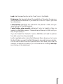
1. INTRODUCTION
1.1 INTRODUCTION
ReDSPider is a TDM plug-in library that allows the user to load sound processing devices from a complete list. As a result, unique and exciting new
effects can be created with just one product.
A large library of presets is provided as standard, and will be permanently
updated.
The user can modify and automate most of the parameters which control the
modules, which are the basis of the internal plug-in structure.
9
1.2 INSTALLING REDSPIDER
Please read the TDM Install Instructions that are located in the master
Installer disk (the disk with the serial Number)
10
1.3 DSPIDER AND REDSPIDER
The use of ReDSPider is as easy as loading standard presets, most of whose
parameters can then be modified. To satisfy all our customers’ requirements
we have implemented two products: DSPider and ReDSPider. The first
allows to create the patches which can be loaded from ReDSPider, which is
reserved to “load” those patches (and to save the settings). All patches
loaded with ReDSPider have been created with DSPider. You cannot change
the internal structure of the plug-ins with ReDSPider, as this feature is
reserved for DSPider.
The loadable plug-ins can be DUY presets, third party presets or DSPider
users’ creations.
You must bear in mind that with ReDSPider you can modify control values
and other bypass/mute parameters, but no access to the internal structure of
the plug-in patch is possible.
ReDSPider includes as standard a long list of plug-ins which will be enlarged
and updated regularly. These enable you to use this plug-in as a compressor,
limiter, reverb, stereoizer, enhancer, maximizer, panner... or as a
combination of them by using multiple insertions in a same track.
11
12
2. STARTING OUT WITH REDSPIDER
2.1 INTRODUCTION
ReDSPider is designed for loading plug-in patches, allowing you to modify
and save all the control changes you make, but without modifying the
internal structure and functions of the plug-in.
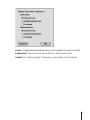
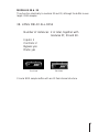
To insert ReDSPider in your track, simply select it from the list of plug-ins
in your sequencer. In this list of plug-ins, with all your others, you will see
the following ReDSPider options:
In a mono track:
ReDSPider (mono)
ReDSPider (mono/stereo)
In a Stereo track:
ReDSPider (stereo)
The 3 available ReDSPider modes are ReDSPider (mono), ReDSPider
(mono/stereo) and ReDSPider (stereo).
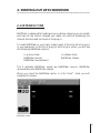
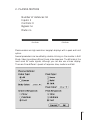
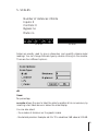
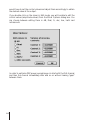
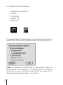
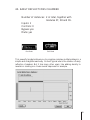
When you insert the ReDSPider option in a Pro Tools™ track you will
visualize this screen:
ReDSPider Screen
13
This is the standard screen for ReDSPider. You will see that it is split into
two sections. The left side includes the save/load controls –among others-,
and will be referred to as the "palette" from now on in this manual.
The right side of the screen is the surface where the plug-in modules and
controls will appear. This part will be called the "Blackboard".
Inside the "Blackboard" you will usually see graphical modules: sliders,
plasma displays, scopes, text and numeric readouts (please refer to chapter
3 for a detailed description of these modules). This is because these are the
modules you use most often to control values and observe the results.
However, many more modules than these are used to create the internal
structure of the plug-in patch with DSPider. The person who designed the
patch may let you visualize some of these other modules on the screen so
that you can change their parameters.
For example, in certain cases you may want to use the mute and bypass
features which are available on most modules, in order to create specific
effects. In this case the plug-in designer can make these available to the user
by displaying them.
14
2.2 LEFT SIDE OF THE SCREEN: THE PALETTE
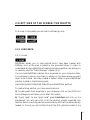
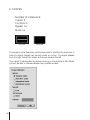
At the top of the palette you will see the following icons:
2.2.1 LOAD/SAVE:
2.2.1.1 Load:
ReDSPider allows you to load patches which have been created with
DSPider, such as the ones included in the provided library. In order to
understand all the possibilities of loading and saving patches, we advise you
to carefully read the “Patch Manager” chapter (2.5).
You can load ReDSPider patches from anywhere on your computer disks.
You just have to save or copy them in advance in the place where you want
them to be located. We have created a default folder to place ReDSPider
patches, located in the following path:
Hard Disk/System folder/DAE folder/Plug-ins/ReDSPider patches
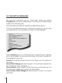
To load existing patches, you have several options:
a) To load a patch from anywhere in your computer, click on the LOAD icon
and a dialog box will allow you to select its location.
b) "Quick load": to use "quick load" press Cmd+Opt and click on the
blackboard. You will see a list of all the existing presets organized into
families. Select one of the patches inside a family and it will be automatically
loaded. In the list you will initially find all the DUY patches located in the
15
default folder, but you can also add your own patches, third parties’ patches,
or future new DUY patches to the list. We have initially created some
standard families of patches, which will make it easier to find the desired
patch but you can also add your own families. The maximum number of
patches that can be selected in this way is limited to 256. These patches can
be held inside folders. The maximum number of folders is unlimited, but
you may want to keep it much lower than 256 for practical purposes. Only
one level of folders is allowed. Hence you can not put a folder inside another
folder. If you do so the "quick load" feature will not work properly.
c) Using the Patch Manager. This feature is explained in chapter 2.5.
2.2.1.2. Save:
Clicking on this icon will allow you to save whichever control changes you
have made to the patches you previously loaded. You can also use the Pro
Tools option to save patches via the mini-menu located at the top of the
plug-in window.
The patch files used with ReDSPider are identical and compatible with the
ones in the full version of DSPider.
We advise you to create a specific folder to save your settings. You may avoid
confusion by having a properly structured group of folders.
Let's say you load one of the Compressor presets. You will see a few
parameters which you can modify, such as ratio, attack, release and
threshold (although there may be many more). You may also have a Shift
Left module with a label above indicating that this module adds a 6dB gain.
In this case, you would also be able to see that module on the screen. Once
you have modified values on the patch, you can save it as a new preset.
16
2.2.1.3. The Patch Manager. Saving your patches for "quick-load" and
Cache Management.
ReDSPider allows you to choose the root folder where you want to load your
patches from when using “quick-load”. This new feature is called the “Patch
Manager”.
When you “quick-load” patches for the first time by holding Cmd+Opt and
clicking on the Blackboard ReDSPider will take you to a default folder
located in the following path:
Hard Disk/System folder/DAE folder/Plug-ins/ReDSPider patches
You will visualize the list of patches which can be loaded at this location.
However, you can choose the path where to load and save your patches for
“quick-load”. We will get to that point a little later.
The Patch Manager is used via a menu located at the top of the patch list
which appears when clicking on the Blackboard while holding Cmd+Opt.
Its functions are:
Save as: Has exactly the same function as the “Save” icon at the bottom of
the Palette. You choose a location where to save your patches, totally
independent of the root folder for “quick load”.
Save in Patch Manager as: saves the patch in the root folder selected from
the “preferences” menu (see the “preferences” description below).
Save Locked as: Saves the patch locked (the structure of the patch will not
be visible when loaded and no edition will be possible).
Save Locked in Patch Manager as: Saves the patch locked in the chosen root
folder.
Load: Has the same function as the “Load” icon in the Palette.
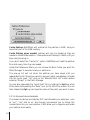
Preferences: We have introduced the possibility of choosing the way you
use the cache with ReDSPider. If you select the “Cache On” option, you have
two alternatives:
17
Cache Patches: ReDSPider will preload all the patches in RAM, using an
important part of the DAE memory.
Cache Patches when needed: patches will only be loaded as they are
needed in a ReDSPider session. These patches will be kept in RAM until you
stop using the plug-in.
If you don’t select the “Cache On” option, ReDSPider will read the patches
from disk every time they are loaded.
Inside the Preferences Menu you can choose the Root Folder you want the
Patch Manager to save and load your patches in.
The pop-up list will not show the patches you have saved until you
regenerate the list. Should you want to see your patch immediately included
into the "quick load " list, click on the “Rebuild Patch List” button before
pressing “Accept” in the Patch Manager.
You can also regenerate the "quick-load" list, by holding the Opt key while
at the same time pressing the "Save" icon on the left of the screen. You can
then release the Opt key and type the name of the patch you want to save.
2.2.1.4 Nomenclature standards.
The names of patches provided by DUY are followed by an extension, such
as “.pci”, “.ms” and so on. We strongly recommend you to follow this
nomenclature for your own patches. It will allow you to organize and locate
your patches more easily.
18
The possible extensions are the following:
.mm
.ms
.ss
.pci
.mix
for patches with a mono input and a mono output.
for patches with a mono input and a stereo output.
for patches with a stereo input and output
use this extension if the patch is not compatible with the
Nu-bus DSP Farm
use this extension if the patch has been optimized for the MIX
system
2.2.2 REDSPIDER PATCH-CORD VIEWS
If the designer of the patch decided to let you see the patchcords that
connect one module with another, the loaded preset may have several
modules included on the display surface, with several connections that may
seem confusing. To avoid this problem we have introduced two ways of
visualizing connections: 90 Degree View and Direct View.
2.2.2.1. 90 Degree View:
In 90 Degree View mode all patch cords are connected forming 90 degree
horizontal or vertical angle paths. This mode gives you a very clean and tidy
display surface.
2.2.2.2 Direct view:
The Direct View connects modules with straight lines between modules.
Direct view may look confusing at first, but makes it very easy to see the
source and destination of a patch cord.
19
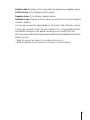
2.2.3 INSTANT HELP
Three icons below the Save/Load icons on the palette provide help to the
user while working with ReDSPider.
2.2.3.1 Patch information
Click on this icon and a dialog box will appear on the screen showing
information about the current patch. Please note that only previously
created patches on disk can read and modify this information.
2.2.3.2 Balloon Help
By clicking on this icon you will switch the help mode on or off. This
provides you with help on whichever module your mouse is placed over, on
the Blackboard surface or on the Palette. To switch between the active or
inactive status of Help, simply click on the icon.
2.2.3.3 Talking Help
By clicking on this icon, the Speech Manager will read the text given in the
Help Balloons. In order to get talking help, you must have the Speech
Manager installed in your system.
To switch between the active or inactive status of Talking Help, simply click
on the icon.
20
2.3. RIGHT SIDE OF THE SCREEN: THE "BLACKBOARD"
Within the "Blackboard" you have access to all the parameters that the
designer of the plug-in chose you to see. The designer did this with the full
version of DSPider.
The modules which you will see most of the time in Reader mode are the
graphical modules: sliders, plasma meters, scales, scopes, text and numeric
readouts.
There is more information about them in the Modules section of this manual
(chapter 3).
Some modules can be muted and/or bypassed. These two functions are
explained in points 2.3.1 and 2.3.2.
21
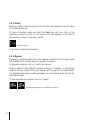
2.3.1 Mute:
Muting a certain module means that its output will always be a zero value
in the digital domain.
To mute a module, press and hold the Cmd key until you click on the
module you want to mute. In this case, a cross will appear on the right of
the module to show it has been muted.
Muted multiplier
To unmute, repeat the procedure.
2.3.2 Bypass:
Bypassing a module means the output signal is identical to the input signal
and therefore the module does not modify the signal.
To bypass a module, click on it with the mouse.
Some modules have different bypass positions. Example: a subtraction
module has two inputs (the input signal and the signal to be subtracted).
You therefore have two possible bypasses: the input signal and/or the to-besubtracted signal.
To stop bypassing a module, click on it again.
Possible bypass positions of a subtraction module.
22
2.4 USING REDSPIDER WITH THE PRO TOOLS|24 MIX CARD
This version of ReDSPider is optimized for the Pro Tools|24 MIX card and is
compatible with the PCI system.
MIX users can take advantage of the increase of the maximum number of
instances for certain modules. Please note this increase is only available for
MIX users. If you own a PCI system you will find the number of instances
for each module as specified in their detailed explanation in chapter 3 of the
User’s Manual.
The maximum number of instances for sliders, mixers and short, medium
and long delay modules is doubled compared to the PCI system. Therefore,
with the MIX system you can insert a maximum of 32 sliders, 8 mixers, 14
short delays, 6 medium delays and 4 long delays.
23
2.5 THE PATCH MANAGER
We previously mentioned you can “quick-load” patches by holding
Cmd+Opt and clicking on the Blackboard. This takes you to a default folder
located in the following path:
Hard Disk/System folder/DAE folder/Plug-ins/ReDSPider patches
One of the new features allows you to select the root folder you want to load
your patches from. This new feature is called the “Patch Manager”.
Press Cmd+Opt and click on the Blackboard to visualize the list of patches
which can be loaded. You will see an extra menu at the top of the patch list.
The available functions are:
Save as: Does exactly the same function as the “Save” icon at the bottom of
the Palette.
Save in Patch Manager as: Saves the patch in the root folder selected from
the “preferences” menu (see below).
Save Locked as: Saves the patch locked (the structure of the patch will not
be visible when loaded and no edition will be possible).
Save Locked in Patch Manager as: Saves the patch locked in the chosen
root folder.
24
Load: Has the same function as the “Load” icon in the Palette.
Preferences: We have introduced the possibility of choosing the way you
use the cache with ReDSPider. If you select the “Cache On” option, you have
two alternatives:
Cache Patches: ReDSPider will preload all the patches in RAM, using an
important part of the DAE memory.
Cache Patches when needed: patches will only be loaded as they are
needed in a ReDSPider session. These patches will be kept in RAM until you
stop using the plug-in.
If you don’t select the “Cache On” option, ReDSPider will read the patches
from disk every time they are loaded.
Another available option inside the Preferences Menu allows you to choose
the Root Folder you want the Patch Manager to save and load your patches.
You can also re-build the list of patches, which will allow you to see the
names of the patches included in your root folder when holding Cmd+Opt
and clicking on the blackboard.
25
26
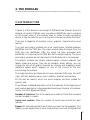
3. THE MODULES
3.1 INTRODUCTION
Chapter 3 of this Manual is an excerpt of DSPider’s User Manual. Since the
designer of a patch (DSPider user) may allow a ReDSPider user to visualize
on the screen some of the modules used to create a certain processing
device, it may be useful for you to know which are each module’s functions.
There are 4 categories of modules: in/out, graphics, single functions and
macros.
The input and output modules act as an input/output interface between
ReDSPider and the TDM Bus. The input module takes the signal from the
TDM Bus into ReDSPider. After the signal has been processed with
ReDSPider, it is returned to the TDM Bus via the output module. The input
and output modules are not described in the Modules list in this manual.
The graphic modules are: sliders, plasma meters, numeric readouts, text
labels, scales and scopes. They are all resizable. When editing, you can
change the size of all graphic modules by clicking and dragging a small
red/white square which appears on one of the corners of the box
surrounding the module.
The single functions are those which have a standard DSP code, like shift
right, shift left, absolute value, invert, addition, subtract and multiply.
All the rest are macros, which are more complex functions created for
specific uses.
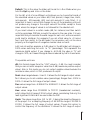
There follows a detailed description of all the modules. At the beginning of
each module description a few parameters are shown: Number of instances,
Inputs, Controls, Bypass and Mute.
Number of instances: This is the maximum number of times that a module
can be included in a patch.
Inputs and controls: State the number of inputs and controls for each
module.
Bypass: All the modules that have at least one input can be bypassed. This
means you can bypass them in such a way that you can hear the signals that
27
enter each module individually and one by one. To bypass a module you
just have to click on it in Run mode. The module will toggle between the
different inputs and operating positions.
Mute: All the Single function and Macro modules can be muted. To do so,
click on the module while at the same time holding the Cmd key. An "x"
symbol will appear indicating that the module has been muted.
Modules can have a minimum of one visible output lead when visible. This
output, when available, can be tied to an infinite number of inputs. So we
can say that all the following modules have infinite outputs: the single
functions, all the macros, the input modules and the sliders. Plasma meters,
however, have only got one output, which is prepared to be patched to a
numeric readout module.
3.1.1 DSPider: Run, Edit, Advanced and Reader Modes
DSPider is divided into two sections/modes: Advanced and Reader.
Reader Mode: Is equivalent in use to ReDSPider, and allows to read patches
but not modify their internal structure.
Advanced Mode: This mode has a bigger display screen than Reader Mode
and includes all the modules on the palette which can be “dragged &
dropped” onto the blackboard and patched between them, creating the
internal structure of the plug-in. There are two ways to use this mode: Run
and Edit Mode. It’s in the second that you can edit the module’s parameters
and the internal structure of those plug-ins which are not locked.
It is important that you have understood these last concepts before reading
any further.
28
3.2 Module list
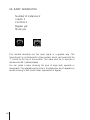
1- SLIDER
Number of instances: 16
Inputs: 0
Controls: 0
Bypass: no
Mute: no
Run Mode
Edit Mode
A slider generates a digital value proportional to its position. It can be used
to generate control settings for most of the functions available to the user (in
reader mode) and also to generate constants, generally not available to the
user. This is made possible by the multiple programmable parameters
available in Edit Mode. You can enter Edit Mode by double clicking on the
slider. A dialog box with several settings will appear:
29
On the right side of the box you can set four values:
Minimum: this is the value your slider will reach in Run Mode when it is
totally to the left horizontally or completely down when being used in a
vertical position.
Maximum: The value assigned when the slider is completely to the right in
Run Mode (or at the highest position if the slider is oriented vertically). It is
important for you to bear in mind that the Minimum value will always
correspond to the left of the slider (or down vertically) even if the entered
minimum value is higher than the maximum. Therefore, you can set a
lower value for the Maximum than for the Minimum, in which case you
would have the smaller value at the right (or at the top according to the
orientation).
Current: This indicates the last value the slider was set to when you last quit
Run Mode. If you change it, the new settings will apply.
30
Default: This is the value the slider will be set to in Run Mode when you
hold the Opt key and click on the slider.
On the left, a list of nine different units allows you to choose the format of
the visualized values on your slider: dB, Float, percent, integer, Hex, Hertz,
mili-seconds, Mili-seconds (AR) and mili-seconds (2 pole filter). It is
important to bear in mind that changes to any of the preceding units will
not produce any change in the output value of the slider, except in those
cases where the range of values is not allowed for the selected unit.
If you insert values in a certain mode (dB, for instance) and then switch
units to percentage, DSPider converts the values to the new scale. It is very
important that you consider the valid ranges for each unit, as the conversion
could lead to mistakes. For example if you set a float value to -4 (minus
four) and then switch to the dB mode, the conversion will not be done
properly, as the logarithm of a negative number does not exist.
Let's look at another example: a 0 dB value (in the dB scale) will change to
100% when switching the units to "%" (percentage). This represents the
maximum digital output. If you change to -6.02 dB, the value in "%" will
change to 50%, as it means the signal value is reduced by half in linear terms.
The possible units are:
dB: this format ranges from the "-INF" value to 0 dB. You must consider
that you can not enter a superior value than 0 dB (maximum positive output
value). Also in this mode you can not output negative values because the
minimum value, which is -INF produces a 0 output
float: values range between -1 and 1. It allows the full range of output values.
%: it allows you to set a relative value (percentage). Ranges from -100% to
100%. It allows the full range of output values.
Dec: values range from -8.388.607 to 8.388.607. It allows the full range of
output values.
Hex: values range from FF800001 to 7FFFFF (hexadecimal numbers),
which allow the full range of 32-bit output values, considering that only the
least significant 24 bits will be used inside the DSP.
Hertz: The values range from -S/2 to S/2 , S being the sampling frequency
of the project. For a sampling frequency of 44.100 the range is -22.050 to
22.050. It allows the full range of output values. Choose this option to
control the frequency of the oscillators. It allows the full range of output
31
values. However, to control oscillators you can't use negative values. Do not
use this unit for controlling filters, as a different unit was created for this
purpose.
Mili-seconds: This mode was designed to control the delay modules and
gives a direct conversion from samples (if set in Integer mode) to miliseconds. The values range from -8.388.607/S to 8.388.607/S, where S is the
sampling frequency in KHz. For a 44.1 KHz sampling frequency the range
will be -190.217 to 190.217 seconds. Even in a range of more than 380
seconds the useful range is limited to the size of the delay. For the three
types of delays (S, M or L) the useful range is for positive values up to
2047/S, 4095/S and 8192/S, which for a sampling rate of 44.1 KHz will be
around 46, 92 or 185 ms. One sample delay at this frequency is 0.22676
miliseconds long. Please refer to the delay modules for more details
(modules 30 to 39)
Mili-seconds (AR): This unit is used to control the attack and release values
of envelope followers and ramp generators. Although negative values are
allowed, they are not useful for controlling attack and release parameters.
The practical values range from INF to 1/S, S being the sampling rate in
KHz. For a sampling rate of 44.1 KHz the range will be INF to 0.022676
ms. Please refer to modules 26 and 28 for more details (Ramp generator and
Envelope follower modules)
Hertz (2 Pole Filters): Choose this option to control the frequency of the
two pole filters (modules 18 to 21). The values range from -7577.3 to
7577.3 Hz. We advise you only to use positive values to control filters. The
useful range is 20 to 7577.3 Hz. Do not use this unit for controlling
oscillators.
The tracking option allows you to select the curve that relates the output
values to the slider position when using the slider in Run mode. You can
choose between three different options: Linear, dB and AR. Linear and dB
are self explanatory. The AR option is optimized for controlling attack and
release times.
The Templates section provides a fast way to set all the Slider Options values
for most typical uses. The predefined templates are: Gain, Filter, Oscillator,
LFO, AR (Attack and Release), and Short, Medium and Long delays.
When using the slider in Run or Reader Mode, you can fine-tune when
choosing a value with the slider by pressing Cmd while changing the value
on the slider with the mouse.
32
2- PLASMA METERS
Number of instances: 16
Inputs: 1
Controls: 0
Bypass: no
Mute: no
Run Mode
Edit Mode
Plasma meters are high-resolution bargraph displays with a peak and hold
option.
Several parameters can be edited by double clicking on the module in Edit
Mode. Value type allows dB and linear scale responses. The dB scale is the
most usual for audio signals, although you can also use a linear display.
There are three different speeds of response: slow, medium and fast.
33
You can also have a peak display on the plasma meter, which is a small mark
on the maximum achieved value. You can choose between three different
modes:
None: does not display a peak value.
Hold: displays and holds the maximum value during a period determined
by the Peak Response time (slow, medium or fast).
Shift: displaces (moves) the peak display according to the peak signal, and
then falls more slowly with speed defined by the Peak Response time: slow,
medium or fast.
Both the bargraph and the peak display have different color options: blue,
silver, magenta, red, yellow and green.
Plasma meters are usually combined with a scale module, although this is
not obligatory.
34
3- NUMERIC READOUT
Number of instances: 32
Inputs: 1
Controls: 0
Bypass: no
Mute: no
Run Mode
Edit Mode
This module is used to display values in a numeric form. When editing
(double click on the module in Edit Mode) you can choose the units which
will be used for display: dB, Float, Integer, Hex, %, Hz, kHz, Seconds, MiliSeconds, Seconds (AR), Hz (2 Pole Filter) and KHz (2 Pole Filter). The
ranges of these units are equivalent to the ones explained in the Slider
module section.
35
dB: Displays values in decibels (range from "-INF" to 0 dB). Please note
that values above 0 dB are not allowed.
float: values are float numbers ranging from -1 to 1.
integer: displays values as integer numbers ranging from -8.388.607 to
8.388.607.
Hex: displays hexadecimal values ranging from FF800001 to 7FFFFF. It
allows the full range of output values.
%: it allows you to visualize a relative value (percentage). It ranges from 100% to 100%.
Hertz: choose this option to read the frequency of oscillators. This is not a
suitable option for filters. Values range from -22050 to 22050. However for
oscillators you will not use negative values.
KHz: Used in the same way as the Hertz option, it displays frequency in
kilohertz.
Seconds: This mode was designed for the delay modules. It gives a direct
reading in seconds.
Mili-seconds. This mode was designed for the delay modules. It gives a
direct reading in mili-seconds
Seconds (AR): This unit is used to measure the attack and release values of
envelope followers and slope modules. It gives a direct reading in seconds.
Mili-seconds (AR): Also measures the attack and release values of envelope
followers and slope modules. It gives a direct reading in mili-seconds
Hertz (2 Pole Filter): Choose this option to visualize the frequency of the
2 pole filters (modules 18 to 21). You can also optionally control 1 pole
filters (modules 16 and 17).
Kilohertz (2 Pole Filter): The same as the previous option but scaled in
kilohertz.
You have more visualization options: Decimal Places, Display Unit, Hold
Peak Value, Display Box, and the Templates.
Decimal Places: You can select the number of decimal places you want the
readout to display and thus the precision of the reading. In the "fine mode"
(Cmd-drag) the graphical resolution also depends on this setting.
36
If you had a -32 dB value to display and you chose a dB type with 2 decimal
places you would visualize "-32.00 dB" to "-32.99" on the display box,
therefore increasing the resolution. In this case the readings would be in
steps of 0.01.
Display unit: It allows you to display the unit (dB, float, Hz and so on) next
to the value when in Run Mode.
Hold Peak Value: the readout displays the maximum value reading. If you
choose this option, you may want to reset the counter to find a new peak
value when you're working in Run Mode (or in Reader Mode). To do so,
simply click the module in Run Mode.
Display box: select if you want to see a small box enclosing the measured
value.
As with the Slider module the Templates section provides a fast way to set
all the Plasma Meter Options providing the most typical settings for certain
uses. The predefined templates are: Gain, Filter, Oscillator, LFO, AR (Attack
and release), and Delays.
It is important to note that the numeric readouts can not be patched from
any module output. In fact they can only be patched from a Slider module
and to a Plasma Meter.
If you need to patch a Numeric Readout to another kind of module we
recommend inserting one Plasma Meter as a bridge.
37
4- TEXT LABELS
Number of instances: infinite
Inputs: 0
Controls: 0
Bypass: no
Mute: no
Run Mode
Edit Mode
To insert a text label, simply drag the module onto the blackboard and
double click in Edit Mode. Insert the text into the dialog box and you will
be able to visualize it when you go back to Run Mode. We advise you to
label all the patches you create as well as some of the modifiable parameters
to keep a good record of all the controls you create on your DSPider patch.
You can also draw squares in order to enclose specific areas of the
blackboard. These squares can also have text in them.
To create a square make sure you are in Edit Mode. First, double click on
the module, write a text if you wish, and activate the Draw Frame option.
Press OK. Still in Edit Mode, you will see a red or white small square on the
lower right corner of the label box. By clicking and holding while dragging
you can enlarge the surface to which the label is extended. The labelled
square will be present in Run and Reader modes.
38
5- SCALES
Number of instances: infinite
Inputs: 0
Controls: 0
Bypass: no
Mute: no
Run Mode
Edit Mode
Scales are usually used to give a dimension and quantify plasma meter
readings. You can change the scale type by double clicking on the module.
There are four different options:
dB
linear
%: percentage
no scale: allows the user to label the scale he prefers at his convenience, by
inserting a text label above or below the scale display.
You can also select:
- the number of divisions on the graphic scales
- the decimal precision. Example: set it to '2' to visualize a 3 dB value as 3.00 dB.
39
6- SCOPES
Number of instances: 4
Inputs: 1
Controls: 0
Bypass: no
Mute: no
Run Mode
Edit Mode
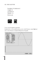
The scope is a low frequency oscilloscope used to visualize the evolution in
time of a signal. Signals can be both audio or control. The signal appears
from the right side of the screen and moves towards the left.
If you enter the dialog box by double clicking on the module in Edit Mode,
you will be able to choose between four possible modes:
40
Double Lobe: Displays on the scope both the positive and negative values.
Positive Lobe: Only displays positive values.
Negative Lobe: Only displays negative values.
Absolute Lobe: Displays positive values as positive but converts negative
values to positive.
You can also choose the signal speed on the screen (Fast, Normal or Slow).
Finally, you can select a color for your display. Click on the predefined color
and another dialog box will appear allowing you to modify the color.
When you are visualizing the signal (and therefore using the Reader Mode or Run
Mode), you can:
- Reset the screen and clean it, by double clicking on it.
- Hold the display on the screen, by clicking on it and holding.
41
7- SHIFT RIGHT
Number of instances: 12 in total together with shift
left modules
Inputs: 1
Controls: 0
Bypass: yes
Mute: yes
Run Mode
Edit Mode
The shift right module reduces the input signal by half. The equivalent reduction
in dBs is -6.02 dB.
42
8- SHIFT LEFT
Number of instances: 12 in total together with shift
right modules
Inputs: 1
Controls: 0
Bypass: yes
Mute: yes
Run Mode
Edit Mode
Shift left doubles the input signal. That is it increases its level by 6.02 dB.
Note that shift left can lead to clipping distortion, if not properly used.
43
9- ABSOLUTE VALUE
Number of instances: 6
Inputs: 1
Controls: 0
Bypass: yes
Mute: yes
Run Mode
Edit Mode
The absolute value function converts all negative input values to positive,
leaving all positive values the same.
A "-5" value would be turned to "+5", and a "+6" level would remain
untouched.
44
10- INVERT
Number of instances: 6
Inputs: 1
Controls: 0
Bypass: yes
Mute: yes
Run Mode
Edit Mode
The invert module multiplies the entered signal by "-1". This is equivalent
to a 180 degree phase change.
45
11- ADDITION (and logical operator)
Number of instances: 16 together with subtraction
and multiplication modules
Inputs: 2
Controls: 0
Bypass: yes
Mute: yes
Run Mode
Edit Mode
This module takes the inserted signals A and B and adds them (A+B),
although you can also use this module as a logical operator for OR, AND
and XOR ("exclusive OR") functions and even as a switch.
In order to choose the operation you want the addition operator to process,
double click on the module in Edit Mode. You can then select the operation
(ADD, OR, AND or XOR).
A
0
1
0
1
B
0
0
1
1
OR Out
0
1
1
1
AND Out
0
0
0
1
XOR Out
0
1
1
0
You can activate the "Intelligent Polarity" box to avoid problems with signed
signals.
46
The "Missing Input (2) Value" box allows you to set a value for the second
input without the need to connect an external signal. This is suitable for all
those cases in which one of the inputs remains constant.
These logical functions are very useful for creating certain kinds of
distortion effects, as well as dithering.
You can also use this module as a 2-state switch. When using this option,
the module will act as a two-state bypass between inputs A and B. In this
case you will visualize the addition icon bypassed on the blackboard. The
missing value, which can be modified in the module's edition dialog box, is
still relevant, since it is easy to create a Bypass/Mute function by making the
missing value zero and not connecting the second input. On the other
hand, if we have to complete sections of DSP, we can select one or another
by connecting both sections to both module inputs and selecting the 2-state
switch option.
47
12- SUBTRACTION
Number of instances: 16 in total together with addition
and multiplication modules
Inputs: 2
Controls: 0
Bypass: yes
Mute: yes
Run Mode
Edit Mode
The SUBTRACTION module subtracts the value of the second input from
the first. If you insert signals A to the first input and B to the second, the
result will be A-B.
Please remember that the signal to be subtracted must be inserted into the
second input, as can be seen in the figure above.
48
13- MULTIPLICATION
Number of instances: 16 in total with addition and
subtraction modules
Inputs: 2
Controls: 0
Bypass: yes
Mute: yes
Run Mode
Edit Mode
This module is used to multiply or divide two signals.
Double click on the module in Edit mode and you will be able to choose
between several options:
49
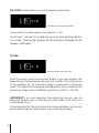
MULTIPLY: Use this option to use the module as a multiplier.
Multiplier functioning as a multiplier
Inverse result: The result given by the module is -A*B
Round result: The result is rounded, taking out the least significant 24 bits.
Low 24 Bits: Takes the least significant 24 bits as the result. Remember that the
operation is 48-bit wide.
DIVIDE:
Multiplier functioning as a divider
Select this option to use the module as a divider. If you insert signals A and
B according to the figure below, the result will be (A:B). This is the division
of one quadrant for non-fractionary integer numbers with a fractionary
result. This means that, for example, dividing number 20 by number 40 will
produce an integer value of 4194304, equivalent to a 50% or -6.02 dB.
IMPORTANT!: You must remember that dividing by zero will give the
maximum possible value in that scale as a result (0dB in dB, 100% as a
percentage and so on)
It's also important for the user to know that using a multiplier is not the only
way to amplify signals. There are four ways of amplifying signals:
50
a) Using a shift left module, which increases the original value by 6.02 dB.
b) To create the same effect as the above mentioned, you can insert the same
signal into both signal inputs of an Addition module. The resulting signal is
exactly twice the original signal, which corresponds to +6.02 dB.
c) You can also amplify a signal by inserting it into a MIXER several times
(see module number 24 for complete information) and controlling the
values with the use of sliders as gain controllers or by setting the values in
the mixer dialog box. Mixers have four inputs, which means the maximum
amplification you can achieve is +12.04 dB. This corresponds to inserting
the signal in every channel of the mixer with a 0dB attenuation.
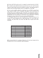
In the diagram below we can see the amplification values according to the
number of channels added with an 0dB attenuation (for more than four
channels, use more than one mixer and add their outputs with ADD
modules):
Number of channels at 0dB att. Amplification
2
6.02 dB
3
9.54 dB
4
12.04 dB
5
13.98 dB
6
15.56 dB
7
16.90 dB
8
18.06 dB
d) By using dividers: for example dividing by 0.5 the input signal will be
doubled (this is only the case with positive signals)
51
14- NOISE GENERATOR
Number of instances: 1
Inputs: 0
Controls: 1
Bypass: no
Mute: yes
Run Mode
Edit Mode
This module is a pseudo-random white noise generator.
This module has no input signal, as it's a stand-alone generator. The
amplitude of the noise signal can be set by the control input. One possible
way to do so is by inserting a slider into the amplitude input controller to
specify the level.
52
15- SAMPLE & HOLD
Number of instances: 2
Inputs: 1
Controls: 1
Outputs: infinite
Bypass: yes
Mute: yes
Run Mode
Edit Mode
This module performs the "sample and hold" function widely used by
synthesizers in the analogue world.
The S&H module stores the input signal in memory during a period of time
specified with the control input, preferably a slider. Please remember that
the value must be set in seconds or miliseconds.
53
16- ONE-POLE LOW-PASS FILTER
Number of instances: 8 in total together with one-pole
high-pass filters.
Inputs: 1
Controls: 1
Bypass: yes
Mute: yes
Run Mode
Edit Mode
This filter has a -6dB/octave slope beginning at the cutoff frequency stated
with the control input at the top of the module, marked with a "C" (which
stands for 'cutoff'). This frequency can be specified with a slider.
One-pole filters are very useful for shelving equalization and other gentle
processing functions.
54
17- ONE-POLE HIGH-PASS FILTER
Number of instances: 8 in total together with one-pole
low-pass filters.
Inputs: 1
Controls: 1
Bypass: yes
Mute: yes
Run Mode
Edit Mode
The one-pole high-pass filter has a -6dB/ octave slope leading to the
specified frequency (adjust with a slider) and then remains constant at a 0dB
gain level towards the high spectrum frequencies. There is a gentle
transition around the cutoff point. (Please read the one-pole low-pass filter
specifications).
55
18- TWO-POLE LOW-PASS FILTER
Number of instances: 8 in total together with the rest
of two-pole filters.
Inputs: 1
Controls: 2
Bypass: yes
Mute: yes
Run Mode
Edit Mode
Two-pole low-pass filters have a -12 dB/octave slope starting at the cutoff
frequency, which can be controlled -for instance- with a slider. You can
visualize the frequency you have selected with the slider by connecting a
"Numeric Readout" module and setting it in Hertz or kilohertz.
Two-pole filters have a second control which allows adjustment of the Q
factor, which is a resonance parameter. This value indicates the width of the
peak around the cutoff frequency. When adjusting it, you should consider
that analogue values are not equal to digital values, and therefore a typical
0.5 Q factor in the analogue world would not correspond identically to that
in the digital domain.
Remember that you can either control the Q value with a slider or with an
external signal, which can be obtained from a module. In such a case, it's
important that you insert an absolute value module between the module
you're taking the signal from and the point to which you are going to insert
the Q value, at the top of the two-pole filter. This is fundamental, as a
negative value Q makes no physical sense. Therefore, only a positive value
is valid in controlling the Q factor.
56
19- TWO-POLE HIGH-PASS FILTER
Number of instances: 8 in total together with the rest
of two-pole filters.
Inputs: 1
Controls: 2
Bypass: yes
Mute: yes
Run Mode
Edit Mode
Two-pole high-pass filters have a -12 dB/octave slope which turns to a
constant 0dB as it approaches the cut-off frequency (the Q factor, which is
controlled by the user, can make the cut-off frequency value move a few Hz
above or below the specified frequency value), and remains at this level
throughout the rest of the spectrum towards the high frequencies. The Q
value indicates the width of the peak around the cutoff frequency.
57
20- TWO-POLE BAND-REJECT FILTER
Number of instances: 8 in total together with the rest
of two-pole filters.
Inputs: 1
Controls: 2
Bypass: yes
Mute: yes
Run Mode
Edit Mode
The band-reject filter allows you to attenuate a range of frequencies, which
are defined with the center frequency value and the Q factor. These two
controls can both be specified with sliders.
The Q factor determines the width of the frequency range to avoid starting
at the frequency value set in the left control. The lower Q value you set, the
narrower the frequency range to be omitted will be. If you choose a very
high value Q, you will be rejecting a wide range of frequencies.
58
21- TWO POLE BAND-PASS FILTER
Number of instances: 8 in total together with the rest
of two-pole filters.
Inputs: 1
Controls: 2
Bypass: yes
Mute: yes
Run Mode
Edit Mode
The two-pole Band-pass filter rejects all frequencies outside the frequency
range selected with both the frequency control and the Q factor. The range
of non-attenuated frequencies will vary according to the value of the Q
factor. For this module, a high Q value will mean you will be attenuating
all frequencies outside a very narrow range around the frequency specified
with the left control (center frequency control). If you choose a low Q value,
you will be letting a wide range of frequencies pass through the filter.
59
22- OSCILLATOR
Number of instances: 2
Inputs: 0
Controls: 2
Bypass: no
Mute: yes
Run Mode
Edit Mode
This is a multi-waveform generator.
Double click on the module when you're in Edit Mode or press Opt and
click in Run Mode. A complete dialog box will appear.
60
On the left you will be able to click on one of the following signals:
Sine
Triangle
Sawtooth
Squarewave
FM.
When you have clicked on your signal choice, a display screen on the right
of the dialog box will show the signal in a time domain. Another screen at
the bottom of the dialog box will display the signal on a frequency scale: the
signal's spectrum.
On the second column at the left of the dialog box you have 5 options:
Amplify: Click to amplify the signal, which is "cut" when surpassing the
limits of the box where the graphic signal is represented (right of the dialog
box).
Reduce: Click here to attenuate the amplitude of the signal.
Invert: Introduces a 180 degree inversion.
DC adj: Allows you to set an offset value for the signal.
Smooth: Reduces high frequency harmonics.
There is also a ratio dialog box and a modulation percentage value which
can be set by the user when generating an FM signal.
Another interesting feature is the possibility to edit the signal frequencially.
Click on the frequency you wish to enhance or diminish and move the
mouse vertically upwards or downwards to achieve an amplification or
reduction of certain harmonics.
The controls at the top of the module are marked with an 'F' and an 'A'. The
first allows you to select the frequency of the signal which is going to be
generated. The values you can choose range from zero to half the sample
rate frequency. The 'A' control lets you change the amplitude.
To draw a DC signal, hold shift while drawing with the mouse on the timedomain window in the dialog box. This will enable you to draw a straight line.
To delete, hold Cmd and drag. You can delete either in the time of frequency
domain windows.
61
23- TRIANGLE OSCILLATOR
Number of instances: 2
Inputs: 0
Controls: 2
Bypass: no
Mute: yes
Run Mode
Edit Mode
This module is a fixed triangular-signal generator. It is very suitable for
LFOs and sound synthesis generation.
The controls at the top of the module are:
'F': it allows you to select the frequency of the triangular signal which is
going to be generated. The values you can choose range from zero to half
the sample rate frequency.
'A': this control lets you change the amplitude.
62
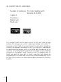
24- MIXER
Number of instances: 4
Inputs: 4
Controls: 4
Bypass: yes
Mute: yes
Run Mode
Edit Mode
The Mixer module is a 4-channel mixer, and therefore has 4 inputs, which
are controlled with the upper controls. You can use a slider for this purpose
or double click to set the values in a dialogue box without needing any
control connections. The four controls allow external control over each
input's gain, but missing controls (those which have not been connected)
will use internal values (which can be programmed in Advanced Mode,
from the Mixer's dialog box).
The mixer allows negative input controls and can therefore be used as a
controllable phase inverter. The negative input controls have the effect of
inverting the input signal. You have to bear in mind that you can not obtain
phase inversion if you are using a slider set to dB units. This is because the
minimum value "-INF" is zero and not a negative value. You have to use
other units for this purpose.
You can also use Mixers as amplifying devices without the need to use shift
left modules. However you can not do this with just one input. For example:
if you want to amplify a signal by 12.04 dB, you would have to introduce
the same signal in the 4 inputs and set the control values to 0 dB. Knowing
that adding two identical signals will increase the original value by 6.02 dB
and repeating the operation for the other two inputs, we will have the
desired value (6.02+6.02=12.04). If we wanted a 10.7 dB amplification we
63
would have to set the control values and adjust them accordingly to obtain
the desired value at the output.
If you double-click on the mixer in Edit mode, you will be able to edit the
control values (amplitude values) from the Mixer Options dialog box. You
can choose between editing them in dB, float, %, dec, hex, hertz and
miliseconds.
In order to optimize DSP power, we advise you to start with the first channel
and then the channel immediately after and so on without leaving "gaps"
between them.
64
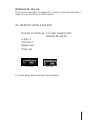
25- PITCH TRACKER
Number of instances: 1
Inputs: 1
Controls: 1
Bypass: yes
Mute: yes
Run Mode
Edit Mode
The pitch tracker module is a period to frequency converter. The output is
a control signal (not an audio signal)
The 'T' control at the top of the module is a threshold parameter which
disables pitch-tracking above the selected value. This threshold is a
frequency threshold, not an amplitude threshold, which means that the
module will not track frequencies above this value.
65
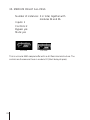
26- RAMP GENERATOR
Number of instances: 2
Inputs: 1
Controls: 1
Bypass: yes
Mute: yes
Run Mode
Edit Mode
This module smoothes out the input signal in a gradual way. This
"smoothness" is controlled with a time constant, which can be set with the
'T' control at the top of the module. This value must be in seconds or
miliseconds (AR ) (attack/release).
You can create a ramp choosing the kind of slope both upwards or
downwards. The selectable options are in the dialog box which appears on
double-clicking in Edit mode: linear, exponential or bypass.
66
Linear: The generated signal between two points is a straight line which joins them.
Exponential: The two points are joined by an exponential curve.
Instant: The resulting signal is formed by joining both points instantly.
67
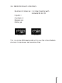
27- SHAPER
Number of instances: 2
Inputs: 1
Controls: 0
Bypass: yes
Mute: yes
Run Mode
Edit Mode
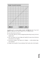
The shaper module is basically a user definable waveshape transformer,
whose X axis represents the original input waveform and Y axis the desired
output.
You can draw the transfer function with 8 linear segments. When you enter
the dialog box (double click in Edit Mode) you will see a 45 degree line
crossing the transfer function axis, meaning the input signal is identical to
the output. To modify this line, simply click and drag the point to draw the
new function curve.
For a quick understanding of how it works, you can see the shaper curve as
a kind of mirror. In linear shaping, illustrated by a straight line in the
diagram, the output mirrors the input waveform exactly. In non-linear
shaping the input meets the line and then reflects a different output
waveform.
68
To delete a point you have already marked, hold Opt and click. If you hold
Shift and drag you will move the point to a 1:1 slope function.
We can draw some conclusions:
1) in the linear case only volume changes are produced by moving the line's
highest point.
2) any curve above the linear shape will amplify the sound and introduce
some kind of non linearity.
3) any abrupt change in the shape, as in diagram...., could produce heavy
non-linearities.
4) shapers can be used for the processing of both audio and control signals.
69
28- ENVELOPE FOLLOWER
Number of instances: 3
Inputs: 1
Controls: 3
Bypass: yes
Mute: yes
Run Mode
Edit Mode
The envelope follower module generates a control signal whose amplitude is
proportional to the input signal amplitude, set by three controls, which are:
Attack: This parameter indicates the time the module takes to respond to
any fluctuations in the input signal. It is usually measured in mili-seconds
(or seconds). So if you control this value with a slider, you should use it in
the AR mode (either miliseconds AR or seconds AR).
70
Release: The 'release' value indicates the length of time throughout which
the signal decay will take place when dropping from a certain amplitude to
a lower value.
Threshold: Set this parameter to set the level above which the module must
be sensitive. During an envelope analysis a signal will not be detected below
this level. If you set a 3dB value, the output from the envelope follower
module would remain constant or decay (according to the release time)
until a 3dB or higher signal was inserted into the module.
Double click on the module in Edit mode. A dialog box will appear,
allowing you to choose between a linear or an exponential follower. This
means that the increase and the decay of the signal follow a linear or an
exponential curve.
The module can also operate as a gate, with either a linear or a quadratic
law. The threshold value determines the triggering value. This gate is opened
and closed according to the attack and release settings previously
mentioned.
71
29- SPECTRAL SHAPER
Number of instances: 2
Inputs: 1
Controls: 0
Bypass: yes
Mute: yes
Run Mode
Edit Mode
This module is a 16-band FFT shaper. Double click on the module in Edit
Mode. You will see the graphic outline of the spectral shape, which corresponds
to an FFT transfer function. Note that the "reset" button allows you to turn all
the values half-way-up in the display box. Therefore, if you wish to amplify
certain frequencies, you just have to click on that bar and without releasing the
mouse make the column higher (or lower if you wish to attenuate).
A very useful application is comb filters.
To delete, press Cmd and drag.
72
30- ONE-SAMPLE DELAY
Number of instances: 8
Inputs: 1
Controls: 0
Bypass: yes
Mute: yes
Run Mode
Edit Mode
This is the simplest of all the delay modules. As its name indicates, it delays
one sample.
73
31- SHORT SAMPLE BUFFER
Number of instances: 7 in total, together with
modules 32 and 33
Inputs: 1
Controls: 1
Bypass: yes
Mute: yes
Run Mode
Edit Mode
This module is a Circular Buffer delay.
The control value determines the delay length. The maximum is 2047
samples.
74
32- SHORT DELAY ALL-PASS
Number of instances: 7 in total, together with
modules 31 and 33.
Inputs: 1
Controls: 2
Bypass: yes
Mute: yes
Run Mode
Edit Mode
This is a circular 2047-sample buffer with an All Pass internal structure.
It has two controls: the first ('D') is a delay value, whose maximum value is
the maximum sample value (2047). The second control ('F') is a feedback
control, which we advise you to set with a slider (for easier use), and
preferably on a percentage scale. This last point is important, since values
between 0% and 50% are stable. When you surpass the 50% value however,
you enter an unstable zone, whose maximum instability depends on the
frequency and is usually around 75%. When you reach the 100% value, the
tendency is to less instability. What you're actually allowing is a great deal
of diffusion, so the sound level may grow and grow. However, values lower
than 50-60 % are very useful for certain applications, which range mainly
from reverbs to other complex processors.
75
33- SHORT DELAY LOW-PASS
Number of instances: 7 in total, together with
modules 31 and 32.
Inputs: 1
Controls: 3
Bypass: yes
Mute: yes
Run Mode
Edit Mode
This low-pass buffer has the same controls as the short delay all-pass
(module 32), although one control is added and labeled with a letter "C"
(viewing it in Run Mode). If you don't connect this last control it performs
in exactly the same way as module 32. But if you connect it, real feedback
is created inside the module, which is controlled with the value set by the
'F' control. The cutoff parameter controls the internal gain in such a way that
it depends on the feedback value. Therefore, to link the Feedback and the
Cutoff you must set them both in such a way that their signals are
complementary. This means that you will have to set the feedback at 75% if
you want a 25% cutoff to the filter’s response. Both parameters must add up
to 100%.
76
MODULES 34, 35 & 36
They function identically to modules 31, 32 and 33, although the buffer is
larger, as it can contain up to 4095 samples.
34- MEDIUM SAMPLE BUFFER
Number of instances: 3 in total, together with
modules 35 and 36.
Inputs: 1
Controls: 1
Bypass: yes
Mute: yes
Run Mode
Edit Mode
A Circular Buffer delay (maximum 4095 samples).
77
35- MEDIUM DELAY ALL-PASS
Number of instances: 3 in total, together with
modules 34 and 36.
Inputs: 1
Controls: 2
Bypass: yes
Mute: yes
Run Mode
Edit Mode
This is a circular 4095 sample buffer with an All Pass internal structure. The
controls are the same as those in module 32 (Short delay all-pass).
78
36- MEDIUM DELAY LOW-PASS
Number of instances: 3 in total, together with
modules 34 and 35.
Inputs: 1
Controls: 3
Bypass: yes
Mute: yes
Run Mode
Edit Mode
This is a circular 4095-sample buffer with a Low Pass internal feedback
structure. It is also known as a Convolution Filter.
79
37- LONG SAMPLE MODULATED BUFFER
Number of instances: 2 in total, together with
modules 38, 39 and 40.
Inputs: 1
Controls: 1
Bypass: yes
Mute: yes
Run Mode
Edit Mode
This is a Circular Buffer delay with modulation. The maximum delay is
8191 samples.
The modulation allows independent control of the delay by means of an
external continuously variable signal. You must use this module in cases
when you need to modulate the delay in real time, without unwanted side
effects. This control is based on the derivative of the modulation signal.
80
MODULES 38 & 39
They function identically to modules 32 and 33, although the buffer is even
larger: 8191 samples.
38- LONG DELAY ALL-PASS
Number of instances: 2 in total, together with
modules 37, 39 and 40.
Inputs: 1
Controls: 2
Bypass: yes
Mute: yes
Run Mode
Edit Mode
Circular 8191 sample buffer with an All Pass internal structure.
81
39- LONG DELAY LOW-PASS
Number of instances: 2 in total, together with
modules 37, 38 and 40.
Inputs: 1
Controls: 3
Bypass: yes
Mute: yes
Run Mode
Edit Mode
Circular 8191-sample buffer with a Low Pass internal feedback structure.
82
40- EARLY REFLECTIONS CHAMBER
Number of instances: 2 in total, together with
modules 37, 38 and 39.
Inputs: 1
Controls: 0
Bypass: yes
Mute: yes
Run Mode
Edit Mode
This powerful module allows you to program complex multiple delays in a
simple and straightforward way. Its most typical use is the creation of early
reflection chambers. But it has many other users, like adding density to
reverbs or creating non linear reverb responses for example.
83
Double click on the module in Edit Mode or press Opt and click on the
module in Run Mode to enter the Early Reflections Chamber's graphic
edition screen. A vertical bar at the left allows you to adjust amplitude
values on a percentage scale. A horizontal bar at the bottom enables you to
mark the length of the early reflection effect (timewise). You are therefore
selecting the room size. To edit these two bars, click and drag with the
mouse and adjust.
Then draw the reflections with the mouse. The maximum number you can
draw is 32. You have to bear in mind that every delay that you program uses
DSP resources, regardless of its amplitude. If you run out of DSP time we
advise you to leave the higher amplitude reflections and remove the low
level ones.
To insert reflections in prime number positions, press Opt while clicking
with the mouse.
To delete certain reflections, hold Cmd while dragging over the reflections
to be erased.
84
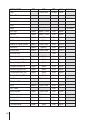
3.3 Quick-keys on modules
The table on the next two pages indicates all possible shortcuts with quickkeys. Please consider the following remarks:
1- The blank spaces indicate no functions.
2- A “bypass” function followed by a number in brackets indicates the
number of possible bypass positions for that module (for example, a 4-input
mixer has 4 bypass positions).
3- Whenever the “options menu” sign appears you will be able to modify
most of the internal module’s parameters.
4- “Repeat ‘n’ times” is a function meant for shift left and shift right modules.
Sometimes it is very useful to have several of these modules inserted in
series, and this function allows to insert several at a time without the need
of having to insert them one by one.
85
MODULE NAME
Slider
CTRL
OPT
Default value
CMD
Click
Fine adjust Adjust
Double-click
Plasma Meter
Numeric readout
Default value
Text Label
Scale
Scope
Clear display
Shift Right
Bypass
Repeat "n" times
Mute
Bypass
Shift Left
Bypass
Repeat "n" times
Mute
Bypass
Absolute Value
Bypass
Bypass
Mute
Bypass
Invert
Bypass
Bypass
Mute
Bypass
Addition & Logical Operator
Bypass(2)
Options menu
Mute
Bypass (2)
Subtraction
Bypass(2)
Bypass(2)
Mute
Bypass (2)
Multiplication
Bypass(2)
Options menu
Mute
Bypass (2)
Noise Generator
Mute
Sample & Hold
Bypass
Bypass
Mute
Bypass
One-pole Low-pass filter
Bypass
Bypass
Mute
Bypass
One-pole High-pass filter
Bypass
Bypass
Mute
Bypass
Two-pole Low-pass filter
Bypass
Bypass
Mute
Bypass
Two-pole High-pass filter
Bypass
Bypass
Mute
Bypass
Two-pole Band-reject filter
Bypass
Bypass
Mute
Bypass
Two-pole Band-pass filter
Bypass
Bypass
Mute
Bypass
Options menu
Mute
Oscillator
Triangle oscillator
Mixer
Mute
Bypass(4)
Options menu
Pitch Tracker
86
Mute
Bypass (4)
Mute
Ramp Generator
Bypass
Options menu
Mute
Bypass
Shaper
Bypass
Options menu
Mute
Bypass
Envelope Follower
Bypass
Options menu
Mute
Bypass
Spectral Shaper
Bypass
Options menu
Mute
Bypass
One-sample delay
Bypass
Bypass
Mute
Bypass
MODULE NAME
Short sample buffer
CTRL
Bypass
OPT
Bypass
CMD
Mute
Click
Bypass
Short delay all-pass
Bypass
Bypass
Mute
Bypass
Short delay low-pass
Bypass
Options menu
Mute
Bypass
Medium sample buffer
Bypass
Bypass
Mute
Bypass
Medium delay all-pass
Bypass
Bypass
Mute
Bypass
Medium delay low-pass
Bypass
Options menu
Mute
Bypass
Long sample modulated buffer
Bypass
Bypass
Mute
Bypass
Long delay all-pass
Bypass
Bypass
Mute
Bypass
Long delay low-pass
Bypass
Options menu
Mute
Bypass
Early reflections chamber
Bypass
Options menu
Mute
Bypass
Double-click
87
User’s Manual for ReDSPider v 1.0
First Edition
© DUY Research, 1999.