Download Norsk rapport







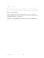
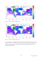
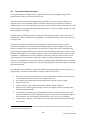
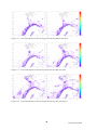
Select a large set of data, for example one month.
Computationally limit the field of view to an along track oriented box with all sides
equal to 60% of the full field of view. The purpose of this box is to ensure that repeat
passes have similar geometries.
Compute when each cell is visible within the satellite’s boxed field of view.
Extract consecutive passes for each cell, i.e. the time between the first pass and second
pass must be equal to the period of the orbit.
For each pair of passes for each cell: Extract all messages received within the first and
second pass. The first pass is used to identify the vessels within each cell. The second
pass is used to compute the detection probability by simply identifying the fraction of
vessels seen in the second pass out of those seen the first. This algorithm does not require
that the vessels detected in the second pass are still within the cell. Some vessels may
have moved outside the cell since the first pass.
Each cell then gets assigned the average number of detected vessels per pass and an
average detection probability. The vessel model is created by sampling from these cells
using observed positions to avoid 1x1 degree blocks in the final distribution. This step is
done for each possible repetition rate.
There are some problems with this algorithm: Vessels may change repetition rates between and
even during passes. Vessels that transmit with too low power to be detected will not be included
in the model. There are areas where the detection probability is too low to give any meaningful
statistics. These areas must be excluded from the model, and are shown as green, blue and cyan in
Figure 2.1. Finally, vessels that transmit once every third minute are difficult to detect, and the
observations do not give sufficient data to derive a traffic model. The number of vessels that
transmit every third minute was therefore scaled to ensure similar numbers as seen in areas with
known distributions.
2.2
Detection probabilities and vessel distribution maps
Figure 2.1 shows the detection probabilities derived using the algorithm described in section 2.1.
This figure is based on AIS data received by the International Space Station (ISS) during March
2011. March 2011 was selected because there was very little interference from other equipment
on the ISS. Communication on one of S-band antennas on the station tends to interfere with the
AIS receiver. The effect of this interference can be seen by comparing Figure 2.1 and Figure 2.2,
which is based on data recorded in August 2011.
Appendix A.1 shows the commands that created the vessel density maps shown in this section.
8
FFI-rapport 2012/00048