1
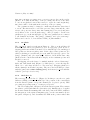
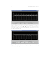
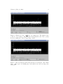
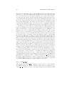
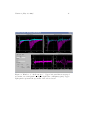
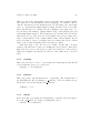
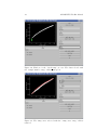
Version 1 (May 13, 2008)
1
AKARI FTS Toolkit Manual
Version 1
Hidenori Takahashi1 , Yoko Okada2 , Akiko Yasuda2 ,
Hiroshi Matsuo3 , Mitsunobu Kawada4 , Noriko
Murakami5 , and Chris Pearson6,7
1 Gunma
Astronomical Observatory
of Space and Astronautical Science (ISAS), JAXA
3 National Astronomical Observatory of Japan
4 Nagoya University
5 Bisei Astronomical Observatory
6 CCLRC Rutherford Appleton Laboratory
7 University of Lethbridge
2 Institute
May 13, 2008
Version 1 (May 13, 2008)
Date
5 December 2007
6 December 2007
29 December 2007
7 January 2008
14 January 2008
23 April 2008
12 May 2008
i
Revision
Version 0.9
Version 0.91
Version 0.92
Version 0.93
Version 0.94
Version 0.95
Version 1
Comments
First Draft Hidenori Takahashi
Updated Format Chris Pearson
Updated Yoko Okada
Updated Chris Pearson
Updated Yoko Okada
Updated Yoko Okada
Updated Yoko Okada
ii
AKARI FTS Toolkit Manual
Contents
1 Data Preparation
2 fts part1
2.1 Details of GUI processes
2.1.1 check ramp curve
2.1.2 check reset bad .
2.1.3 rm glitch . . . .
2.1.4 check drv cb . .
2.1.5 check all cb . . .
2.1.6 check raw spec .
2.2 options for fts part1 . .
2.2.1 plotch . . . . . .
2.2.2 rampcorr . . . .
2.2.3 rampbflg . . . .
2.2.4 addname . . . .
2.2.5 vifbadf . . . . . .
2.2.6 mcal . . . . . . .
2.2.7 pixflg . . . . . .
2.2.8 sigmaclip . . . .
2.2.9 setcbp . . . . . .
2.3 Contents of the save file
2
. . .
corr
. . .
. . .
. . .
. . .
. . .
. . .
. . .
. . .
. . .
. . .
. . .
. . .
. . .
. . .
. . .
. . .
.
.
.
.
.
.
.
.
.
.
.
.
.
.
.
.
.
.
.
.
.
.
.
.
.
.
.
.
.
.
.
.
.
.
.
.
.
.
.
.
.
.
.
.
.
.
.
.
.
.
.
.
.
.
.
.
.
.
.
.
.
.
.
.
.
.
.
.
.
.
.
.
.
.
.
.
.
.
.
.
.
.
.
.
.
.
.
.
.
.
.
.
.
.
.
.
.
.
.
.
.
.
.
.
.
.
.
.
.
.
.
.
.
.
.
.
.
.
.
.
.
.
.
.
.
.
.
.
.
.
.
.
.
.
.
.
.
.
.
.
.
.
.
.
.
.
.
.
.
.
.
.
.
.
.
.
.
.
.
.
.
.
.
.
.
.
.
.
.
.
.
.
.
.
.
.
.
.
.
.
.
.
.
.
.
.
.
.
.
.
.
.
.
.
.
.
.
.
.
.
.
.
.
.
.
.
.
.
.
.
.
.
.
.
.
.
.
.
.
.
.
.
.
.
.
.
.
.
.
.
.
.
.
.
.
.
.
.
.
.
.
.
.
.
.
.
.
.
.
.
.
.
.
.
.
.
.
.
.
.
.
.
.
.
.
.
.
.
.
.
.
.
.
.
.
.
.
.
.
.
.
.
.
.
.
.
.
.
.
.
.
.
.
.
.
.
.
.
.
.
.
.
.
.
.
.
.
.
.
.
.
.
.
.
.
.
.
.
.
.
.
.
.
.
3
5
5
6
7
7
10
13
13
16
16
17
17
17
20
20
20
20
20
3 FTS tools
23
3.1 fts checkrawspec . . . . . . . . . . . . . . . . . . . . . . . . . 23
3.2 fts part1 output . . . . . . . . . . . . . . . . . . . . . . . . . 23
Version 1 (May 13, 2008)
1
About this Document
This document explains how to analyze AKARI Fourier Transform Spectrometer (FTS) data. The analysis procedure consists of two main steps.
The first processing step, f ts part1, carries out the Fourier transformation
of the interferogram obtained from the time series data (TSD) to provide
the spectral information. The second processing step carries out the flux
and wavelength calibrations on each channel. Since the latter calibration
part is still under development, only the former part, f ts part1 is described
in this document. Calibration part will be released in a later version.
All procedures are based on the IDL programming language. In this
document, it is assumed that the FIS IDL procedures and IDL itself are
already installed and running in your environment. More information on
the basics of the AKARI data flow, FIS analysis tools, and strategy for
data processing using the FTS can be found in the FIS Instrument Data
User Manual (IDUM). The definition of the FIS channel numbering follow
Figures 2.1.6 or 3.2.9 in the FIS IDUM.
In the following sections, processing with many iterative steps will be
described:
1. Data preparation,
2. fts part1,
3. FTS tools
Definition of words
GB
OPD
TSD
ZPD
Green Box
optical path difference
time series data
zero path difference
centerburst
The standard FIS pipeline tool.
The format of the raw data.
The position where the optical path difference
is zero.
Same as ZPD, though also used for the whole
structure in interferogram around ZPD.
2
1
AKARI FTS Toolkit Manual
Data Preparation
Suppose the file name of the raw observations data set (TSD) as input base+“fits.gz”.
Before running the f ts part1 processing step, it is required to separate the
target observation data from the calibration data, etc., in the raw data set.
The task is performed by the following simple IDL command:
FISDR> fts mk obj mcal acal,input base+‘fits.gz’ [,/noobj] [,/nomcal]
[,/noacal] [,/nodark]
Just type f ts mk obj mcal acal to display the usage. f ts mk obj mcal acal
makes several subsets from the TSD fits file of one pointed observation.
Output files have extra characters between input base and ‘fits.gz’, which
represent the contents of the subset. “obj” means the celestial object data,
“mcal” means the internal calibration light source data, “dark” means dark
data, and “acal” means the cal-A lamp data. “dark1”, “dark2”, and “dark3”
refer to the dark data before the observation, between the observation of the
internal calibration lamp and the celestial object, and after the observation,
respectively. “acal b” and “acal a” are the cal-A lamp data before and after
the observation, respectively. If only selected subsets are required, options
can be set to omit the unneeded subsets, e.g. setting the /nomcal option
will omit the “mcal” data subset.
Either of input base+‘obj.fits.gz’ or input base+‘mcal.fits.gz’ becomes
the input for the f ts part1 procedure.
Version 1 (May 13, 2008)
2
3
fts part1
The f ts part1 process carries out the Fourier transformation of the time
series data (TSD) to obtain spectral information. The processing steps are
given below. During the processing, there will be several GUIs for checking
of data, flagging and corrections. Additional optional parameters used at
the startup of f ts part1 are summarized in section 2.2
[Raw data]
1. ADU to voltage conversion (GB pipeline tool)
2. Ramp curve correction (GB pipeline tool with correction table optimized for FTS observations)
Correct for non-linearity of the ramp curve.
GUI : check ramp curve corr
• Quality check of the ramp curve correction.
3. Differentiation (GB pipeline tool)
[Interferogram + DC component]
4. Separate into individual scans
5. Remove reset anomaly
GUI : check reset bad
• Removal of any data affected by resets.
6. Remove glitches
GUI : rm glitch
• Masking glitches by eye if necessary.
7. Subtract DC component
4
AKARI FTS Toolkit Manual
8. Interpolation of bad data
Replace any bad data by the median of other scans. Since the first scan
in SED mode is affected by an irregular drive pattern at the starting
point, we ignore the first scan when calculating the median in the SED
mode.
9. Determine the zero path difference (ZPD) in a specific channel
Since the value of the position sensor is correct only relatively, the
ZPD must be determined. The present toolkit determines the ZPD
that minimizes the squared imaginary part integrated over the effective
wavenumber.
GUI : check drv cb
• Check the estimated ZPD for the every scan in a specific channel
and tune parameters to reject incorrect estimates.
10. Determine the ZPD in all channels
It is assumed that the relative deviation of the ZPD between different
scans is the same for all channels. And the ZPD of all the channels
are estimated in this step.
GUI : check all cb
• Check the estimated ZPD for all channels and tune parameters
to reject incorrect estimates.
11. Discrete Fourier Transform
Apply Discrete Fourier Transform using the output of the position sensor and the determined ZPD in the previous steps to the interferogram
of each and every scan.
12. Average the spectra
After applying Fourier transforms, the average spectrum is taken.
GUI : check raw spec
• Check the Fourier transformed spectra for all channels.
[Raw spectra] (final output of the f ts part1)
Version 1 (May 13, 2008)
5
To start the process, from IDL command line, input the following command
FISDR> fts part1, input base+‘obj.fits.gz’ [,plotch = integer]
[,rampcorr = 1,2,3 or string] [,/mcal] [,/sigmaclip]
Just type fts part1 to display the usage. Refer to Section 2.2 for a detailed
description of the available options. The rampcorr option (see 2.2.2) is used
to select the appropriate ramp curve correction table. It is not necessary
to specify rampcorr except for very bright objects, and in most cases the
default correction table is used. The plotch option (see 2.2.1) is used to select
a specific channel used for the adjustment of the ZPD. For observations of
point or small extended sources it is necessary to set the channel in which the
source is detected as plotch. For large extended sources, it is not necessary
to specify plotch, and the default channels (channel 23 for SW and 7 for
LW) will be used. The mcal option (see 2.2.6) should be used when the user
process the data of the internal calibration lamp. The sigmaclip option (see
2.2.8) is for automatic glitch removal. We recommend to use this option,
otherwise the user will have to remove all glitches manually by eye. The
following sub-section describes the details of GUI processes.
2.1
2.1.1
Details of GUI processes
check ramp curve corr
The standard FIS pipeline tool (Green Box) is used to correct for any nonlinearity of the ramp curves (see FIS Instrument Data Users Manual Section
4.1.2). The correction table optimized for FTS observations has been prepared in the toolkit and used for nominal FTS observations. For very bright
targets whose brightness exceeds the range of the correction table, a correction table should be made from the data itself, setting rampcorr=1. In this
case, see Section 2.2.2 for detailed explanations of this option.
This process opens a window ‘check ramp curve corr’ as shown in Figure 1 which has three panels; the lower left panel shows the raw integrated
time series data, the lower right panel shows the relation of the ramp curve
correction (white: measured, red: corrected), and the upper panel displays
the derivative of the raw data and ramp curve corrected data of the selected
channel. One should check on the upper panel whether the corrected interferogram (blue) is flat, except for the centerburst, compared to the original
6
AKARI FTS Toolkit Manual
data (white). In general the correction is smaller for the LW band than the
SW band. The display range can be changed by using the [range] button.
When it is acceptable, click [ok] to progress to the next step. If something
is unsatisfactory or wrong you may have to quit and start again using a
different option.
Figure 1: Window for the ”check ramp curve corr” process. The white and
blue lines in the upper panel represent the interferograms before and after
correction respectively.
2.1.2
check reset bad
This step removes reset anomalies. During this step, the ‘check reset bad’
window can be viewed, as shown in Figure 2.
Using this GUI, user should examine the data to ensure that the reset
periods are properly flagged out. Flagged data itself have the value ‘-999’
and reach far below the window. If the flag is not properly set, there will be
periodic glitches before or after the reset as shown in Figure 2. Normally,
the reset anomalies can be flagged using the default parameters. If periodic
glitches as exemplified in Figure 2 are found, check the ramp curve correction
Version 1 (May 13, 2008)
7
first, since an improper ramp curve correction can produce such periodic
glitches. Note that at this stage of the processing, the user does not have
to care about glitches between the resets (i.e. aperiodic, random glitches),
since these will be dealt with in the next step of the processing.
Two parameters may be changed to mask any anomalous data related
to resets. The first is used to select the pre-reset data points and the other
refers to the post-reset data points. After tuning the [before reset] and [after
reset] sliders of the “reset anomaly range”, click [do again] to set the new
parameters (e.g. as shown in Figure 3). The reset parameters are common
to all channels and scans. The [range], [channel], and “plot scan range”
sliders can be used to look at all data. Click [ok] when finished.
2.1.3
rm glitch
The ‘rm glitch’ window is shown in Figure 4. Here you should flag all
individual data affected by glitches by eyes. If sigmaclip option is set, σclipping glitch removal has been made before this GUI process, and flagged
data points are shown as pink points. If the clipped data points are not
valid, break this process and run f ts part1 without sigmaclip option. Use
[range], [channel], and “plot scan range” sliders to check all the data. Any
glitch near the centerburst will affect largely on the resultant spectra and
should be removed.
For flagging, select the data to be masked with the “selected data range”
slider and click [mask data] (Figure 5). Click [save] to create the flag file.
Click ‘ok’ to save flags and move to the next step. Flagging glitches for
all the channels often takes long time. The user can break this procedure
with the [quit] button after clicking [save], and restart f ts part1 with the
‘vifbadf’ option (see Section 2.2).
2.1.4
check drv cb
The next step is “check drv cb” (Figure 6). In this process, the zero path
difference (ZPD) position is identified (i.e. the position of the centerburst)
from the interferograms of a specific channel (set by plotch option). This
processing step is important to obtain proper spectra.
The lower right panel of Figure 6 shows the interferogram. The x-axis is
the relative optical path difference (hereafter opd). Initially, the tool applies
the Fourier transform assuming that each data point is the ZPD, estimates
the integration of the squared imaginary part over the wavenumber (lower
left panel of Figure 6), and determines the ZPD as the position where this
8
AKARI FTS Toolkit Manual
Figure 2: Window for the ”check reset bad” processing step. Note that the
data just before reset overshoots above the mean level of the interferogram.
The value of flagged data is -999, and apparent overshoots the bottom of
the window represent -999.
Figure 3: The overshot data seen in the previous figure are removed using
the reset anomaly range.
Version 1 (May 13, 2008)
9
Figure 4: Window for the ”rm glitch” processing step. The glitch at the
position corresponding to sample number 1841 (shown by the ”blue” point)
is selected using the ”selected data range” slider.
Figure 5: After selecting the glitch data as in the previous figure, click “mask
data”. After replot by clicking any of the sliders, the removed data point
turns pink.
10
AKARI FTS Toolkit Manual
integration is a minimum. The determined ZPD is shown as a white (forward
scan case) or yellow (backward scan case)line in the lower right panel and
the red point in the lower left panel. Using the “zero-path position” slider,
you can select the data point and check the interferogram (blue line in the
lower right panel), the integration of the squared imaginary part (blue point
in the lower left panel) and the spectra itself under the assumption that
this point is ZPD (upper left panel; red represents the real part and blue
represents the imaginary part). You can select the scan number using the
“scan” slider. The upper right panel shows the derived ZPD for each scan.
At this stage, it is necessary to check whether the ZPDs in all the scans
have been estimated correctly. Though the definition of the ZPD is the opd
where the integration of the squared imaginary part is a minimum, local
minima next to the real ZPD may have smaller values in the case of data
with low S/N or data affected by strong transient effects. There are two
check points that can prove useful. The first is whether the interferogram
is a positive peak or a negative peak at the ZPD (see white or yellow lines
in the lower right panel of Figure 6). For celestial data taken in the SW
band and internal calibration data with LW, the interferogram should exhibit a negative peak at the ZPD. For celestial data taken in the LW band
and internal calibration data with SW, the interferogram should exhibit a
positive peak at the ZPD. The second check point regards the upper right
panel. Since the ZPD does not change significantly between scans, the upper
right panel should appear almost constant (except for the first scan). If you
discover any large discrepancy (over 0.002 cm) between scans as exemplified
in Figure 6, the determined ZPDs in some scans are probably not correct.
If the determined ZPDs are acceptable, click [ok] to finish this procedure.
If not, tune the ZPD using four sliders at the bottom of the window, which
cover the range of the opd used to determine the ZPD. For example in
Figure 6, improper positions of opd > −0.002 cm are selected as the ZPD in
several backward scans (see upper right panel). Moving the lower right slider
(maximum for backward scan) to −0.002 and clicking [do again], produces
the window shown in Figure 7 (after a short wait). Note that the newly
determined ZPDs seem to be correct for all the scans. This process should
be repeated until the ZPDs for all the scans are acceptable.
2.1.5
check all cb
The next step is ”check all cb” (Figure 8) and is used to check whether
the ZPD is reliable for all the channels. The window is similar to the
“check drv cb” window, except for the upper right panel, in which the ZPD
Version 1 (May 13, 2008)
11
Figure 6: Window of ”check drive cb” in the case of LW channel 7 of a
celestial object. The red point in the lower left panel shows the selected
opd, where the integration of the square of the imaginary part is a minimum.
However, this is in the negative peak of interferogram as shown in the lower
right panel, whereas the interferogram of celestial objects observed in the
LW band should be the positive peak at ZPD. It can also be found that the
relative optical path difference of this scan (= 3) is not in agreement with
that of the majority of other scans in the upper right panel.
12
AKARI FTS Toolkit Manual
Figure 7: After tuning the slider, the ZPDs in all the scans are determined
correctly.
Version 1 (May 13, 2008)
13
for every scan is replaced by that of the channels (Figure 8). The procedure
of this tool is similar to that of “check drv cb”. Since there is no need to
select forward or backward scans, only two sliders are available, instead of
four. Note that the ZPD of bad channels any channels in which objects are
not detected is not trustworthy and may be ignored.
2.1.6
check raw spec
After applying Fourier transforms to the interferogram of each and every
scan, the average spectrum is taken. As final products, spectra of complex
type are obtained. The real part corresponds to spectra with physical meaning, and the imaginary part is residual of the phase correction. Note that
the imaginary part of the full-resolution mode data does not represent this
residual correctly, since the Fourier transform is applied only for one-side of
the centerburst.
This step is primarily for confirmation (Figure 9). The upper left and
upper right panels show the averaged spectrum and the spectrum of selected
scans, respectively. The plot can be adjusted by using several available
buttons. Use the ”quit” button to finish f ts part1 processing.
2.2
options for fts part1
In this section, we explain the optional commands which are available to the
user in the f ts part1 processing step of the toolkit.
option
plotch = integer
rampcorr = 1,2,3 or string
rampbflg = string
addname = string
vifbadf = string
/mcal
pixflg = integer vector
/sigmaclip
/setcbp
explanation
channel for the adjustment of the ZPD of each scan
select ramp curve correction table
use previously saved ramp flag file
add optional characters to output files
use previously saved glitch flag file
required to process internal calibration source data
flag all data on specific channels
flag bad data by σ-clipping before “rm glitch” GUI
establish ZPD from driving pattern automatically
14
AKARI FTS Toolkit Manual
Figure 8: Window for the ”check all cb” processing step. This window is
similar to that of ”check drv cb” except the upper right panel represents
every channel rather than every scan. Note that there is a trend to incline
on each row in the case that a large extended object is detected over several
channels.
Version 1 (May 13, 2008)
15
Figure 9: Window of ”check raw spec”. Upper left panel shows averaged
spectrum over scans (pink = real part, light blue = imaginary part). Upper
right panel represents the spectrum of the selected scan.
16
2.2.1
AKARI FTS Toolkit Manual
plotch
The plotch option is used to select a specific channel for the adjustment
of the ZPD of every scan, used in “check drv cb”. A channel which detects sufficient photons with high S/N is recommended. For large extended
sources the default channels (channel 23 for SW and channel 7 for LW) are
recommended, so it is not necessary to set this option. For point or small
extended sources, a channel in which the sources are detected should be
set: plotch = 28 or 29 and plotch = 4 or 5 for SW and LW observations,
respectively, with AOT parameters of FIS03;*;*;1, plotch = 54 or 55 and
plotch = 23 for SW and LW observations, respectively, with AOT parameters of FIS03;*;*;2, and plotch = 32 or 33 (or 53) and plotch = 7 for SW
and LW observations, respectively, with AOT parameters of FIS03;*;*;0.
2.2.2
rampcorr
The ramp curve correction table is selected by rampcorr option. By default,
the correction table in the toolkit for FTS observations, which is recommended for most data, is used. This option accepts either an integer 1, 2, 3
or a string of a ccf filename.
1 : Make a correction table using the data itself. This is required for very
bright objects.
2 : Apply correction table for survey mode data. Not recommended (test
purpose).
3 : No correction. Not recommended (test purpose).
ccf file name (string) : select specific ramp curve correction table. See below.
Processing with rampcorr=1, generates a ramp curve correction table
file named “***ramptbl.ccf”. Once a correction table is made for one observation, the user can use it every time by specifying the file as rampcorr=“***ramptbl.ccf ” instead of making the correction table again.
If rampcorr = 1 is selected, the ”check ramp” monitor window appears
(Figure 10). All ramp curves (far from the centerburst) used to make a
correction table are plotted in the top-left window. Unsuitable ramp curve
data should be flagged in this step. A channel is selected using the [channel]
slider. There are two additional sets of sliders, ”ramp curve range” and
”sample number range”. The former is used to remove a ramp curve, and
the latter is used to remove data of the same sample number from all ramps.
Version 1 (May 13, 2008)
17
When you select the “all channel” button, the same data points are simultaneously removed in all channels, whereas using the “one channel” button,
only the data in the selected channel is removed. The first point of the ramp
curve, i.e. data with the sample number being 0, should be removed because
these data should not be included as the beginning of the ramp curve. Select the first point with the “sample number range” slider (Figure 10), and
click [mask sample number]. The actual removal of a ramp curve follows the
same methodology of the removal of bad sample data except “ramp curve
range” is used instead of the “sample number range” sliders (Figure 11). It
is not necessary to remove bad ramp curves very finely, since most of them
will be removed automatically in the following processing.
Click [save flag] to save the above processing. At any time, one may
return to the last saved position by clicking the [reset] button. Click [save
flag] and [ok] to move to the next procedure, the derivation of the averaged
ramp curve (Figure 12) and the production of the ramp curve correction
table.
2.2.3
rampbflg
This option is used to refer to a previously saved ramp flag file and should
be used with the rampcorr=1 option set.
rampbfig = ‘*****ramp.sav’
2.2.4
addname
This option adds optional characters to output files. The default name of
the final IDL save file is ”filename + part1.sav”. The new characters are
inserted in between the filename and part1.sav.
addname = ‘****’
2.2.5
vifbadf
If the users have previously saved flagging file of glitches, the users import
it for the ”rm glitch” processing by setting this option.
vifbadf = ‘*****vifbad.sav’
18
AKARI FTS Toolkit Manual
Figure 10: Window for the ”check ramp” process. The data selected with
the “sample number range” sliders turn green.
Figure 11: The ramp curve selected with the “ramp curve range” sliders
turn red.
Version 1 (May 13, 2008)
19
Figure 12: Window to check the averaged ramp curve. White lines are all
the ramps with scaling and the blue line is the assumed average. Click [ok]
to continue.
20
AKARI FTS Toolkit Manual
2.2.6
mcal
This option should be used when processing the data of the internal calibration light source. The temperature of the internal calibration source
becomes stable only after several scans, thus the data of first 3 scans and
last scan is discarded with this option.
/mcal
2.2.7
pixflg
This option is used to flag all data on specific channels, e.g. saturated
channels, in addition to LW[2,3,18,33,42] and SW[1,11] which are already
known to be bad channel.
pixflg = [6,7,31]
2.2.8
sigmaclip
Flag bad data by σ-clipping before glitch-check GUI.
/sigmaclip
2.2.9
setcbp
The ZPD is automatically established from the driving pattern with this
option. This option should be used only for faint sources which do not have
a clear centerburst and for which the ZPD can not be determined from the
data itself.
/setcbp
2.3
Contents of the save file
During the f ts part1 processing, several ”save files” are created. Note that
the creation of some files depend on the options employed.
Version 1 (May 13, 2008)
21
*** part1.sav : final output of fts part1
*** vifbad.sav : bad flag data of glitches created in ”rm glitch”
***ramp.sav : bad flag data of ramps created by [save] button in ”check ramp”
(with option rampcorr=1)
***.ramptbl.ccf : ramp curve correction table (with option rampcorr=1)
***ramp*.ps : Some postscript files produced during the process of making
the ramp curve correction table (with option rampcorr=1)
Major contents of *** part1.sav
• VER (STRING) : Version of fts part1
• FILENAME0 (STRING) : The name of the input TSD file
• DATATYPE (STRING) : ‘FIS SW’ / ‘FIS LW’
• PKTID F (BYTE) : 124 (for SED mode) / 14 (for Full-resolution
mode)
• RSEXT (INT = Array[2]) : Removed reset point [pre, post]
• PCH (INT) : = plotch-1
• RADEC A (DOUBLE = Array[2, ndet all]) : Equatorial coordinate of
each channel calculated from AOCU. RADEC A[0, *] is RA, RADEC A[1,
*] is DEC in degree. See FIS IDUM for attitude determination.
• RADEC G : Same as RADEC A but calculated from G-ADS.
• VIFBAD (INT = Array[ndata, ndrv, ndet]) : Flag of the interferogram
• RANGE (DOUBLE = Array[2]) : Range of data for Fourier transform
[cm]
• DC (DOUBLE = Array[ndrv, ndet]) : Non-interferometric component,
which is an averaged interferogram over a scan.
• VIF (DOUBLE = Array[ndata, ndrv, ndet]) : Interferogram of each
scan and channel
• VIFPOS (ODUBLE = Array[ndata, ndrv]) : Optical path difference
in each scan for PCH ([cm])
• WN (FLOAT = Array[nwn]) : Wavenumber [cm−1 ]
22
AKARI FTS Toolkit Manual
• SPEC (DOUBLE = Array[nwn, 2(average/stdv), 3(real/imaginary/phase),
2(forward/backward),ndet]) : Averaged spectrum
• SPECBARA (DOUBLE = Array[ndrv, nwn, 3(real/imaginary/phase),
2(forward/backward), ndet]) : Spectrum of each scan
ndet = Number of channels for WIDE band (SW/LW = 60/45)
ndet all = Number of channels for WIDE and NARROW band (SW/LW
= 100/75)
ndrv = Number of scans
ndata = Number of data per scan. For SED mode observations, the first
half of the data corresponds to the forward scan and the last half to
the backward scan. For Full-resolution mode, the first half of the data
corresponds to the backward scan and last half corresponds to the
forward scan.
nwn = Number of wavenumber elements in the spectrum
Version 1 (May 13, 2008)
3
23
FTS tools
Two tools are provided to support the FTS data reduction. Typing without
argument will display the usage. Suppose the file name of the final output
of fts part1 as input base+‘part1.sav’ in the following.
3.1
fts checkrawspec
The “check raw spec” window (Figure 9) is opened by this command. plotch
specifies the channel to plot, though this can be changed using the GUI.
FISDR> fts checkrawspec,filename=input base+‘part1.sav’[,plotch=*]
3.2
fts part1 output
This procedure makes postscript or ascii files from input base+‘part1.sav’.
FISDR> fts part1 output, input base+‘part1.sav’ [,/mcal] [,addname =
string] [,/psfile] [,fixmin = value] [,fixmax = value] [,wnmin = value] [,wnmax
= value] [,/txtfile] [,txtch = integer vector]
If the user wants to obtain a postscript file to show the raw spectra of
all the channels, set psfile option. Then input base+‘part1.ps’ file is created.
The minimum or maximum values of x- and y-axis can be specified for all
the channels by the options wnmin, wnmax, fixmin and fixmax, respectively.
If the user wants to obtain an ascii file of the raw spectra, set txtfile
option, then input base+‘part1.txt’ file is created. By default, the data of
all the channels are included. Data of specific channels can be extracted by
txtch option, e.g. txtch = [33,34,35].
/mcal option should be given when the user processes the data of the
internal calibration lamp. The addname option can be used to add a word
between ‘part1’ and ‘.ps’ or ‘.txt’ of output files.