1
OCCAM: A Reconstructability Analysis Program
(Organizational Complexity Computation and Modeling)
Joe Fusion, Kenneth Willett and Martin Zwick
Systems Science Ph.D. Program; Portland State University, Portland OR 97207
This manual was last revised on: 11 May 2012.
Occam version 3.3.4, copyright 2006-2012.
Table of Contents
I. For Information On Reconstructability Analysis
2 II. Accessing Occam
2 III. Search Input
3 IV. Search Output
13 V. State-Based Search
15 VI. Fit Input
16 VII. Fit Output
17 VIII. State-Based Fit
18 IX. Show Log
18 X. Manage Jobs
18 XI. Frequently Asked Questions
18 XII. Error And Warning Messages
23 XIII. Known Bugs & Infelicities; Limitations
24 XIV. Planned But Not-Yet-Implemented Features
25 Appendix 1. Rebinning (Recoding)
27 Appendix 2. Missing Values In The Data
29 Appendix 3. Additional Parameters In The Input File
29 Appendix 4. Zipping The Input File
30 Occam User’s Manual
5/12/2012
2
I. For Information On Reconstructability Analysis
For papers on Reconstructability Analysis, see the Discrete Multivariate Modeling page
at http://www.pdx.edu/sysc/research-discrete-multivariate-modeling. For an overview of
RA, see the following two papers that are on the DMM page:
“Wholes and Parts in General Systems Methodology” at
http://www.sysc.pdx.edu/download/papers/wholesg.pdf
“An Overview of Reconstructability Analysis” at
http://www.sysc.pdx.edu/download/papers/ldlpitf.pdf
II. Accessing Occam
Occam location & general use
Occam3 is at: http://dmm.sysc.pdx.edu/. It can also be accessed from the DMM web
page: http://www.pdx.edu/sysc/research-discrete-multivariate-modeling.
Occam runs on a PSU server. The user uploads a data file to this server, provides
additional input information on a web input page, and then initiates Occam action. When
the computation is complete, Occam either returns HTML output directly to the user, or a
.csv output file that can be read by a spreadsheet program such as Excel. If the
computation is not likely to finish rapidly, the user can provide an email address and
Occam will email the output (in .csv form) when it is done.
Notify us of program bugs & manual obscurities/errors
If you encounter any bugs or mysterious output, please check to see that your input file
matches the format requirements specified below. If you are confident that your input file
is formatted correctly, email it to us at: [email protected]. Please include
the settings used on the web page, a description of the problem, and the Occam output if
available. (If your input file is large, please zip it before attaching to your email.)
We also need your support in maintaining this user’s manual. Please let us know if there
is information missing in this manual that you need, if explanations are obscure, or if
there are any errors. Email your comments to: [email protected].
Action
When one brings Occam up, one first must choose between several Occam actions. The
modeling options are: “Do Fit,” “Do Search,” “Do SB-Fit,” and “Do SB-Search.” There
are also options for “Show Log” and “Manage Jobs,” which allow the user to track the
status of jobs submitted for background processing. You can see this first web page by
clicking on: http://dmm.sysc.pdx.edu/weboccam.cgi.
When an option is selected, Occam returns a window specific to the choice made. Search
assesses many models either from the full set of all possible models or from various
partial subsets of models. Fit examines one model in greater detail. In an exploratory
mode, one would do Search first, and then Fit, but in a confirmatory mode, one would
Occam User’s Manual
5/12/2012
3
simply do Fit. The options for SB-Fit and SB-Search function similarly, but for statebased models, rather than the default variable-based models. Let’s focus first on the main
option of “Do Search.”
III. Search Input
On the first line, the user must specify a data file, which not only provides the data to be
analyzed but also describes the variables used and allows the user to set certain
parameters. After the data file will now be discussed, the other parameters on this input
page will be explained.
Data file
The user must specify a data file on the user’s computer by typing its name (and location)
in or finding it by browsing. The data file is then uploaded to the Occam server. This is
actually all that is needed to submit an Occam job, if the user is satisfied with the default
setting of all the parameters.
Data files should be plain-text ASCII files, such as those generated by Notepad, or Word
or Excel if the file is saved in a .txt format. (Note that in Excel, you should not use the
“Space Delimited Text” format, with the .prn extension, as it can be incompatible with
Occam.) Each line of the data file has a maximum length, currently set to 1000
characters. Occam will give an error if this is exceeded. If your data set requires lines
longer than this limit, please contact the feedback address listed above.
A minimal data file looks like this. (This is the data from the “Wholes & Parts” paper.)
:nominal
alpha,
beta,
gamma,
:data
0
0
0
0
1
1
1
1
0
0
1
1
0
0
1
1
2,1,a
2,1,b
2,2,c
0
1
0
1
0
1
0
1
143
253
77
182
227
411
46
139
This simple file has 2 parts: (1) specification of the variables, and (2) the data to be
analyzed. Each part in this example begins with a line of the form “:parameter”, where
“parameter” is “nominal”, or “data”.
Variable specification
Variable specification begins with “:nominal” which reminds the user that nominal
(categorical, qualitative) variables must be used. (For tips on binning quantitative
variables, see FAQ #6.) After “:nominal”, the variables are specified, one per line,
ignoring white space between values. In the above example, the first line is:
Occam User’s Manual
5/12/2012
4
alpha, 2,1,a
“alpha” is the name of the first variable. The second field indicates that it has 2 possible
states (a “cardinality” of 2). The third field (shown above as 1) is 0, 1 or 2. A value of 1
defines the variable as an “independent variable” (IV) or input. A value of 2 defines it as
a “dependent variable” (DV) or output. A value of 0 means that the variable (and the
corresponding column in the data) will be ignored. This allows the user to have data for
more variables than can be analyzed at any one time; the user could then easily alter
which variables are to be included in the analysis and which are to be omitted. The value
of 0 in the third field also supersedes any rebinning specification (described below); the
rebinning string will be completely ignored if the third field is 0. If all variables are
designated as IVs (1) or as DVs (2), the system is “neutral.” If some variables are IVs,
and at least one is a DV, the system is “directed.” The above data file is for a directed
system.
The fourth field is a variable abbreviation, usually one letter. Lower case letters may be
used, but will appear in Occam output with the first letter capitalized. In the above
example, variable “alpha” will be referred to in Occam output as “A”. If there are more
than 26 variables, one can use double (or triple, etc.) letters as abbreviations, for example
“aa” or “ab”. (Such variables would appear in model names as AaB:AbC, for example.)
Variable abbreviations must be only letters; numbers or other symbols may not be used to
abbreviate variables. (Numbers are reserved for use as state names, particularly in StateBased RA, where variable abbreviations and state names must not overlap.)
Although data submitted to Occam must already have been binned (discretized), an
optional fifth field tells Occam to “rebin” the data. Rebinning allows one to recode the
bins by selecting only certain bin values for consideration or for omission, or by
aggregating two or more bins. This is discussed in depth in Appendix-1.
Data specification
The second part of this file is the data, which follows the “:data” line. In the data,
variables are columns, separated by one or more spaces or tabs. The columns from left to
right correspond to the sequence of variables specified above, i.e., the first column is
alpha, the second beta, and the third gamma. Following the variable columns there can be
an additional column that gives the frequency of occurrence of the particular state
specified by the variable values. The frequency value does not have to be integer, so
frequencies that become non-integer because some weighting has been applied to them
are okay. However, frequency values may not be negative.
Note that since non-integer frequencies are allowed, one can use Occam to analyze–and
compress–arbitrary functions of nominal variables. Occam simply scales the function
value so that it can be treated as a probability value, and then does a decomposition
analysis on this “probability distribution.” In the RA work of Bush Jones, this is called
“g-to-k” normalization. Note, however, that if Occam is used in this way, statistical
measures like alpha that depend on sample size do not have their usual interpretation.
Occam User’s Manual
5/12/2012
5
Since variables are nominal, their values (states) are names. Normally, these will be
0,1,2… or 1,2,3… but the character “.” is also allowed, e.g., to designate missing values.
(Note that when using “.” it must be included in the cardinality of the variable.) No other
non-numeric characters are allowed as variable states. To avoid possible confusion, it is
best to start the labeling of all variables either with 0 or with 1, i.e., avoid starting one
variable with 0 and another with 1 (though Occam can handle such inconsistencies of
convention). The user should know the number of different states that occur for each
variable and indicate the cardinality of the variable correctly in the variable specification.
Data can be provided to Occam without frequencies, where each line (row) represents a
single case. The rows do not have to be ordered in any particular way. Occam will
generate the frequencies itself, but it needs to be told that the data do not include
frequencies, as follows:
:no-frequency
:data
0
1
0
1
0
0
0
0
1
1
1
1
0
1
1
0
0
1
1
0
0
0
1
1
0
1
1
1
1
0
1
1
0
1
0
1
Uploading data will be faster if the data provides frequencies, so if the data file is big, the
user might consider doing this operation before calling Occam.
Test data specification
Optionally, a data file can include “test data.” Typically, test data are a fraction of the
original data that has been set aside, so that models can be measured against data that
were not used in their creation. In Search, if test data are present and the “Percent
Correct” option is checked, the report will include the performance of the models on the
test data. In Fit, the performance of the model on test data is show automatically,
whenever test data are present. To include test data in a data file, use the “:test”
parameter, followed by lines of data in the same format used for “:data”.
:test
0
0
0
0
1
1
1
1
0
0
1
1
0
0
1
1
0
1
0
1
0
1
0
1
70
125
26
100
120
190
25
80
Occam User’s Manual
5/12/2012
6
Comments in the data file
A line beginning with “#” will be ignored when Occam reads the data file, so this
character can be used to begin comment lines. Also on any given line, Occam will not
read past a “#” character, so comments can be added at the end of lines which provide
actual input to the program. Comments do not count toward the maximum line length
mentioned above.
Web input
We now discuss the other parts of the Search web input page.
General settings
Starting Model
Occam searches from a starting model. This can be specified on the browser page as
“Top” (the data or “saturated model”), “Bottom” (the independence model), or some
structure other than the top or bottom, e.g., “AB:BC”. This field can also be omitted, in
which case Occam uses the starting model specified in the data file (after the variable
specification and before the data), as follows:
:short-model
AB:BC
(“Short” refers to the variable abbreviations.) If the data file also does not specify a
starting model, Occam uses the default starting model, which for neutral systems is
“Top,” and for directed systems is “Bottom.”
Note that when working with a directed system, the component containing all the IVs can
be abbreviated as “IV” if it is the first component in the model. That is, “IV:ABZ:CZ” is
acceptable as a starting model. This same notation is used in the Search output for a
directed system. Similarly, in neutral systems, the abbreviation “IVI” can be used as the
first component of a model. In this case, it represents all of the single-variable
components. (“IVI” stands for “individual variables independently.”) For a 5-variable
neutral system, the independence model of “A:B:C:D:E” could be written simply as
“IVI”, and a more complex model such as “A:B:C:DE” could be written as “IVI:DE”.
This notation also appears in Search output. Both notations are especially useful when
modeling data with many variables.
Composition Method
The default is standard, but one can also use the “Back Projection (Fourier)” composition
procedure to translate a model into a calculated (q) probability distribution. (This
implements mean square error minimization rather than entropy maximization.) Once one
has this distribution, the rest of the analysis—the calculations of transmission,
information, % reduction of uncertainty, likelihood-ratio chi-square, and alpha—is
standard. BP composition is not iterative and scales with the data and not the state space,
so it is fast and can be done when the size of the state space makes IPF impossible.
However, the BP composition mode is experimental and is presently under investigation.
Occam User’s Manual
5/12/2012
7
Reference Model
Assessing the quality of a model involves comparing it to a reference model, usually
either “top” or “bottom.” If the reference model specified in the browser page is left as
default, it will be “top” for neutral systems and “bottom” for directed systems (like the
convention for the starting model). If the reference model is “top,” one is asking if it is
reasonable to represent the data by a simpler model. If the reference model is “bottom,”
one is asking whether the data justifies a model more complex than the independence
model.
The reference model can be the starting model. When the starting model is neither the top
nor the bottom, this can be used to determine whether “incremental” changes from the
starting model are acceptable, as opposed to whether “cumulative” changes from the top
or bottom are acceptable. The starting model may be a good model obtained in a prior
search, and one may now be investigating whether it can be improved upon. At present, if
the reference model is chosen to be the starting model, the starting model must be entered
explicitly on the browser input page; Occam will not pick it up from the data file.
Models to Consider
Occam offers a choice between (a) all, (b) loopless, (c) disjoint, and (d) chain models.
a. All models
“All” means there are no restrictions on the type of model to be considered. One controls
the extent of this search with parameters “Search Width” and “Search Levels,” both of
which are specified on the web page. Their current default values are 3 and 7,
respectively, which are modest settings for beginning a search. Occam generates all
“parents” of a model if search direction is “up” or all “children” if search direction is
“down”. It then retains the best “Search Width” number of models, where best is
determined by the parameter “During Search, Sort By,” which defaults to “Information.”
(At the starting level, there is only one model, but at subsequent levels there will always
be “Search Width” models.)
b. Loopless models
Loopless models are a subset of the full lattice of structures. For example, AB:BC is
loopless, but AB:BC:AC has a loop, and would not be included in a loopless search.
Doing a loopless search will be faster than an “all” search for two reasons: (1) the
iterative procedure (Iterative Proportional Fitting, or IPF) used to generate model
probabilities converges in a single cycle for loopless models, but requires several and
possibly many cycles for models with loops, and (2) the lattice of loopless models is
smaller than the full lattice.
An important use of a loopless search is for variable screening in directed systems. In a
directed system, all models have one component that includes all the IVs, and all other
components include at least one DV. Call a component that includes a DV a “predicting
component”; these are shown in bold in this paragraph and the next. A single-predictingcomponent (SPC) model, e.g., AB:AC, will never have a loop, but multiple-predictingcomponent (MPC) models, e.g., AB:AC:BC, will always have loops. So a loopless search
Occam User’s Manual
5/12/2012
8
looks only at SPC models. This is valuable for screening IVs, i.e., for eliminating IVs that
don’t impact the DV(s) very much. Suppose one had 100 IVs and 1 DV, and wanted to
find out which of the 100 IVs has predictive value for the DV. A loopless search will
provide this information.
For a loopless search, “Search Levels” determines how many IVs will be in the SPC, and
“Search Width” determines whether all such models are considered. To illustrate:
suppose one has four IVs, A,B,C,D, and one DV, Z, and one starts the search at the
bottom. If “Search Width” is 2 and “Search Levels” is 3, then at the first search level
Occam generates all parents of ABCD:Z, i.e., all one-IV SPC models: ABCD:AZ,
ABCD:BZ, ABCD:CZ, ABCD:DZ. On the basis of the Sort parameter specified in the
browser input page, Occam then picks the best 2 of these, say ABCD:BZ and ABCD:DZ.
Then, at the second search level, all parents of these 2 models are considered. These will
include predicting components of ABZ, CBZ, DBZ, and ADZ, BDZ, CDZ. The best 2
of these 5 models will be retained. Say these are ABCD:ABZ and ABCD:BDZ. Occam
then examines, at the third search level, all parents of these models, and again keeps the
best 2.
If one wants to do an exhaustive search of all SPC models with a certain number of IVs
in the predicting component, one needs to set the width parameter high enough. For
problems with many variables, if the number of IV predictors one wants to consider is
high, this may be impractical. A heuristic selection of good SPC models may then have
to be done, using reasonable values of “Search Width” and “Search Levels.”
c. Disjoint models
“Disjoint” means non-overlapping; that is, any two components of a model do not
overlap in their variables. For neutral systems, the idea of a disjoint model is
straightforward. A disjoint model search would reveal what are the best “cuts” of a
system into non-overlapping subsystems, e.g., for a 4-variable system, AB:CD or
AC:B:D. Such a search could also be used as a rough search, after which one might do a
downward search relaxing the constraint of disjointness.
For directed systems, the notion of a disjoint model is not as straightforward. Only the
independence model and the saturated model are disjoint in a strict sense. For example, in
a four-variable directed system with A,B,C as IVs and Z as the DV, every model must
have an ABC component, so only ABC:Z and ABCZ are disjoint. What one is really
interested in here is the disjointness of the predicting components, and more specifically,
the disjointness of the IVs in the predicting components. A disjoint model, for a directed
system, will thus be defined to mean that there is no overlap in the IVs of any two
predicting components. That is, the influence of subsets of the IVs on the DV is
separable, and has no interaction effects. For example, directed system ABC:AZ:BZ is
disjoint, but directed system ABC:ABZ:BCZ is not. Note that if ABC:AZ:BZ were a
neutral system, it would not be considered disjoint.
Occam User’s Manual
5/12/2012
9
In summary, for neutral systems, disjoint models partition all the variables into nonoverlapping subsets. For directed systems (with one DV), disjoint models partition all the
IVs which affect the DV into non-overlapping subsets.
d. Chain models
AB:BC:CD:DE illustrates the idea of a chain model. All components have two variables,
and every component, except for the ends, overlaps the component to the left with one
variable and the component to the right with the other. Chain model searches are not
searches in the sense of starting with a model and going either up or down the lattice.
Occam simply generates and evaluates all chain models. Chain models are currently
being used for studies on the use of RA to prestructure genetic algorithm genomes. One
could compare all possible lineal causal chains, of the form A → B → C → D, by using
the chain model option.
Search Direction
The default direction is up for directed systems and down for neutral systems, but for
some purposes one might wish to do a downward search for a directed system or an
upward search for a neutral system. The Search Direction should not be confused with
the Reference Model. Model assessments depend on the Reference Model but not on the
Search Direction.
During Search, Sort By
The browser page offers a choice of sorting by Information, Alpha, % Correct, BIC or
AIC. This criterion determines the best “Search Width” models at every level to be
retained for going to the next level.
Information is constraint captured in a model, normalized to a range of 0 to 1. It is linear
with uncertainty (Shannon entropy), likelihood-ratio Chi-square, and %-reduction of
uncertainty (for directed systems with one DV), so sorting on information is equivalent to
sorting on one of these parameters.
Alpha is obtained from Chi-square tables using the likelihood-ratio Chi-square and dDF
(delta-degrees of freedom) as inputs. It is the probability of a Type I error, namely the
probability of being in error if one rejects the null hypothesis that a model is really the
same as the reference model. Note that if the reference model is “Bottom,” a model is
good, in the sense of being statistically different from the independence model, if Alpha
is low, so the “standard” cut-off of 0.05 could be used. If the reference model is “Top,” a
model is good, in the sense of being statistically the same as the data, if Alpha is high, so
the standard 0.05 makes no sense. However, we don’t want Alpha to be too high, or the
model will be too complex. In one log-linear book, an Alpha of .1 to .35 is recommended,
but the choice of Alpha really depends on the user’s purposes.
When Searching, Prefer
At every level Occam chooses the best “Search Width” out of a set of candidate models
by using the sorting criterion. When this criterion is Information, one obviously prefers
Larger Values, but when the sort criterion is Alpha, one might prefer either “Larger
Occam User’s Manual
5/12/2012
10
Values” (if the reference model is the top and one cares a great deal about fidelity to the
data) or “Smaller Values” (if the reference model is the bottom and one cares a great deal
about the statistical justifiability of complex models).
Search Width
This is the number of the best models to retain at every level. If the value is specified it
overrides any value specified in the data file. If the value is omitted, the value in the data
file is used, and if the data file also does not specify a value, the default value of 3 is
used.
Search Levels
This is the number of levels to be searched, including the starting model. If the value is
specified it overrides any value specified in the data file. If the value is omitted, the value
in the data file is used, and if the data file also does not specify a value, the default of 7 is
used.
Report settings
In Report, Sort By:
Output can be sorted by (a) Information, (b) Alpha, (c) dDF, (d) Level, (e) % Correct, (f)
BIC, and (g) AIC. (NB: the measure used to sort the Occam output report need not be the
same as the measure used to sort during the search process.) dDF is the change of degrees
of freedom relative to the reference model. Sorting by levels allows the user to have
output which truly follows the order of the Lattice of Structures; this is not actually
accomplished by sorting on dDF, because different variable cardinalities can result in a
model at a lower level still having a higher DF than a model at a higher level.
In Report, Sort:
Occam output can be printed in either (a) Descending or (b) Ascending order of the
magnitudes of the sorting measure. For example, if the report is sorted on Information in
a descending order, then the most complex, high information, models will appear in the
output at the top of the page.
Include in Report:
Many of the search criteria and other output measures can be turned on or off as desired.
A standard set is turned on by default. Some of these options are described below.
Include in Report: BP-based Transmission
If checked, Occam will add BP-based Transmission to the measures normally outputted
for standard composition. This allows the systematic study of the similarities and
differences between standard and BP-based composition. BP-based composition and the
BP transmission are advanced experimental features of OCCAM under current
investigation.
Occam User’s Manual
5/12/2012
11
Include in Report: Incremental Alpha
When selecting this option, the Search report includes the statistical significance of each
step through the lattice. This provides another method for selecting the best model in a
Search. Two columns are added to the report: "Inc.Alpha" and "Prog." The first of these
columns lists the chi-squared alpha between the model and the ‘progenitor’ model from
which it was derived. When searching up from the bottom, the progenitor will be a model
lower on the lattice; when searching down from the top, it will be a model higher on the
lattice. The “Prog.” column lists the row ID of the progenitor. When there are multiple
progenitors—multiple ways to reach the model in the search—the listed progenitor is one
with the best incremental alpha. When searching from the bottom, smaller alpha values
are preferred; from the top, larger.
A typical way to use this feature is in a Search up from the bottom. When selecting a best
model, such as by highest information value, you might select one where every step also
has an alpha less than 0.05. To assist in this, each model that is “reachable” (that is,
where every step has alpha less than 0.05) is marked by an asterisk in the ID column.
Include in Report: Percent Correct
If checked, Occam will add Percent Correct to the measures outputted. This is a measure
of model goodness very different from information or amount of uncertainty reduced. It
is relevant where one wishes to predict from the values of the independent variables what
the value will be for a dependent variable. Percent Correct is defined as
(1/N) ∑k N( k, jmax(k) ), where N is the sample size, k is an index which runs over IV
states, j is an index which runs over DV states, N(k,j) is the number of cases having IVk
and DVj, jmax is the j which gives the highest calculated probability, q(DVj | IVk), for the
model under consideration. If test data are included in the input file, Percent Correct will
also be displayed for them. To read about the use of Percent Correct, see:
http://www.sysc.pdx.edu/download/papers/heartIJCNNabstract.htm.
Include in Report: % Coverage of Data
This option measures what portion of the IV statespace of a model is present in the data.
For example, if all possible combinations of a model’s IV states are present in the data
table, the model has 100% cover. This can be useful for determining which models are
based on a small sample of their statespace. This statistic is currently only available for
Directed models, and appears in the results in a column labeled “%cover.” Because of the
way it is computed, %Correct will always be included along with it in results.
Include in Report: % Missing in Test
This option measures what portion of the Test data was not present in the Training data,
for each model. That is, relative to the IVs present in a model, it measures what percent
of the Test data possess state combinations that were not seen in training. This measure
will typically have a lower value at the bottom of the lattice, increasing as you move up
the lattice of models. This is especially pronounced when your data represent a small
portion of the statespace. It is only available for Directed models, and only when Test
data are present. It shows up in the Search report in a column labeled “%miss.”
Occam User’s Manual
5/12/2012
12
Return Data in Spreadsheet Format
If this is selected, Occam returns its output as a .csv (comma separated columns) file,
where the first name of the file is the first name of the input file. The .csv format is one of
the standard input formats for spreadsheet applications (like Excel), so one can open it
directly in such a program and see the Occam output as a spreadsheet for further
processing. (If the web browser asks the user to either open or save the .csv file, it is
suggested that the user save the file and open it manually, or risk losing the output.)
Print Option Settings
When selected (which is the default), Occam echoes the parameter settings that have been
specified in both the browser input page and the data file before it displays the actual
output of the Occam run. This allows the user to document what data file and parameter
settings produced the Occam output. An associated option, “but don't print variable
definitions,” allows the user to suppress the output of variable information as specified in
the data file. This can be used to reduce clutter when working with many variables.
Use Inverse Notation for Models
When this option is enabled, model names in the report will be printed with an alternate
notation, showing only the variables that are not included in each model. Omitted
variables are displayed in square brackets. For instance, the directed model "IV:ABCEZ"
might be displayed as "IV:[D]Z". The neutral model "ABC:BCD:ABD" would be
displayed as "[D]:[A]:[C]". This notation can be more concise and understandable,
particularly near the top of the lattice. It is also useful in particular applications, such as
when a researcher needs to compare a pair of models like "IV:AZ" and "IV:[A]Z".
Inverse notation can also be used to specify the Starting Model in a Search, whether or
not the “Use inverse notation” option is selected for the report.
Run in Background, Email Results To:
For jobs that are likely to take too long to wait for immediate browser output, type in
your email address, and Occam will email the results to you in spreadsheet format.
You can check the status of your job by choosing Show Log on the main Occam page
and typing in your email address. The log contains two lines for every job submitted for
background running. When the job is submitted, the log adds the line “Job started:
data/filename.” When the results are emailed to the user, a second line is added: “Results
for data/filename sent to username@emailaddress.”
Subject line for email (optional):
When using the “Run in Background” option, you may optionally specify a custom
subject line for the resulting email. This can be used to easily differentiate between
multiple runs with the same data set, for instance, by placing the search options used into
the subject line.
Occam User’s Manual
5/12/2012
13
Send
This sends the browser page to the Occam server. Occam will return its output in a new
window. This makes it easy for the user to change parameter settings on the browser
input page, and resubmit.
When jobs are submitted to run in the background, the browser will first say: “Batch job
started.” When the data file has been read in, and the background job has been started,
the browser will add: “data file: filename, received from username@emailaddress”. Do
not close this browser window until after you see this second line appear.
IV. Search Output
If “Print options settings” has been selected, the Occam output will begin by echoing the
parameter settings from the web input page and from the data file. Occam also outputs
the values of “Search Levels” and “Search Width,” even if these have not been explicitly
specified in the data file; this tells the user what the default values currently are.
Occam will always print out, as it proceeds from level to level, how many models are
generated at each level and how many of these are kept. This lets the user track the
progress of Occam. It also shows whether an exhaustive search is being done (all models
generated are kept) or only a partial (heuristic) search is being done (only some generated
models are kept, i.e., the lattice is being pruned).
Output file for a directed system
Below is a sample output for the example data given above in the DATA FILE section.
This is a directed system with the DV being C and the IVs being A and B. The output has
been sorted on Information. Values in the table are rounded to four digits after the
decimal. The lower case “d” in dDF, dLR, %dH(DV), dAIC, and dBIC means “delta”
(i.e., it is a difference).
ID
5
4
3
2
1
MODEL
ABC
IV:AC:BC
IV:BC
IV:AC
IV:C
•
•
•
•
•
Level
3
2
1
1
0
H
2.7612
2.7616
2.7618
2.7663
2.7664
dDF
3
2
1
1
0
dLR
10.6122
9.8475
9.2979
0.0285
0.0000
Alpha
0.0140
0.0073
0.0021
0.8659
1.0000
Inf
1.0000
0.9279
0.8762
0.0027
0.0000
%dH(DV)
0.5639
0.5232
0.4940
0.0015
0.0000
dAIC
4.6122
5.8475
7.2979
-1.9715
0.0000
dBIC
-11.2832
-4.7494
1.9994
-7.2700
0.0000
The ID column gives a unique ID number for each row. This number can be used
to refer to a particular row in the output, when Model names are too cumbersome.
In the Model column, “IV” stands for a component with all the IVs in it; here, it
stands for AB.
Level is the level of the search, relative to the starting model.
H is information-theoretic uncertainty (Shannon entropy).
dDF is delta-Degrees of Freedom, the difference in DF between the model and
the reference model. The value is calculated as DF(upper model) – DF(lower
model), relative to the lattice, so it is always a positive value. That is, DF is
always highest for the top model, and lowest for the bottom. The model for which
dDF=0 is the reference model.
Occam User’s Manual
•
•
•
•
•
•
5/12/2012
14
dLR is the delta-Likelihood-Ratio chi-square (L2 in Krippendorff), which is the
error between a model and the reference model. As is customary in statistics, it is
calculated as LR(lower model) – LR(upper model), and so will always be
positive. (LR is highest for the bottom model, and lowest for the top model.) LR
is calculated as 2*ln(2)*N*T, where N is sample size and T is transmission.
Alpha is the probability of making a Type I error; that is, the probability of being
in error if one rejects the null hypothesis that the model is the same as the
reference model.
Inf is Information, a measure of the constraint captured in a model, normalized to
the range [0,1]. That is, Inf = [T(bottom) – T(model)] / T(bottom), where T is
transmission. Inf is always 1.0 for the top model, and 0.0 for the bottom.
%dH(DV) is the percent reduction in uncertainty of the DV (if there is only one
DV), given the IVs in the predicting components. (Note that for the above data,
the reduction of uncertainty is very small, less than 1% even if one predicts with
both IVs interacting.) While Information is a standardized measure, scaled from 0
to 1, %dH(DV) is the actual reduction of uncertainty achieved by any model.
%dH(DV) exactly equals Information multiplied by the %dH(DV) for the top
(saturated) model. For more information on these measures, see the “Wholes and
Parts” and “Overview of Reconstructability Analysis” papers mentioned above.
dAIC and dBIC are differences in the Akaike Information Criterion and the
Bayesian Information Criterion. dAIC is calculated as AIC(reference model) –
AIC(model), and similarly for dBIC. AIC and BIC are measures of model
goodness that integrate error and complexity and that do not require–as does
Alpha–that the models being compared are hierarchically related. A “best” model
is the one having a minimum AIC (or BIC) value, and hence a maximum dAIC (or
dBIC) value. This means that, when using dAIC or dBIC to select a model, the
highest positive value is preferred.
If you selected “Add to Report: Percent Correct,” the report will also contain a
column labeled %C(Data), showing the performance of each model on the given
data. If your input file included test data, a second column labeled %C(Test) is
included, showing the performance of each model on that data.
Note that Level depends on the choice of starting model, while dDF, dLR, Alpha, dAIC,
and dBIC depend on the choice of reference model. Values for H, Information, and
%dH(DV) are “absolute” and do not depend on starting or reference model.
Output file for a neutral system
Using the same data file as above, if C is regarded as an IV along with A and B, then the
system is neutral. Below are the measures for the larger lattice of neutral systems. Note
that the column for uncertainty reduction is omitted because there are no DVs. Values in
the table are rounded to four digits after the decimal.
Occam User’s Manual
ID
1
2
3
4
5
6
7
8
9
MODEL
ABC
AB:AC:BC
AB:BC
AB:AC
AB:C
AC:BC
A:BC
AC:B
A:B:C
Level
0
1
2
2
3
2
3
3
4
5/12/2012
H
2.7612
2.7616
2.7618
2.7663
2.7664
2.7864
2.7864
2.7910
2.7910
dDF
0
1
2
2
3
2
3
3
4
dLR
0.0000
0.7646
1.3143
10.5837
10.6122
51.7065
51.7350
61.0044
61.0329
15
Alpha
1.0000
0.3818
0.5183
0.0050
0.0140
0.0000
0.0000
0.0000
0.0000
Inf
1.0000
0.9875
0.9785
0.8266
0.8261
0.1528
0.1523
0.0005
0.0000
dAIC
0.0000
1.2354
2.6857
-6.5837
-4.6122
-47.7065
-45.7350
-55.0044
-53.0329
dBIC
0.0000
6.5338
13.2826
4.0132
11.2832
-37.1097
-29.8397
-39.1091
-31.8391
V. State-Based Search
The differences between state-based RA and variable-based RA are too lengthy to
describe here. For a better description, see the following paper:
"State-Based Reconstructability Analysis" at:
http://www.sysc.pdx.edu/download/papers/mjpitf.pdf
In the operation of Occam, the main difference for the user is that state-based RA will
consider many more models than variable-based RA, for a typical input file. This is
caused by the finer granularity in the movement through the lattice. For instance, in an
all-models search, each step will have a dDF of 1, regardless of variable cardinality. With
lower dDFs at each level, it is easier for a search to move through the lattice while
maintaining high measures of fitness. The cost of this is that many more models must be
considered. Occam’s practical limitations on number of variables and statespace size are
lower for state-based RA. We are working on a better understanding of these limitations.
If you encounter problems while using these new features, please try reducing the
dimensions of your data (for instance, by turning off variables) or the scope of your
search (by reducing levels or width).
The other obvious difference in SB-Search is the model notation. Because relations can
be composed of variables or individual states, model names look different. Inclusion of a
variable in a relation is marked by its abbreviation, as above (“A”), while the inclusion of
an individual state is marked by the abbreviation combined with the state value (“A1”).
Because of this, the restriction that abbreviations contain only letters and state values
contain only numbers is strictly enforced for state-based models. Additionally, for
directed systems, the relation containing only the DV will be included to enforce the
constraint of the DV’s marginal probabilities. Examples appear below for the models
found in a directed SB-Search (on the left) and a neutral SB-Search (on the right). Both
examples represent bottom-up, all-model searches.
MODELS (directed)
IV:A1B2C1Z1:B1Z1:Z
IV:A1C1Z3:B1Z2:Z
IV:A1B2C1Z3:B1Z2:Z
IV:A1B2C1Z1:Z
IV:B1Z2:Z
IV:B2C1Z2:Z
IV:Z
MODELS (neutral)
A:A2B1C2D2:B:B1D1:C:D
A:A2B1C1D1:A1B1D1:B:C:D
A:A2C2D1:B:B1D1:C:D
A:B:B1D1:C:D
A:A1B1D2:B:C:D
A:A1B1D1:B:C:D
A:B:C:D
Occam User’s Manual
5/12/2012
16
The web input page and the output file for a State-Based Search will appear much like
that for a normal (variable-based) Search, as described above. Some of the search options
have not been implemented for SB-Search, and these are either missing from the web
page, or have been disabled. (Disabled options are likely to be implemented, while
missing options are those that may not make sense for state-based RA.) For instance,
“disjoint” and “downward” searches are not yet available, but will be soon. “Use Inverse
Notation” has been removed, because this option does not make sense with state-based
model notation. Currently, only three main types of state-based search are available:
directed bottom-up loopless; directed bottom-up all-model; and neutral bottom-up allmodel.
VI. Fit Input
The Fit option is designed to give the user a more detailed look at a particular model.
That is, Search examines many models and then outputs different measures to
characterize these models. Fit outputs many measures for a particular model, but more
critically it also outputs the actual model itself, not just its name. That is, it outputs the
calculated frequency/probability distribution for the model.
Fit takes the same input file described above for Search. The web input page is, however,
much simpler. Only the data file name/location, and the model to be fit must be specified.
In addition, the output can be specified to be in spreadsheet format, and Occam can be
directed to email its output to the user.
Model to Fit:
A model name must be specified here. The format for the name is the same as given in
Search results, and can be copied-and-pasted from there. When working with a directed
system, the “IV” abbreviation can be used as the first component, to represent the relation
containing all the IVs, the same as in Search. For example, “IV:ABZ:CZ” is an
acceptable shorthand for “ABCDE:ABZ:CZ”. Also, like in Search, Inverse notation can
be used when specifying a model, such as “IV:[D]Z” or “[D]:[A]:[C]”.
Optional default model:
When fitting a directed system, a model may give underspecified results. This can happen
when there is a tie between predicted DV states, or when evaluating test data that was not
present in the training data. In these cases, Fit will use the independence model as a
default, to break the tie or to fill in the missing data. (When there is a tie in the
independence model as well, the DV is selected by lexicographical order.) When a DV
prediction is based on the independence model, it will be marked in the output with an
asterisk in the “rule” column.
You may be able to provide an alternate default model that is more sensible than the
independence model. To do so, enter a model in this field that is a descendent of the
model to fit. That is, the alternate default model should lay on the lattice somewhere
between the model to fit and the bottom. Occam will use this model first when breaking
Occam User’s Manual
5/12/2012
17
ties or filling in missing data. If it too fails to specify a prediction, Occam will fall back to
the independence model.
VII. Fit Output
After echoing the input parameters (which are requested by default), Occam prints out
some properties of the model and some measures for the model where the reference
model is first the top and then the bottom of the lattice.
Output file for a directed system
Below is a sample output for the same example data used in the Search chapters. The
model being fit is the top model, “ABC”, where A and B are IVs, and C is the DV. The
first columns show all of the “IV” state combinations that appear in the data. The next
three columns, marked “Data”, show the frequencies in the data for each of those IV
states, along with the observed conditional probabilities for the DV states. The following
columns show the calculated conditional probabilities for the model, along with the
selected prediction rule. The last columns show the performance of those rules on the
data.
IV
A
0
0
1
1
Data
B
0
1
0
1
freq
396
259
638
185
1478
freq
obs. p(DV|IV)
C=0
C=1
36.111 63.889
29.730 70.270
35.580 64.420
24.865 75.135
33.356 66.644
C=0
C=1
Model
calc. q(DV|IV)
C=0
C=1
36.111 63.889
29.730 70.270
35.580 64.420
24.865 75.135
33.356 66.644
C=0
C=1
rule
1
1
1
1
1
rule
#correct
253
182
411
139
985
#correct
%correct
63.889
70.270
64.420
75.135
66.644
%correct
At the bottom of the table, Occam prints out a summary row including the marginal
frequencies of the DV states, also expressed as percentages. Under the “rule” column for
the Model, the summary row includes the default rule for the data. This default rule is
based on the most common DV value. (In cases of ties, the tie is broken by alphanumeric
order. For example: if a DV has two states “0” and “1” that appear with equal frequency,
the default rule would be “0”.)
If the input file also contains test data, there will be additional columns to the right,
showing the performance of the model rules. Below the table, Occam also outputs a brief
summary of the model’s test performance. This summary compares the model to the
default rule and to the “best possible” rule set. A percent improvement is given, showing
how the model performed, scaled between the default and best possible outcomes.
Output file for a neutral system
For neutral systems, Occam prints out the observed and calculated probability for every
cell, and the difference between the two (the residual). It also prints out the observed and
calculated frequencies for convenience. Below is an example table, using the same
sample data as above, with the variable C set to be an IV. The model being fit is “A:BC”.
The first column is the observed states of the IVs. The next columns are Observed and
Calculated probabilities and frequencies for each state, and then the Residuals.
Occam User’s Manual
5/12/2012
18
Cell
Obs.Prob.
Obs.Freq.
Calc.Prob.
Calc.Freq.
Residual
000
001
010
011
100
101
110
111
0.096752368
0.17117727
0.052097429
0.12313938
0.15358593
0.27807848
0.031123139
0.094046008
143.00000
253.00000
77.000000
182.00000
227.00000
411.00000
46.000000
139.00000
0.11094153
0.19909507
0.036880563
0.096249274
0.13939676
0.25016068
0.046340005
0.12093611
163.97158
294.26252
54.509472
142.25643
206.02842
369.73748
68.490528
178.74357
0.014189163
0.027917806
-0.015216866
-0.026890103
-0.014189163
-0.027917806
0.015216866
0.026890103
VIII. State-Based Fit
State-Based Fit (or SB-Fit) provides the same functionality and output as the standard
variable-based Fit action. However, it operates on state-based models, such as those
returned by a state-based search. As such, it has the same restrictions as state-based
search: in the input file, variable abbreviations must be composed of only letters, and
state names must be only numbers. Also, the optional “inverse notation” that can be used
for variable-based models is not allowed for state-based models.
IX. Show Log
This lets the user input his/her email address and see the history of the batch jobs that
have been submitted and the Occam outputs for these jobs that have been emailed back to
the user.
X. Manage Jobs
This allows the user to kill runaway or obsolete jobs. If a job appears to have crashed or
stalled, please try to quit it using this page. Note that interactive jobs (when results are
delivered in your browser) are not necessarily ended by closing the web page. Be careful
to delete only your own jobs, and only the job you intend to delete. If you encounter
problems with this, please email [email protected].
XI. Frequently Asked Questions
0. Are these really frequently asked questions or did you make them up?
Some of them have actually been asked, but mostly they are made up. These are some
questions that an Occam user might find it valuable to know the answers to.
1. How do I determine the best predictor or best set of IV predictors of some
dependent variable?
Do an upward search, from the independence (bottom) model, IV:DV, using this also as
the reference model, looking only at loopless models.
If you are going to use a “saturated” model, i.e., with all the IVs in one predicting
component, then stop this upward search at the point where adding IVs is not statistically
significant. But if you are willing to use a multi-predicting component model (the subject
of question #2), then you can, in this upwards search, add IVs beyond the point that the
model is statistically significant (i.e., beyond the point where alpha is very small), since
you will next (as the answer to question #2 indicates) be doing a downwards search
Occam User’s Manual
5/12/2012
19
towards models of lower complexity. In this second search, you may obtain a statistically
significant multi-component model using all the IVs you found in the first search–but in
components each having only a subset of them.
To illustrate: say you are prepared to accept a model only if alpha (probability of a Type I
error) is equal to or less than 0.05. Suppose that the best model which satisfies this, i.e.,
the most complex model which is statistically justified, is IV:ABCZ, which, say, reduces
the uncertainty of Z by 10%. In the first search, you might go beyond this model up to
model IV:ABCDZ, which reduces the uncertainty by 15%, but has alpha = 0.1. In the 2nd
(downward) search, you might then arrive at IV:ABZ:BCZ:CDZ, which reduces the
uncertainty by 12%, i.e., is better than IV:ABCZ, and has alpha = 0.04. Note that the
model IV:ABZ:BCZ:CDZ uses all of the IVs in model IV:ABCDZ, for predicting Z, but
in smaller subsets. IV:ABZ:BCZ:CDZ thus has lower DF than IV:ABCDZ, and thus can
be statistically significant, while IV:ABCDZ is not.
If you are interested only in the best single IV predictor, you need only to do this upward
search for one level. If you want to see several IVs ranked by their predictive power, set
“Search Width” to the number of single predictors you want reported. For example, if it
is set to three, what will be reported is the best single predictor, the 2nd best single
predictor, and the 3rd best single predictor. If you want the best pair predictors, go two
levels up; again the width parameter will indicate how many of these will be reported.
2. How do I determine the best multi-predicting component model for some set of IV
predictors?
Do a downward search from the saturated model containing all the IVs, using the
independence model as the reference, and look at all models (i.e., models with loops).
At the present time, the number of IVs for such searches should not exceed 10, and in the
7-10 range, the search may take a while, depending on what the search width is.
3. For what purposes are loopless models used for directed systems?
Loopless models for directed systems are models that have a single predicting
component, in addition to a component defined by all the IVs. Loopless models are used
to find a best set of IV predictors; see question #1.
4. For what purposes are disjoint models used for directed systems?
Disjoint models are models with loops, but do not have any IVs that occur in more than
one predicting component. For example, ABCD:ABZ:CDZ is a disjoint directed system
model, while ABCD:ABCZ:CDZ is not, since C occurs in two predicting components.
Using disjoint models instead of all models can speed the search. It also partitions the IVs
into separate groups, which may make model interpretation simpler.
Each grouping of IVs (the IVs in each component) might perhaps be thought of as
defining a latent variable.
5. How do I know if there is an interaction effect between IVs in predicting a DV?
Occam User’s Manual
5/12/2012
20
For simplicity consider two predicting IVs, A and B, from a larger set of IVs. Start an
upward search with a disjoint model where each IV predicts the DV separately, i.e.,
AB:AZ:BZ. Use this model not only as the starting model but also as the reference
model. (In the Occam input page, for Reference Model, select the choice that sets it as the
same as the Starting Model.) In the upward search the alpha for ABZ indicates there is an
interaction effect if its value is acceptably low (statistically significant) and if it reduces
the uncertainty of Z by more than the reference model.
Suppose one has three IVs: A, B, and C. If one tests whether ABCZ is statistically
significant relative to a reference model of ABC:AZ:BZ:CZ, one will ascertain whether
some interaction effect is present, but if one wants to be sure that this interaction effect
involves all three variables, then one should start the search and use as a reference model
ABC:ABZ:ACZ:BCZ. Then if the transition between this model and ABCZ is
statistically significant, one knows that there actually is an interaction effect involving all
three IVs.
6. How many bins shall I bin my quantitative variables into?
Binning can be done “rationally,” i.e., using substantive knowledge about how
qualitatively distinct values ought sensibly to be defined, or “technically” by some
mathematical procedure, without regard to substantive issues of interpretation. For
example, plotting your data on a histogram and assigning bins to clear and natural groups
is a rational procedure, but be aware that if these groupings put very many cases into one
bin and only a few into others, one is losing discriminating power by such a binning
assignment.
For binning technically, 3 bins is a good default, since it allows for a single variable the
detection of a non-linear relation, while 2 bins does not. More bins will give finer
discrimination but bins should be thought of as a resource to be optimally distributed
among all the variables. The total number of bins, i.e., the product of the number of bins
for all variables, should, by conventional wisdom, be about a fifth of the sample size, or
to put it the other way, the sample size should be 5 times the number of bins (the size of
the state space). In practice, setting the number of bins equal to the sample size often
works, but although one might be able to decide on good vs. bad models with smaller
sample sizes relative to the state space, one is much less likely to be able to make reliable
statements about particular states.
While binning is not currently included in Occam, it is possible with the help of a utility
program for Excel. This program is available from:
http://www.pdx.edu/sysc/research-discrete-multivariate-modeling.
7. When should I search upwards and when should I search downwards?
The Occam default is an upward search for directed systems and a downward search for
neutral systems, but you could, if you wanted to, do the opposite (a downward search in a
directed system or an upward search in a neutral one). As a general rule, do an upward
search when the reference model is the bottom (the independence model). In this case,
you are interested in ascending the lattice as high as you can–for directed systems, in
Occam User’s Manual
5/12/2012
21
gaining maximum predictive power–as long as the complexity of the model is statistically
justified. Similarly, as a general rule, do a downward search when the reference model is
the top (the data). In this case, you are interested in getting as low as you can–in finding
the simplest model that satisfactorily fits the data.
8. I don’t want to search through many models. I just want to test a particular
model. Can Occam do that for me?
Yes. To use Occam in a confirmatory rather than exploratory mode, either (a) simply use
the Fit rather than the Search option or (b) use the Search option with the starting model
being the model you want to test, choosing the appropriate reference model, and setting
“Search Width” to 1 and “Search Levels” to 0.
9. Why are models with high alpha better for downwards searches, and how high
should alpha be?
In downwards searches, the null hypothesis is usually that a model is the same as (agrees
with) the data. The probability of a Type I error means the probability of being wrong in
rejecting this hypothesis that the model agrees with the data. For a model we are hoping
to accept, we want alpha to be high because we want to be sure that we would be wrong
if we said that the model differs from the data.
How high alpha should be is a user choice, and depends also on how important it is to the
user that the model obtained be relatively simple. The point is that it should definitely
greater than the 0.05 that one might use rationally for upwards searches. If one had a
model with alpha = 0.05, where the reference was the top and not the bottom, one would
be selecting a model that one is virtually certain is different from the data, clearly an
irrational choice. The Sage log-linear book suggests that one might therefore increase
alpha to about 0.3, but this is completely arbitrary; one could just as well want alpha to be
0.7 or 0.8.
10. In a spreadsheet I found that for directed systems, %reduction in DV
uncertainty and %information are proportional to one another. Why does Occam
bother to print them both, if they are so simply related?
Just to save the user from having to do the extra computing. %Information is equal to
%uncertainty reduction (%dH(DV)) of a model divided by the %uncertainty reduction of
the top (saturated) model.
%Information is standardized to a 0-100% range, and indicates how well any model
compares to the top model. %reduction in uncertainty gives the actual numbers of
uncertainty reduction for all models; the top model might reduce uncertainty a lot or a
little.
11. What is the Fit option and how is it different from the Search option?
One uses Search to find a good model or set of models. One uses Fit to look at a
particular model in greater detail.
12. How would I test the hypothesis that B “mediates” an effect of A on the DV, Z?
Occam User’s Manual
5/12/2012
22
This hypothesis means a causal model, A → B → Z. In RA terminology, this means
model AB:BZ. To test the hypothesis that this is a good model, one tests the statistical
significance of the difference between this model and the data. That is, one has the
reference model being the top, and one wants the AB:BZ model to have high information
and also high alpha.
Technically, one here would like to know the value of beta, the probability of making an
error in accepting (not in rejecting) the hypothesis that AB:BZ is the same as the data.
One would like this beta to be low. Unfortunately, Occam3 right now does not offer any
calculation of beta (though it may in the future), and one has to make do with its
calculation of alpha, which one wants to be high. (In general there is a tradeoff between
alpha and beta, so that when alpha is high, beta is low, but beta is not simply 1 – alpha.)
Note that the model AB:BZ does not actually require the above causal interpretation. It
could also be interpreted as A → B ← Z or A ← B ← Z. That is, RA does not and cannot
distinguish between these situations, and an argument that it is one rather than another
has to be made by the user.
13. I am doing a downward search with the top as my reference model and I find
that any decomposition results in a severe drop in alpha. Does that mean that I
cannot decompose the data at all?
Not necessarily. This effect could be due to your having a very large sample size (at least
relative to the state space), so that any deviation from the data is statistically significant.
In such situations, you could base your decisions not on statistical significance, but
instead on %Information. That is, you can go down the lattice of structures as far as you
can, as long as %Information is greater than some minimal value of your choosing.
14. What are chain models and how are they useful?
Chain models for directed systems are models like IV:ABZ:BCZ:CDZ, and for neutral
systems are models like AB:BC:CD. At present these models are being used in a project
using RA as a preprocessor for genetic algorithms. They may or may not be of more
general usefulness.
15. Of the Search outputs, what measures depend on the reference model, and what
measures do not?
LR (likelihood ratio, which is the same as L2) and alpha depend on the reference model
that is chosen for the Occam run. Entropy (uncertainty), %Information, and %Uncertainty
reduced do not depend on the reference model; that is, they are inherent properties of
each model regardless of the reference model chosen for the run. Level and dDF depend
upon the reference model (which by definition has Level = 0 and dDF = 0). Level does
not depend on the actual data, i.e., is purely about the structures of models and not about
their distributions. dDF depends on the data only in its dependence on the cardinalities of
the variables; it does not depend on the actual observed distribution at all.
16. Of what value is the printout of numbers of models generated and kept that gets
printed before the actual search output?
Occam User’s Manual
5/12/2012
23
By looking at the numbers of models generated and kept at each level, and at the running
totals for these numbers, you can get a sense of how much the width parameter is pruning
the search tree, i.e., how many models are being discarded as you go from one level to
the next.
The “Search Width” parameter has a default of 3, which is a modest initial value. One
might progress to a larger value for a more thorough search. For instance, a width of 20
for a four-variable neutral system will generate and keep all models in the lattice; that is,
it will do an exhaustive search. For more variables, one would have to increase width
further to do an exhaustive search, and this rapidly becomes impractical, so that one has
to do a search that only samples the lattice.
17. Loopless searches seem to be pretty fast, but searching all models often takes
very long. Why is this, and is there some way to speed up all-model searches?
Loopless searches don’t need IPF, and scale with the data and not the state space. At
present, all-model searches need IPF and go with the state space and not the data, so these
searches will necessarily take a long time. The Fourier composition approach may allow
all-model searches to be done as fast as loopless searches, but this is still experimental at
this point.
18. What about set-theoretic RA?
This is not yet implemented in Occam3. Set-theoretic RA is available in a separate
program.
19. What about latent variable models?
This is not yet implemented in Occam3 or in any separate RA program. However, latent
variable log linear programs exist (though they work in the confirmatory, not the
exploratory, mode, so they do not search many models).
XII. Error And Warning Messages
The following error and warning messages may appear in the search output.
1. Cardinality Error:
If the user specifies a value of Cardinality less than the total number of states present in
the data for the variable, an error will be issued (“new value exceeds cardinality of
variable x”) and the program will halt. However, if the specified Cardinality is greater
than the number of states of the variable in the data, Occam will give a warning that says
so, and continue. The analysis presented by Occam in such situations may not be valid
and therefore care should be taken to make sure the specified Cardinality of the variable
is correct. Specifying a variable Cardinality smaller than its actual Cardinality is the more
severe of these two errors, but EITHER ERROR SHOULD BE CORRECTED BEFORE
PROCEEDING FURTHER. In particular, variables of cardinality=1 should be removed
or disabled for best results.
Occam User’s Manual
5/12/2012
24
2. Start and reference Model Errors:
If the model specified as Start or Reference Model in the data file or in the web menu
happens to be an Invalid model (e.g. IV:AD:BD) , Occam will issue an error message and
will terminate.
“Error: invalid model name”
3. Rebin string errors:
If the rebinning string is incorrectly formed, Occam will issue an error and will terminate.
It will be a 200 level error.
“Error 2xx
Error in Rebinning string”
4. No data specified error:
If the “:data” tag is missing or there is no data following the tag, Occam will report an
error, stating no data was found.
5. Rebinning an ignored variable warning:
This error occurs if a variable is marked to be ignored but a rebinning string is present. In
this case Occam will ignore the rebinning string and the analysis will be done without
rebinning. Occam will issue a small warning: “For variable =>x rebinning parameters
will not be considered since it is marked for no use.”
XIII. Known Bugs & Infelicities; Limitations
Bugs and infelicities
1. DF for large state spaces. For large state spaces, the calculation of DF may be
inaccurate. This occurs when the state space nears a limitation of the underlying
computer architecture, currently 253 (~1016). The calculation of delta-DF is incremental
and independent of DF when using the “New Method,” the default in Search. However,
this value has its own limitations: if delta-DF exceeds 263 (~1019), values may become
inaccurate. This should be relatively apparent, if one is careful to always check the output
for sensibility. For instance, if delta-DF values appear negative, these limitations have
likely been exceeded. (We are working to handle this limitation better.)
2. Rounding error and model order. Occasionally, rounding errors will cause some
model to have higher information content than some model above it in the Lattice of
Structures. Either this error will occur only in the least significant digits of the measure,
or, more commonly, it will not be visible at all in the Occam output, being indicated only
by the placement in the output list of the two models.
3. Multiple DVs. Some features of OCCAM may not work properly if there is more than
one output variable (DV) defined. One way to simulate a Search with multiple DVs is to
mark them as IVs, then do a neutral upward search, manually discarding models that do
not include the DVs. To minimize the examination of unwanted models, you can specify
a custom start model, using what would be the independence model. For instance,
Occam User’s Manual
5/12/2012
25
suppose you want to search with IVs A,B,C,D,E and DVs Y,Z. Mark all variables as IVs,
then do a neutral upward search starting from model ABCDE:Y:Z. With this method, you
should only need to discard models that add a DV to the IV component.
Limitations
Limitations are of computer processor time or storage space or both. Occam calculations
for models without loops scale with the data and are relatively fast, so it is advisable to
begin studies with loopless investigations. Calculations for models with loops, e.g., the
“all” models option, at worst scale with the state space and are typically much slower.
(For directed systems, disjoint and chain models have loops; for neutral systems they do
not.) This would be a very serious limitation if it could not be overcome, since, e.g., thirty
binary variables have a state space of one billion, and one would not like calculations of
this order for every iteration. Fortunately, in directed systems, advantage can be taken of
sparse sampling so that calculations with loops approximately scale more with the data
than with the complete state space. To get this benefit, however, the user must define the
DV (output) as the last variable of the set of variables. Calculations for models with loops
also scale with the number of components of the model.
The user might plausibly ask one or more of the following questions: How many
variables can I give Occam? How many data records can I give Occam? Is there a
maximum total state space that Occam can handle? Is there some maximum number of
models that Occam can search? What is the longest running time of any Occam run? The
gathering of such statistics has begun only with the March 1, 2005 edition of this manual,
but here are a few answers.
Occam has been run with 79 variables, and an Occam-like loopless RA program has
considered about 150 variables. To our knowledge, the maximum number of bins for
variables that has been used so far is 10. Input files so far have been as large as 25,000
records. Total state spaces have sometimes been very large, e.g., 1047. (This was the state
space for the 79-variable problem where some variables had 6 bins.) Occam has been run
for days, but this is strongly discouraged because right now Occam is running only on
one server, and this kind of intensive use makes it much less available to other users. At
present, access to Occam is not controlled, but if–or when–computational load exceeds
the capacity of the one server and inhibits the use of Occam by its multiple users, access
will have to be controlled and limited. Note that for very large state spaces, if the
sparseness of the data is not taken advantage of by having the DV be the last variable, allmodel searches downwards from the top model are impossible. In general, large state
spaces suggest searches in the upward direction because models at or near the bottom of
the lattice have very small DFs.
XIV. Planned But Not-Yet-Implemented Features
Preprocessing data
1. Using test set inputs. For directed systems, there should be an option to add test set
inputs to the training set, assigning to them, not their known outputs, but rather the output
distribution of the independence model, multiplied by a small constant. (The inputs and
Occam User’s Manual
5/12/2012
26
actual output values for these test set records should be retained in the test set block of
the input file.) This will allow OCCAM to generate model probabilities based on the
training data for these test set inputs.
2. Binning. It should be possible to give OCCAM quantitative variables and have it do
the binning of these variables. (Binning is currently possible with the help of a utility
program for Excel. This is available from:
http://www.pdx.edu/sysc/research-discrete-multivariate-modeling.)
3. Missing data. Currently, OCCAM can only handle missing data, i.e., values of some
variables being missing in some records, by assigning “missingness” as another variable
value. These should be coded with a period (“.”). OCCAM should be able to deal with
missing data in other, more conventional, ways.
Models considered
1. Omitting IV (input) component. For directed systems, there should be an option to
delete the input component of the model, e.g., the AB of models AB:Z, AB:AZ, etc. This
would (a) allow some models to make predictions for inputs not in the training set, (b)
make some models loopless, so they can be assessed algebraically without IPF, and (c)
make RA more resemble Bayesian networks, which–I think–do not utilize (incorporate)
such input components in their models.
Search
1. Complete implementation of searches of all model classes. Systems are either
directed or neutral. The user can choose between different classes of models: all,
loopless, disjoint, chain. Search direction can also be either up or down. However, not all
classes of models are actually currently implemented for both up and down search
directions for both neutral and directed systems. More specifically, what is and what is
not currently implemented is indicated in the following table.
Implemented?
variable-based state-based
directed up
all
yes
yes
directed up
disjoint
yes
no
directed up
loopless
yes
yes
directed down
all
yes
no
directed down
disjoint
no
no
directed down
loopless
yes
no
neutral
up
all
yes
yes
neutral
up
disjoint
yes
no
neutral
up
loopless
yes
no
neutral
down
all
yes
no
neutral
down
disjoint
yes
no
neutral
down
loopless
yes
no
directed up*
chain
yes
n/a
neutral
up*
chain
yes
n/a
* n/a = not applicable. For chain models, "up" vs. "down" searches are
meaningless, but one needs to specify "up" to get a chain search done.
Occam User’s Manual
5/12/2012
27
2. Other types of searches. Currently, only beam searches are done, that is, given a set
of models at a given level, all of the parents at the next level up or all of the descendents
at the next level down are considered, and the “Search Width” best models are selected at
this next level (up or down). This process iterates. Other types of searches, such as depthfirst searches, should also be implemented.
Model use and evaluation
1. Prediction algorithm. Models currently are used for directed systems to make
predictions of test set outputs, using only the most obvious prediction scheme, namely to
predict the output state that has the highest conditional probability given the inputs. This
decision rule is non-optimal, so the %correct specified for different models can be
considered a lower bound on the %correct potentially achievable. More sophisticated
prediction decision rules are under investigation.
2. Other goodness measures. There are other measures of model goodness that it would
be desirable to calculate and output: beta (probability of a Type II error), transmission,
absolute rather than relative AIC values, AIC (or dAIC) corrected for small sample sizes
relative to the state space, minimum description length (MDL), sensitivity, specificity,
Receiver Operating Characteristic (ROC) curve, etc.
Appendix 1. Rebinning (Recoding)
This feature allows the user to:
(a) ignore data where some variables have particular values,
(b) select only data where some variables have particular values, and
(c) regroup (recode) states of a variable.
(By default this feature is turned ON. If you are not actually using this feature, it being on
will only add very slightly to the time of a run, but to turn this feature OFF say “:norebin” anywhere before “:nominal” in the data file. This makes Occam deactivate the
rebinning module and if rebinning parameters are specified in the variable specification
Occam ignores them. Also, if a variable is marked to be ignored–the third field in the
variable specification is 0–then any rebinning string that follows is ignored.)
There is a simple way that one can ignore or select a single state of a variable. It involves
adding a 5th field, as follows. Ignoring a state is done as follows:
Age, 4,1,a,exclude(1)
This will exclude all the information for state 1 of Variable Age from the analysis; that is,
all data having Age = 1 will not be considered. The motivation for this might be that for
some cases (records) values may be missing for some variables; or, one might want to
exclude outliers or other particular values. In SPSS, missing data is marked by the
character “.”, and this convention may be used in the data given to Occam (see Data
Occam User’s Manual
5/12/2012
28
Specification, below). Thus, to exclude records in which Age is missing, the 5th field
would be “exclude(.)”. By contrast,
Age, 4,1,a,1
has the reverse effect: only data where Age = 1 will be considered for analysis. Also,
since Age has only one state for analysis, variable Age will be lost.
One can also regroup several values of a variable into a new value. One might want to do
this if the variables were originally binned with too many bins, or if one wishes to reduce
the number of bins for one variable to allow more bins for another variable, or more
variables. For any given sample size the statistical significance of a result will depend on
the product of the number of bins of all variables considered.
Regrouping is done by specifying a fifth field in a variable definition surrounded by
brackets, and having no spaces between any of the characters inside the brackets (the
rebinning string is “white space intolerant”). For example:
theta, 3,1,t, [1(1,2);2(3)]
In this example, theta originally has 3 states but because of rebinning, old states 1 and 2
now become new state 1 and old state 3 becomes new state 2. The cardinality of theta has
become 2. The general form of this regrouping specification is
[new_state ( old_state , old_state, …) ; new_state (old_state, …); … ]
An old state cannot be present in more than one bin. Note the commas between old states
and the semicolons between new states.
Regrouping can also be used to select or ignore more than one state of a variable.
Some uses of Regrouping
1. To ignore more than one state of a variable:
Age, 4,1,a,[1(1),2(2)]
Values 3 and 4 of Age are excluded; that is, all data records (rows) having such Age
values are omitted from the analysis. If one uses this approach to exclude a single state,
the result is equivalent to using “exclude( )” as the 5th field.
2. To select more than one state of a variable, and (thus in effect) omit the variable:
Age, 4,1,a,[1(1,2)]
Only data entries (rows) with Age equals 1 or 2 are considered; data entries with Age
equals 3 and 4 are ignored. Variable Age is thus lost (the column for Age is ignored). The
motivation for this usage is that one wishes to do the analysis of other variables only for
particular values of the specified variable(s).
Occam User’s Manual
5/12/2012
29
3. To regroup states, i.e., to reduce the number of states of a variable (this also includes
non-sequential states).
Age, 4,1,a,[1(1,3);2(2,4)]
The cardinality of A changes from 4 to 2.
4. To combine ignoring and regrouping:
Age, 4,1,a,[1(1,3);2(2)]
This causes data where Age = 4 to be ignored; also old states 1 and 3 become new state 1.
The cardinality of Age becomes 2.
Finally, there is a wild card character that the rebinning module identifies, which is “*”,
which means “everything else.” This can be used only in the last bin as in
kappa, 5,1,k, [1(1,3);2(4);3(*)]
In this case kappa will be rebinned and original states 1 and 3 will become new state 1,
original state 4 will become new state 2 and rest of the states of kappa will become new
state 3 (in this case states 2 and 5).
Appendix 2. Missing Values In The Data
In the data that Occam actually sees, a row (case) and column (variable) cannot have a
missing value (a blank in a variable’s field). In preparing data for Occam, a missing value
can be handled in one of three ways: (a) the row can be deleted from the data, (b) an
additional value for the variable can be defined, which means “missing” (for example, if
the variable is binary with states 0 and 1, a missing value could be assigned a new value
of 2 and the cardinality of the variable would become 3), or (c) the value can be assigned
randomly according to the observed probabilities of the different values in the rest of the
data (this must be done by the user before running Occam). If only a few rows have
missing values, (a) is the best choice. Note that the rebinning option described above
allows one to have Occam omit rows (cases) where variables are marked as having
missing values.
Appendix 3. Additional Parameters In The Input File
In addition to action, variables, and data, the data file may include additional parameter
specifications. A parameter specification is either just a single line when the parameter is
a “switch,” such as the “no-frequency” parameter shown above, or it involves two lines,
the first giving the parameter name and the second its value.
At present the only parameters that can be set only in the data file (aside from the “:nofrequency” declaration) and not on the web input page are ipf-maxit and ipf-maxdev,
which control the Iterative Proportional Fitting Algorithm. The user will in general not
Occam User’s Manual
5/12/2012
30
need to think about these parameters or change them from their default values. IPF
generates the calculated probabilities (q’s) for some types of models. ipf-maxit is the
maximum number of IPF iterations; ipf-maxdev is the maximum difference of
frequencies (not probabilities) allowed between a state in the distribution for a calculated
projection included in the model and the corresponding state in the observed projection.
If Chi-square errors are reported in a run, consider increasing “ipf-maxit” and decreasing
“ipf-maxdev.”
One can specify in the data file the number of levels to be searched and the search width
(the number of models retained at each level). For example, to search 10 levels and keep
the best 5 models at each level, one adds the following lines above the data:
:search-levels
10
:optimize-search-width
5
However, one can specify the number of search levels and the search width on the web
input page, and it is more convenient to do so there. When search levels and width are
specified both in the data file and on the web input page, the web input page values take
priority. If these values are not specified in either the data file or the web input page, they
will take on their default values, as follows:
parameter
search-levels
optimize-search-width
ipf-maxit
ipf-maxdev
default
7
3
266
.25
Parameter specifications can be echoed in Occam’s output by checking the “Print Options
Settings” box so that one has a record of them. This is good practice, so this option is on
by default.
Appendix 4. Zipping The Input File
Occam can now accept input files in the “zip” format. Zipping a file creates a compressed
version that is potentially much smaller, allowing for a faster upload when submitting a
new job. The file is unzipped on the Occam server, and the data in the file are unaffected.
Because Occam input files are typically very simple, zip compression can reduce their
size by as much as 90%.
To zip your input file, first prepare it as you would normally. Once it is ready for
submission, you must zip it with a compression program. Fortunately, these are now
included by default in most modern operating systems.
• In Windows XP or Vista, right-click on the input file. Select “Send To,” then
“Compressed (zipped) folder.”
• In Mac OS X, right-click (or ctrl-click) on the input file. Select “Compress
filename.”
Occam User’s Manual
5/12/2012
31
This will create a new document in the same folder as the input file, with the ‘.zip’ suffix.
Select this .zip file from the Occam web page, in place of your normal input file. As long
as you have submitted only a single file, Occam should handle the zipped file the same
way it handles a text file.
If you encounter an error with this new feature, please send the zip file to [email protected] with a description of the problem.

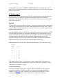


![Tutoriel Charte de la Diversité Mode d`emploi [Mode de compatibilité]](http://vs1.manualzilla.com/store/data/006524289_1-05943c8b39f7a218caf45e0c85aed489-150x150.png)