1
Introduction to FE Based
Fatigue Analysis
Using
MSC.Fatigue
© Copyright 2005 nCode International Ltd.
Introduction to the Problem
1
Ch1
Ch2
Input Forces
Ch3
Introduction
This guide takes a new user through a typical
FE based fatigue analysis. It describes each stage of
the process from viewing the FE model and stresses to
post-processing the fatigue results. The reader is
encouraged to undertake various sensitivity studies to
establish the adequacy of the component in fatigue.
The guide introduces two MSC programs:
MSC.Patran – MSC’s FE pre– and post-processor
MSC.Fatigue – MSC’s FE based fatigue solver
The Problem
You have to carry out a fatigue analysis on the front
shock tower of a new car. The FE department have
prepared the FE model and have obtained static stress
solutions for 3 loading directions as indicated in the
drawing.
The road load data department have provided
characteristic loading for some of the worst events.
The time signals have the equivalent damage of
approximately 200 miles (320 km) of normal driving.
The component should last at least 200,000 miles
(320,000 km) based on this harsh loading environment.
The component will behave quasi-statically.
© Copyright 2005 nCode International Ltd.
Some Program Basics Before We Start
FIN stands for
‘Fatigue INformation’ file
2
MSC.Fatigue accesses MSC.Patran groups
and stress/strain information, selects the
relative fatigue material from its own material database
and handles the time variation for all target locations at
once.
The analysis is submitted to the fatigue solver and the
damage results are recovered while leveraging on the
state of the art pre&post capabilities of MSC.Patran.
As a key component in your Virtual Product Development (VPD) process, MSC.Fatigue enables you to
quickly and accurately predict how long your products
will last under any combinations of time-dependent or
frequency-dependent loading conditions, and to
optimize your products for weight all within the familiar
MSC.Patran environment.
MSC.Fatigue supports all formats and codes
accessible by MSC.Patran including:
•
•
•
•
•
MSC.NASTRAN .op2 and .xdb
MSC.Marc .t16
ABAQUS .fil and .odb
FES stands for
‘Finite Element Stress’ results
Note:
The example case study is based on a real CAD
model donated by one of our valued customers. The
FE mesh, material property data and road load data
are, however, all fictitious and have been prepared
especially for this example.
ANSYS .rst
LS-Dyna .D3plot
© Copyright 2005 nCode International Ltd.
MSC.Patran – Viewing the FE Model and Stresses
Analysis | Access Results to import the FE
and results model file
Results | Create | Quick Plot to
Plot stress results
3
Linear static finite element analyses have
been performed already with three load
cases, each of magnitude of 1000 Newtons and the
model and results are contained in the results file,
shock.op2.
To begin, access this model and results information
into a new database using MSC.Patran. Note that all
instructions using MSC.Patran apply for MSC.Fatigue
Pre&Post users too.
Start the graphical interface and open a new database
from File | New and call it shock. The model was run
through an MSC.Nastran analysis, so keep the
Analysis Preference set to MSC.Nastran when asked.
Click on the Analysis toggle switch on the MSC.Patran
main toolbar. When the Analysis form appears, set the
Action to Access Results, the Object to Read Output2,
and the Method to Both (model and results). Press the
Select Results File button and select the file
shock.op2. Press the Apply button. The model will then
appear and you are ready to set up a fatigue analysis.
Before moving on to the fatigue analysis, first press the
Results application switch on the main form to view the
stress results from the MSC.Nastran analysis. The
Create | Quick Plot form is displayed. Go to the Select
Results Case listbox and select Load Case 1. Then
from Select Fringe Result listbox and select Stress
Tensor. Set the Quantity option menu to Maximum
Principal 2D. Press the Apply button and note the
areas of high stress. The maximum principal stress
appears to be about 62 MPa.
Middle mouse button to
Rotate model
© Copyright 2005 nCode International Ltd.
MSC.Fatigue – Set Up the Fatigue Analysis (1 of 8)
The analysis type offered depends
on the FE results available. For
linear static analysis, the options
include EN and SN, along with
various multiaxial methods.
Random Vibration Fatigue is
available if PSD results are used,
and Seam-weld and Spot-weld
options are also available.
For general analysis we recommend an EN approach first and
then decide whether a multiaxial
approach is required following an
inspection of the biaxiality plots.
We will discuss this later.
SN is not preferred for most FE
analysis because it is invalid in
regions of elastic-plastic stress
such as those adjacent to notches
and holes.
Most FE solvers pay no heed to
the units used provided they are
consistent. It is necessary,
however, for the fatigue solver to
know the original stress units
used in the FE analysis so it can
translate the appropriate
material data.
4
To begin setup for a fatigue analysis, from the
Tools pulldown menu in MSC.Patran, select
MSC.Fatigue and then Main Interface. This will bring
up the MSC.Fatigue main form from which all
parameters, loading and materials information, and
analysis control are accessed.
Once the form is open, set the General Setup
Parameters as shown.
Here we have a choice of Element or Nodal results. We would
usually recommend the ‘Element’ result option for shell elements as
this yields the most accurate stresses, however, we will choose the
‘Node’ option in this example.
In this case, we will use the stress results; however, the user can opt to use strain
if these are present. For linear analyses, (or non-linear where material hardening is
not considered), there’s no difference between taking stress or strain. However, if
you wish to include non-linear material behaviour in the FE analysis, you should
use the Strain results here, and select E-P Input (elastic-plastic).
Enter a Jobname and Title for this analysis here.
© Copyright 2005 nCode International Ltd.
MSC.Fatigue – Set Up the Fatigue Analysis (2 of 8)
The FE results file contains 6
component stresses or strains for
each element. These pertain to the
three axial and three shear
components. Principal stresses or
stress invariants (like Von-Mises)
can be obtained from the
components. This selection allows
the user to pick which stress property
to use for the fatigue analysis. In
general, the Abs. Max Principal
stress should be used as this yields
the best fatigue results.
Standard EN material properties are
applicable only for uniaxial stress
states. Where stresses are
proportional biaxial (e.g. plane strain,
torsion, etc.) a correction is required. I
would always recommend using the
Hoffmann-Seeger method for all
analyses.
If the stress state is non-proportional,
we must use a more complex fatigue
analysis. We investigate the stress
state in more detail later in the book.
Fatigue is influenced by
the residual stress field
in the component and
the mean stress of the
cyclic hysteresis loop.
Several methods are
available to account for
this, the default is taken
as the most popular
method.
5
Solution Parameters
Within the MSC.Fatigue main interface, open the
Solution Params... form. On this form, set the
parameters as shown.
Elastic-plastic correction
can be over-ridden if a
non-linear analysis of
material hardening is
carried out in the FE
analysis.
A degree of statistical scatter is usually observed in the fatigue properties of
materials. Many test labs provide the standard error coefficient to express this
scatter. If these data are available, the program allows the user to vary the
certainty of survival. A 50% COS describes the least-square fit through the data,
a 97.7% COS would represent the mean minus 2 standard deviations. The higher
the COS, the greater the confidence. It is recommended that 50% be chosen for
the first analysis run, followed by a sensitivity study on the influence of material
quality. Many data sources omit this value and usually give properties for the
mean minus 2 Standard Deviations. In this case, varying the COS will have no
effect on the results.
A factor of safety on stress overload can be computed. The user
enters the required life of the component and MSC.Fatigue will back
calculate to determine the allowable stress overload (Scale factor)
that can be withstood without compromising the fatigue life.
© Copyright 2005 nCode International Ltd.
MSC.Fatigue – Set Up the Fatigue Analysis (3 of 8)
6
Material Information
You now need to associate fatigue property
data for the various element groups used in the FE
analysis. Each group of elements can be assigned its
own fatigue properties, so welds could be associated
with a different property to that of the parent metal, for
example. This stage is necessary because the FE
solver knows nothing about the fatigue properties of a
material.
Existing default group
comprising of all entities
New group name
Ctrl
to select multiple items
The first step is to create a group which contains all the
shell elements of the finite element model. There are a
number of ways to substructure your model in groups.
For example, select Group | Create from the main
menu bar of MSC.Patran, change the Method to
Element/Topology, call the new group shells, and
select Quad4 and Tria3. Press the Apply button to
select the multiple items.
Note: MSC.Fatigue can only process locations
connected to shell or solid elements with available
stress results. This means the bar elements have to be
excluded from our fatigue analysis group.
Groups
This is an important feature in MSC.Fatigue. It is necessary to specify a group which
contains the nodes and/or elements for which you wish to perform a fatigue analysis.
In MSC.Patran, by default all elements and nodes are contained in the default_group.
However groups can be created to handle a reduced set of nodes/elements when the
model needs to be broken into more than one group for defining multiple combinations
of materials and surface finishes/treatments.
Creating a group is relatively straight forward and can be done in many automated
ways. Alternatively you can supply a name and graphically select entities from the
graphics screen or type them in the appropriate databox manually using the convention Node or Elem in front of any list of nodes or elements.
© Copyright 2005 nCode International Ltd.
MSC.Fatigue – Set Up the Fatigue Analysis (4 of 8)
7
Surface Finish and Treatments are
modelled using the Kf approach.
Kf values are published for various
finishes and are represented as a
function of material strength.
These values only apply to Steels
and should only be used for qualitative comparisons.
The strength reduction factor (Kf) is
used by fatigue engineers for modelling many effects such as notches,
surface finish and treatment, etc. It
acts by either scaling the stresses
prior to Neuber correction or rotating
the SN curve downwards, (for more
information please refer to the
Fatigue Theory Training course).
This option allows the user to enter
an additional Kf factor that will apply
to all elements in a group. This
function is useful in de-featured FE
analyses and for sensitivity studies
into quality of finish.
The default for this parameter is infinity which implies a Neuber elastic-plastic correction. When selecting the Mertens-Dittmann or Seeger-Beste methods, any
value greater than 1.0 may be defined. Only these methods use this parameter
and setting the parameter to infinity reverts this method back to the traditional
Neuber elastic-plastic correction. The shape factor or elastic strain concentration is
a function of the shape of the cross section of the component and the type of loading - see Elastic-Plastic Correction chapter in the User Manual.
Material Information
From the MSC.Fatigue main interface, open the
Material Info... form.
We now have to associate the element group properties with appropriate material fatigue properties (i.e. a
suitable EN curve)
•
Click on the first cell in the Selected Materials
Information: spreadsheet (1:Material) and pick
material SAE1008_91_HR from the list of
available materials in the standard materials
database
•
Click on Region column and select the shells
group
•
Leave all other options (Finish, Treatment, Kf,
Shape Factor and Multiplier) to their default
settings
These options allow you to apply
an additional Multiplier or Offset
value to all elements in the group.
The stress is first of all multiplied
by the Muliplier and then
summed with the offset.
In order to manipulate and view
all the available material
properties in the database,
press the Materials Database
Manager button to launch
PFMAT. Let us take a look at
materials we have used. Load
the material by pressing the
Load | data set 1 switch and selecting
SAE1008_91_HR from the list. Press or double click
Graphical Display | Strain life plot to view the strain-life
curve for this material.
© Copyright 2005 nCode International Ltd.
MSC.Fatigue – Set Up the Fatigue Analysis (5 of 8)
Loading can be in the
form of constant
amplitude or variable
amplitude. Constant
amplitude loads are
entered directly using
Wave creation. Variable
loads are represented by
a time signal file in either
nCode DAC or MTS
RPCIII format. (ASCII
files can be translated if
required). Variable loads
are loaded to the
database using Load
files.
Add a description to the Loading
Database manager of each time
history file here, and then set
Load type and Units to Force
and Newtons respectively.
In order to report fatigue life in
units which are more appropriate
for the component or structure
being analysed, it is required to
enter both the number of units
and unit type here which describes the duration of the
loading.
8
Loading Information
Now in order to do a fatigue analysis using linear static
FE results we must define how the loads vary with
time. This is easily done in MSC.Fatigue using the
Loading Database Manager, PTIME.
Open the Loading Info... form on the MSC.Fatigue
main interface. Then press the Time History Manager
button. This will launch PTIME.
PTIME is a loading (time series, histogram, PSD)
database manager which has been designed to enable
the MSC.Fatigue user to manipulate and manage time
history and other data file types. The time history and
other loading type files are not loaded into the
database, but are resident in the local working
directory together with the ptime.adb file which
contains the associated database data for each loading
file.
In this case, Load files, browse for the first time
histories, load01.dac, and complete the options as
shown. Repeat this for load02.dac and load03.dac.
Note:
MSC.Patran will be suspended during this operation
until PTIME is closed. This is indicated by the blue
busy signal in the top right corner. Since PTIME is a
separate process, this suspension is necessary to
make MSC.Patran’s graphical interface recognize any
new time signals.
© Copyright 2005 nCode International Ltd.
MSC.Fatigue – Set Up the Fatigue Analysis (6 of 8)
9
Loading Information (continued)
Multi-file Display - to look at the time variations of the
three load cases, use the Multi-channel... | Display
Histories option. This will run the multi-file display
module, MMFD. When MMFD appears, use the list
facility to select the four files above (use the Shift key
to make multiple selection from the file browser). Note
that the files will not appear in the databox but the
number of files selected will appear below it. Accept all
the other defaults on the form and press OK. The files
will be displayed.
The Multi-file Display provides summary
data for each time history, such as
sample rate, number of points, and
maximum and minimum values.
Note:
If you make a mistake selecting the files for multi
channel display, you can always add to or delete from
the currently selected list. Simply press the list button
again and a menu will appear allowing you to make
modification to the list of files. If you are already in
graphical display, select File | New File(s) to return to
the file selection screen.
© Copyright 2005 nCode International Ltd.
MSC.Fatigue – Set Up the Fatigue Analysis (7 of 8)
Fatigue life is usually
expressed as the number of
repeats of a time history
required to fail the component. It is often desirable to
express this in more meaningful units, such as miles.
Therefore the user can
specify that 1 repeat is
equivalent to x miles, for
example. Set to 1 repeat =
200 miles (or 320 km).
A single linear FE analysis
could be used to perform
fatigue analyses at different
stress levels. MSC.Fatigue
will use the load magnitude
to divide all the stress
results before scaling them
according to the time
signal file.
If shell elements are used in the FE model you can
choose whether to use the top or bottom surfaces.
In this example, select Z1 layer for all load cases - this is
the bottom shell surface results.
10
Loading Information (continued)
Fill out the spreadsheet on the Loading Info...
form; the spreadsheet is used to establish the
association between the load histories (the time
variation of the load) and the FE load cases.
MSC.Fatigue scales and combines the stress distributions according to the time histories, to obtain the
stress history for each node.
Set the Number of Static Load Case to 3 and press the
Return or Enter key to effect the change. Place the
cursor in the cell in the first column and click the
mouse button. This selects the cell. A number of
listboxes, buttons, and pulldown menus appear below
the spreadsheet. This is where you specify the FE
analysis results that you will use in the fatigue analysis.
They appear empty at first. To fill them, press the Get/
Filter Results... button. On this form turn the Select All
Results Cases toggle ON and press the Apply button.
This will fill the listbox on the left with all available
result load cases in our MSC.Patran database. Make
sure that the Fill Down toggle in the middle of the form
is set to ON and select the first available loadcase. In
the now populated second listbox select Stress Tensor
as your tensor option and then press the Fill Cell
button. Fill in the remaining columns as shown.
Note:
The spreadsheet is filled out in exactly the same manner as with a single load. With
multiple load cases however, it is only necessary to Get/Filter Results... once. Each
subsequent time you fill in a cell with a load case ID, all results remain in the selection
listbox. Also note that the actual load case IDs may vary from what is shown in the table.
© Copyright 2005 nCode International Ltd.
MSC.Fatigue – Set Up the Fatigue Analysis (8 of 8)
11
Calculate Normals
These averaged nodal
outward normals are
also graphically plotted
for visualisation and
verification purposes.
Press the Remove
Vectors button to remove them. Once they
have been removed
they can only be replotted if the whole procedure is repeated.
Within the MSC.Fatigue main interface, open the Job
Control... form. The Calculate Normals option is an
essential precursor to running the biaxiality analysis if
you know your results are not surface resolved (znormal is not zero). This routine determines surface
normals at each surface node, and writes them to the
file jobname.vec. MSC.Fatigue detects the presence of
this file and uses it to define a local coordinate system
at each surface node that has its z-axis normal to the
surface. The stress results in the fatigue analysis input
file are then written in this coordinate system, permitting the software to carry out a biaxiality analysis in the
x-y plane only.
You can read about calculating normals in the
MSC.Fatigue Quickstart Guide, Chapter 11 “A
Multiaxial Assessment”.
Note:
If you view the component of the stresses normal to the surface, you will note that these are very
close to zero over the majority of the model (the exception being the loading points as would be
expected). A good look at these stresses would reveal model quality. By calculating normals in
MSC.Fatigue, the results are expressed as surface resolved stresses, meaning the two major
principal stresses lie in the plane of the surface with the third principal stress being zero (normal to the
surface). This is important for models with solid elements especially given that 99% of cracks initiate
on the surface.
The main reason that we need surface resolved stresses is for the biaxiality analysis to properly
calculate the biaxiality ratio which will be discussed later in this example. Without surface resolved
stresses it would be difficult, if not impossible, to assess the multiaxial stress state of the component.
© Copyright 2005 nCode International Ltd.
MSC.Fatigue – Running the Fatigue Solver
12
Select Monitor Job to
view the progress of the
analysis run
You are now ready to run the fatigue analysis.
Open the Job Control... form. Set the Action to
Full Analysis and press the Apply button. The database
will close momentarily as the results information is
extracted. When the database reopens, the job will
have been submitted. You can then set the Action to
Monitor Job and press the Apply button from time to
time to view the progress. The solution should only
take a minute or so to complete. When the message
”Safety factor analysis completed successfully”
appears, the analysis is complete. Close down the Job
Control... form when done, and then open the
Results... form on the main MSC.Fatigue setup form
(not to be confused with the Results application switch
on the MSC.Patran main toolbar). With the Action set
to Read Results press Apply. The fatigue analysis
results will now be read into the MSC.Patran database
and then be accessed as any other FE result.
Select Read Results to
read the fatigue analysis
results into the MSC.Patran
database for postprocessing.
© Copyright 2005 nCode International Ltd.
MSC.Patran – Viewing the Fatigue Damage Contour
13
Just as you viewed the stresses earlier, you
can view the damage and life plots. Select the
Results application switch on the MSC.Patran toolbar.
The Create | Quick Plot form will appear. On this form
select the Crack Initiation, shockfef item in the Select
Result Cases listbox and the Log of Life (Cycles) item
in the Select Fringe Result listbox and then press
Apply.
Note that the smallest life reported is approximately
5.62. This is a log base(10) value. So the actual life
value is 105.62 which is about 400,000 miles.
Look at the Damage, and Factor-of-Safety plots in the
same way (use Factor of Safety, shockfos in the Select
Result Cases listbox for factor of safety).
Reporting life values in log units tends to spread the
contour bands out for better results interpretation.
Since such a large spread of results values can occur
(from finite to infinite at locations where no damage
occurs), it is not really practical to plot pure life values.
Life
400,000 Miles
Min Factor of Safety = 1.28
Click this button,
Fringe Attributes, to
change the contour
plot settings, such as
style and shading
© Copyright 2005 nCode International Ltd.
Introduction to Sensitivity Analysis
Is the FE analysis adequate?
14
Does the multiaxial load cause a multiaxial
stress state at the critical region?
You have now carried out your first
MSC.Fatigue analysis. You have a nice
contour plot showing where the component is likely to
fail and have determined an estimated fatigue life of
400,000 miles with a Factor of Safety on overload of
1.2. At the moment everything is looking fine.
But are you sure?
Sensitivity Analysis
In the next few frames we will conduct a sensitivity
analysis on the component to determine whether a
non-proportional multiaxial analysis is required, we will
investigate the effect of residual stresses caused by
cold forming and we will look at the quality of the FE
mesh.
How would residual stresses caused by cold
forming affect the fatigue life?
© Copyright 2005 nCode International Ltd.
Mesh Quality
15
Notice high gradient of damage relative to mesh size
Select the Results application switch on
MSC.Patran toolbar. On the Create | Quick
Plot form select the Total Life, shockfef item in the
Select Result Cases listbox and the Damage item in
the Select Fringe Result listbox and then press Apply.
Fringe Attributes button
Select Fringe Attributes button and set Fringe Edges |
Display to Element Edges. You can also change the
legend colours using Spectrum… (the one used in
these plots is hotcold12).
Zoom-in to the critical area and notice how coarse the
mesh is relative to damage gradient.
Look at the stress results by selecting each load case
and changing the display to view the Von-Mises plot.
Notice Von-Mises stress gradient over the critical element ~112MPa to
~60MPa!
Smooth contoured Fringe plots can hide many sins if you don’t know how
to look for them.
If element stresses are chosen for the Results Loc on the General Setup
Parameters form, the contour plots are all displayed as colour patch plots.
These are less attractive than the fringe plots but show poor meshing in a
much more apparent fashion. You may wish to re-run this tutorial from
Frame 4 using ‘Element’ results instead of ‘Node’ if you have time when
you’ve finished.
© Copyright 2005 nCode International Ltd.
Mesh Quality & Stress State Analysis
16
Multiaxial Check
We commonly talk of three types of stress state.
1 Uniaxial – has only 1 principal stress which changes in magnitude but not direction
2 Proportional biaxial – has 2 principal stresses which change proportionally in magnitude but do not change
in direction
3 Non-proportional biaxial – has 2 principal stresses that can vary non-proportionally in magnitude or direction
Measured Fatigue curves (SN & EN) pertain to Uniaxial stresses only. Biaxiality corrections (like HoffmannSeeger) extend these results so they can be applied to most Proportional biaxial stresses. Non-proportional
biaxial stresses are very rarely located in regions of high fatigue damage, however, if you are unfortunate
enough to encounter them, you will have to switch to a multiaxial fatigue model (like Wang-Brown) for these
elements.
Multiaxial fatigue models require longer computation time that the others, so most users start by assuming
uniaxial (or proportional biaxial) conditions and then check the stress states in the critical regions to see if the
assumption is valid. If a non-proportional state is encountered, then a multiaxial analysis is conducted on a small
subset of elements.
In this frame we will investigate the stress state of the critical nodes and determine whether a multiaxial analysis
is required.
Back on the main MSC.Fatigue toolbar, press
the Results... toggle, change the Action to List
Results and hit Apply. This will start the module
PFPOST which lists the fatigue analysis results in
tabular form. Accepting the jobname and the default
filtering values, by pressing OK a couple of times, will
get you to the main menu. Press or double click the
Most damaged nodes switch to view a tabular listing.
See discussion of results on this page...
Multiaxial Rules of Thumb:
FE Mesh Quality and Convergence
Hoffmann-Seeger method is
adequate where:
Fatigue damage is exponentially related to the stress range
and so we would expect to see lower convergence between
neighbouring nodes than would be observed with stress results. However, we would still usually expect much less than a
factor of 2 in life between neighbouring nodes. Isolated hot
spots of damage like those observed here are indicative of
singularities or poor stress meshing like that seen in the previous frame.
1
2
3
SD Ratio < ~0.1
Mean Ratio < ~0.3
Ang. Spd. < ~10°
Node 27386 may be
questionable in this case!
For more information on Multiaxial Fatigue Analysis, please
refer to the Users Manual or the ‘Fatigue Theory’ training
course.
© Copyright 2005 nCode International Ltd.
The Effect of Residual Stresses
17
Offset can be used to
model the residual
stresses arising from
cold forming. Determining the actual residual
stresses is a fairly costly
undertaking involving
prototype testing or nonlinear FE analysis. In this
analysis we apply the
most pessimistic residual
stress, that of yield in
tension, and determine
whether this would
unduly compromise the
component.
Subsequent sensitivity studies
need only be conducted on the top
few nodes. In this case we have
chosen the top 3.
Firstly, create a new group of the top 3 nodes.
Use the Group | Create | Select Entity, New
Group Name worst, and enter Node 31114 26994
27386.
Return to the MSC.Fatigue main interface.
Open the Material Info... form and click on the Region
box for material 1. Select the new worst group. Then
move the slider to the right to show the Offset box.
Click this box and enter Offset Value: 253 (this is the
yield stress of the material). Press Enter to apply this
offset and then OK to close the form.
Open the Job Control... form. Set the Action to Full
Analysis and press the Apply button.
Fatigue life is not reduced significantly (~10%) with residual stress,
therefore a costly residual stress
calculation is not required
© Copyright 2005 nCode International Ltd.
Conclusions
18
Congratulations, you have run your first MSC.Fatigue analysis.
This is just one type of analysis that can be done.
Analysis Conclusions
Design Life = 200,000 Miles
Estimated Fatigue life = 400,000 Miles , ∴ OK.
(Factor of 2 on life)
Supported FE Results
General Fatigue Models
Permissible overload / safety factor = 1.2, ∴ OK.
•
•
•
•
•
•
•
Shells, Solids, Bars (Spot weld)
Stress or Strain
•
•
Linear Static and Quasi-static
Transient Dynamic
Modal Transient
Random Vibration (PSD)
Non-linear
Local Strain Life (EN)
Multiaxial EN (numerous methods
including Wang-Brown and
Fatemi-Socie)
•
•
Nominal Stress Life (SN)
•
Dirlik Vibration Fatigue
Multiaxial SN (including Dang-Van
and McDiarmid)
Weld Fatigue Models
•
•
•
BS7608 SN approach
Sensitivity to residuals = ~10%, 380,000 Miles, ∴ ok.
Convergence on stress = (112-60)/60 = 87% error,
VERY POOR!
Convergence on Life = VERY POOR!
% Certainty of Survival = insufficient material data (No
std. error given in material data)
Multiaxiality study = Critical nodes are proportional but
some nodes have biaxiality > 0.3. ∴ a multiaxial
assessment will be required when better FE results are
available.
LBF Spot Weld approach
Volvo/LBF Seam Weld approach
COMPONENT NOT PROVEN!
Requires better FE model.
© Copyright 2005 nCode International Ltd.
For further details ...
To find your local nCode or MSC.Software office, or to learn more about the companies
and products, please contact:
'
nCode International
+44 114 275 5292
[email protected]
- www.ncode.com
nCode International Inc.
+1 248 350 8300
[email protected]
19
MSC.Software Corporation
+1 714 540.8900
+1 800 642.7437 ext. 2500 (U.S. only)
+1 978 453.5310 ext. 2500 (International)
- www.mscsoftware.com
MSC.Software GmbH
+49 89 43 19 87 0
! "#
$ %
&
MSC.Software Japan Ltd.
+81 3 3505 0266
© Copyright 2005 nCode International Ltd.
20
Notes:
© Copyright 2005 nCode International Ltd.