Download 1 Introduction 2 Background Theory

A Graphical User Interface to
Generalized Linear Models in matlab
Peter K Dunn
July 12, 1999
Abstract
Generalized linear models unite a wide variety of statistical models in a common theoretical framework. This paper discusses glmlab|software that enables such models to be tted in the popular
mathematical package matlab. It provides a graphical user interface to the powerful matlab computational engine to produce a program that is easy to use but with many features, including osets, prior
weights and user-dened distributions and link functions. matlab's graphical capacities are also utilized
in providing a number of simple residual diagnostic plots.
1 Introduction
Generalized linear models (or glm's) were introduced by Nelder and Wedderburn [8] in 1972 as a means of
unifying a diverse range of statistical models, including multiple regression, log-linear analysis and probit
analysis. The subsequent release of the Glim software (Francis et. al. [4]) enabled the theory to be applied
easily to practical problems. Since that time, other popular statistical software packages, including S-Plus
(Statistical Sciences [10]) and SPSS (Norusis [9]), have incorporated glm's.
This paper explores the use of matlab (The MathWorks Inc. [5]) to implement glm's using a graphical
interface in the program glmlab. The motivation for the development of the program comes from the need
to teach a short course in statistical models, with a section on glm's, to a wide cross-section of students:
dierent students may be familiar with dierent packages, and perhaps some students not familiar with any
statistical package at all. All have a rm grounding in matlab, however. There are many advantages with
this approach: the rich variety of mathematical and graphical functions of matlab are readily available;
there is no need to purchase or learn a specialist statistics package (such as Glim); the same code can be
used for all the dierent matlab platforms; the graphical environment makes glm's quickly available to
students in a short course. The software is not intended to take the place of commercial packages, but rather
to bring the world of glm's to users of matlab.
Section 2 provides a theoretical background to glm's. Section 3 discusses some of the methods used in
the software. The program itself is discussed in Section 4, and two examples are discussed in Section 5.
Section 6 briey concludes with a short discussion.
2 Background Theory
Generalized linear models are based around distributions in the exponential family, such that
fY (yi ; i ; ) = a(yi ; ) exp [fyi i ; (i )g=]
(1)
for known functions a() and (). In such models, i = 0 (i ) and Var(yi ) = V (i ), where V (i ) = 00 (i )
is known as the variance function and is the dispersion parameter. The linear predictor, usually referred
to as , is given by = XT .
The mean parameter, , is related to the linear predictor, through a monotonic, dierentiable link
function so that gi (i ) = i . (Usually, the link function is the same for all points i = 1; : : : ; n.) The link
function can be chosen independently of the distribution, but a popular link function (called the canonical
link function ) is found by setting i = i . The standard multiple linear regression technique sets the link
function at = . Distributions of the form (1) include the normal (Gaussian), inverse Gaussian, gamma,
Poisson and binomial distributions.
1
The deviance of a model (a measure of the distance between y and ) is given by
D(yi ; i ) =
n
X
i=1
where d(yi ; i ) is the unit deviance dened as
di (yi ; i ) = 2
Z
wi d(yi ; i )
yi
i
yi ; u du;
V (u)
and wi are prior weights.
The X matrix can contain quantitative variables and also qualitative variables (also called categorical
variables, or factors ). Each level of the factor is identied with a variable. However, there are usually
dependencies between the variables. This overparameterization introduces a singular design matrix which
must be removed prior to the tting of any model. There are many dierent methods available for doing so,
including Helmert contrasts (as favoured by S-Plus), orthogonal polynomials, sum-to-zero constraints and
corner-point parameterizations (as in Glim). All are dierent methods of introducing qualitative variables
by having k ; 1 independent variables for a variables with k levels.
The theory of glm's has been documented by Nelder and Wedderburn [8], McCullagh and Nelder [6] and
more briey by Dobson [2] among others.
3 Methods
The algorithms for tting glm's to data are well established and robust (see McCullagh and Nelder [6] and
Nelder and Wedderburn [8]). The maximum likelihood estimates of can be found using iterative least
squares: set 0 = XT 0 to be the initial value of the linear predictor, and 0 the corresponding value of the
tted value (recall that = g()). The link function is linearized so that
^
^
z0 = 0 + (y ; 0) dd
0
and is then regressed onto the covariates X with quadratic weights dened as
d ;
1
W0 = d V (0 )
to produce a new estimate of . The algorithm is repeated until convergence.
Starting values for the algorithm are easily obtained from the data. Setting 0 = y, ^0 is then obtained
from the link function. In some cases, the method needs some rening (for example, to avoid calculating
log 0 when tting a log-linear model with zero counts).
The program itself|called glmlab|consists of numerous m-les (matlab functions and scripts) for
tting generalized linear models. Large portions of the code involve setting up the graphical interface,
parsing the input strings and subsequent checks of the inputs, and executing menu commands. The example
pieces of code included in the Appendices concern the actual tting of the model (the code probably of most
interest to readers of this paper). The actual tting algorithm is implemented in the le irls.m as shown
in Appendix A.
Each distribution used in the program has an associated le that contains the information relevant to
glmlab; namely the variance function and the deviance (see Appendix C for an example of the gamma
distribution). Similarly, each link function has an associated le containing information about the link;
namely nding given ; nding given ; and nding d=d given . An example using the probit link
function is given in Appendix D. This idea of placing relevant information about distribution and links in
les enables the user to create new distributions and link functions with a minimum of knowledge of matlab
programming.
Parameters such as the maximum number of iterations, the parameter accuracy and the ill-conditioning
tolerance, can be altered from one of the drop-down menus on the main screen.
The program produces an output le called DETAILS.m that contains information about the variables
tted, and deviance from each model; see Section 5. Screen output gives information such as parameter
estimates and residual deviance. This information is easily captured using the matlab diary command.
2
Figure 1: The Main glmlab Window
4 The Program
There are many functions written for the analysis of particular statistical problems in matlab, including a
subset of problems in the generalized linear models framework. However, even with the Statistics Toolbox,
matlab lacks a procedure for analysing the full range of generalized linear models.
This section discusses the program glmlab that has been written to allow matlab to analyse such
situations. glmlab uses a graphical interface and so is easy to learn and use. Among other features, it
allows the user to add distributions and link functions that are not included, and save and load work between
sessions. It does not require the user to have access to the Statistics Toolbox.
Some aspects of the program are listed below.
4.1 Data Entry Windows
There are four areas in the main screen (see Figure 1) for the entry of data or variable names:
Response (y): The response (or y) variable is entered here (but see Sections 4.6 and 5.2 also).
Covariates (X): The covariates, or X-matrix, is entered here. The constant (or intercept) is automatically tted, but this can be altered by the user in the Options menu.
Prior Weights: Any prior weights can be entered here (for example, in a weighted regression, to omit
structural zeros, or optionally with the binomial distribution as in Section 5.2).
Oset: Any oset variables are entered here. An oset is a variable with a known coecient (see
Section 5.1).
Valid matlab workspace variables can be entered, as well as most valid matlab commands that produce
matrices of the correct type and size. For example, the user could enter magic(4) as the covariates, and
[1.0, 3.2, -1.2, 0.5]' as the response. Some commands, especially if complex, will not work. Using
vector variables dened in the matlab workspace is recommended.
4.2 Menu Items
There are eight menu items in the main glmlab window (see Figure 1):
File: The le menu opens data les (*.mat les); loads and saves models (*.glg les); exits from
glmlab; quits matlab.
3
Error
Distribution
Default Link
Function
Default Scale
Parameter
Normal
Identity
Mean Deviance
=
Inverse Gaussian Inverse Quadratic Mean Deviance
= 1=2
Poisson
Logarithm
Fixed (at 1)
= log Binomial
Logit
Fixed (at 1)
= log[=(1 ; )]
Gamma
Reciprocal
Mean Deviance
= 1=
Table 1: Default Settings for Chosen Distributions
In the table, is the linear predictor and is the mean (or in the binomial case).
Distributions: In the distributions menu, the user selects the distribution of choice. There are ve
built-in distributions (normal, inverse Gaussian, gamma, Poisson, binomial). Users can also add their
own distributions which will appear in the menu. Distributions have default link functions and scale
parameters as shown in Table 1.
Link: In the link menu, the user selects the link function of choice. There are eight built-in link
functions (identity, log, square root, power, reciprocal, complementary log-log, probit and logit (or
logistic)). Users can also add their own links which will appear in the menu. For each distribution,
the default link function is the canonical link (see Table 1).
Scale Parameter: The scale parameter can be set to a xed (positive) value, or to be estimated by the
mean deviance.
Residual Type: Three types of (standardized) residuals can be chosen: deviance, Pearson and quantile.
(See Dunn and Smyth [3] for a description of quantile residuals.)
Options: Many options can be set, including recycling tted values, restoring default options, declaring
new models, including the constant term (intercept) in the t, and changing the tting parameters.
Plots: After tting a model, six dierent plots are available directly from glmlab:
{ Residuals vs Response;
{ Residuals vs Covariates (X);
{ Normal Probability Plot;
{ Residuals vs Fitted Values;
{ Residuals vs Transformed Fitted Values: The transformation is to the constant information scale of
the distribution; see Nelder [7] and McCullagh and Nelder [6];
{ Fitted Values vs Quantile Equivalents.
Of course, using matlab's facilities and the variables returned by glmlab into the matlab workspace
(see Section 4.5), numerous plots can be constructed.
Help: Contains help screens, plus links to the glmlab Home Page and on-line manual, and a simple
demonstration. By having a quick link to the on-line manual, users have timely help at their disposal.
The manual can be found at http://www.sci.usq.edu.au/staff/dunn/glmlab/glhtml/html/gli.
html. The glmlab Home Page can be found at http://www.sci.usq.edu.au/staff/dunn/glmlab/
glmlab.html
4
4.3 Buttons
There are seven buttons in the main glmlab window (see Figure 1); three of these along the bottom are of
the most interest.
New Model: Pressing this button prepares glmlab for tting a new model by restoring default settings
and clearing variables.
Fit Specied Model: Pressing this button ts the model as currently specied.
Quit glmlab: Quits glmlab.
The remaining four buttons on the left of the main window (for example, one is labelled Response (y):) open
windows for selecting numeric variables from the workspace.
4.4 Commands
There are only a few commands that need to be learnt to use glmlab:
glmlab: Once in matlab, the user starts the program by typing glmlab at the matlab prompt.
fac: The fac command is used to ag a variable as qualitative (see Section 5.1). fac uses a cornerpoint parameterization (as in Glim) that includes each level of the factor as a dummy variable, and
excludes the rst column to preserve full-rank.
@: The @ symbol is used to ag interactions between variables (see Section 5.1).
makefac: The makefac command is similar to the Glim command %gl. It allows for easier creation of
factors. To create a factor of length 36 that has twelve levels (A; B; C; : : : L say), occurring in groups
of three (that is, A, A, A, B , B , B , C , : : :, K , L, L, L), the variable can be generated using
Newvar = makefac( 36, 12, 3 );
in the matlab workspace.
4.5 Returned Variables
After the tting of a model, ten variables are made available in the matlab workspace:
BETA: The parameter estimates;
SERRORS: The standard errors of the parameter estimates;
FITS: The tted values;
RESIDS: The residuals;
COVB: The covariance matrix of the parameters;
COVD: The covariance matrix of the dierences between parameters;
DEVLIST: The deviance at each iteration of the t;
LINPRED: The linear predictor, ;
XMATRIX: The X matrix used in tting the model;
XVARNAMES: The names of the X-variables.
4.6 Binomial Responses
Binomial responses variables require some special handling. Three link function are unique to the binomial
distribution (and are unavailable otherwise from the Link menu): the logit (or logistic), probit and complementary log-log link functions. In addition, the response variable must reect the binomial situation of
counts and sample size. In this situation, response variable consists of two columns: the rst for the counts,
and the second for the sample sizes. (Note that this is dierent than the convention adopted in S-Plus, where
the response has the two columns as the number of successes and the number of failures.) When the data to
be analysed is in the form of probabilities, only one column is needed. See Section 5.2 for an example using
the binomial distribution.
5
/glmlab
/glmlab/fit
/glmlab/fit/dist
/glmlab/fit/link
/glmlab/plotting
/glmlab/misc
/glmlab/glmhelp
/glmlab/glmlog
Contains general information and les used in starting glmlab.
Contains numerous les for tting the model and parsing the input.
Contains information about the distributions that can be used.
Contains information about the link functions that can be used.
Contains plotting routines.
Contains other miscellaneous les used in glmlab, including formatting and tricks.
Contains the glmlab help menu information.
Contains log les, tting parameters, and data les that come
with glmlab.
Table 2: The Structure of glmlab
4.7 Directory Structure
glmlab consists of over 70 matlab les in a number of directories (or folders). They are structured as
shown in Table 2.
5 Examples
5.1 Ship Damage Data
McCullagh and Nelder [6, x6.3] give some data concerning wave damage done to cargo carrying ships,
available in the le shipdam.txt. The data consists of ve variables:
Ship Type: Five types of ship are considered (matlab variable Shiptype);
Year of Construction: 1960{1964, 1965{1969, 1970{1974, 1975{1979 (matlab variable Yearmade);
Period of Operation: 1960{1974; 1975{1979 (matlab variable Operation);
Aggregate Months of Service (matlab variable Service);
Number of Damage Incidents (matlab variable Damage).
The rst three variable are qualitative factors.
The data contains many interesting features that serve to demonstrate features of the glmlab software.
For example, there are many structural zeros, since (for example) ships made after 1975 cannot have periods
of operation before 1975. There is also an observational zero in the data. The authors consider an initial
model of the form
log(expected number of damage incidents)
= 0 + log(aggregate months of service) + (eect due to ship type)
+ (eect due to year of construction) + (eect due to service period):
(2)
The rst term after the intercept is a quantitative variable with a known coecient of 1. Such a variable
is known as an oset. As is usual with count data, the authors decide to use the Poisson distribution with
the logarithm link function. They expect overdispersion due to expected inter-ship variability and so we
over-ride the default xed scale parameter option in glmlab and estimate with the mean dispersion.
To t the model discussed in McCullagh and Nelder [6], variables are entered as shown in Figure 2.
Note that the oset variable is entered as log(Service); this shows that glmlab can happily accept
transformations being entered as variable names. log(Service) has been used as the oset because of the
model in Equation 2 proposed by McCullagh and Nelder. The variable Weights is a vector of prior weights
that omits the structural zeros (it is zero for the structural zeros, and one elsewhere). The following options
are also set:
To declare the distribution, choose Poisson from the Distribution menu.
6
Figure 2: Variables Entered for the Ship Damage Example
The logarithm link function is the default for the Poisson distribution (it is the canonical link), so no
changes need to be made using the Link menu.
To alter the scale parameter, choose Mean Deviance from the Scale Parameter menu. (For the Poisson
distribution, the Scale Parameter, by default, is set to a Fixed Value of 1.)
On pressing the Fit Specied Model button, results are presented on the screen as shown below:
>> === INFO :-| ========================================================
Response Variable:
[Damage]
Covariates:
fac(Shiptype),fac(Yearmade),fac(Operation)
- fitting a constant term/intercept
Offset Variable:
log(Service)
Prior Weights Variable: Weights
-----------------------------------------------------------Estimate
S.E.
Variable
------------------------------------------------------------6.405902
0.270524
Constant
-0.543344
0.220941
Shiptype(2)
-0.687402
0.409369
Shiptype(3)
-0.075961
0.361511
Shiptype(4)
0.325579
0.293459
Shiptype(5)
0.697140
0.186170
Yearmade(2)
0.818427
0.211217
Yearmade(3)
0.453427
0.290089
Yearmade(4)
0.384467
0.147143
Operation(2)
-----------------------------------------------------------Deviance:
38.695052
(change:
-39.883544)
Residual df:
25
(change:
-5)
Scale parameter (dispersion parameter):
1.547802
Output variables: BETA SERRORS FITS RESIDS COVB COVD
DEVLIST LINPRED XMATRIX XVARNAMES
The results, naturally, agree with those given in McCullagh and Nelder [6]. Variables with numbers
following are qualitative variables; the numbers refer to the levels of the variable. They are understood to
be in reference to the rst level of the variable, the same way in which Glim treats qualitative variables.
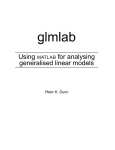
After a model has been tted, the Plots menu becomes available, and residual plots can be generated
to informally examine the residuals. For example, if deviance residuals were chosen from the Residual Type
menu, the Residuals vs Transformed Fitted Values plot is displayed on the screen; see Figure 3.
To include an interaction term between (say) Year of Operation and Year of Construction as a covariate,
enter the variables into the main window as shown in Figure 4. Pushing the Fit Specied Model button
produces the following output:
7
Figure 3: The Deviance Residuals vs the Transformed Fitted Values for the Ship Damage Data
INFO :-| ========================================================
Response Variable:
[Damage]
Covariates:
fac(Shiptype),fac(Yearmade),fac(Operation),fac(Yearmade)@fac(Operation)
- fitting a constant term/intercept
Offset Variable:
log(Service)
Prior Weights Variable: Weights
-----------------------------------------------------------Estimate
S.E.
Variable
------------------------------------------------------------6.515032
0.299392
Constant
-0.546126
0.225026
Shiptype(2)
-0.689259
0.416861
Shiptype(3)
-0.076216
0.368217
Shiptype(4)
0.321635
0.298830
Shiptype(5)
0.860880
0.253208
Yearmade(2)
0.972409
0.312793
Yearmade(3)
0.280620
0.330341
Yearmade(4)
0.668061
0.305957
Operation(2)
-0.387270
0.376715
Yearmade(2)@Operation(2)
-0.340986
0.404893
Yearmade(3)@Operation(2)
0.000000
aliased
Yearmade(4)@Operation(2)
-----------------------------------------------------------Deviance:
36.907591
(change:
-1.787460)
Residual df:
23
(change:
-2)
Scale parameter (dispersion parameter):
1.604678
Output variables: BETA SERRORS FITS RESIDS COVB COVD
DEVLIST LINPRED XMATRIX XVARNAMES
The nal parameter is aliased, in that it contains no information that is not already contained in the
other variables.
5.2 Example: Binomial Data
Because of the particular nature of the binomial distribution, a simple example is considered here. The data
comes from Bliss [1] (cited in Dobson [2]) and is shown in Table 3. The data involves counting the number
of beetles killed after ve hours of exposure to various concentrations of gaseous carbon disulphide (CS2 ).
The analysis concerns estimating the proportion ri =ni of beetles that are killed by the gas.
The variables in matlab were named Dose, Number and Killed for the obvious variables. Dobson
analyses the data using a logit link function. The data is entered into glmlab as shown in Figure 5. In
particular, take note of the entry for the response variable, which is entered as two columns. After choosing
8
Figure 4: Fitting Interaction Terms
Dose
Number of Beetles Number of Beetles
(log10 CS2 mg l;1 )
(ni )
Killed (ri )
1.6907
1.7242
1.7552
1.7842
1.8113
1.8369
1.8610
1.8839
59
60
62
56
63
59
62
60
Table 3: Beetles Mortality Data
9
6
13
18
28
52
53
61
60
Figure 5: Variables Entered for the Beetle Mortality Example
the binomial distribution and the logit link function from the menus, the results are given below:
=== INFO :-| ========================================================
Response Variable:
[Killed,Number]
Covariates:
Dose
- fitting a constant term/intercept
-----------------------------------------------------------Estimate
S.E.
Variable
------------------------------------------------------------60.717455
5.180701
Constant
34.270326
2.912134
Dose
-----------------------------------------------------------Scaled deviance:
11.232231
Link: LOGIT
Residual df:
6
Distribution: BINOML
Scale parameter (dispersion parameter):
1.000000
Output variables: BETA SERRORS FITS RESIDS COVB COVD
DEVLIST LINPRED XMATRIX XVARNAMES
The results agree with those given in Dobson. An alternative method is to t the model using the
probabilities ri =ni as the response (that is, one column of probabilities), and use ni as the prior weights.
The parameter estimates are identical. The residual plotted against the tted values (produced using the
Plot, Residual vs Fitted Value option) in Figure 6 shows a possible curvature.
6 Discussion
The program glmlab has been discussed for using matlab to t the wide class of statistical models known
as generalized linear models. The software is not meant to replace commercial packages, but to provide
matlab with facilities for dealing with such a class of models. While glmlab may not be as powerful
as programs like Glim and S-Plus, it oers an easy to use introduction to generalized linear models in a
user-friendly and powerful environment. It allows many dierent types of models to be tted, including
common models such as logit models, ANOVA, and multiple regression.
References
[1] C. I. Bliss. The calculation of the dosage-mortality curve. The Annals of Applied Biology, 22:134{167,
1935.
[2] Annette J. Dobson. An Introduction to Statistical Modelling. Chapman and Hall, 1983.
10
Figure 6: Residuals Versus Fitted Values for the Beetle Mortality Example
[3] Peter K. Dunn and Gordon K. Smyth. Randomized quantile residuals. The Journal of Computational
and Graphical Statistics, 5:1{10, September 1996.
[4] Brian Francis, Mick Green, and Clive Payne. The GLIM System: generalised linear interactive modelling. Release 4 Manual. Clarendon Press, 1993.
[5] The MathWorks Inc. MATLAB Reference Guide, August 1992.
[6] P. McCullagh and J. A. Nelder. Generalized Linear Models. Number 37 in Monographs on Statistics
and Applied Probability. Chapman and Hall, second edition, 1994.
[7] J. A. Nelder. Nearly parallel lines in residual plots. The American Statistician, 44(3):221{222, August
1990.
[8] J. A. Nelder and R. W. M. Wedderburn. Generalized linear models. Journal of the Royal Statistical
Society, A, 135:370{384, 1972.
[9] M. J. Norusis. SPSS for Windows: base system user's guide, release 6. SPSS Inc., 1993.
[10] Statistical Sciences, Inc. S-PLUS User's Manual, Version 3.3 for Windows, 1995.
11
A The Function irls.m
The function irls implements the iterative reweighted least squares algorithm that nds estimates of .
function [b,mu,xtwx,devlist,l,eta]=irls(y,x,m)
%IRLS Iteratively reweighted least squares for use with glmlab
%USE: [b,mu,xtwx,devlist,l,eta]=irls(y,x,m)
%
where y is the vector of y-variables;
%
x is the matrix of x-variables;
%
m is the vector of sample sizes for a binomial distribution.
%
For other distributions, it is not needed (or use a dummy).
%
b is the vector of parameter estimates
%
mu is the fitted values
%
xtwx is the matrix X'*W*X
%
devlist is the deviance for each iteration of the fit.
%
l is the labels for linearly independent columns of x.
%
eta is the linear predictor.
%Copyright 1996, 1997 Peter Dunn
%Last revision: 20 October 1997
%Extract info:
extrctgl;
%extract
%load default parameter settings
clear paramtrs;
[toler,maxits,illctol]=paramtrs;
%to ensure reloading of parameters
%reload parameters
GLMLAB_INFO_
%obtain information about the model to fit
distn=GLMLAB_INFO_{1};
%distribution
link=GLMLAB_INFO_{2};
%link function
format=GLMLAB_INFO_{7};
%output display
fitvals=GLMLAB_INFO_{19};
%fitted values
weights=GLMLAB_INFO_{16};
%prior weights
offset=GLMLAB_INFO_{17};
%offsets
%determine files that contain distribution and link information
if isstr(link),
linkinfo=['l',link];
%the file containing link info
else
linkinfo='lpower';
%link info if a power link
end;
distinfo=['d',distn];
%the file containing distribution info
%remove aliased variables from the fit
xx=x;
%make other copies
oo=offset;
mm=m;
l=alias(x);
%determine aliased variables
x=x(:,l);
%only use unaliased variables
%remove points with zero weights from the fit
if any(weights==0),
%removes weights==0 from fitting
zeroind=find(weights==0);
allmat=[y,m,weights,offset,x,fitvals];
allmat(zeroind,:)=[];
if size(allmat,2)==6,
fitvals=allmat(:,6);
end;
%if new fit,
fitvals
x=allmat(:,5:size(allmat,2)-1);
y=allmat(:,1);
m=allmat(:,2);
weights=allmat(:,3);
offset=allmat(:,4);
12
is empty
%check again for aliasing
l=alias(x);
x=x(:,l);
end;
%Starting values
if GLMLAB_INFO_{5}&(~isempty(fitvals)),
%If `Recycle fitted values' option is selected, use fitted values
%as starting point:
mu=fitvals;
else
%else usually use the actual observations and the starting point for the
%fitted values; in some cases we must fiddle to avoid problems with zeros.
if strcmp(link,'logit')|strcmp(link,'complg')|strcmp(link,'probit'),
mu= m.*(y+0.5)./(m+1); %over m+1 in the general case; McC and Nelder p 117
elseif strcmp(link,'log')|strcmp(link,'recip'),
mu=y+(y==0);
%remove 0's that may be there
else
mu=y;
end;
end;
%initialise
its=-1;
devlist=[];
clear allmat
%number of iterations
%list of deviances after fits
rdev=sqrt(sum( y.^2));
rdev2=0;
%residual deviance
%dummy to enter loop
b=[zeros(size(x,2),1)];
b2=100*ones(size(x,2),1);
b(1)=-10;
%initial beta
%dummy to enter loop
%extra precaution to enter loop
eta=feval(linkinfo,mu,m,'eta'); %eta=Xb + offset
%iterate!
while ( ( abs(rdev-rdev2) > toler) )&(its<maxits),
%while: (rdev is changing;or max its not reached) and b still changing
detadmu=feval(linkinfo,mu,m,'detadmu');
vfun=feval(distinfo,1,y,mu,m,weights);
fwts=( 1./( (detadmu).^2) ./ vfun).*weights;
z=(eta-offset+(y-mu).*detadmu);
xtwx=x'*diagm(fwts,x);
%d(eta)/d(mu)
%variance function
%fitting weights
%adjusted dependent var
%X'WX
b2=b;
b=(xtwx)\( x'*diagm(fwts,z) );
%next beta
eta=(x*b)+offset;
mu=feval(linkinfo,eta,m,'mu');
rdev2=rdev;
rdev=feval(distinfo,2,y,mu,m,weights);
its=its+1;
devlist=[devlist;rdev];
%linear predictor, eta
%means, mu
%last residual deviance
%residual deviance
%update iterations
%list of deviances for fits
end;
13
devlist(1)=[]; %remove initial empty entry
%Issue warnings where appropriate
if its>=maxits,
disp(' ');disp(' * MAXIMUM ITERATIONS REACHED WITHOUT CONVERGENCE');
disp(['
(This is currently set at ',num2str(maxits),')']);
end;
if (rcond(xtwx)<illctol),
disp('
* ILL-CONDITIONED COVARIATE MATRIX');
end;
if (rcond(xtwx)<illctol)|(its==maxits),
disp(' ---------------------------------------------------------------------');
disp(' PLEASE NOTE: INACCURACIES MAY EXIST IN THE SOLUTION:');
end;
%Message about the fit
if format(1),
if (its<maxits),
tag='';
if its~=1,
tag='s';
end;
disp([blanks(14),'Convergence in:
end;
end;
',num2str(its),' iteration',tag]);
x=xx(:,l);
eta=(x*b)+oo;
mu=feval(linkinfo,eta,mm,'mu');
%%%SUBFUNCTION DIAGM
function A=diagm(D,B)
%DIAGM Multiples D, a diagonal matrix as a row of diag elements with matrix B
%USE: A=diagm(D,B)
%
where D is the diagonal elements of a diagonal matrix;
%
B is a matrix of suitable size;
%
A is the result of the multiplication.
%Copyright 1996 Peter Dunn
%11 Nov 1996
%error checks
if length(D)~=size(B,1),
error('Matrix sizes are not compatible.');
end;
%end error checks
A=zeros(length(D),size(B,2));
for i=1:length(D),
A(i,:)=D(i)*B(i,:);
end;
%%%SUBFUNCTION ALIAS
function label=alias(X)
%ALIAS Finds aliased columns of matrix X
%USE: labels=alias(X)
%
where labels is a vector of the linearly independent columns
%
X is the original data matrix.
%X(:,label) is the matrix with aliased variables removed
%For use within glmlab
%Copyright 1996 Peter Dunn
%Last revision: 11 Nov 1996
toler=paramtrs;
14
XX=X(:,1);
i=1;label=[1];
for j=1:size(X,2);
i=i+1;
XX=[XX X(:,j)];
if det(XX'*XX)<toler,
XX=[ XX(:,1:size(XX,2)-1) ];
else
label=[label j];
end;
end;
15
B The Function glmfit.m
The function glmfit organises the tting of the model, checks the inputs, deals with the results and looks
for errors.
function [beta,serrors,mu,res,covarbeta,covdiff,devlist,linpred,xnames]=glmfit(y,x)
%GLMFIT Fits a generalised linear model (glm)
% USE: [beta,serrors,fits,res,covarbeta,covdiff,devlist,linpred]=glmfit(y,x)
%
where y is the response variable;
%
(For a binomial response, y has two columns:
%
the first contains y, the second has the sample sizes)
%
x is the covariate matrix
%
(the number of columns of x is the number of variables.
%
beta contains the parameters estimates;
%
serrors
are the standard errors;
%
fits are the fitted values;
%
covarbeta covariance matrix of the parameter estimates;
%
res are the standardised residuals:
%
(y-fits)*sqrt(prior wt / (scale parameter*variance function))
%
covdiff is the var/covariance matrix of standard error of parameter
%
differences.
%
devlist is a vector of residual deviance for iterations of the fit.
%
linpred is the linear predictor.
%
xnames is a string array of the names of the variables (as in the output).
%
% Both vectors y, x, should be the same length: the number of observations.
%
% Only y is needed. If x is not supplied, only the constant term is fitted.
%
%ALSO SEE: glmlab (fitting glm's using glmfit) where glmfit is used.
%Copyright 1996--1998 Peter Dunn
%02 March 1998
%Setup
beta=[];
serrors=[];
mu=[];
res=[];
covarbeta=[];
covdiff=[];
devlist=[];
linpred=[];
xnames=[];
%Extract info:
extrctgl;
DFORMAT=GLMLAB_INFO_{7};
DETAILSFILE=GLMLAB_INFO_{8};
DEVIANCE=GLMLAB_INFO_{20};
y=yvar;
%extract
GLMLAB_INFO_
%A check on links/distns:
if(editerrs),
return;
end;
%Some necessary fiddling
[yrows,ycols]=size(y);
%Make each row an observation
%(can't use y=y(:) since the binomial case has two columns)
if yrows<ycols,
y=y';
end;
ylen=length(y);
if ycols==2,%Binomial case: extract responses and sample sizes
16
m=y(:,2);
y=y(:,1);
else
m=ones(size(y));
end;
m=m(:);
if exist('rownamexv')==1,
namelist=rownamexv;
end;
%X variables names
if inc_const,
%rownamexv = GLMLAB_INFO_{13}
%if include_constant, tag such on
x=[ones(yrows,1),xvar];
namexv=['[Const,',cel2lstr(namexv),']'];
namelist=str2mat('Constant',rownamexv);
else
x=xvar;
namexv=cel2lstr(namexv);
end;
%end of that bit of fiddling
if isempty(pwvar),
GLMLAB_INFO_{16}=ones(yrows,1);
pwvar=GLMLAB_INFO_{16};
end;
if isempty(osvar),
GLMLAB_INFO_{17}=zeros(yrows,1);
osvar=GLMLAB_INFO_{17};
end;
zerowts=sum(pwvar==0); %Number of points with zero wight
effpts=ylen-zerowts; %Effective number of points
line=' ------------------------------------------------------------';
%DISPLAY FITTING INFORMATION
if DFORMAT(1),
disp(line);
if isstr(link),
l=upper(link);
else
l=['TO POWER OF ',num2str(link)];
end;
disp([' INFORMATION: Distribution/Link: ',upper(errdis),'/',l]);
if zerowts>0,
add='s';
if effpts==1,
add='';
end;
disp([blanks(14),'Fitting based on: ',...
num2str(effpts),' observation',add]);
end;
if (sum((pwvar/max(pwvar))==1))~=ylen,
%Only enter if weights not all one
17
disp([blanks(14),'Prior Weights:
',namepw]);
end;
if (sum(osvar==0))~=ylen, %Enter if offsets is not all zeros
disp([blanks(14),'Offset Variable:
',nameos]);
end;
if isstr(scalepar),
disp([blanks(14),'Scale parameter estimated from mean deviance.']);
else
disp([blanks(14),'Scale parameter set to ',num2str(scalepar),'.']);
end
disp([blanks(14),'Residual Type:
',upper(restype)]);
end;
resetgl;
%Obtain link and distribution file names
if isstr(link),
linkinfo=['l',link];
else
linkinfo='lpower';
end;
distinfo=['d',errdis];
%Check they exist (user-defined case)
if ~exist(linkinfo),
opterr(8,linkinfo(2:length(linkinfo)));
return;
end;
if ~exist(distinfo),
opterr(9,distinfo(2:length(distinfo)));
return;
end;
%%%DO THE NUMBER CRUNCHING:
[beta,mu,xtwx,devlist,l,linpred]=irls(y,x,m);
%%%DONE THE NUMBER CRUNCHING
%DISPLAY RESULTS
disp(line);
GLMLAB_INFO_{22}=0;
if ~isempty(devlist),
%if empty, an error
curdev = devlist(end);
curdf=effpts-length(beta);
if (curdf<0),
curdf=0;
end;
%deviance for current model
%df for current model
%if more estimates that points
if ( strcmp(errdis,'normal')|strcmp(errdis,'gamma') ) & (curdf==0),
dispers=Inf;
%Otherwise gives warning: Divide by zero
else
if ~isstr(scalepar),
dispers=scalepar;
else
dispers=curdev/curdf;
end;
18
end;
covarbeta=real(pinv(xtwx)*dispers);
%Determine variable names
varno=1;
estno=1;
xnames=[];
while estno<=size(x,2)
vn=namelist(varno,:);
varno=varno+1;
if strcmp(deblank(vn),'Constant'),
numcols=1;
else
if isempty(findstr(deblank(vn),'@')), %no interactions
if strcmp( vn(1:4), 'Var ')
%then a glmlab Var ?
numcols = 1;
else
evstr=['size(',deblank(vn),',2);'];
evalin('base', ['numcols=',evstr],'numcols = 1;' );
end;
end
end
if numcols==1,
xnames=str2mat(xnames,deblank(vn));
estno=estno+1;
else
for j=1:numcols
xnames=str2mat(xnames,[deblank(vn),'(:,',num2str(j),')']);
estno=estno+1;
end
end
end
xnames(1,:)=[];
%Display results
if DFORMAT(2)|nargout>0, %display the parameter estimates
if DFORMAT(2),
disp('
Estimate
disp(line);
end;
S.E.
Variable');
jj=0;
bb=zeros(size(x,2),1);
serrors = bb;
estno=1;
varno=1;
for varno=1:size(x,2);
vn=xnames(varno,:);
varno=varno+1;
if any(l==estno), %unaliased variables
jj=jj+1;
se=sqrt(covarbeta(jj,jj));
if isinf(se)&DFORMAT(2),
fprintf(' %12.6f
%s
%s\n',beta(jj),'???????',vn);
19
elseif DFORMAT(2),
fprintf(' %12.6f %12.6f
end;
%s\n',beta(jj),se,vn);
serrors(estno) = se;
bb(estno) = beta(jj);
else
%aliased variables
if DFORMAT(2),
fprintf(' %12.6f
end;
%s
%s\n',0.0,' aliased',vn);
end;
estno=estno+1;
end;
end;
beta=bb;
disp(line);
if ~isempty(DEVIANCE),
deldev=curdev-DEVIANCE;
deldf=curdf-GLMLAB_INFO_{21};
%deviance already exists so we print changes
%defined as in GLIM
if ~isstr(scalepar),
sdev=curdev/scalepar;
sdeldev=deldev/scalepar;
fprintf('Scaled Deviance: %13.6f
(change: %+13.6f)\n',sdev,sdeldev);
else
fprintf('Deviance: %20.6f
(change: %+13.6f)\n',curdev,deldev);
end;
%Write to DETAILS file
FID=fopen(DETAILSFILE,'a');
fprintf('Residual df: %17.0f
(change: %+13.0f)\n',curdf,deldf);
fprintf(FID,'%12.6f %13.6f %3.0f %5.0f
%s\n',...
curdev,deldev,curdf,deldf,[nameyv,';',namexv]);
else %deviance doesn't exist, so this is the first fit
if ~isempty(scalepar),
if isstr(scalepar),
sdev=curdev;
else
sdev=curdev/scalepar;
end;
if isstr(link),
fprintf('Scaled deviance: %13.6f
else
fprintf('Scaled deviance: %13.6f
end;
Link: %s\n',curdev,upper(link));
Link: Power of %8.5f\n',curdev,link);
else
if isstr(link),
fprintf('Deviance: %19.6f
else
fprintf('Deviance: %19.6f
end
Link: %s\n',curdev,upper(link));
Link: Power of %8.5f\n',curdev,link);
20
end;
fprintf('Residual df: %17.0f
Distribution: %s\n',curdf,upper(errdis));
FID=fopen(DETAILSFILE,'a');
fprintf(FID,'(Created at %s on %s.)\n',mytime,date);
fprintf(FID,'
Deviance
Change
df Change
Variables\n');
fprintf(FID,'%12.6f
%12.0f
%s\n',...
curdev,curdf,[nameyv,';',namexv]);
end;
devlist=[devlist;curdev];
if (~isempty(namepw))|(~isempty(nameos)),
fprintf(FID,'
The above fit includes the following:\n');
end;
if (~isempty(namepw))&(~isempty(nameos)),
fprintf(FID,'
Prior weights: %s; Offset: %s\n',namepw,nameos);
else
if ~isempty(namepw), fprintf(FID,'
Prior weights: %s\n',namepw);end;
if ~isempty(nameos), fprintf(FID,'
Offset:
%s\n',nameos);end;
end;
fclose(FID);
if ~finite(dispers),
fprintf('Dispersion parameter cannot be found: O degrees of freedom.\n');
else
fprintf('Scale parameter (dispersion parameter): %16.6f\n', dispers);
end;
disp(' Output variables:
disp('
disp(' ');
BETA SERRORS FITS RESIDS COVB COVD');
DEVLIST LINPRED XMATRIX XVARNAMES');
%Update parameters
GLMLAB_INFO_{20}=curdev;
DEVIANCE=curdev;
GLMLAB_INFO_{21}=curdf;
scalepar
k=1; %scale parameter used
if ~isempty(scalepar),
if ~isstr(scalepar),
k=scalepar;
end;
end;
%calculate the RESIDUALS
res=findres(y,m,mu,k);
if ~isfinite(dispers)
disp(' WARNING: Non-finite dispersion.');
end;
%calculate other OUTPUT VARIABLES
if nargout>4,
covdiff=zeros(size(covarbeta));
for ii=1:length(covarbeta),
for jj=ii+1:length(covarbeta),
21
cvd=real( sqrt( covarbeta(ii,ii)+covarbeta(jj,jj)-2*covarbeta(ii,jj) ) );
covdiff(ii,jj)=cvd;
covdiff(jj,ii)=cvd;
end;
end;
end;
%Allow the proper residual plots to be available
if strcmp(GLMLAB_INFO_{1},'binoml')|strcmp(GLMLAB_INFO_{1},'poisson')|...
strcmp(GLMLAB_INFO_{1},'gamma')|strcmp(GLMLAB_INFO_{1},'inv_gsn'),
set(findobj('tag','resvxf'),'Enable','on');
end;
if strcmp(lower(GLMLAB_INFO_{4}),'quantile'),
set(findobj('tag','qequiv'),'Enable','off');
end;
if isempty(GLMLAB_INFO_{10}),
set(findobj('tag','resvc'),'Enable','off');
else
set(findobj('tag','resvc'),'Enable','on');
end;
else
errordlg('The model cannot be fitted sensibily; check the inputs and settings.',...
'Model not fitted.')
res = [];
%Disallow residual plots
set(findobj('tag','rplots'),'Enable','off');
end
%fix up some things for use elsewhere
GLMLAB_INFO_{19}=mu;
GLMLAB_INFO_{18}=res;
M=m;
%enable residual plots
if isempty(GLMLAB_INFO_{18}),
set(findobj('tag','rplots'),'Enable','off');
else
set(findobj('tag','rplots'),'Enable','on');
end;
%Reset variables
resetgl;
return;
%%%%%%%%%%%%%%%%%%%%%%%%%%%%%%%%%%%%%%%%%%%%%%%%%%%%%%%%%%
%%%SUBFUNCTION mytime
function time=mytime
%MYTIME Return the current time in the format hh:mm:ss(am or pm)
%USE:
mytime
%Copyright 1996 Peter Dunn
%11 November 1996
ss=fix(clock);
if ss(4)>12,%HOUR
time=[num2str(ss(4)-12),':'];
tag='pm';
else
time=[num2str(ss(4)),':'];
tag='am';
22
end;
if ss(5)<10, %MINUTES
time=[time,'0',num2str(ss(5)),':'];
else
time=[time,num2str(ss(5)),':'];
end;
if ss(6)<10,%SECONDS
time=[time,'0',num2str(ss(6)),tag];
else
time=[time,num2str(ss(6)),tag];
end;
23
C The File dgamma.m
The function dgamma.m contains the information required by glmlab about the gamma distribution.
function answ=dgamma(what,y,mu,m,weights)
%DGAMMA Calculates all kinds of things for gamma distributions.
%USE: answ=dgamma(what,y,mu,m,weights)
%
where y, mu, m and weights are the obvious;
%
what returns what is asked:
%
what== 1 returns the variance function;
%
what== 2 returns the deviance/scaled deviance;
%
answ is the answer asked for.
%Called by irls, glmfit.
%Copyright 1996, 1997 Peter Dunn
%Last revision: 15 May 1997
if what==1,
answ=(mu.^2)+0.00000001*(mu==0);
%in case mu=0
answ=answ.*(answ>0)+(answ<=0);
%removes negative mu's
elseif what==2,
mu=mu+0.00000001*(mu==0);
%in case mu=0
yy=y+(y==0).*mu;
%in case y=0
answ=2*sum( weights.*(-log(yy./mu) + (y-mu)./mu ) );
end;
24
D The Function lprobit.m
The function lprobit.m contains the information required by glmlab about the probit link function.
function answ=lprobit(input1,input2,what)
%LPROBIT Calculates all kinds of things for probit link functions:
%USE: answ=lprobit(input1, input2, what)
%
where y is the observed y vector;
%
input1 is the input1 needed, determined by what you want out!
%
what returns what is asked:
%
what=='eta' returns the linear predictor, eta; (input1 is mu)
%
what=='mu' returns the mean, mu; (input1 is eta)
%
what=='detadmu' returns the deriv. d(eta)/d(mu) (input1 is mu);
%
answ is the answer asked for.
%Called by glmfit and irls.
%Copyright 1996 Peter Dunn
%Last revision: 11 November 1996
%
%
%
%
input2 is only used for binomial (logit/complg/probit) cases, when
for finding eta,
input1 = mu
for finding mu,
input1 = eta
for finding d(eta)/d(mu), input1 = mu
m=input2;
if strcmp(what,'mu'),
eta=input1;
else
mu=input1;
end;
if strcmp(what,'eta'),
answ=sqrt(2)*erfinv(2*(mu./m)-1);
elseif strcmp(what,'mu'),
answ=m.*(1+erf(eta/sqrt(2)))/2;
else
answ=(sqrt(2*pi)./m).*exp((erfinv((2*mu./m)-1)).^2);
end;
25
input2=m.