Download Abstract

Abstract
The pipeline-riser systems needed to transport oil to the production facilities gives rise to an
undesired flow regime known as slug flow. Slug flow usually occurs when you have a low
point in the pipeline topography followed by an inclining section of pipe. These slugs can
grow very large and often cause severe problems when they reach the production facility.
A lab scale Miniloop had been build to simulate severe slugging by a previous student.
A simple PI controller using the downstream pressure as measurement stabilized the process
and eliminated the slugging. However this measurement can in many cases be unavailable.
A controllability analysis will show that the process can be stabilized by using a cascade
configuration with a flow measurement in the inner loop and the upstream pressure in the
outer loop. This thesis will document the changes done to the Miniloop in order to obtain the
measurements needed for the cascade controller. To document this better a user manual has
been written.
Two different cascade structures were tested on the Miniloop and simulated on the simplified
slug model. A cascade controller using mass flow in the inner loop and downstream pressure
in the outer loop managed to stabilize the process and eliminate the slugging. The cascade
controller using only upstream measurement, with mass flow in the inner loop and the
upstream pressure in the outer loop failed to stabilize the Miniloop. However it stabilized the
system in the simulations. The reason the cascade controller failed to stabilize the Miniloop
was because of the disturbances and the noise picture associated with the flow measurement.
The result obtained from the experiments verifies the simplified slug model as a useful tool
for control purposes.
Acknowledgement
Various people have been of assistance during the work and experiments on the Miniloop, as
well as in the writing of this final report. I would therefore wish to thank the following people
for their invaluable help and support.
•
•
•
•
•
•
Supervisors Espen Storkaas and Heidi Sivertsen, for being there and for all the
invaluable help they provided during the experimental phase of the thesis. A special
thanks to Espen, for providing and assisting me with the simplified slug model.
Professor Sigurd Skogestad, for all the tips and hints provided.
Ingvald Bårdsen, for help in understanding the Miniloop.
Torgrim Aas, for demonstrating the Miniloop build at Statoil.
Ole Ivar Hovin, for reparing equipment that broke.
Jan Ole Sundli, for updating the field point modules.
Table of contents
1
Introduction ...................................................................................................................... 4
1.1
Background ................................................................................................................ 4
1.2
History........................................................................................................................ 4
1.3
Scope of the thesis...................................................................................................... 5
2
Theory ............................................................................................................................... 6
2.1
Slug flow..................................................................................................................... 6
2.1.1
Gravity induced slugging ................................................................................... 6
2.2
Flow through chokes .................................................................................................. 7
2.2.1
Single phase liquid flow through chokes ........................................................... 7
2.2.2
Gas Flow through chokes................................................................................... 7
2.2.3
Multiphase flow through choke.......................................................................... 8
2.3
Modelling ................................................................................................................... 8
2.4
Controllability analysis .............................................................................................. 9
2.4.1
Limitations imposed by RHP-zeros and unstable poles..................................... 9
3
Experimental testing and verification .......................................................................... 10
3.1
Apparatus ................................................................................................................. 10
3.1.1
Equipment ........................................................................................................ 11
3.1.2
Changes to the Miniloop .................................................................................. 14
3.2
Data Flow and Data logging ................................................................................... 15
3.2.1
Software and drivers......................................................................................... 15
3.3
LabView.................................................................................................................... 16
3.3.1
Miniloop front panel......................................................................................... 17
3.3.2
Miniloop block diagram. .................................................................................. 19
3.4
Data analyzing and filtering. ................................................................................... 22
3.4.1
Slug sensors...................................................................................................... 22
3.4.2
Estimating the flow through the choke valve................................................... 25
3.5
Open loop experimental data ................................................................................... 29
3.6
The simplified slug model......................................................................................... 29
3.7
Controllability analysis ............................................................................................ 33
3.8
Anti slug control ....................................................................................................... 35
3.8.1
Control with upstream measurements .............................................................. 35
3.8.2
Control with downstream measurements ......................................................... 37
3.8.3
Cascade control ................................................................................................ 37
3.8.4
Mass flow W and upstream pressure P1 .......................................................... 38
3.8.5
Mass flow W and downstream pressure P2 ..................................................... 41
3.9
User manual (Miniloop)…………….……………………………………………..45
4
Future work .................................................................................................................... 44
5
Conclusion....................................................................................................................... 45
Appendix A ............................................................................................................................. 47
Appendix B User Manual……………………………...…………………………………..60
Table of figures
Figure 2.1
Figure 3.1
Figure 3.2
Figure 3.3
Figure 3.4
Figure 3.5
Figure 3.6
Figure 3.7
Figure 3.8
Figure 3.9
Figure 3.10
Figure 3.11
Figure 3.12
Figure 3.13
Figure 3.14
Figure 3.15
Figure 3.16
Figure 3.17
Figure 3.18
Figure 3.19
Figure 3.20
Figure 3.21
Figure 3.22
Figure 3.23
Figure 3.24
Figure 3.25
Figure 3.26
Figure 3.27
Figure 3.28
Figure 3.29
Figure 3.30
Figure 3.31
Figure 3.32
Figure 3.33
Figure 3.34
Figure 3.35
Figure 3.36
Figure 3.37
Figure 3.38
The slug flow cycle. ........................................................................................... 6
Flow sheet for the Miniloop. ............................................................................ 10
Rate meter for water......................................................................................... 11
Rate meter for air.............................................................................................. 11
Pressure sensor ................................................................................................. 12
Slug sensor ....................................................................................................... 12
Pump................................................................................................................. 12
Reservoir .......................................................................................................... 13
Buffer tank........................................................................................................ 13
Separator........................................................................................................... 13
Control Valve ................................................................................................... 14
Picture of the FP modules mounted on the termination card. .......................... 15
Labview Front Panel. ....................................................................................... 16
The front panel for the labview program miniloop. ......................................... 17
The data flow inside the block diagram. .......................................................... 19
Section of the block diagram............................................................................ 20
The content of the sub VI named “calibrate”................................................... 21
Section of the hierarchy window...................................................................... 21
Initial readings from the slug sensors.............................................................. 22
The slug sensor after the colouring matter was changed. ................................ 23
The slug sensor after signal scaling.................................................................. 23
Slug flow pattern in the pipe ............................................................................ 24
Final slug sensor readings. ............................................................................... 24
Pressure and flow vs. valve opening ................................................................ 25
Q vs Z*SQRT( ∆P ).......................................................................................... 26
Fitting the f(z) to the datapoints. ...................................................................... 27
Snapshot of the chart showing displaying the measured mass flow. ............... 28
Bifurcation diagram for the experimental data. ............................................... 29
Model characteristics with important parameters. ........................................... 30
Bifurcation diagram for the simplfied slug modell. ......................................... 30
Open loop behavior for the miniloop (z=0.3) .................................................. 32
Open loop behaviour for the simplified model (z=0.3)................................... 32
Real part of the worst pole. .............................................................................. 34
Performance of a pressure controller on the miniloop. .................................... 35
Performance of a pressure controller on the simplified model. ....................... 36
Cascade control with W in inner loop and P1 in outer loop (miniloop) .......... 38
Cascade control with W in inner loop and P1 in outer loop (Modell) ............. 40
Cascade control with W in the inner loop and P2 in the outer loop................. 41
Cascade control with W in inner loop and P2 in outer loop (model)............... 42
Figure A.1
Figure A.2
Figure A.3
Figure A.4
Figure A.5
Figure A.6
Figure A.7
Figure A.8
Figure A.9
Figure A.10
Figure A.11
Figure A.12
Figure A.13
Figure A.14
Figure A.15
Open loop data for z=1................................................................................. 49
Open loop data for z = 0.8............................................................................ 48
Open loop data for z = 0.6............................................................................ 48
Open loop data for z = 0.4............................................................................ 49
Open loop data for z = 0.3............................................................................ 49
Open loop data for z = 0.25.......................................................................... 50
Open loop data for z = 0.22.......................................................................... 50
Open loop data for z = 0.2........................................................................... 51
Open loop data for z = 0.19.......................................................................... 51
Open loop data for z = 0.19.......................................................................... 52
Open loop data for z = 0.18......................................................................... 52
Open loop data for z = 0.14......................................................................... 53
Open loop data for z = 0.07......................................................................... 53
Linear parameter estimation plot.................................................................. 58
Estimation of f(z)…………………………………………………………..61
Introduction
4
1 Introduction
1.1 Background
The diploma thesis brings the education as a chemical engineer at the Norwegian University
of Science and Technology (NTNU) to a close. It has been carried out at the Department of
Chemical Engineering. The title for the thesis is “Anti-slug control. Experimental testing and
verification”, and can be considered as a continuation of the project “Anti-slug control for a
two phase flow. Experimental verification” by Bårdsen[3].
1.2 History
Multiphase pipelines connecting remote wellhead platforms and sub-sea wells are a common
feature of offshore oil production in the North Sea, and the signs are that even more of them
will be laid in the coming decades [8]. This makes the problem connected to multiphase
transport of gas, oil and water an increasingly important topic for the offshore oil industry.
Underwater installations allow the untreated well streams from different well cluster and
wellhead platforms to be collected and transported into the production platforms. The trend
towards more satellite wells means that the multiphase flow has to be transported over greater
distances. In addition to the increased length, greater depths provide additional challenges for
multiphase transport and control.
The pipeline-riser systems needed to transport the oil to the production facilities gives rise to
an undesired flow regime known as slug flow. Slug flow usually occurs when you have a low
point in the pipeline topography. The liquid will accumulate at the low point, blocking the
pipe and result in the forming of a liquid slug. The slug will continue to grow until enough
upstream pressure has developed to overcome the weight of the liquid slug. These slugs can
grow very large and often cause severe problems when they reach the production facility.
Severe slugging can in the worst case lead to a plant shutdown. More frequently the large and
rapid variation in flow leads to poor separation and unwanted flaring.
Severe slugging can be avoided by increasing the pressure drop over the top side choke valve.
Early solutions involved closing the top side choke valve to avoid the slugging. This solution
is far from optimal as it will result in a reduced oil recovery. Other solutions include
installation of slug catchers. By applying active feedback control it is possible to stabilize the
flow at a pressure drop that would normally lead to severe slugging. This reduces the need for
additional topside equipment and allows a higher rate of oil recovery.
There are currently several successful implementations of control systems that stabilize the
system under conditions that would normally lead to slug flow. They are briefly discussed in
Storkaas [4] and are all based on experiments and rigorous simulators like OLGA. In Storkaas
[2,4] the need for a simpler model is made evident and a simplified linear slug model with
only three states is developed.
Introduction
5
Bårdsen[3] constructed a lab scale Miniloop to experimentally verify the simplified slug
model. The Miniloop successfully verified the simplified slug model as a useful tool for
analysis and control purposes. A simple pressure controller using the upstream pressure as
measurement managed to stabilize the flow. This measurement can in many cases be
unreliable or unavailable so the use of alternative measurements will be explored in this
thesis.
1.3 Scope of the thesis
This thesis can be considered as a continuation of the work done by Bårdsen [3].
The main part of the thesis was experimental work and the overall goal was to stabilize the
Miniloop using alternative measurements as proposed Storkaas[4]. This meant that a lot of
additional work had to be done on the Miniloop. Additional equipment had to be bought and
installed. The measurements and sensors needed to be analyzed and adjusted. The miniloop
program (user interface) also had to be rewritten from scratch to obtain the new measurements
and to allow other control configurations.
Because an experimental approach was chosen the different controllers were tuned
experimentally. The controller would be tuned until satisfactory control was achieved. In this
case satisfactory control meant that the slugging is eliminated by stabilizing the system at a
valve opening that would normally result in severe slugging for open loop.
During the work on this thesis great emphasis was put on the fact that a third party should be
able to continue the work with as little effort as possible. The miniloop program was
constructed so that it should be easy to use for a third party. Text boxes etc. were added to the
code to explain the function of the most important components. This was also emphasized in
this report by including a detailed description of the work done. A user manual was also
written for the Miniloop.
1.4 Notation
The word miniloop will be used frequently in this thesis. However it will be used in two
different contexts.
Miniloop written with a Capital M refers to the lab scale Miniloop, while miniloop spelled
with a small m refers to the LabVIEW program written to control it. Hence Miniloop is the
physical equipment setup, and the miniloop program is the user interface.
Theory
6
2 Theory
2.1 Slug flow
Slug flow is characterized by intermittent axial distribution of liquid and gas. The bulk of the
liquid is transported as slugs of oil and water, while the gas is transported as bubbles in
between the slugs. Slug flow can be divided into two main types, hydrodynamic and gravity
induced slugging. Hydrodynamic slugging occurs in horizontal pipelines because of velocity
differences between the phases and will not be a topic in this thesis.
2.1.1 Gravity induced slugging
Gravity induced slug flow is induced by a low point in the pipeline topography followed by
an inclining section of the pipe. The prerequisite for this to occur are low pipeline pressure
and flow rates. A sufficiently large volume upstream of the slug is also needed to allow the
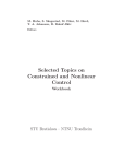
build up of gas. The slug cycle can be divided into four stages as shown by figure 2.1. It is
initiated by an accumulation of liquid in the low point of the pipe (stage 1). This will
eventually block the flow of gas and lead to a build up of pressure upstream the liquid slug.
The pressure and liquid slug will continue to grow (stage 2) until the pressure is high enough
to overcome the weight of the liquid in the riser. At this point the gas will start to penetrate
the liquid and push the slug all the way out of the riser (stage 3). This will result in a drop of
pressure and the gas will no longer be able to drag the liquid up the raiser. Some of the liquid
will therefore fall back down the riser(stage 4) and accumulate at the low point and initiate the
cycle again.
Figure 2.1
The slug flow cycle.
Theory
7
2.2 Flow through chokes
Knowledge about the behaviour of flow through chokes is important in production systems
where flow rates are controlled by choke valves. Different phases like gas, water and oil have
different flow behaviour through choke valves and other restrictions.
2.2.1 Single phase liquid flow through chokes
The flow rate through a valve depends on the size of the valve, the pressure drop over the
valve and the fluids properties according to the following equation [11].
Ql = C v z
∆Pv
ρ
(2-1)
Where:
Ql
Cv
Z
∆P
ρ
= Liquid flow rate
[l/min]
= Valve constant
= Valve opening [0 ≤ z ≤ 1]
= Pressure drop over the valve
= Density of fluid
2.2.2 Gas Flow through chokes
Gas flow through chokes is more complex then fluids because of its compressibility and
pressure temperature changes. Therefore corrections have to be made to the equation for
expansion and temperature. A correlation for the gas choke is given by [1].
(2-2)
Where:
qg,sc = Gas rate, standard conditions [Sm3 / s]
cd
= Discharge coefficient
A2
= Choke area [m2]
Z1
= Z-factor at choke inlet
T1
= Temperature at inlet [ºK]
ãg
= Specific gas gravity relative to air
p1
= Inlet pressure [Pa]
k
= Adiabatic gas constant
y
= Expansion ratio
Theory
8
2.2.3 Multiphase flow through choke
When two or more phases flow together in a pipe many different flow regimes may occur.
The different phases will also exhibit different behaviour when passing through a valve.
Correlations need to predict both critical and non-critical flow for all phases, and several
assumptions needs to be done.
Because of this complexity, valve sizing and characteristics are usually based on experimental
results.
2.3 Modelling
Storkaas [2] has developed a simplified dynamic model of multiphase flow for systems where
severe slugging occurs. The model covers both the stable limit cycle known as slug flow, and
even more importantly, the unstable but preferred stationary slug regime. This makes it
suitable for controller design. The model focuses on describing the observed macro-scale
behaviour rather then the detailed physics that governs the flow. For more details about the
model see Storkaas [2].
The macro-scale behaviour described by the model is:
• The stability of the solutions and the operational conditions as a function of choke
valve opening.
• The nature of the transition to instability.
• An unstable stationary solution at the same choke valve opening as those
corresponding to severe slugging.
• The amplitude/frequency of the oscillations.
Storkaas model is based on the following assumptions:
• Constant liquid level in the feed pipe, witch implies:
o Constant upstream gas volume.
• Only one liquid control volume.
• Two gas control volumes, separated by the low point, and connected through a
pressure-flow relationship.
• Ideal gas behaviour.
• Stationary pressure balance between riser and feed section.
• Simplified choke model for gas and liquid leaving the riser.
• Constant system temperature.
Theory
9
2.4 Controllability analysis
The following theory is found in [7].
2.4.1 Limitations imposed by RHP-zeros and unstable poles.
.
A linear dynamic system can be represented as x = Ax + Bu . The system is stable if and only
if all the poles are in the left half plane(LHP), Re{i ( A)} p 0 ∀ i.
Unstable poles can be stabilized by feed back control. Right half plane (RHP)-poles impose a
lower bound on the bandwidth wc for a system. [7] provides the following lower bound for
RHP poles.
Wc f 2 p
(2-3)
and for imaginary poles
Wc f 1.15 | p |
(2-4)
RHP-zeros results in an inverse response and impose an upper bound on the bandwidth for
any system using feedback control. When a system is using feedback control the closed loop
poles will approach the open loop poles as the gain approches infinity. This makes the system
unstable and limits the bandwidth for high gains. The bound on the upper bandwidth for a
system with real RHP-zeros is
Wb ≈ Wc p
zn
2
(2-5)
And for complex zeros
⎧| z n | / 4 Re( z ) >> Im( z )
⎪
Wb ≈ Wc p ⎨| z n | / 2.8 Re( z ) = Im( z )
⎪| z |
Re( z ) << Im( z )
⎩ n
(2-6)
RHP-zeros close to the origin of coordinates impose the largest constraints on the bandwidth.
Control is more difficult if the zeros are located close to the origin of coordinates compared to
zeros close to the imaginary axis. When both RHP-poles and zeros are present in the same
system, the given upper and lower bounds on the bandwidth will make the stabilizing of the
system impossible.
In order to fulfil the limitations imposed on the bandwidth and achieve a satisfactory
performance and resilience the following is demanded
Zn > 2.4|p|
(2-7)
Experimental testing and verification
10
3 Experimental testing and verification
3.1 Apparatus
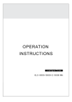
Figure 3.1 shows an overview of the lab-scale Miniloop that was used during the
experimental face of this thesis. The Miniloop was originally constructed by Bårdsen [3] as a
part of his fifth grade project with the Department of Chemical Engineering at NTNU. Some
changes have been made to the original Miniloop, including purchase and installation of
additional equipment. These changes will be addressed later on in this chapter.
Figure 3.1
Flow sheet for the Miniloop.
As can be seen from the figure the Miniloop has a water (WT) and an air source. The water is
pumped from the reservoir into the system, while the air is let into the system from a
pressurized air outlet in the wall. The flow rate of water and air is controlled by manually
adjusting valves V1 and V2. The pipeline system is constructed of several connecting sections
of transparent plastic tubes. The pipeline is meant to imitate the pipeline topography where
gravity induced slugging occurs, which is a low point connected to an inclined section of the
pipe. At the top of the riser the multiphase flow passes the control valve before it enters the
separator. At this point the air is released out of the system through an open hole in the
separator, while the water is returned to the reservoir. To monitor the behaviour of the system
a combination of pressure measurements and slug sensors are used. As can be seen from
Figure 3.1 the water has a blue colour. This is a necessity and not a just a cosmetic issue. The
reason is that the slug sensors are optical in nature and the water had to be a colour that
allowed it to absorb the light emitted from the sensors. This will be addressed more
thoroughly in chapter 3.4.1.
Experimental testing and verification
11
3.1.1 Equipment
Table 3.1 lists the different equipment used in the Miniloop. Consult table A.1 in the user
manual appended to this thesis for more info about the distributors and prises. More detailed
information about the different equipment can be found in the user manual, appendix B.
Table 3.1List of equipment.
Notation
FT.W
FT.A
P1
P2
P3
S1
S2
PU
WT
BT
ST
CV
Equipment
Rate meter for water(Gemu 3021)
Rate meter for Air
Pressure sensor (MPX5100DP) Feed inlet
Pressure sensor (MPX5100DP) Valve
Pressure sensor (MPX5100DP) Separator air outlet
Slug sensor (E3X-DA-N)
Slug sensor (E3X-DA-N)
Pump (Eheim 1060)
Reservoir
Buffer tank
Separator
Control valve
The rate meter for water (Figure 3.2) is
placed in front of the mixing point of water
and air. The digital display shows the rate
of water in l/min. It provides a signal
between 4-20mA, depending on the rate of
flow, which is send to the computer.
Figure 3.2
Rate meter for water
Figure 3.3
Rate meter for air
The rate meter for air (Figure 3.3) is placed
in front of the mixing point of water and air.
It has a digital display that shows the rate of
air in percent of its operating area, witch is
0-2.2 l/min. The rate meter also provides a signal
between 0-5 V which is send to the computer.
Experimental testing and verification
The pressure sensors (Figure 3.4) is one of
Motorola’s differential pressure sensors that
delivers a signal between 0.2-4.5 V. The
relationship between voltage and pressure is
linear and its operating area is between
0-100kPa.
Figure 3.4
Pressure sensor
Figure 3.5
Slug sensor
Figure 3.6
Pump
The slug sensors (Figure 3.5) are fibre
optical sensors. Each slug sensor is made up of
two fibre optical cables connected to a sensor.
The light emitted from the senor will
travel out through one of the cables and back
through the other. The device will provide a
signal between 1-5 V depending on how much
light is transmitted between the two cables.
The pump used is a standard aquarium pump.
It can deliver up to 38 l/min and work against
a head of 3.1 m. Special care must be taken to
make sure it doesn’t pump air as this can
damage the pump.
12
Experimental testing and verification
The reservoir (Figure 3.7) is a cylindrical
container made of transparent glass. It serves
as the water source for the Miniloop, and
the water is returned to the tank from the
separator.
Figure 3.7
Reservoir
Figure 3.8
Buffer tank
Figure 3.9
Separator
The buffer tank (Figure 3.8) is a cylindrical
container made of transparent glass.
For slugs to appear the system needs a
sufficiently large air volume. The air volume
in the tank can be altered by adding water to
the tank.
The separator is also a cylindrical
glass container with one inlet and two
outlets. The air is released to the surroundings
through an open hole in the top, while the
water is returned to the reservoir.
13
Experimental testing and verification
14
The control valve is located at the top of
the riser before the separator inlet. The
valve requires a 24V power supply and
is controlled by a signal to the actuator
between 4-20 mA. The relationship
between the valve’s actuator an the valve
opening is linear. To operate the actuator
an external pressurized air source of 4-8
bar is required to counteract the spring power.
The lab has its own pressurized air source,
which was used for this purpose.
Figure 3.10
Control Valve
3.1.2 Changes to the Miniloop
As mentioned above some changes have been made to the Miniloop since it was constructed
by Bårdsen. These changes include modification of existing equipment and purchase of new
parts.
In the original loop permanganate was used to dye the water red. The Miniloop had been out
of use for some months, so the colouring matter used had stained the pipes. These stains
created problems for the optical sensors. For reasons that will be made obvious in chapter
3.4.1 all the tubes were replaced and a more water-soluble colouring matter was added. The
new colouring matter added is called Vulcanosol-Blau 684.
The original brackets used to attach the slug sensors to the pipe had a couple of flaws. In the
original bracket there was no way to adjust the distance between the two optical cables. There
was also some concern that the metal used in the brackets could reflect some of the light and
create an error in the measurement. After some consideration a new design was chosen.
The new bracket (figure 3.5) was drilled out of a PVC pipe to resemble a horseshoe. With this
design the distance between the two cables could be altered depending on how far into the
material the cables were screwed.
One of the biggest problems with the original loop was that we had no way of ensuring the
same operating conditions each time an experiment was conducted. There was a flow meter
installed to measure the flow of water, but we lacked a way to measure the flow of air. For
this reason a flow meter for air was purchased and installed. An additional pressure sensor
was also installed at the air outlet of the separator. The purpose of this sensor was to estimate
the air flow through the control valve.
Experimental testing and verification
15
3.2 Data Flow and Data logging
The data measured by the devices installed on the Miniloop had to be recorded, analyzed and
stored. To accomplish this, the different devices are connected to a lap top computer through
the Field Point modules (Figure 3.11). The Field Point modules are mounted on a terminal
base inside a water proof locker. The different analogue transducers are connected to the FP
input module (middle), while the control valve is connected to the FP output module (right).
The computer is connected to the communication module to the left.
Figure 3.11
Picture of the FP modules mounted on the termination card.
3.2.1 Software and drivers
The hardware (FP modules) and software required to analyze, store and display the data are
delivered by National Instruments (NI).
The software needed is LabView with the following additional content installed :
• PID control toolset.
• Fieldpoint explorer version 3.01 drivers ( FP module drivers)
Experimental testing and verification
16
3.3 LabView
“LabVIEW delivers a powerful graphical development environment for signal
acquisition, measurement analysis, and data presentation, giving the flexibility of a
programming language without the complexity of traditional development tools.”[12]
The user interface in LabVIEW is called a Virtual Instrument (VI). These VI’s have to be
made for the specific measuring set-up, in this case for the Mini-Loop. The programming
language used in LabVIEW is called G, and is a graphical drag-and-drop programming. This
programming language is based on C+, and LabVIEW supports additional code both in C+,
Visual Basic and Matlab Scripts.
LabView consists of three main parts. The front panel is the interactive user interface of a VI,
so named because it simulates the panel of a physical instrument. The front panel can contain
knobs, push buttons, graphs and many other controls (user inputs) and indicators (program
outputs). Data or control can be input by a mouse or a keyboard, and results can be viewed
by the program on the screen.
LabVIEW includes a wide array of visualization
features, including tools for charting and graphing. This
makes it easy to visualize data. The user simple drags
and drops the desired controls or indicators from the
build-in control palette to the front panel.
Figure 3.12
Labview Front Panel.
The second part of LabVIEW is the block diagram. Its in the block diagram that the data is
acquired, analyzed and generated. While the front panel is the user interface, the block
diagram is the VI's source code. It is constructed in LabVIEW's graphical programming
language, G. The block diagram is the actual executable program. The components of a block
diagram are lower-level VIs, built-in functions, constants, and program execution control
structures. You draw wires to connect the appropriate objects together to indicate the flow of
data between them. Front panel objects have corresponding terminals on the block diagram so
that data can pass from the user to the program and back to the user.
The hierarchy window displays a graphical representation of the calling hierarchy for all VIs
in memory, including type definitions and global variables. This hierarchy window shows the
relationship between the subVIs in a program. This is a good insight to the structure of the
program. The power of G programming lies in the hierarchical nature of VIs. After creating
a VI, one can use it as a subVI in the block diagram of a higher level VI.
Experimental testing and verification
17
3.3.1 Miniloop front panel
Figure 3.13 shows the front panel for the LabVIEW program miniloop. The original program
created by Bårdsen [3] were abandoned, and a new one was created from scratch to
accommodate better flexibility and different control structures. The front panel serves as the
interface between the user and the lab scale Miniloop.
Figure 3.13
The front panel for the labview program miniloop.
The front panel has three main areas of interest. First you have the charts used to visualize the
measurements, like pressure drop, valve opening, flow and hold up. The top chart displays the
downstream pressure, while the second one displays the upstream pressure. If anti slug
control is applied the mentioned charts will display the relevant set point. The third chart from
the top plots the flow of water into the system and an estimate of the flow through the control
valve. If a cascade controller is applied it will also show the relevant set point. The slug
sensor results are plotted at the bottom. This measurement plots the filtered signal received
from the optical sensors.
The PID control is located at the lower left corner of the screen. This is were the user chooses
witch control structure to use. The loop is set to “no control” by default, but by clicking it you
can choose the following control structures from the pull down menu:
• No control.
• PI control, with P1 as the controlled variable.
• Cascade control, with mass flow (W) as the main variable and P1 in outer loop
• Cascade control, with mass flow (W) as the main variable and P2 in outer loop.
18
Experimental testing and verification
The tuning parameters for the different controllers are also located here, witch means the user
can change them by simply entering the new value.
In the upper left corner of the front panel the user will find some additional indicators that
displays additional information about the system. These include density, actuator position and
digital displays for the flow. When the system is running in open loop mode, “no control”, the
valve opening can be set through the slide bar. Most measurements are already filtered to
some degree, but since the estimated flow measurement is the one most prone to disturbances,
an additional lag filter has been added. The parameters for this filter can be altered by
changing the values in the filter box.
When the program is shut down it is recommended to use the big red stop button located on
the front panel to ensure a controlled termination of the program, including the writing of data
from memory to hard drive. The data will be stored in a text file with the following format
Table 3.2
Format of stored data.
t [msek]
S [V]
P1 [Barg]
P2 [Barg]
…
…
…
…
…
…
…
…
Qinlet
[l/min]
…
…
Westimated
[kg/min]
…
…
Z [-]
…
…
All kinds of data can be written to the file, including other measurement, calculations etc.
Adding another source of data to the stored file is a simple matter. All the user has to do is
connect the measurement to be stored to a subVi in the block diagram. Consult the user
manual in appendix B to learn how.
Experimental testing and verification
19
3.3.2 Miniloop block diagram.
As mentioned the block diagram contains the source code for the program. The diagram is too
large to be displayed in its entirety, but figure 3.14 shows a simplified sketch of the dataflow
inside the block diagram. A while loop encompass most of the program code.
The field point modules will provide the while loop with the data sampled from the
measurement devices. Inside the loop the data is calibrated, filtered and modified to provide
the measurement needed for control purposes. The box labelled “control structure” is a case
structure that contains the different control structures mentioned in chapter 3.3.1. The code
inside the while loop will provide the control structure with the measurements needed, and the
actuator position will be send back to the field point modules through the while loop. If no
control is active, the control structure will return the actuator position set by the sliding bar in
the front panel.
Figure 3.14
The data flow inside the block diagram.
Figure 3.15 shows about 1/4 of the block diagram associated with the miniloop program. To
view the diagram in its entirety the reader should open the miniloop program on a computer
with Labview installed and access the block diagram (ctrl+e). The program can be found on
the cd that accompanied this thesis. The partial frame seen in the lower right corner is the
control structure in figure 3.14.
Experimental testing and verification
Figure 3.15
20
Section of the block diagram.
To make the programming environment in LabVIEW less messy, much of the code is
grouped together to create different sub Vi`s. Figure 3.16 shows the content of the sub VI
called “Calibrate”. In this sub Vi the different measurements are calibrated and converted
from mA and V signals to engineering units. The hierarchy window (figure 3.17) shows the
relationship between the different subVIs in the program.
Experimental testing and verification
Figure 3.16
The content of the sub VI named “calibrate”.
Figure 3.17
Section of the hierarchy window.
21
Experimental testing and verification
22
3.4 Data analyzing and filtering
Previous work on the Miniloop by Bårdsen included the implementation of a simple PI
controller to stabilize the process. This controller used the downstream pressure (P1) as the
controlling variable. This measurement however can be hard to obtain in practical problems
like offshore installations. One of the goals of this thesis was therefore to expand the work
done by bårdsen[3] by implementing a cascade controller. Previous work by Storkaas[4]
suggested that a cascade controller using mass flow(W) or volume flow(Q) as the controlled
variable could stabilize the process. A measurement of the mass or volume flow would have
to be estimated from other available measurements like the slug sensor. Before such an
estimate could be obtained the slug sensor had to be analyzed further.
3.4.1 Slug sensors
The slug sensors had been installed by Bårdsen when the loop was build, but no work had
been done on analyzing the signals they produced. The original signals (figure 3.18) consisted
mainly of a constant signal interrupted with spikes. The purpose of the slug sensors was to
measure the hold-up, and it soon became apparent that the signals had to be treated further if
any useful information were to be gained from them.
Figure 3.18
Initial readings from the slug sensors.
As mentioned earlier the slug sensors are based on fibre optical technology. Two separate
optical cables are connected to a sensor. Light is emitted from the sensor and travels through
one of the cables. As the light exits the first cable it will travel through the medium to be
measured. The second cable is mounted on the other side of the medium, directly opposite the
first cable. The light emitted from the first cable travels through the medium, and is returned
to the sensor through the second cable. The sensor will produce a signal between 1 and 5 volts
depending on the amount of light that returns. A signal of 1 volt means that no light has
returned to the sensor, while 5 volts means all the light has returned.
The original range of application of the optical sensors is as a precision sensing device. The
precise location of an object could be determined because the object would block part of the
light beam, hence reducing the amount of light transferred between the cables. As long as
only air was present in the pipe all the light would pass through the pipe and return to the
sensor via the second cable. The goal was to estimate the hold up of liquid by measuring the
amount of light absorbed by the liquid phase. Since the sensor was intended to be used on
solid objects this turned out to be a big challenge.
As can be seen from figure 3.18 the optical sensors delivered a constant signal of 5 volt
independent of whether it was liquid or air in the pipe. After further experimentation it was
Experimental testing and verification
23
discovered that the spiked were caused by a phase transition between air and liquid and vice
versa. When the light hit such a transition the angle of the liquid surface would deflect the
light away, resulting in the spikes witch indicated that no light returned to the sensor.
This still did not explain why the sensors showed the same value for both water and air. There
were some speculations that the water didn’t absorb enough light for the sensor to measure a
difference. The solution proved to be as obvious as it was simple. The colouring matter used
in the liquid was permanganate. This gives the liquid a red colour. However, the property of a
red substance is that it will absorb all light from the colour spectrum except red. By taking the
fact that the optical sensor used red light as its source into consideration, the solution was
obvious. The water in the loop was changed and a blue colouring matter was added.
This gave the desired response on the sensors as can be seen from figure 3.19.
Figure 3.19
The slug sensor after the colouring matter was changed.
By adding more colouring matter, the amount of light absorbed by the liquid would increase,
and the lower value corresponding to pure liquid was reduced from 3 Volt to 2 volt. The
sensors digital display showed a value ranging from 0-4000, corresponding to 1-5 V, where
the value 1500 represented pure liquid. The lower boundary for the sensor output was
changed to 1700, making 1700 (pure water) correspond to 1 V and 4000 (pure air) to 5V. In
effect this cuts off all values below 1700, including most of the spikes (figure 3.20).
Figure 3.20
The slug sensor after signal scaling.
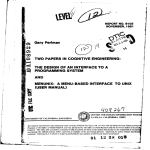
The slug sensor now gives a lot of information about the slug cycle. From figure 3.20 a value
of 5 indicates that there is only air in the pipe. A slug is building up in the raiser, and when
the downstream pressure gets high enough it will push the slug up through the raiser. This can
be seen when the value drops from 5 to 1 volt. The air will eventually penetrate the liquid
witch is represented by the oscillations between 1 and 5 volts. The liquid then falls back to the
low point, causing the value to increase to 5 again before the cycle repeats itself.
Experimental testing and verification
24
The nature of the slug flow creates some restrictions and limitations witch reduces the
effectiveness and accuracy of the slug sensor. In normal gravity induced slugging the gas
would penetrate the liquid as bubbles in the liquid flow. This would allow the optical sensor
to estimate the fraction of water passing the sensor giving us the hold up.**
However, conditions in the raiser produced a flow regime during closed loop where large
volume of gas flowed as a separate phase in-between the liquid bulks (figure 3.21).
Figure 3.21
Slug flow pattern in the pipe
The slug sensor will therefore only be able to indicate the presence of water or air, not a mix
of both. The oscillations (figure 3.20) are therefore a result of this flow pattern and the
disturbances caused by the phase transitions. By adding a frequency filter in LabVIEW, the
measurement was improved further (figure 3.22) by removing some of the disturbance and
averaging the data.
Figure 3.22
Final slug sensor readings.
To transform the volt signal in figure 3.22 to a hold-up measurement, some algebraic code
were added to Labview. These take into account the geometry of the tube and scale the hold
up to take values between 0 and 1.
** Had this been the case the slug sensor would probably not have been useable. The surface
of the bubbles would have deflected the light away from the optical sensor, resulting in severe
disturbances.
25
Experimental testing and verification
3.4.2 Estimating the flow through the choke valve
The mass and volume flow through the choke valve can be estimated by measuring the
pressure drop over the choke and the mixture density. Multiphase flow through a choke valve
is complex, but according to Skogestad there have been successful implementations of a
cascade controller in the industry by using a simple valve equation for liquid flow. An attempt
was therefore made to estimate the flow from equation 2-1.
The mixture density could be estimated from the hold up measurement, xl, by the following
equation :
ρ m = xl ⋅ ρ water + (1 − xl ) ⋅ ρ air
(3-1)
The biggest challenge lay in experimentally deciding the valve characteristics.
The only available measurements were the flow rates into the system. The slugging nature of
the system also made it impossible to get any experimental stationary open loop values when
using both gas and liquid. For that reason it was decided that the only viable option was to
decide the valve characteristics using only liquid flow. When only water was pumped through
the system, a simple conservation consideration meant that the flow meter at the inlet would
show the liquid flow through the valve. Water was pumped through the system, the actuator
position was altered, and the corresponding pressure drop over the choke valve and liquid
flow into the system were recorded. For pure liquid flow the density in equation 2-1 could be
dropped since ρ m =1.
Pressure drop [barg]
2.5
2
1.5
1
0.5
0
0
10
20
30
40
50
60
valve opening %
70
80
90
100
0
10
20
30
40
50
60
Valve opening %
70
80
90
100
Liquid flow rate [l/min]
0.2
0.15
0.1
0.05
0
Figure 3.23
Pressure and flow vs. valve opening
26
Experimental testing and verification
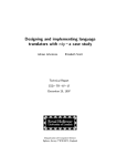
As can be seen from figure 3.23 valve openings above 30% seems to have little or no effect
on the pressure or flow rate. This suggested that the valve were oversized. If equation 2-1
were to be valid the relationship between Q and z ∆P had to linear. However as can be seen
from figure 3.24 this was not the case.
2.5
2.4
2.3
Q [l/min]
2.2
2.1
2
1.9
1.8
0.002
0.004
0.006
0.008
Figure 3.24
0.01
z*SQRT(dP)
0.012
0.014
0.016
0.018
Q vs Z*SQRT( ∆P )
In an attempt to determine the valve characteristics two different approaches were tested.
The first was to try and fit the experimental data to equation 3-2 by a linear parameter
estimation(method a), and the second was to estimate f(z) from equation 3-3 by plotting
Q/ ∆P against z(method b). Both methods are described in more detail in appendix A.4.
Q = k ⋅ z n ∆P
(3-2)
Q = f ( z ) ∆P
(3-3)
Both methods proved unsuccessful when trying to fit it to the entire data range. In order to get
an estimate of the flow a purely mathematical approach had to be abandoned. For control
purposes the priority had to be to obtain a satisfactory flow estimate in the area with small
valve openings. As mentioned earlier valve openings above 30% seemed to have little or no
effect on the flow rate. The two approaches mentioned above were therefore attempted on the
data set below 30% valve opening. The best results were obtained by method b when a fifth
order polynomial was used to describe f(z).
27
Experimental testing and verification
20
Datapoints
18
Poly. (Datapoints)
16
Q/sqrt(dP)
14
12
10
8
6
4
2
0
0
0,05
0,1
0,15
0,2
0,25
0,3
0,35
Valve position [z]
Figure 3.25
Fitting the f(z) to the datapoints.
The fifth order polynomial fitted to the data using the least squares method is
f (z ) = 70223z 5 − 61350 z 4 + 19191z 3 − 2705.4 z 2 + 229.44 z
(3-4)
Combined with equation 3-3 this estimated the flow through the valve for valve openings
below 30%. To make the equation valid for valve positions above 30% a linear relationship
were assumed between the flow rate and the pressure drop by setting f(z)=f(0.3) for all valve
openings above 30%.
⎧ f ( z ) ⋅ ∆P for 0 ≤ 0.3
Q=⎨
⎩ f (0.3) ⋅ ∆P for z f 0.3
(3-5)
Estimating the volume liquid flow through the choke was now possible. Unfortunately it
proved impossible to get an estimate of the volume gas flow through the choke with the
current measurement setup. This in turn made it impossible to estimate the total volume flow
Q. The total mass flow W was still a viable option though. The mass flow of gas was assumed
to be much smaller then the mass flow of the liquid. So setting the total mass flow W equal to
the mass flow of liquid would not introduce to big an error. A simple rearrangement of
equation 3-5 would therefore give an estimate of the total mass flow.
Experimental testing and verification
⎧⎪ f ( z ) ⋅ ∆P ⋅ ρ m for 0 ≤ 0.3
W = n⋅⎨
⎪⎩ f (0.3) ⋅ ∆P ⋅ ρ m for z f 0.3
28
(3-6)
Where n is a tuning parameter set to 1.3.
The system was forced into steady state by using active control. A simple mass balance
consideration now implied that the total mass flow through the choke had to be the same as
the mass flow into the system. The parameter n could then by tuned so that the estimated mass
flow W would be the same as the measured liquid flow into the system.
Figure 3.26
Snapshot of the chart showing displaying the measured mass flow.
Figure 3.26 shows a snapshot of the flow chart on the miniloop front panel. The red line is the
measured flow into the system while the white line represents the estimated mass flow
through the top side choke. The left side of the chart displays the Miniloop in open loop
mode, while active control is used on the right side. The estimate of the mass flow could now
be used for control purposes.
29
Experimental testing and verification
3.5 Open loop experimental data
The Miniloop was run in open loop and the valve opening was gradually changed from fully
open till fully closed. The corresponding pressure drops were recorded and analyzed to create
the bifurcation diagram(figure 3.27).
0.25
Maks trykk
Min. Trykk
P 1 [barg]
0.2
0.15
0.1
0.05
0
10
20
30
40
0
10
20
30
40
50
60
70
80
90
100
60
70
80
90
100
0.08
P 2 [barg]
0.06
0.04
0.02
0
-0.02
Figure 3.27
50
VentilÅpning %
Bifurcation diagram for the experimental data.
As can be seen from figure 3.27 the system is stable up to a choke opening of 19 %. If the
choke is opened further the system will enter the slug flow regime. The system becomes
unstable and the pressure will start to oscillate. Early solutions to the slug problem in the oil
industry utilized this property. By increasing the pressure drop over the top side production
choke the slugging was successfully eliminated. However this solution also increased the total
pressure drop in the well-pipeline system, resulting in lower oil recovery.
3.6 The simplified slug model
The model used to describe the riser slugging behaviour is not a partial differential equation
system, but a simplified bulk model. The model has only three states, the mass of gas behind
the slug, the mass of liquid in the slug and the mass of the gas in front of the slug. Riser
slugging as described by the simplified model can be seen in figure 3.28.
30
Experimental testing and verification
Figure 3.28
Model characteristics with important parameters.
The model was tuned to fit the experimental data as shown in figure 3.29. The red lines is the
data from the simplified slug model while the blue dotted lines shows the experimental dataThe red dashed line indicates the presence of an unstable stationary solution at the same
choke valve openings as those corresponding to severe slugging.
0.25
Storkaas simplified model
experimental data
P1 [barg]
0.2
0.15
0.1
0.05
0
0.1
0.2
0.3
0.4
0.5
0.6
valve opening(z) [-]
0.7
0.8
0.9
1
0
0.1
0.2
0.3
0.4
0.5
0.6
Valve opening(z) [-]
0.7
0.8
0.9
1
0.08
P2 [barg]
0.06
0.04
0.02
0
-0.02
Figure 3.29
Bifurcation diagram for the simplfied slug modell.
Experimental testing and verification
31
It is unrealistic to achieve a good fit for both the slug regime and the stationary regime for the
entire range of valve openings, so some priorities had to be made during the tuning of the
model.
If the controller is to work properly the actuator has to have a significant impact on the
process. For the high range valve openings, the pressure drop over the choke is too small for
the effect of a small change in valve opening to be significant. This means that the only area
of interest is that from medium to small valve openings. This can be seen from the bifurcation
diagram because it shows little to no variations from medium to high valve openings.
Secondly, the unstable, stationary regime is more important then the stable oscillatory
regime. The reason for this is that the goal is to achieve stationary flow with active control in
the unstable area. By avoiding the slug regime and operating at the stationary regime, the
focus is on where you want the process to be and not where you don’t want it to be.
A good example of this was presented by Storkaas in [2].
“If you are teaching someone to ride a bike, you are teaching
them how the bike behaves when they have mastered the
balancing act(the desired unstable operating point),
not how it behaves when it lies on the ground (the undesired slug flow)”
When taking these priorities into consideration the simplified model shows a good fit to the
experimental data. The model fit to the experimental data for the upstream pressure (P1), is
actually very good for the entire valve opening range. The fit for the downstream pressure is
acceptable for the low to medium valve openings. The deviations in amplitude for higher
valve openings are acceptable in light of the priorities given.
Part of the deviations for the downstream pressure fit may result from the disturbances
associated with the downstream measurement. The downstream measurement is also located
15 cm below the valve, witch will cause the experimentally measured pressure drop to be a bit
higher then it should. By examining the bifurcation diagram it can be seen that the
experimental pressure drop over the choke is oscillating to a lesser degree in the stable
regime. The mayor cause for this behaviour is caused by the flow behaviour as described by
figure 3.21.
The frequencies of the oscillations are not included in the bifurcation diagram. Figure 3.30
and 3.31 shows the open loop behaviour for a valve opening of 30% for both the model and
the lab scale Miniloop. The amplitude of oscillations for the upstream pressure P1 are almost
the same for both the model and the Miniloop. The model calculates a bit lower amplitudes
for the downstream pressure P2. By examining the frequency of oscillations it can be seen
that the slug frequency is about 10% higher for the Miniloop compared to the simplified
model. In this case the model was tuned to achieve a good fit for the amplitude. Since the
upstream gas volume is fixed in the model it was impossible to fit both amplitude and
frequency.
32
Experimental testing and verification
0.16
P1 [barg]
0.14
0.12
0.1
0.08
0.06
0
0.2
0.4
0.6
0.8
1
time [min]
1.2
1.4
1.6
1.8
2
0
0.2
0.4
0.6
0.8
1
time [min]
1.2
1.4
1.6
1.8
2
0.04
P2 [barg]
0.03
0.02
0.01
0
Figure 3.30
Open loop behavior for the miniloop (z=0.3)
0.16
P1 [barg]
0.14
0.12
0.1
0.08
0.06
0
0.2
0.4
0.6
0.8
1
time [min]
1.2
1.4
1.6
1.8
2
0
0.2
0.4
0.6
0.8
1
time [min]
1.2
1.4
1.6
1.8
2
0.04
P2 [barg]
0.03
0.02
0.01
0
Figure 3.31
Open loop behaviour for the simplified model (z=0.3)
33
Experimental testing and verification
3.7 Controllability analysis
This analysis is based on a linearized model around a typical unstable operating point. The
operating point chosen is z=0.3. The system is unstable for this valve opening in open loop
since there is a complex pair of poles in the RHP (table 3.3). To compare it with an operating
point that should be in the stable area according to the bifurcation diagram the poles for
z=0.15 are also included in the table. As can be seen these poles are in the LHP, hence
making the system stable. The poles and zeros for other operating points can be found in
appendix A.3. The real part of the worst pole has been evaluated and plotted against the valve
opening in figure. The poles start in the LHP and move over to the RHP when the valve
opening is z=0.19. This corresponds with the bifurcation diagram where the system is
unstable for z ≥ 0.19.
RHP poler gives a lower limit on the bandwidth for the process. This means that the lower
limit for the bandwidth will increase as the valve opening increases. The system can be
stabilized by using feedback control to move the poles. RHP-zeros results in inverse response
and imposes an upper limit on the bandwidth for the process. To obtain stability with a
satisfactory performance the following is required
WC > 1.15|p| zn > 2.3|p|
Table 3.3
(3.6)
System poles
Valve opening
z=0.15
z= 0.3
λ1
-9.5311
-10.4951
λ2
-0.0133 - 0.1862i
0.0522 - 0.3265i
λ3
-0.0133 + 0.1862i
0.0522 + 0.3265i
RHP-pole length
0.1867
0.3306
The different measurements available are listed below.
Table 3.4 Available measurements.
Measurement
P1
P2
ρm
W
Q
Unit
[bar]
[bar]
[Kg/m3]
[Kg/min]
[l/min]
Description
Upstream pressure(feed inlet)
Downstream pressure
Density
Total mass flow
Total volume flow
The only upstream (downside) measurement is the pressure P1. All the other measurements
are upstream (topside) measurements. The zeros for the different measurements are given in
table 3.3.
Table 3.5 Zeros for the different measurements at the operating point z=0.3.
P1
-0.1673
P2
0.8720 + 0.6347i
0.8720 - 0.6347i
ρm
0.0958
0.0226
W
-13.027
-0.0092 + 0.0614i
-0.0092 - 0.0614i
Q
-5.6430
-0.1530
-0.0401
34
Experimental testing and verification
The upstream pressure P1 has one LHP-zero. Since LHP-zeros imposes no fundamental
control problems P1 would be the obvious choice of measurement. However, this
measurement can in many cases be either unreliable or unavailable and other measurements
have to be considered. From the bandwidth limitations imposed by equation 3.6 there cant be
any RHP-zeros smaller then 0.7605. Of the alternatives in table 3.3 ρm have RHP-zeros close
to the unstable poles. This makes it unsuitable as a measurement for a stabilizing controller
due to the bandwidth limitations imposed. From table A.2 it can be seen that the zeros for P2
increases as the valve opening increases. At the operating point of z=0.3 it is larger then
0.7605 and cant be directly dismissed as a possible measurement. The model in [4] gets lower
zeros for P2 conludes that it cant be used for a stabilizing controller. Both Volume flow Q and
mass flow W appears to be better alternatives, but they both have LHP-zeros close to or at the
imaginary axis. An attempt to stabilize the system with one of these measurements would
result in an almost integrating closed loop system. According to Storkaas a cascade control
could solve this problem by using a combination of a flow measurement and some other
measurement, e.g pressure.
0.6
0.5
Real part of the worst pole
0.4
0.3
0.2
0.1
0
-0.1
0.1
Figure 3.32
0.2
0.3
0.4
Real part of the worst pole.
0.5
0.6
valve opening, z [-]
0.7
0.8
0.9
1
35
Experimental testing and verification
3.8 Anti slug control
In this chapter different control structures will be tested on the Miniloop, and they will be
compared to simulations performed on the simplified slug model. The criteria for satisfactory
control is to stabilize the system at a valve opening that would normally result in severe
slugging in open loop.
3.8.1 Control with upstream measurements
According to the controllability analysis the best choice of measurement would be the
upstream pressure P1. A simple PI controller with gain K=22 bar-1 and integral time Ti=10s
will stabilize the system as shown in figure 3.33. The system starts from a state of severe
slugging, and the controller is turned on after two minutes. After an additional two minutes
the controller is set to manual and the slugging reappears. The top chart in figure 3.33 shows
the upstream pressure P1 vs. time. The blue line is the pressure and the red line is the set point
for the pressure controller, witch was set to 0.115 barg. The controller stabilizes the system
quickly if a bit aggressive. The stabilized system experiences small pressure oscillations,
however these are small compared to the amplitude of the slugging, so the tracking
performance of the controller is considered as good. The actuator use is acceptable. It’s
constantly making small adjustments to keep the system stable and at the stationary unstable
solution. It is evident that the system is stabilized in the unstable region since the valve is
operating at a valve opening that lies in the unstable are for open loop. This can be seen from
the bifurcation diagram (figure 3.29). As excepted the slugging reappears quickly after the
controller is turned off. In light of the control objective the pressure controller is performing
very well.
0.16
Pressure P1
Setpoint
P1 [barg]
0.14
0.12
0.1
0.08
0.06
0
1
2
3
time [min]
4
5
6
0
1
2
3
time [min]
4
5
6
1
Valve postition [-]
0.8
0.6
0.4
0.2
0
Figure 3.33
Performance of a pressure controller on the miniloop.
Experimental testing and verification
36
A simulation was also run on the simplified slug model (figure 3.34) using the same
parameters for the gain and integral action as above. The set point for the controller was also
the same (0.115 barg). As above the pressure is represented with the blue line and the red line
indicates the set point. The simulation starts in open loop resulting in severe slugging. After 2
minutes the controller is turned on. After an additional 3 minutes the controller is returned to
manual mode. The controller quickly stabilizes the system and the tracking performance is
very good. The actuator use is minimal as it moves towards the valve opening corresponding
to the set point of 0.115 barg. It seems to stay stable at this value, however if one had zoomed
in on the graph one would have seen that the actuator is continuously making small
corrections to hold the system stable.
Figure 3.34
Performance of a pressure controller on the simplified model.
By comparing the simulation to the experimental data(figure 3.33) it is obvious that the
simplified model is in accordance with the experimental data.
The simplified model simulates the results obtained experimentally very accurately. More
importantly, the controller in the simulation reproduced the stability results obtained
experimentally from the lab scale Miniloop. The biggest difference between the model and
the Miniloop is the time it takes for severe slugging to reappear after the controller is turned
off. While this takes less then a minute for the Miniloop, the model requires almost three
minutes. The reason for this is that the simplified model contains little noise causing the
pressure to stay close to the reference value for a longer time.
Experimental testing and verification
37
3.8.2 Control with downstream measurements
In the previous chapter it was shown that a simple PI controller could stabilize the system
using one upstream measurement (P1). As mentioned earlier this measurement is in many
cases not even installed. In other cases it will often prove unreliable or unusable for control.
The controllability analysis in chapter 3.7 provided the basis for exploring other possibilities.
P2 as measurement.
The controllability analysis could not dismiss the pressure drop as possible measurement. For
this reason an attempt was made to stabilize the Miniloop by using a pressure controller with
P2 as the measurement. All attempts to stabilize the system proved unsuccessful and P2 was
dismissed as a possible measurement for a stabilizing controller. Since the controllability
analysis in [4] had excluded P2 as a measurement it will not be treated any further here.
3.8.3 Cascade control
According to the controllability analysis both the total mass flow W and total volume flow Q
were better suited for a stabilizing controller. However stabilizing the system with one of
these measurements would lead to an (almost) integrating closed loop system, but a cascade
configuration with a pressure measurement in the outer loop could solve this problem.
Because of the problems with obtaining an estimate of the volume flow rate (chapter 3.4.2)
the mass flow W was chosen as the measurement. Two different cascade configurations were
tested where the downstream- and upstream pressure were used for feedback purposes.
38
Experimental testing and verification
3.8.4 Mass flow W and upstream pressure P1
Figure 3.35 shows that a cascade controller using mass flow W in the inner loop and upstream
pressure P1 in the outer loop will stabilize the system. The system is started in open loop with
severe slugging and the controller is turned on after 2 minutes. After an additional 3.2 minutes
the controller is switched back to manual. The inner loop uses a pure proportional controller
while the outer loop uses both proportional and integral action. The parameters for the gain
and integral action are listed in table 3.6.
Table 3.6 Tuning parameters
K
Ti
Inner loop
0.8 [bar-1]
-
Outer loop
15 [min/kg]
30 [s]
The two upper charts show the pressure vs. time and the mass flow vs. time. The red line
indicates when the controller is active and represents the set point of 0.115 barg for the outer
loop. The set point for the inner loop is provided by the outer loop. The actuator use is
displayed in the bottom chart.
0.16
P1
Setpoint
P1 [barg]
0.14
0.12
0.1
0.08
0.06
0
1
2
3
4
5
time [min]
6
7
8
9
10
0
1
2
3
4
5
time [min]
6
7
8
9
10
0
1
2
3
4
5
time [min]
6
7
8
9
10
Massflow [kg/min]
6
4
2
0
Valve position
1
0.5
0
Figure 3.35
Cascade control with W in inner loop and P1 in outer loop (miniloop)
Experimental testing and verification
39
By examining the actuator usage one can see that the system is stabilized at a valve opening
in the unstable region for open loop.
When the controller is turned on the slugging is quickly eliminated, but the cascade controller
uses a bit more time to reach the reference value compared to the pure PI controller in chapter
3.8.1. This is outweighed by the better tracking performance exhibited by the cascade
controller. The amplitude of the pressure oscillations during active control is small, meaning
that the controller successfully keeps the pressure tighter around the reference value compared
to the PI controller. This didn’t come as a surprise. Because of the low gain in the inner loop
the actual stabilizing is done by the outer loop. In the case above the inner loop merely serves
as a filter for the outer loop.
Tuning the controllers turned out to be a difficult and time-consuming task of trial and error.
An attempt was made at disconnecting the outer loop and tuning the inner loop first. When
this proved unsuccessful the outer loop was reconnected and both loops were tuned
simultaneously. The overall strategy of the tuning was as follows. By operating at a higher set
point the corresponding valve opening would be in the stable area of the bifurcation
diagram(figure 3.29). At this valve opening the system would already be stable in open loop.
When the controller was turned on the actuator would operate in the stable area and the
process would stabilize regardless of the parameters used. The nest step was to tune the
controller so that the pressure was brought to its reference value, still in the stable region.
Then by slowly lowering the set point the process was forced towards the unstable area. When
the set point was low enough the valve opening would start to operate in the unstable area
above z = 0.19. In the start the process would start to oscillate at this point, but by tuning the
parameters the process was slowly brought into the unstable area. The biggest challenge lay in
the inner loop gain. It was evident that the gain had to be increased further if the inner loop
were to take over the stabilizing task. All attempts to increase the gain further resulted in an
oscillating behaviour where the actuator and the flow estimate would oscillate between min
and max values. The problem lay in the noise and disturbance in the flow measurement.
Different filters were tested as the tuning progressed but combined with the flow pattern
described in chapter 3.4.1 the noise picture made it impossible to stabilize the system with the
inner loop.
The current parameters used in table 3.6 allowed the process to operate at a higher valve
opening then what was possible for the PI controller before the system would go unstable. By
lowering the set point even more to 0.1 barg the process would operate at valve openings over
30 %. This would allow even better oil recovery in real life applications in the oil industry.
Experimental testing and verification
40
Figure 3.36 show the same case simulated using the simplified slug model. The parameters
are the same as those given in table 3.6. The simulation starts in open loop and the controller
is switched on after 2 minutes. After an additional 5 minutes the controller is returned to
manual. The controller in the simulation also reproduced the stability results shown
experimentally above. The pressure is effectively stabilized even though the model takes a bit
longer to reach the reference value. Like the previous case it takes more time before the
slugging reappears in the model compared to the Miniloop. All in all the simulated response is
in accordance with the experimental data.
Figure 3.36
Cascade control with W in inner loop and P1 in outer loop (Model)
41
Experimental testing and verification
3.8.5 Mass flow W and downstream pressure P2
In light of the results obtained in the previous chapter the prospect of achieving satisfactory
control of the system using only downstream measurements were grim. The noise picture and
nature of the slug flow prevented the inner loop from stabilizing the system when the mass
flow was used. The reason it was possible to stabilize the system lay in the stabilizing
property of the outer loop. In this case, the pressure drop over the choke valve (P2) is
unsuitable for a stabilizing controller according to the controllability analysis. The same noise
picture that created the problems for the previous case would still be present for this control
configuration. However an attempt was made using the same tuning strategy as for the case in
chapter 3.8.4.
The system was brought to steady state in the stable region and gradually forced towards the
unstable area by changing the set point and tuning the parameters. Figure 3.37 shows the
response obtained with the tuning parameters in table 3.7. The process starts in open loop
with sever slugging and the controller is turned on after 70 s with a set point of 0.02 barg.
The controller first stabilizes the system by bringing it into the stable area. The straight line in
the bottom chart is the valve opening (z = 0.19) corresponding to the bifurcation point in
figure 3.29. Valve openings below this value are in the stable area and visa versa. As can be
seen from the chart the pressure is slowly brought to its reference value as the valve approach
the valve opening (z=0.19) corresponding to the set point.
P2 [barg]
0.15
0.1
0.05
0
0
2
4
6
time [min]
8
10
12
0
2
4
6
time [min]
8
10
12
0
2
4
6
time [min]
8
10
12
Massflow [kg/min]
6
4
2
0
Valve position [-]
1
0.5
0
Figure 3.37
Cascade control with W in the inner loop and P2 in the outer loop (Miniloop).
42
Experimental testing and verification
However the valve opening is still not in the unstable area. Further attempts to force the
process into the unstable area only resulted in the reappearance of the pressure oscillations
associated with slugging.
Table 3.7 Control parameters.
Inner loop
0.28 bar-1
-
K
Ti
Outer loop
1.5 min/l
20 s
Like in the previous case the low gain in the inner loop means that the stabilizing task is left
to the outer loop. All attempts to increase the gain led to severe oscillations for the actuator
and the flow measurement due to the disturbances and noise picture as described in the
previous chapter.
According to storkaas[2] the cascade configuration with mass flow in the inner loop and
pressure drop over the choke valve should stabilize the process. To prove this a simulation
was done using the simplified slug model. Attempts to tune the controllers manually were not
successful, but by using the model storkaas was able to produce tuning parameters that would
stabilize the given system.
Figure 3.38 show that the cascade controller with the tuning parameters given in table 3.8,
stabilizes the system. The set point for the pressure was 0.010 barg.
P2 [barg]
0.15
P2
Setpoint
0.1
0.05
0
0
5
10
15
time [min]
20
25
30
0
5
10
15
time [min]
20
25
30
Mass flow [kg/min]
6
4
2
0
Valve position [-]
1
z
bifurcation point
0.5
0
Figure 3.38
0
5
10
15
time [min]
20
25
Cascade control with W in inner loop and P2 in outer loop (model).
30
Experimental testing and verification
43
The system start in open loop with severe slugging and the controller is turned on after 70 s.
The controller forces the pressure up by closing the valve to an opening lying within the
stable area. Then the pressure is slowly driven towards the reference value as the system
enters the unstable are. After 30 minutes of simulation the pressure reaches its reference
value. As can be seen from the actuator usage the system is stabilized in the unstable area
because the valve opening is at a value corresponding to slugging for open loop.
Table 3.8 Control parameters.
K
Ti
Inner loop
10 bar-1
-
Outer loop
-0.02 min/l
30 s
The higher value for the gain in the inner loop proves that the stabilizing work is performed
by the inner loop.
The tuning parameters in table 3.8 were also tested on the Miniloop. The controller acted by
closing the valve resulting in an increase in pressure. The pressure eventually became so high
that the experiment had to be aborted for safety reasons. The simplified slug model continues
to show its similarity to the experimental data. Even though the cascade controller failed to
stabilize the slugging in the unstable area the response is similar. In both cases the controller
brought the system into the stable area before it attempted to bring the pressure to its
reference value by bringing the system into the unstable area.
3.9 User manual
As a stage in documenting the work done on the Miniloop during this thesis a user manual has
been written. The manual is considered as a part of this thesis and it can be found in appendix
B. However it is written as a separate report so it can be used independently. Because of this
the user manual contains some of the information reported in chapter 3.
Future work
44
4 Future work
•
•
The noise picture and disturbances associated with the flow measurement made it
impossible to stabilize the process with mass flow in the stabilizing loop. If a more
accurate measurement of the flow could be estimated the cascade configuration in
chapter 3.8.5 might have worked.
o The flow pattern when the system is stable (figure 3.21) contained large Tailor
shaped bubbles. The large gas volume in between the liquid bulks caused the
data registered by the slug sensor to vary between liquid and air. This in turn
caused the flow estimate to oscillate. Changing the piping to one with a bigger
diameter may change the flow pattern during stable flow. If this could be
achieved the slug sensor would be able to estimate a more stable and
continuous flow rate.
o The simplest solution would be to replace the slug sensors with a measuring
device more suited for the task. A capacitance meter has been implemented
with great success by Kaasa [5]. The capacitance meter gives an accurate value
off the hold-up, and if used in series the delay can give the slug velocity.
The cascade configuration with mass flow in the inner loop and the pressure drop over
the choke valve failed to stabilize the process even though it should be possible
according to the theory. Perhaps a more advanced MISO controller would prevail
where the cascade configuration failed. In [6] an advanced multivariable H∞ design
were developed and tested and compared with a cascade configuration. It concluded
that the MISO H∞ controller outperformed the cascade configuration. The H∞
controller could handle large uncertainties, up to 80 %. Perhaps this would allow it to
stabilize the process even with the current measurement setup.
Conclusion
45
5 Conclusion
By fitting the simplified model to the experimental data gathered from the Miniloop, it has
been shown that the model is a good representation of the process. This can be seen from the
good fit of the bifurcation diagram.
The controllability analysis shows that the best measurement alternative for a stabilizing
controller is the upstream pressure P1. Both the downstream pressure P2 and ρm are badly
suited as a stabilizing controller. The controllability analysis show that the total mass flow or
total volume flow are better alternatives. Stabilizing the system with one of these two
measurements will result in an almost integrating process. But a cascade configuration with
flow in the inner loop and pressure in the outer loop could solve this problem.
A simple PI controller using the upstream pressure P1 as measurement stabilized the system.
Two different cascade configurations were also tested. One used the upstream pressure P1 in
the outer loop, while the other one used the downstream pressure P2 in the outer loop. Both
cascade configurations used the mass flow W in the inner loop.
The cascade configuration with P1 in the outer loop managed to stabilize the process around a
valve opening that would result in severe slugging during open loop. The low gain in the inner
loop means that the actual stabilizing task is done by the outer loop. The inner loop merely
acts as a filter.
The cascade configuration with P2 in the outer loop also stabilized the system, but around a
valve opening within the stable region. Attempts to force the process into the unstable region
resulted in the reappearance of slugging. Simulations on the simplified slug model however
managed to stabilize the system in the unstable area. The reason the cascade controller failed
to stabilize the Miniloop is because of the disturbances and the noise picture associated with
the mass flow measurement.
In light of the control objective given in chapter 1 this cascade configuration did not achieve
acceptable control, but both the simple PI controller and cascade controller using the upstream
pressure P1 did.
The simulations done with the simplified model are in good accordance with the results
obtained experimentally. The response and behaviour of the simulations described the real
process very well. This thesis therefore adds to the growing list of papers that verifies the
simplified slug model as a useful tool for control purposes.
References
46
References
[1] Golan, M., ”Internal Notes on Orfice Valve Equation (Thornhill Carver Equation,”
NTNU, 2003.
[2] Storkaas, E., Skogestad, S., “A low-dimensional dynamic model of sever slugging for
control design and analysis,” NTNU, June 2003.
[3] Bårdsen, I., “Anti-slug control for two phase flow. Experimental verification (In
Norwegian),” NTNU, autumn 2003.
[4] Storkaas, E., Skogestad, S., “Stabilization of sever slugging based on a low-dimensional
nonlinear model,” NTNU, 2002.
[5] Kaasa, L., “Demonstration and control of multiphase production wells,” NTNU, July
2003.
[6] Haukelidsæter, B., “advanced control – Robust control of pipeline-riser slugging,” NTNU,
june 2004.
[7] Skogestad, S., Postlethwaite, I., Multivariable Feedback Control- Analysis and Design.
John Wiley & Sons Ltd., second ed., 2001.
[8] Havre, K., Stornes, K., and Stray, H., “Taming slug flow in pipelines,” ABB review 4,
2000, pp. 55-63.
[9] Matlab model “simplified slug model” aviable at :
http://www.nt.ntnu.no/users/espensto/SlugModel/
[10] Seborg, D. E., Edgar, T. F., and Mmellichamp, D. A., Process dynamics and control,
John Wiley & Sons Ltd., 1989.
[11] Sinnott, R. K., Coulsons & Richardson’s Chemical Engineering, Volume 6, ButterworthHeinemann, Third edition, 1999.
[12] National instruments: http://www.ni.com/aap/
47
Appendix A
Appendix A
A.1 Miniloop – Experimental data
The experimental data used to create the bifurcation diagram for the Miniloop were stored and
are shown in figure A.1-A.13. The figures show the upstream pressure P1 and the downstream
pressure P2 vs. time. To create a “cleaner” visualization of the pressures a Savitzky-Golay
filter was added.
A.2 Savitzky-Golay filters
The data used to create figures A.1 to A.13 are stored as the miniloop program received them
i.e. without additional filtering. The filter applied to the data in A.1 had a frame size f=21 and
a polynomial order k = 3.
Savitzky-Golay filters are optimal in the sense that they minimize the
least-squares error in fitting a polynomial to frames of noisy data.
y = sgolayfilt (x,k,f) applies a savitzky-Golay FIR smoothing filter to
the data in vector x. If x is a matrix, sgolayfilt operates on each column.
The polynomial order k must be less then the frame size, f, witch must
be odd. If k = f-1, the filter produces no smoothing.
100 % Valve opening
P1 [barg]
0.16
0.14
0.12
0.1
0.08
0.06
0
20
40
60
time [s]
80
100
120
0
20
40
60
time [s]
80
100
120
P2 [barg]
0.15
0.1
0.05
0
Figure A.1
Open loop data for z = 1
48
Appendix A
80 % Valve opening
P1 [barg]
0.16
0.14
0.12
0.1
0.08
0.06
0
20
40
60
time [s]
80
100
120
0
20
40
60
time [s]
80
100
120
P2 [barg]
0.15
0.1
0.05
0
Figure A.2
Open loop data for z = 0.8
60 % Valve opening
P1 [barg]
0.16
0.14
0.12
0.1
0.08
0.06
0
20
40
60
time [s]
80
100
120
0
20
40
60
time [s]
80
100
120
P2 [barg]
0.15
0.1
0.05
0
Figure A.3
Open loop data for z = 0.6
49
Appendix A
40 % Valve opening
P1 [barg]
0.16
0.14
0.12
0.1
0.08
0.06
0
20
40
60
time [s]
80
100
120
0
20
40
60
time [s]
80
100
120
P2 [barg]
0.15
0.1
0.05
0
Figure A.4
Open loop data for z = 0.4
30 % Valve opening
P1 [barg]
0.16
0.14
0.12
0.1
0.08
0.06
0
20
40
60
time [s]
80
100
120
0
20
40
60
time [s]
80
100
120
P2 [barg]
0.15
0.1
0.05
0
Figure A.5
Open loop data for z = 0.3
50
Appendix A
25 % Valve opening
P1 [barg]
0.16
0.14
0.12
0.1
0.08
0.06
0
20
40
60
time [s]
80
100
120
0
20
40
60
time [s]
80
100
120
P2 [barg]
0.15
0.1
0.05
0
Figure A.6
Open loop data for z = 0.25
22 % Valve opening
P1 [barg]
0.16
0.14
0.12
0.1
0.08
0.06
0
20
40
60
time [s]
80
100
120
0
20
40
60
time [s]
80
100
120
P2 [barg]
0.15
0.1
0.05
0
Figure A.7
Open loop data for z = 0.22
51
Appendix A
20 % Valve opening
P1 [barg]
0.16
0.14
0.12
0.1
0.08
0.06
0
20
40
60
time [s]
80
100
120
0
20
40
60
time [s]
80
100
120
P2 [barg]
0.15
0.1
0.05
0
Figure A.8
Open loop data for z = 0.2
19 % Valve opening
P1 [barg]
0.16
0.14
0.12
0.1
0.08
0.06
0
20
40
60
time [s]
80
100
120
0
20
40
60
time [s]
80
100
120
P2 [barg]
0.15
0.1
0.05
0
Figure A.9
Open loop data for z = 0.19
52
Appendix A
18 % Valve opening
P1 [barg]
0.16
0.14
0.12
0.1
0.08
0.06
0
20
40
60
time [s]
80
100
120
0
20
40
60
time [s]
80
100
120
P2 [barg]
0.15
0.1
0.05
0
Figure A.10
Open loop data for z = 0.19
16 % Valve opening
P1 [barg]
0.16
0.14
0.12
0.1
0.08
0.06
0
20
40
60
time [s]
80
100
120
0
20
40
60
time [s]
80
100
120
P2 [barg]
0.15
0.1
0.05
0
Figure A.11
Open loop data for z = 0.18
53
Appendix A
14 % Valve opening
P1 [barg]
0.16
0.14
0.12
0.1
0.08
0.06
0
20
40
60
time [s]
80
100
120
0
20
40
60
time [s]
80
100
120
P2 [barg]
0.15
0.1
0.05
0
Figure A.12
Open loop data for z = 0.14
7 % Valve opening
P1 [barg]
0.16
0.14
0.12
0.1
0.08
0.06
0
20
40
60
time [s]
80
100
120
0
20
40
60
time [s]
80
100
120
P2 [barg]
0.15
0.1
0.05
0
Figure A.13
Open loop data for z = 0.07
54
Appendix A
A.3 Generated data from the simplified slug model.
Table A.1 shows the different zeros for the measurement alternatives at different valve
openings. The corresponding system poles at the same valve openings are located in table
A.2.
Table A.1
Z
0,1
Zeros for the different measurements at different valve openings.
P1
-0.1520
P2
0.5239 + 0.8920i
0.5239 - 0.8920i
0,15 -0.1597
0.7002 + 0.7915i
0.7002 - 0.7915i
ρm
0.0532 +
0.0107i
0.0532 0.0107i
0.0812
0.0312
0,18 -0.1626
0.7668 + 0.7394i
0.7668 - 0.7394i
0.0874
0.0273
0,20 -0.1640
0.7969 + 0.7125i
0.7969 - 0.7125i
0.0899
0.0259
0,22 -0.1650
0.8197 + 0.6907i
0.8197 - 0.6907i
0.0918
0.0248
0,25 -0.1661
0.8449 + 0.6648i
0.8449 - 0.6648i
0.0937
0.0237
0,3
-0.1673
0.8720 + 0.6347i
0.8720 - 0.6347i
0.0958
0.0226
0,4
-0.1686
0.8996 + 0.6012i
0.8996 - 0.6012i
0.0979
0.0216
0,6
-0.1695
0.9198 + 0.5745i
0.9198 - 0.5745i
0.0993
0.0209
0,8
-0.1700
0.9269 + 0.5658i
0.9269 - 0.5658i
0.0996
0.0207
1
-0.1718
0.9301 + 0.5706i
0.9301 - 0.5706i
0.0979
0.0209
W
-12.670
-0.0100 + 0.0650i
-0.0100 - 0.0650i
Q
-5.4594
-0.1379
-0.0453
-12.843
-0.0096 + 0.0631i
-0.0096 - 0.0631i
-12.913
-0.0094 + 0.0624i
-0.0094 - 0.0624i
-12.945
-0.0094 + 0.0621i
-0.0094 - 0.0621i
-12.969
-0.0093 + 0.0619i
-0.0093 - 0.0619i
-12.997
-0.0093 + 0.0616i
-0.0093 - 0.0616i
-13.027
-0.0092 + 0.0614i
-0.0092 - 0.0614i
-13.058
-0.0092 + 0.0611i
-0.0092 - 0.0611i
-13.081
-0.0091 + 0.0609i
-0.0091 - 0.0609i
-13.090
-0.0091 + 0.0609i
-0.0091 - 0.0609i
-13.097
-0.0091 + 0.0612i
-0.0091 - 0.0612i
-5.5478
-0.1456
-0.0424
-5.5836
-0.1484
-0.0415
-5.6002
-0.1498
-0.0411
-5.6131
-0.1507
-0.0407
-5.6274
-0.1518
-0.0404
-5.6430
-0.1530
-0.0401
-5.6593
-0.1542
-0.0397
-5.6713
-0.1551
-0.0394
-5.6756
-0.1556
-0.0394
-5.6776
-0.1574
-0.0392
55
Appendix A
Table A.2
Poles for the system at different valve openings.
Valve opening z
0,1
0,15
0,18
0,20
0,22
0,25
0,3
0,4
0,6
0,8
1
poles
-9.2653
-0.0246 + 0.1459i
-0.0246 - 0.1459i
-9.5311
-0.0133 + 0.1862i
-0.0133 - 0.1862i
-9.7067
-0.0030 + 0.2157i
-0.0030 - 0.2157i
-9.8250
0.0047 + 0.2351i
0.0047 - 0.2351i
-9.9468
0.0131 + 0.2543i
0.0131 - 0.2543i
-10.1399
0.0268 + 0.2823i
0.0268 - 0.2823i
-10.4951
0.0522 + 0.3265i
0.0522 - 0.3265i
-11.3499
0.1100 + 0.4042i
0.1100 - 0.4042i
-13.6612
0.2365 + 0.5159i
0.2365 - 0.5159i
-16.7605
0.3561 + 0.5807i
0.3561 - 0.5807i
-20.6258
0.4565 + 0.6196i
0.4565 - 0.6196i
Appendix A
56
A.4 Hold-up measurement
The hold-up measurement is calculated from the optical sensor (slug sensor).
The slug sensor provides a signal between 1 and 5 volt, where 1 volt means that the tube is
filled with water and 5 volt means the tube is filled with air.
The following calculations are added into the LabVIEW code, and represents how the
program calculates the hold-up based on the signal received from the optical sensor. The
calculations is carried out within the subVi called density.
A linear relation is assumed between the amount of light absorbed by the liquid and the
amount of liquid the light from the sensor has to pass through. Equation A-1 calculates the
height of the liquid (h) in the pipe based on the sensor signal (S).
h = 1.9 - ((1.9/3.9) ⋅ S - (1.9 ⋅ 1.1/3.9))
(A-1)
Equation A-1 is merely a scaling of the signal from 1-5 volts to 0-1.9 cm. 1.9 cm is the
diameter of the pipe.
Equation A-2 will calculate the area of the segment of pipe covered with water.
Consider a circle of radius a (cross section of pipe) and imagine that
the liquid has reached height h, measured from the lowest point on the
circle. Note that 0 <= h <= 2a. The area Aw of the segment of the
circle covered by the liquid is then given by (a=0.95):
Aw =
π ⋅ 0.95 2
2
⎛ 1- h ⎞
- 0.95 2 ⋅ arcsin(⎜
⎟ - (0.95 - h) ⋅ (h * (2 * 0.95 - h))
⎝ 0.95 ⎠
(A-2)
By dividing the area of the segment of pipe covered with water with the total area of the cross
section we get the hold up.
xw =
Aw
π ⋅ 0.95 2
(A-3)
57
Appendix A
A.4 Parameter estimation
The liquid flow estimate [l/min] is based on the two following equations
Q = k ⋅ z n ∆P / ρ m
(A-4)
Q = f ( z ) ∆P / ρ m
(A-5)
Method a) Linear parameter estimation
This method uses equation A-1. There are two parameters, k and n, and three variables Q, z
and ∆P . The idea is to rearrange equation A-1 so that the two parameters can be estimated.
Since only water is present in the system ρ m = 1, reducing A-4 to
Q = k ⋅ z n ∆P
(A-6)
By taking the natural logarithm on both sides the equation can be rearranged to
ln(Q ) = ln(k ) ⋅ + n ln( z ) +
1
ln(∆P )
2
(A-7)
Further rearrangement gives
1
ln(Q ) − ln(∆P ) = ln(k ) ⋅ + n ln( z )
2
(A-8)
This is a normal first order equation with two variables and two parameters
x1 = p1 + p 2 ⋅ x2
(A-9)
Where
1
x1 = ln(Q ) − ln(∆P )
2
x 2 = ln( z )
p1 = ln(k )
p2 = n
By plotting x1 vs. x2 the two unknown parameters can be estimated. p1 will be the intersection
with the y-axis and p2 will be the slope.
58
Appendix A
4
Datapoints
3,5
Linear (Datapoints)
3
ln(Q/P^1/2)
2,5
2
1,5
1
0,5
0
-4,5
-4
-3,5
-3
-2,5
-2
-1,5
-1
-0,5
0
lnz
Figure A.14
Linear parameter estimation plot.
The first order equation fitted to the data points is y = 0,5665x + 4,2264.
This gives
k = e p1 = 68.4
n = p 2 = 0.56
Resulting in the following valve equation
Q = 68.4 ⋅ z 0.56 ∆P
(A-10)
Method b) Fitting the function f(z)
This method is based on equation A-5. The density term is removed since its 1 for water.
Q = f ( z ) ∆P
(A-11)
A simple rearrangement gives
Q / ∆P = f ( z )
(A-12)
59
Appendix A
By plotting Q / ∆P vs. Z in figure A.14 and fitting a 5th order polynomial (forced through
origo) to the data points gives the following estimate of f(z)
20
Datapoints
18
Poly. (Datapoints)
16
Q/sqrt(dP)
14
12
10
8
6
4
2
0
0
0,05
0,1
0,15
0,2
0,25
0,3
0,35
Valve position [z]
Figure A.15
Estimation of f(z).
The fifth order polynomial fitted to the data using the least squares method is
f (z ) = 70223z 5 − 61350 z 4 + 19191z 3 − 2705.4 z 2 + 229.44 z
(A-13)
Exponential and logarithmic fits were also attempted, but A-13 gave the best results. Equation
A-13 inserted in A-5 gives the valve equation used to estimate the liquid flow.
Appendix B
Appendix B
USER MANUAL
60
USER MANUAL
For the lab scale
MINILOOP
Table of content
1
Introduction ...................................................................................................................... 3
2
Miniloop and equipment.................................................................................................. 4
3
Operating the Miniloop ...................................................................................................... 7
3.1
Start up and shut down procedures. ........................................................................... 7
3.2
User interface ............................................................................................................. 8
3.3
Active control............................................................................................................. 9
3.4
Manual control ........................................................................................................... 9
4
The Miniloop block diagram......................................................................................... 10
4.1
The subVi’s .............................................................................................................. 10
4.2
Filters and charts. ..................................................................................................... 11
4.3
CASE structure and the controllers.......................................................................... 12
4.4
Writing the data to a file........................................................................................... 13
5
Maintenance.................................................................................................................... 14
5.1
Reservoir tank. ......................................................................................................... 14
5.2
Buffer tank................................................................................................................ 14
5.3
The slug sensor......................................................................................................... 15
5.3.1
Calibrating the slug sensor. .............................................................................. 15
5.3.2
Troubleshooting the slug sensor....................................................................... 17
5.4
Colouring matter ...................................................................................................... 17
6
References ....................................................................................................................... 18
Appendix A Equipment suppliers and prises........................................................................ 19
Appendix B Equipment manuals .......................................................................................... 20
2
1 Introduction
The Miniloop was originally constructed by Bårdsen [1] as a part of his fifth grade project
with the Department of Chemical Engineering at NTNU. Since then some work has been done
on the Miniloop by Søndrol2 as a part of his thesis. New measurements have been added and
analyzed. A new user interface has been constructed to obtain the new measurements and to
allow different control structures.
This user manual was written as a part of the thesis [2], however it is meant to be a stand
alone user manual. This means that some of the things presented in this manual can also be
found in the Diploma thesis [2].
The Miniloop is essentially very easy to use. However there are some issues the user should
be aware of. It is therefore recommended to read this user manual before performing any
experiments on the Miniloop.
3
2 Miniloop and equipment
Figure 2.1 shows an overview of the lab scale Miniloop. The different components are listed
in table 2.1.
Figure 2.1
Flow sheet for the Miniloop.
As can be seen from the figure the Miniloop has a water (WT) sorce and an air source. The
water is pumped from the reservoir into the system, while the air is let into the system from a
pressurized air outlet in the wall. The flow rate of water and air is controlled by manually
adjusting valves V1 and V2. The pipeline system is constructed of several connecting sections
of transparent plastic tubes. The pipeline is meant to imitate the pipeline topography where
gravity induced slugging occurs, which is a low point connected to an inclined section of the
pipe. At the top of the riser the multiphase flow passes the control valve before it enters the
separator. At this point the air is released out of the system through an open hole in the
separator, while the water is returned to the reservoir. To monitor the behaviour of the system
a combination of pressure measurements and slug sensors are used. The measured signals are
transmitted to a computer through the FieldPoint (FP) modules, where they can be analyzed,
stored and manipulated.
4
Table 2.1
Denote
FT.W
FT.A
P1
P2
P3
S1
S2
PU
WT
BT
ST
CV
List of equipment.
Equipment
Rate meter for water(Gemu 3021)
Rate meter for Air
Pressure sensor (MPX5100DP) Feed inlet
Pressure sensor (MPX5100DP) Valve
Pressure sensor (MPX5100DP) Separator air outlet
Slug sensor (E3X-DA-N)
Slug sensor (E3X-DA-N)
Pump (Eheim 1060)
Reservoir
Buffer tank
Separator
Control valve
Consult table A.1 for more info about the distributors and prises. More detailed information
about the different equipment can be found in appendix B. The different equipment will be
briefly discussed below.
The rate meter for water (figure 2.1) is placed in front of the mixing point of water and air.
The digital display shows the rate of water in l/min. It provides a signal between 4-20mA,
depending on the rate of flow, which is send to the computer.
The rate meter for air (figure 2.2) is placed in front of the mixing point of water and air. It
has a digital display that shows the rate of air in percent of its operating area, witch is 0-2.2
l/min. The rate meter also provides a signal between 0-5 V which is send to the computer.
The pressure sensors (figure 2.3) are one of Motorola’s differential pressure sensors that
delivers a signal between 0.2-4.5 V. The relationship between voltage and pressure is linear
and its operating area is between 0-100kPa.
The slug sensors (figure 2.4) are fibre optical sensors. Each slug sensor is made up of two
fibre optical cables connected to a sensor. The light emitted from the senor will travel out
through one of the cables and back through the other. The device will provide a signal
between 1-5 V depending on how much light is transmitted between the two cables.
The pump (figure 2.5) used is a standard aquarium pump. It can deliver up to 38 l/min and
work against a head of 3.1 m. Special care must be taken to make sure it doesn’t pump air as
this can damage the pump.
The reservoir (figure 2.6) is a cylindrical container made of transparent glass. It serves as the
water source for the Miniloop, and the water is returned to the tank from the separator.
The separator (figure 2.7) is also a cylindrical glass container with one inlet and two outlets.
The air is released to the surroundings through an open hole in the top, while the water is
returned to the reservoir.
5
The buffer tank (figure 2.8) is a cylindrical container made of transparent glass. For slugs to
appear the system needs a sufficiently large air volume. The air volume in the tank can be
altered by adding water to the tank.
The control valve (figure 2.9) is located at the top of the riser before the separator inlet. The
valve requires a 24V power supply and is controlled by a signal to the actuator between 4-20
mA. The relationship between the valve’s actuator and the valve opening is linear. To operate
the actuator an external pressurized air source of 4-8 bar is required to counteract the spring
power. The lab has its own pressurized air source, which was used for this purpose.
Figure 2.1 Flow meter
Figure 2.1 Flow meter
Figure 2.3 Pressure sensor
Figure 2.4 Slug sensor
Figure 2.5 Pump
Figure 2.6 Reservoir
Figure 2.7 Separator
Figure 2.8 Buffer tank
Figure 2.9 control valve
6
3 Operating the Miniloop
3.1 Start up and shut down procedures.
Start up
1.
2.
3.
4.
5.
6.
7.
8.
Start the computer and open the LabVIEW program miniloop.
Make sure valve V1 and V2 are closed.
Connect the power to the field point modules.
Turn the field point modules on by using the switch.
Connect the power to the pump.
Put the miniloop program into run mode.
Turn valve V2 until the desired air flow is reached.
Turn valve V1 until the desired water flow is reached.
Shut down
1.
2.
3.
4.
5.
Shut of the water supply first(valve V1 first), then the air supply (valve V2).
Disconnect the power supply to the pump
Turn of the field point modules with the switch.
Disconnect the power source to the field point modules.
Close LabView and shut down the computer.
Comments
•
•
•
The air supply must always be turned on first and shut down last. The reason is
to obtain a certain pressure inside the hose to prevent backflow of water into
the buffer tank(BT).
The pump will start to work as soon as the power supply is connected. So make
sure there is no air in the pipe leading from the water reservoir to the pump.
Also make sure that the water level in the reservoir tank is higher then the
outlet leading to the pump.
The valve will always close itself when the field point modules are turned off.
The miniloop program therefore has to be put in run mode to open the valve
before air or water is introduced to the system. Failure to do this will result in a
quick pressure build up in the pipe and a blow out of the pressure sensors.
Adjusting flow rates
During system start up it is recommended to adjust the air flow to the desired flow rate before
introducing water into the system. Once the air flow is adjusted the water flow rate can be
adjusted to the desired rate. Take note that the water flow rate will vary depending on the
upstream pressure. The water flow will normally vary around 10%. To maintain consistency
it’s recommended to use the max flow rate during these variations as the reference.
The air flow measurement is dependent on the temperature inside the measuring device. This
means that the measured flow rate of air will drop during the first minutes after start up as the
temperature inside the device stabilize it self. Because of this its not recommended to initiate
any experiments until the measurement is stable ( approx. : 5-10 mins.)
7
3.2 User interface
The Miniloop is controlled by a computer through the user interface.
Figure 3.1
User interface for the Miniloop.
The front panel has three main areas of interest. First of you have the charts used to visualize
the measurements, like pressure drop, valve opening, flow and hold up. The top chart displays
the downstream pressure, while the second one displays the upstream pressure. If anti slug
control is applied the mentioned charts will display the relevant set point. The third chart from
the top plots the flow of water into the system and an estimate of the flow through the control
valve. If a cascade controller is applied it will also show the relevant set point. The slug
sensor results are plotted at the bottom. This measurement plots the filtered signal received
from the optical sensors.
The PID control is located at the lower left corner of the screen. This is where the user
chooses witch control structure to use. The loop is set to “no control” by default, but by
clicking it you can choose from the available control configurations from a pull down menu :
The tuning parameters for the different controllers are also located here, witch means the user
can change them by simply entering the new value.
In the upper left corner of the front panel the user will find some additional indicators that
displays additional information about the system. Most measurements are already filtered to
some degree, but since the estimated flow measurement is the one most prone to disturbances,
an additional lag filter has been added. The parameters for this filter can be altered by
changing the values in the filter box.
8
3.3 Active control
To apply active control the user have to open the pull down menu in the PID control box and
choose witch control configuration to use. The control selector is set to “No control” by
default. Choosing a different control structure then this will immediately switch the system
from open loop (manual control) to closed loop (active control). The chosen controller will
use the relevant tuning parameters given in the PID control box. The default parameters will
stabilize the system at the given set point. Both parameters and set points can be altered
during active control. However one must pay close attention to the system if these values are
changed. Wrong parameters during active control can make the valve close it self, leading to a
pressure build up and a blow out of the pressure sensor. If this happens the user must switch
the control selector back to “no control” to reset the valve position and prevent the build up of
pressure.
Figure 3.2
PID control box.
3.4 Manual control
Figure 3.3
When the control selector is set to “No control” in the PID control box the
process will run in open loop mode. The user can adjust the valve opening by
adjusting the slide bar or by entering the new value for the valve opening in the
small box below.
0
Figure 3.3
Manual valve
control.
9
4 The Miniloop block diagram.
In this chapter the most important components or subVi’s in the block diagram will be briefly
explained. Understanding of the block diagram is essential if the user wish to add more code
or alter the existing code. More information about the detailed tasks of each component can
be learned by reading the text boxes inside each subVi or by using the help function in
LabVIEW.
4.1 The subVi’s
Figure 4.1
The block diagram.
Figure 4.1 shows a section of the block diagram. The yellow boxes with name tags in the
middle are different SubVi’s. Each of them contains additional code that can be accessed by
double clicking the block in the actual program. The programming follows the flow of data. A
while loop encompasses most of the code and the measurements will enter the while loop in
the wire marked with a big red X. Once it is inside the while loop it will pass from box to box
by following the different wiring.
The different subVI’s and their purpose are listed below.
Read:
Calibrate:
Value check:
Here the data is indexed and tagged.
The data is split into separate data streams and calibrated.
Here the different measurements are checked to ensure they don’t take
inconsistent values. Disturbance and noise may cause a measurement to
take illegal values i.e. a pressure becoming negative. This subVi will
remove these values and force the measurement to take values within a
given limit.
10
Density:
Flow:
Valve position:
The slug sensor signal is send to this SubVi, and the density is
calculated based on the equations inside the SubVi.
This subVi needs the density calculated in the previous subVi, the
pressure drop across the valve and the valve opening. It will then
estimate the total mass flow through the valve.
This subVi will calculate the valve opening from the actuator position.
4.2 Filters and charts.
The block diagram in figure 4.1 are marked with green, blue and red circles. They are there so
the user can quickly identify the following components.
Green circles:
Blue circles:
Red circle:
The componets inside the green circle are indicators. They plot the
corresponding data in the charts located in the front panel. The different
measurements being plotted are downstream pressure P1, upstream
pressure P2, valve position z, flow Q and W, and the slug sensor S2.
The blue circles encompass the PID Control Input Filters. These filters
apply a fifth-order low-pass FIR filter to the input value. Filter cut-off
frequency is designed to be 1/10 of the sample frequency of the input
value. Use this function to filter measured values (such as process
variable) in control applications.
The red circle encompasses a lag filter. This filter has been added to the
estimated mass flow measurement. The filter parameters can be
adjusted in the filter box on the front panel.
11
4.3 CASE structure and the controllers.
The different control structures are located inside within the case structure. New control
configurations can be included in the program by adding a new case and filling in the relevant
code. Below is an example of case 3. This is a cascade configuration that uses mass flow W in
the inner loop and upstream pressure P1 in the outer loop. The measurements and set point is
passed from the while loop to the case. The controllers then calculate the valve position and
sends it back to the while loop.
Figure 4.2
Case structure, the controller.
The PID controllers:
The actual PID controllers are located within the blue circles.
The parameters associated with the PID controller are the minmax output signals the controller can take. In case of the outer
loop, these parameters represent the values that the set point in
the inner loop may take
The tuning parameters:
These are located within the red circles. They actual values are
set in the front panel.
Set point and variable:
The set points and measurements have to be converted from
engineering units to percent of operating area, this is done in the
green circles. The parameters set here correspond to the min and
max values that the set point and variables can take.
12
4.4 Writing the data to a file.
The miniloop program will automatically write the selected data to a .txt file when the
program is stopped using the large stop button. The data will be stored in the following
format.
Table 4.1
Format of stored data.
t [msek]
S [V]
P1 [Barg]
P2 [Barg]
…
…
…
…
…
…
…
…
Qinlet
[l/min]
…
…
Westimated
[kg/min]
…
…
Z [-]
…
…
To store additional data to file use the following procedure.
1. Open the block diagram and locate the “write to file” function in the right most section of
the diagram. All the data will be collected in the yellow block, and collected in one array. Its
then send the the little white block and written to file upon termination of the program.
Figure 4.3
Create a free node.
2. By clicking the yellow box and holding you can increase the length of it, allowing more
data stream to be added to it. The box in figure 4.3 has been increased to allow 4 more data
streams.
3. The next stage is to locate the data you wish to store to the file. Then simply wire it to an
available node on the yellow box(figure 4.4). The additional data stream will now be stored to
the same file.
3
Figure 4.4
Wire the data.
13
5 Maintenance.
The Miniloop do not require much maintenance. However the user should be aware of a few
things.
5.1 Reservoir tank.
The user has to make sure the liquid level in the reservoir tank doesn’t get to low. From figure
5.1. one can see that there are two tubes connected to the tank. The top tube is connected to
the separator, and the water will return to the reservoir through this tube. The second tube is
connected on the flat end side of the tank. This is connected to the pump witch pumps the
water into the Miniloop. Before the pump is turned on the user has to make sure the liquid
level is higher then this outlet, if not air may enter the tube. This can damage the pump, and in
the worst case damage it. The water level should at least be 3 cm higher then the outlet.
Additional water can be added to the tank through the open hole on the flat side, above the
outlet. There is a water source available with a long enough hose in close proximity to the
loop. To empty the tank the user can remove both tubes and pour the liquid into the sink.
If the user wish to clean the tank with water make sure it is not to hot. Using only hot water to
clean the tank may cause the glass to crack.
Figure 5.1
Reservoir tank.
5.2 Buffer tank.
The buffer tank is used to create enough upstream volume for the gas. This is a prerequisite
for slugging to occur. The volume available for the gas will influence the amplitude of the
pressure oscillations. The volume can be altered by adjusting the liquid volume inside the
tank. To add more water the user has to disconnect both tubes leading to it. As for the
reservoir tank the buffer tank mustn’t be cleaned with to hot water as this may result in
cracks.
Figure 5.2
Buffer tank.
14
5.3 The slug sensor
There are quite a few things that can cause the slug sensor to fail. The slug sensor should
always be checked to make sure it is operating as intended before an experiment is started.
The easiest way to check the sensor is to make sure the slug sensor chart in the user interface
(miniloop program front panel, figure 3.1) is taking values between 1 and 5. It should be 1
when measuring pure water and 5 when measuring only air. If this is not the case, something
is causing the sensor to malfunction. Take note that the problem may not be with the sensor
itself, but with the Miniloop. This chapter will show the user how to reconfigure the sensor
from start. However, if the sensor is malfunctioning consult the trouble shooting in chapter
5.3.2. Figure 5.3 shows the actual sensor and the different settings on it.
Figure 5.3
The sensor settings.
5.3.1 Calibrating the slug sensor.
Step 1 ) Reset the sensor to default settings as shown in figure 5.4.
Figure 5.4
Resetting the slug sensor to default setting.
15
Step 2) Recording the sensor value corresponding to pure water..
Record the value showing in the sensors digital display when measuring pure water. The
display will vary between 0 and 4000. The value will depend on the amount of light being
returned to the sensor. 4000 means all the light has returned(as for air). When measuring
water the display should take a value between 500 and 1500. If the value is higher then 1500
the water is absorbing to little light. Add more colouring matter as described in chapter 5.4
until the value is within the given bounds.
Step 3)Setting the lower limit for monitoring.
The user must then set the lower limit for monitoring a bit higher then the value recorded for
pure water. This is done to remove the unwanted spikes caused by the surface of the phase
transitions. If the digital display is showing a value of 1000 for pure water the user should set
the lower limit for monitoring at 1200.
Press and hold the mode button
until the display shows :
Then press and hold the teach button until the display show the desired value for the lower
limit as shown in figure 5.5. The lower limit will increase in increments of 100. When the
desired value is reached release the teach button and switch the mode selector back to run
mode.
Figure 5.5
Setting the lower limit for monitoring.
16
5.3.2 Troubleshooting the slug sensor.
This chapter should solve the most common problems with the slug sensor.
Problem:
The slug sensor chart in the user interface is not taking values between 1 and 5.
The slug sensor chart is showing values below 5 for pure air when it should show 5.
Solution:
When there is only air in the tube no light should be absorbed, and the
sensor should show its max value. Check the digital display on the
sensor. The display should show 4000 when only air is present. If it
shows less something is interfering with the light beam. Make sure the
sensor is not placed on a stained part of the pipe as stains may block
some of the light, moving it to a different location or changing the
stained section of pipe will most likely solve the problem. The cables
may also be bent resulting in a failure within the cable. Make sure the
cable is running loosely and smoothly from the sensor to the bracket
without to large angels.
The slug sensor chart is showing values higher then 1 for pure water when it should
show 1.
Solution:
Most likely the lower limit for monitoring is set to high, or there is too
little colouring matter in the water. Check step 2 in chapter 5.3.1.
5.4 Colouring matter
The colouring matter used to give the water a blue colour is called Vulcanosol-Blau 684.
More colouring matter can be obtained from Engineer Arne Fossum at his office in K3-019.
Very little substance is needed to dye the water. It’s recommended to gradually add small
amounts of substance until the desired slug sensor value has been achieved. The system
should be set to pump water through the system to disperse to substance properly.
One spatula is enough to dye all the water in the system if the reservoir tank is half full.
17
6 References
[1] Bårdsen, I., “Anti-slug control for two phase flow. Experimental verification (In
Norwegian),” NTNU, autumn 2003.
[2] Søndrol, M., “Anti-slug control. Experimental testing and verification,” NTNU, spring
2005
18
Appendix A
Equipment suppliers and prises
Table A.1 lists the suppliers and prises for the different components in the Miniloop.
Table A.1
List of equipment, suppliers and prises.
Equipment
Type
Delivered by
Prise
[NOK]
3991
4502
Rate meter for water
Control Valve
Gemu 3021
Gemu 554
Rate meter for air
D-5110-HAB
J.S. Cock 3991
P.O.BOX 68 Stovner
N-0913 OSLO
Phone:+47 22 21 51 00
Flow-Teknikk as
Olav Brunborgsv.27
P.O.BOX 244
1377 Billingstad
Phone : +47 66 77 54 00
A1-Module
AO-Module
Termination base
Communication
module
Signal transducer for
the control valve
FP-AI-100
FP-AO-210
FP-TB-2
FP-1000
National Instruments 2745
P.O.BOX 177
N-1386 Asker
Phone:+47 66 90 76 60
2745
3555
1512
3105
MICROANALOG
DC/DC Select
1550
3 x Pressure sensors
MPX5100DP
JF.Knudtzen AS
P.O.BOX 160
N-1378 Nesbru
Phone:+47 66 98 33 50
Silica/Avnet Nortec AS
P.O.BOX 63
N-1371 Asker
Phone:+47 66 77 36 00
Pumpe
3x Optic sensors
Eheim 1060
E3X-DA-N
Petshop at city syd
Omron
P.O.BOX 109 Bryn
N-0611 OSLO
Phone:+47 22 65 75 00
1566
2825
3x Tanks
Tubes
Transparent glass
Silicone
Produced by NTNU
9000
4000
9914
796
19
Appendix B
Equipment manuals
The equipment manuals are large and comprehensive. Because of this not all of them will be
appended to this user manual. However the table below will list where they can be found.
The manuals for the equipment listed in table B.1 can be found in appendix B in [1], while the
manuals listed in table B.2 can be found in this appendix.
Table B.1
Reference to equipment manuals.
Equipment
Pressure sensor
Signal transducer (control valve)
FieldPoint A1-Module
FieldPoint AO-Module
FieldPoint Terminal base
Table B.2
Page
43
51
55
69
81
Reference to equipment manuals.
Equipment
Rate meter for liquid
Rate meter for gas
Optic sensor
(In Danish)
Appendix
B1
B2
B3
20
Flow-Teknikk as
Mass Flow Meters and
Controllers for Gases
MASS-STREAM®
M+W Instruments
Your partner
Key Facts
M+W Instruments was founded in 1988 and has always specialised
in mass flow meters and controlers.
In 1995, M+W Instruments was the first company to introduce the
direct measuring principle for thermal mass flow meters with the
sensor following the constant temperature anemometer principle.
In 1997 M+W Instruments joined the Bronkhorst Group.
Today we are working along side more than 20 distributors worldwide. You will find your personal contact on the back page of this brochure or under www.mw-instruments.com.
Our intruments are suitable for the use in the pharmaceutical, chemical and semiconductor industries as well as in the gas and food
industry. Of course we are your competent address for special solutions.
Content
Key Facts, Working Principle
“MASS-STREAM®”
Mass Flow Meters
Mass Flow Controllers
Conversion factors,
Flow profile sensitivity
Seite
Seite
Seite
Seite
2
3
4
5
Seite 6
Pressure drop
Model number identification
Technical specifications
Ultra fast sensor, Digital version
Readout systems
Contact addresses
Seite
Seite
Seite
Seite
Seite
Seite
Principle of Operation
Basically the instruments consits of a metal block with a straight
bore. Two stainless steel probes protrude inside the bore; a heater
probe and a temperature probe. A constant difference in temperature (∆T) is created between the two and the energy required to maintain this ∆T is dependent of the mass flow rate.
Seals
Body
Heater
Sensor
Generally speaking we can say that the higher the flow the more
energy is required to maintain the chosen ∆T, which is usually
approx. 38° C. Overall we can state that King’s law applies to the
relationship between heater energy and mass flow, and the following formula can be derived.
n
P=P0+CØm
P
P0
C
Øm
n
2
Basic structure of the MASS-STREAM®-flow sensor
= total heater power
= heater power offset at zero flow
= constant
= mass flow
= dimensionless number (typ. 0.5)
Loop to control the heater current (CTA)
> flow sensor <
in Wheatstone
bridge
configuration
Flow
Constant
∆T control
Signal conditioning
Nulling
and
amplification
Linearisation
and
amplification
Output Voltage
or Current
7
8
9
10
11
12
“MASS-STREAM®”
Features and Applications
Worth knowing
MASS-STREAM® is the synonym for a metering principle having the
following advantages:
Smallest standard range
0,005...0,1 ln/min (Air)
Highest standard range
100.0...7500.0 ln/min (Air)
Lower and higher ranges available on request.
Features
◆
◆
◆
◆
Low pressure drop
Rugged design
Lower sensivity concerning dirt and humidity
Measuring independent of pressure and temperature changes
◆ Installable in virtually any position
◆ No moving parts
◆ Bodies in stainless steel or as a more economical
aluminium version
Applications
◆
◆
◆
◆
◆
◆
◆
◆
Gas consumption metering
Exhaust gas metering
Semiconductor industry
Analytical intruments
N2/O2-generators
Fuel cells
Mechanical engineering
And much more
Options
◆
◆
◆
◆
◆
“Low ∆P” version
Integrated totalisation
Integrated actual display
Integrated setpoint potmeter
Readout systems
3
Model D-6210 MFM
Mass Flow Meters
Principle of Operation
Flowmeters of M+W Instruments are suitable for all kinds of applications in industrial, chemical, medical and laboratory
environments.
Main advantages of these instruments
are:
◆ Usuable for virtually every kind of
gases
◆ No moving parts
◆ Very low pressure drop
◆ Unique all stainless steel sensor
◆ Pressure and temperature independent metering system
◆
◆
◆
◆
◆
◆
The 62xx series working principle is shown
on page 2.
For lower flow values the by-pass measurement principle is applied.
Installable in virtually every position
No inlet pipes needed (62xx series)
Optional with integrated flow display
Optional with totalisation
No maintance needed
Two body materials on stock
(others on request)
Model
D-5110
D-6210
D-6230
D-6250
Standard Flow Capacities
Mass Flow Meters
Model
Flow capacitiy (Air)
(intermediate ranges available)
D-5110 - AAA - BB - AA -
12 - A - A - A
22
52
13
23
53
14
0.005...0.1
0.010...0.2
0.025...0.5
0.05...1.0
0.1...2.0
0.25...5.0
0.5...10.0
ln/min Air
ln/min Air
ln/min Air
ln/min Air
ln/min Air
ln/min Air
ln/min Air
D-6210 - HAB - BB - AA -
53 - A - A - A
14
24
0.25...5.0
0.5...10.0
1.0...20.0
ln/min Air
ln/min Air
ln/min Air
D-6230 - HAB - BB - AA -
24 - A - A - A
54
15
1.0...20.0
2.5...50.0
5.0...100.0
ln/min Air
ln/min Air
ln/min Air
D-6250 - HAB - CC - AA -
15 - A - A - A
25
45
5.0...100.0
10.0...200.0
20.0...400.0
ln/min Air
ln/min Air
ln/min Air
D-6270 - HAB - CC - AA -
55 - A - A - A
16
26
25.0...500.0
50.0...1000.0
100.0...2000.0
ln/min Air
ln/min Air
ln/min Air
D-6280 - HAB - DD - AA -
36 - A - A - A
46
56
150.0...3000.0
200.0...4000.0
250.0...5000.0
ln/min Air
ln/min Air
ln/min Air
66 - A - A - A
76
300.0...6000.0
375.0...7500.0
ln/min Air
ln/min Air
D-6290 - HAB - DD - AA -
Higher flows and other current junctions on application.
4
A
95
95
95
95
B
G1/4”
G1/4”
G1/4”
G1/2”
C
G1/4”
G1/4”
G1/4”
G1/2”
D
30
30
30
30
F
90
90
90
90
G
92
92
92
92
H
35
35
35
35
Model D-6270
Model
A
B
C
D-6270 116 G1” G1”
D-6280 116 G1” G1”
D-6290 143 G1” G1”
All specifications subject
to change without notice.
D
F
G
H
50 123 125 35
70 141 143 35
110 171 173 35
Model D-5121 MFC with LCD display
Mass Flow Controllers (MFC)
Principle of Operation
Based on the concepts of our flow meters;
compact flow controllers are also available.
When higher flows are needed an external
valve is employed.
The modular construction solenoid valve
is integrated to the base when flows are
up to approx. 500l/min. N2 equivalent.
The following kvs-values are available:
6,6E-2, 0,35; 1,0;
(for higher values please contact factory)
Features
◆ Suitable for almost all gases
and mixtures
◆ No moving parts in the sensor
◆ Good response times
◆ PI-control loop
◆ No inlet pipe necessary
(D-62xx series)
◆ Optional: integrated actual flow
display
◆ Optional: integrated totalisation
display
◆ No maintainance required
◆ Almost independent to attitude
Model
D-5111
D-5121
D-6211
D-6231
A
95
95
95
95
B
G1/4”
G1/2”
G1/4”
G1/4”
C
G1/4”
G1/4”
G1/4”
G1/4”
D
30
30
30
30
F
90
94
90
90
G
92
96
92
92
H
35
35
35
35
Standard Flow Capacities
Mass Flow Controllers
Model
Flow capacitiy (Air)
(intermediate ranges available)
D-5111
- AAA - BB - AA - 12 - A - A - A
22
52
13
23
53
14
0.005...0.1
0.010...0.2
0.025...0.5
0.05...1.0
0.1...2.0
0.25...5.0
0.5...10.0
ln/min Air
ln/min Air
ln/min Air
ln/min Air
ln/min Air
ln/min Air
ln/min Air
D-5121
- AAA - BC - AA - 14 - A - A - A
24
54
0.5...10.0
1.0...20.0
2.5...50.0
ln/min Air
ln/min Air
ln/min Air
D-6211
- AAA - BB - AA - 53 - A - A - A
14
24
0.25...5.0
0.5...10.0
1.0...20.0
ln/min Air
ln/min Air
ln/min Air
D-6231
- AAA - BB - AA - 24 - A - A - A
54
15
1.0...20.0
2.5...50.0
5.0...100.0
ln/min Air
ln/min Air
ln/min Air
D-6251
- AAA - CC - AA - 15 - A - A - A
25
55
5.0...100.0
10.0...200.0
20.0...400.0
ln/min Air
ln/min Air
ln/min Air
D-6271/004 - AAA - CC - AA - 55 - A - A - A
16
20.0...500.0
50.0...1000.0
ln/min Air
ln/min Air
Higher flows and other current junctions on application.
Model D-6251
Model A
B
C
D F G H I
D-6251 145 G1/2” G1/2” 50 132 45 95 45
D-6271 Dimensions please on application
All specifications subject
o change without notice.
5
Conversion factors
The MASS-STREAM®-Series flow meters are normally calibrated on air.
For use on other gases than air a conversion factor must be applied.
This factor is determined by applying a complex formula.
However, for a number of common gases you will find the values
below:
Conversion factor table
(Ln: 1013mbar und 0°C air temperature)
Series / Gas
Air
Ar
CH4
C2H2
C2H4
C2H6
C3H8
C4H10
C5H12
CO
CO2
D-62xx
1.00
2.01
0.67
0.75
0.89
0.89
0.63
0.42
0.25
1.04
1.20
D-51xx
1.00
1.40
0.76
0.61
0.60
0.60
0.34
0.25
0.21
1.00
0.74
Best accuracy is reached by calibrating the instruments und actual
process conditions. The conversation factor introduces an additional
error in abolute accuracy in order of:
CF ≥ 1 : 2xCF in % FS
CF ≤ 1 : 2/CF in % FS
Series / Gas
D-62xx
H2
He
HCL
N2
NH3
NO
N2O
N2O2
O2
Xe
Factors for further gases available on request.
0.15
0.24
1.58
1.00
0.80
1.02
1.15
1.00
0.98
6.08
D-51xx
1.01
1.41
0.99
1.00
0.77
0.97
0.71
1.00
0.98
1.38
When using our D-62xx serie with balloon gases like helium and
hydrogene it is always recommended to make use of the optional gas
calibration.
Flow profile sensivity
Normally mass flow measurement principles are sensitive to variations in the shape of the flow profile.
6
The MASS-STREAM®-Flow meters has been designed in such a way
that there is always a fully developed flow profile in the metering
section ans is thus virtually insensitive to changes upstream
piping conditions.
Pressure drop
The pressure drop of the instruments (serie D-62xx) is almost comparable to a straight run of pipe of the diameter ans is thus negible.
the flow profile. These meshes create a certain pressure drop as can
be seen from the table set out below.
However, to make the instruments insensitive to upstream piping
configurations, a number of mesh screens are required to condition
For further informations please contact factory.
legend
∆P (mbar)
D 6210
D 6230
D 6250
D 6270
D 6280
D 6290
flow air (ln/min)
In some applications a very low pressure drop is required. To fulfil
these inquires we are able to build a special version of our instruments where the pressure drop is extremely low.
For further information please refer to the second table set
out below.
legend
∆P (mbar)
D 6210
D 6230
D 6250
D 6270
D 6280
D 6290
flow air (ln/min)
7
Model Number Identification
Options and Model Numbers MASS-STREAM®
D
NNNN
Base model
D-511 = low flow
D-512 = medium flow
D-519 = specify
D-621
D-623
D-625
D-627
D-628
D-629
=
=
=
=
=
=
4 mm
8 mm
16 mm
32 mm
56 mm
84 mm
AAA
AA
AA
Gas connection (in/out) /
Option 2
Internal thread
BB = G1/4
CC = G1/2
DD = G1
EE = G5/4
ZZ = specify
NN
0 = Mass flow meter
1 = Mass flow controller
12 = 0.1 ln/min
22 = 0.2 ln/min
52 = 0.5 ln/min
Fittings
11 = 1/8” OD
22 = 1/4” OD
33 = 6 mm OD
44 = 12 mm OD
55 = 1/2” OD
66 = 20 mm OD
99 = specify
13 = 1 ln/min
23 = 2 ln/min
53 = 5 ln/min
14 = 10 ln/min
24 = 20 ln/min
54 = 50 ln/min
B = 24 Vdc
C = 15 Vdc
Z = specify
Output
A = 0-5 Vdc
G = 4-20 mA
(sourcing)
Style / Option 1
F = controller N/C
H = sensor only
Z = specify
A
Flow rate (Air) / Option 4
Supply Voltage
Function
A
A
Seals /
Option 3
V
E
P
Z
=
=
=
=
Viton
EPDM
PTFE Elast.
specify
15
25
45
55
=
=
=
=
100
200
400
500
ln/min
ln/min
ln/min
ln/min
16 = 1000 ln/min
26 = 2000 ln/min
36 = 3000 ln/min
46
56
66
76
99
=
=
=
=
=
4000 ln/min
5000 ln/min
6000 ln/min
7500 ln/min
specify
Display /
Option 5
0
A
B
Z
=
=
=
=
none
flow (in %)
summary
specify
Material
A = Aluminium
S = SS 316
Z = specify
Sensortyp /
Option 6
S = standard
FR = fast response
Bus Connection /
Option 7
A = analog
DP = digital / Profibus
DN = digital / device net
DR = digital / RS 232
DF = digital / Flow Bus
Enquiry and Ordering Information
In order to supply the correct instrument for your application we
request you to state: type of gas, flow range, operating temperature
and pressure (for controllers supply pressure and back pressure),
electrical connection, desired output signal, type of process connection and seals.
Based on this information we perform the following actions/
calculations:
8
◆ Convert the desired flow to Air-equivalent flow, i.e., divide the
desired flow by the conversion factor.
◆ Only for controllers, check if the pressure differential across the
valve (∆P) is within the limits.
◆ Only for controllers, check if the calculated Kv-value is within
the specifications allowed.
Technical Specifications
Measurement System
Accuracy (based on air calibration)
Repeatability
Time constant (63.2%)
Pressure sensitivity
Attitude sensitivity
Leak integrity
RFI
± 3% FS incl. non-linearity (better one’s on request)
± 0.5% FS (better one’s on request)
τ = 0.7 sec (standard, better one’s s. p. 10)
0.2% / bar typical (air)
± 0.1% °C
-9
< 2 x 10 mbar l/s He
According to CE
Operating Limits
Range
Type of gases
Temperature
Pressure
Warming up time
Installation
Series D-5100…
Series D-6200...
3…100%
All gases compatible with materials chosen
0…70°C
10 bar; higher on application
30 min for optimum accuracy;
within 30 sec for accuracy ±4% FS
10 D straight pipe upstream
Unrestricted
Mechanical Part
Sensor
Body
Sieves / rings
Protection
AISI 316L
AISI 316L or Aluminium (anodised), please specify
Stainless steel / teflon
IP40 (IP 65 on application)
Electrical Properties
Supply voltage
Current peak values
Series D-5100...
Series D-6200...
Control valve, if applicable
Output signal
Cable
24 Vdc ±10% or 15 Vdc ±10%
75 mA max.
Inrush current
250 mA max.
No flow
75 mA max.
100% flow
175 mA max.
Add 250 mA max.
0…5 Vdc or 4…20 mA
6-wire DIN or 15-wire SUB-D
9
Ultra-Fast Sensor
"Fast response” version
M+W Instruments Mass Flow Meters and Controllers are used for a
wide variety of applications and for this reason the sensor has been
set up with "smooth-response” characteristics thereby avoiding any
possible overshoot of the setpoint.
There are, however, applications where the response time of the sensor or the control valve is the decisive factor and for these applications M+W Instruments has developed a sensor with the following
features:
Seals
Body
Heating System
Heater
Flow
Response time (5τ): up to <100ms
When using this sensor in connection with a flow controller the following response times are possible:
Response time (5τ): up to <1,5s
Digital version
All our standard products are equipped with an analog pc-board, a
feature that ensures that they are very economically priced.
However, our well thought-out modular system allows us to offer a
digital pc-board as well thereby giving the options of analog voltage or current output together with Profibus DP, Device Net, RS 232
or Flowbus protocols.
Flow Controller response times down to 0.5 sec and less are possible when using the "fast response” sensor.
10
If even faster times are required then we would recommend using
this sensor in conjunction with our digital pc-board. Further information is available within the section headed "Digital version”.
Dimensions as standard, s. p. 4/5
Model number identification, s. p. 8
Readout Systems
Model D-15
with integrated Power Supply
General
This series comprises standard types for
use with analog mass flow meters and
controllers. The most commonly used
functions are offered in compact single
channel table top housing, DIN panel
mount cassette and multi-channel versions in 1/2 19” or 19” table top or rack
housing.
Functions
◆ Power Supply for MFM/MFC
◆ Indication of flow rate
◆ Totalization
◆ Setpoint-potentiometer
Electrical data
◆ Power supply 110 or 230 Vac,
50/60 Hz.
◆ Suitable for connection of instruments with output signal 0…5 Vac
◆ Sub-D socket for instrument
connection
◆ Max. power +24 Vac,
0.5 A per channel
Model number identification
Code
D - 11
D - 12
D - 13
D - 14
D - 15
D - 16
D - 19
Code
- 00
- 10
- 20
Code
- 00
- 01
- 02
- 03
Code
- 10
- 11
- 12
- 13
Code
- 20
- 21
- 22
- 23
Code
- 30
- 31
- 32
- 33
Code
- 40
- 41
- 42
- 43
Housing
1/2 19” table top
42 TE
19” table top
84 TE
1/2 19” rack
42 TE
19” rack
84 TE
Table top cassette
14 TE
Panel mount cassette
14 TE
Other/specify
Supply voltage
100...240 Vac
230 Vac
110 Vac
Modules with blind front (14TE)
Rearpanel with power supply + mains entry (incl. cable)
Rearpanel with power supply / sub D connector
Rearpanel with Sub D connector
Rearpanel blind
Modules with flow indication (actual display) (14TE)
Rearpanel with power supply + mains entry (incl. cable)
Rearpanel with power supply / sub D connector
Rearpanel with Sub D connector
Rearpanel blind
Modules with indication of totalised flow (14TE)
Rearpanel with power supply + mains entry (incl. cable)
Rearpanel with power supply / sub D connector
Rearpanel with Sub D connector
Rearpanel blind
Modules with flow indication + control (14TE)
Rearpanel with power supply + mains entry (incl. cable)
Rearpanel with power supply / sub D connector
Rearpanel with Sub D connector
Rearpanel blind
Modules with total flow + control (14TE)
Rearpanel with power supply + mains entry (incl. cable)
Rearpanel with power supply / sub D connector
Rearpanel with Sub D connector
Rearpanel blind
Model D-11
Model D-14
11
Distributor:
Flow-Teknikk
as
Olav Brunborgsv. 27, Postboks 244, 1377 BILLINGSTAD
Tlf.: 66 77 54 00 Fax: 66 77 54 01 E-post: [email protected] www.flow.no
'LJLWDO ILEHUIRUVW UNHU
(;'$1
! " #$%% !& ' ( ) * ++ ,
'- *
. */
+
7\SHRYHUVLJW
! "
#
$
'
$
$
'
$
%
&
(
)
*
*
! "
+
' +
$
$
$
$
! "
,-
+ +
$.
/-
+
01- !
1 -+ +
# ##
#
-
0'+ 1 #. +
+ 0
23-
4
44
%
&
(
)
+
' +
$ 5
6
$ 5
6
$ 5
6
$ 5
6
! " 0 7
+
78 ' +
7
9+ 8 0' +
+ ' 0:
- 1
7
; -0+0- ; -
; %
$&
M4
E3X-DA2-N
E3X-DAB11-N
! "
#
$
1.4-mm dia.
(0.02-mm
dia.)
'%
1.4-mm dia.
(0.01-mm
dia.)
''%
0.9-mm dia.
(0.01-mm
dia.))
''%
7LOODGHOLJ
E¡MQLQJV
UDGLXV
25 mm
(
E3X-DA2-N
3-mm dia.
%
$
M3
' (
E3X-DA2-N
2-mm dia.
E3X-DA2-N
'''%
25 mm
%
$&) ) #
$&
2
$
'*%
'+',,
M14
M4
! "'
#
2
7LOODGHOLJ
E¡MQLQJV
UDGLXV
$) #- . M3
2
$
M3
2
/
' (0 1 2(') 32!
2 '+',,
2
2-mm dia.
90 mm (40 mm) 1.2-mm dia. 2
'+',,
'''
(7&%
(7&%
(7&)
(7&)
'6
''6
'
''
M4
( ): E32-TC200B4
2,() 32!
2 90 mm (40 mm) 0.9-mm dia.
2
( ): E32-TC200F4
4
2! (
32!
#5
M4
M3
2
2
(
$
-12
7 1
2
(
$
-12
7 1
2
%
0
M4
2
M3
1.5-mm dia.
3-mm dia.
2
2
'''3
2
'&%
''&
1 1-mm dia.
2
#
7 1
-! : + + 5' +8 ++67
7 + 8 ! + ++
+ '++ ++
+
38
'+ '+ <<< -! +-
37
= 9+ '+ 7
= + -! 2(" < 7
$1
-1
!2
"0
8#
,-+ *,-+
8#
,-+ *,-+
''
2
'&
'96
'.
'.&
':&
'''
2
7LOODGHOLJ
E¡MQLQJV
UDGLXV
2
2
7 (
(
0
1 .,q+"0 1 0
8#
&,-+ .,-+
0
-2!
$
"0
-2!
! "&
#
$1 .,q+"0
8#
&,-+ .,-+
%
/
2
$1 ',,q+0
0 "
8#
&,-+ ',,-+
:
2
2
3.5 x 3-mm dia.
& 2- -2!
2
2
1 1
,
''&
'$'
'9;
'9
'9<
2
1 1
, 0 1 1 1 0 7<.,
2
#
2
7 1
-! : + + 5' +8 ++67
7 + 8 ! + ++
+ '++ ++
+
38
'+ '+ <<< -! +-
37
= 2
+ '
= 7 '' - <q$7
= 9+ ' -! -+7
= 9+ '+ + 7
= + 7
9+ 8 0' +
+ ' 0:
- 1
7
; -0+0- ; -
; %
$9
"
2
2
$&
2
(
2
#
$9
'='
'='%
'=''%
2
7LOODGHOLJ
E¡MQLQJV
UDGLXV
'=%
$
(
!
(
"' :#
1
'=+',,
$
2
/
'(. (0
32! 2 2
2.5-mm dia.
'=+',,
('&%
('&%
(' (0
32! 2 ,(> (0
? ,(. (0
? 4
2! (
32!
#
5
2
1.2-mm dia.
2
0.5-mm dia.
2
2-mm dia.
('&)
('&)
'=
'=
2
2
'=6
'='6
(
$
-12
7 1
2
j
j
j
1.5-mm dia.
'='
#
'=
j
'='3
'=''3
7 *+ -+' :7
7 ' 1'+ 1 - >0 -! 7
= 2 ' 0'+ --+
= 9+ '+ + 7
$SSOLNDWLRQ
+@
$9 ?@0
2!- $ "
j
$ ?@0 2!-0 #
.A3A+
$ ?@0 2!-0 #
.A3A+
' ( ?@0
2!-0 #
,( ,(9
' ( ?@0
2!-0 #
,(. 9 (0
j
j
j
j
j
j
j
'++',,
7LOODGHOLJ
E¡MQLQJV
UDGLXV
'='%
'+
'+&
'+&'
'='
' (0
1 /1
( ?@0
2!-
!
(
". :#
1
'=&%
'='&
$SSOLNDWLRQ
$1
-1
!2
"0 8
#
,-+ *,-+
$1 .,q+"0
8
# &,-+
.,-+
2
!
(
". :#
1
7LOODGHOLJ
E¡MQLQJV
UDGLXV
'='
'=.
2
,,q+"0
$1
# / 8
#
&,-+ ,,-+
#
$ "
2
'=9
7 *+ -+' :7
7 ' 1'+ 1 - >0 -! 7
= 9+ - !
-! + -+7
= 2 ++8 '+ -! 0'+ --+7
= ?7 '' - <q$7
=
= 9+ '+ 7
2
+ ' - $-37
$SSOLNDWLRQ
1 # 2
2
0 7<99
!" !" !"#
!" 2
!"#
!
(
"' :#
1
$
7LOODGHOLJ
E¡MQLQJV
UDGLXV
'=9<
'6'
B6
-2
'69
B6
-2
'%.9
'%.9'
'%'&%
!" <
2
1
-2!0
8
# &,-+ ,.-+0
7<.,
2
1
-2!0
7<.,
2
!" 2
H
H
H
'%'.%
H
H
H
'%'.
2
'%'.
4
#
$
1 2
2
'%'.
7 *+ + : -! ' + -
3 7
7 ' 1'+ 1 - >08 -! 7
= 9+ '+ 7
= 2 ++8 '+ -! 0'+ --+7
6SHFLILNDWLRQHU
$ % &''
C<C #
D=C
D=9
D='C
D=*
D=3C
D=&
<C< #
D=&C
D=>
D=.C
D=
-
/
/
%/ 2
2/
#! $ r %& '**! ** % +
2#
,'
!#/
6 7 +
#'
8,':';</ + = $ 8,'> <
?, @,/
7 +
#'
8,':';</ + = $ 8,'> <
D=&&
!" *!> !"# 8'/
7 +
#'
8,':';</ + = $ 8,'> <
4
#
8CA8 #
CFCC 8G << 8 ,! ": ?,!!?#,'H :!# <#'
/
+H #* </ +H <G# IF' I =!<
C ":
?,!!?#,'H
:!# <#'
/
+H
'#* </
+H <G#
IF' I =!<
CFCC 8G <<
8 ,! ":
?,!!?#,'H
:!# <#'
/
+H
#* </ +H <G# IF'
I =!<
#
!# < #! $& :
3/ 2
I
= # *,!'##& ,'#!;# < 8 ;< <& < < *"=' <
6
J;*'G<G* ,/ 8,' '8# !!' '#
J# ' ,/ 8,' '8# !!' '#
J;*'!, <# ? ,/ 8,' '8# !!' '#
2-
K?G !!' ;! #,
#
#
L,' # 8'8!#
'/ #! H #! M;#' *' < 8 & ,< #! *' < 8 #
2 J'' '## !>
< G! !=#
E
*!>='' '## #! & G= # <#= ='' ,<" =
@;!<G 8,' # #!! #!:< #! 8:' #!! <
#
O=' ,< ' <' ' !' G' 8 J'' '##
!>
< G!
!=#
=/
P< < #,' ,' <& <
# *!> ' ,< <' !< !!
= <'/ :# = <& *',? #
= < !!' !,< :'<'8 = <
/ !< !!
,'
!FC GMFC != = <
=/ !< !!
,'
! ,< ,
= # = <
F#
@;!<G 8,' # #!! ,*# ' = GM!* 8 G>*'8!G < 8; #,
8
/
Q!!
*/ & O+ +H J,!!>/ & O+ +
8#
'8#/
8
##-
'8# ,< ,*:=' </ % #, S% ; #! < !!' , 7
@: = $
2
R <';** #! 8,'#''/ -$ #! -$
R <';** #! 8,'#''/ -$ #! -$
R <';** #! 8,'#''/ -$ #! -$
; #! < !!' , I*:=' </ -$ #! -$ ; #! < !!' , & $ = F TU ;#
#! TU& ,::!# *!#; !!' F?Q #
' '# < & V ,< W
F ?Q < < G=' '# < & V ,< W
/
3/
RC
Y:! J#
Y:! J#
Y:! @S #
$ <
$ <
$ <
$ <
$ <
$ <
$
G#
CK
=
C,!>?':, #
-2
RC
<!FZ* #';#, =M! <
*UDILVNH 'DWD
2
!" ' ?7 1
07
()*#+,+
()*#+,+
%*
%*
$%!& ' $%!& ' $%!& ' $%!& . (!&#
()*#+,+
%*
()*#"&,
%!&-
(!&#
()*#+,+
%*
$%!& . $%!& . (!&#
()*#&, %!&
()*#&, %!&
# !" : ' ?7 1
07
(!&#
()*#+,+ %*
()*#+,+ %*
!
$%!& ' ()*#&,
%!&
$%!& ' $%!& ' (!&#
$%!& . $%!& . $%!& . ()*#&, %!&
%% !" * ?7 1
07
"#$ ()*#&, %!&
$%!& ' $%!& ' (!&#
()*#+,+ %*
$%!& . ()*#+,+
%*
$%!& . ()*#+,+
%*
(!&#
()*#&,
%!&
$%!& ' $%!& ' $%!& ' # !" : ' ?7 1
07
()*#&,
%!&
$%!& . ()*#+,+
%*
(!&#
()*#&, %!&
$%!& . $%!& . ()*#+,+
%*
(!&#
()*#+,+ %*
(!&#
()*#&, %!&
'ULIW
8GJDQJVNUHGVO¡E
C
$
=1
RQTK I
FI
Y I
FI
RQTK I
FI
Y I
FI
CC
S
RQTK I
FI
Y I
FI
6
RQTK I
FI
Y I
FI
Hændelse ON
Hændelse OFF
/
Udgangsindikator ON
(orange)
OFF
UdgangsON
transistor
OFF
Belastning ON
(relæ)
OFF
(mellem brun og sort)
Hændelse ON
Hændelse OFF
/
Udgangsindikator ON
(orange)
OFF
UdgangsON
transistor
OFF
Belastning
ON
(relæ)
OFF
(mellem brun og sort)
Hændelse ON
Hændelse OFF
/
Udgangsindikator ON
(orange)
OFF
UdgangsON
transistor
OFF
Belastning ON
(relæ)
OFF
(mellem brun og sort)
Hændelse ON
Hændelse OFF
/
Udgangsindikator ON
(orange)
OFF
ON
Udgangstransistor
OFF
Belastning
ON
(relæ)
OFF
(mellem brun og sort)
Hændelse ON
Hændelse OFF
/
Udgangsindikator ON
(orange)
OFF
UdgangsON
transistor
OFF
Belastning ON
(relæ)
OFF
(mellem brun og sort)
Hændelse ON
Hændelse OFF
/
Udgangsindikator ON
(orange)
OFF
UdgangsON
transistor
OFF
Belastning
ON
(relæ)
OFF
(mellem brun og sort)
Hændelse ON
Hændelse OFF
/
Udgangsindikator ON
(orange)
OFF
UdgangsON
transistor
OFF
Belastning ON
(relæ)
OFF
(mellem brun og sort)
Hændelse ON
Hændelse OFF
/
Udgangsindikator ON
(orange)
OFF
UdgangsON
transistor
OFF
Belastning
ON
(relæ)
OFF
(mellem brun og sort)
#
2
<G# I
Udgangsdiode (orange)
Brun
%*0
Sort
main
circuit
bel
Control output
12 til
24 VDC
Blå
' I
<G# I
Udgangsdiiode (orange)
Brun
%*0
main
circuit
Sort
47Ω
bel
12 til
Orange
24 VDC
Analog udgang Load
1 til 5 V
Blå
' I
#
<G# I
#
+; < : +7
Udgangsdiode (orange)
Brun
%*0
main
circuit
12 til
24 VDC
Sort
bel
Blue
' I
<G# I
Udgangsdiode (orange)
Brun
%*0
main
circuit
47Ω
Sort
Analog udgang
1 til 5 V
Orange
bel
Blå
' I
#
#
+; < : +7
12 til
24 VDC
bel
(se note)
'ULIW
$ %
# % &$ " %1!-+ 23
+* !&$ "
'LJLWDO ELWV YLVQLQJ IUD WLO " %1!-+ 23
'LJLWDO ELWV YLVQLQJ IUD WLO 4# %&%!! *5 23
%! ! 7%&&, ,&
'LJLWDO SURFHQW YLVQLQJ IUD WLO 9& !4, ! &"#
7%&&,
;" 4,, !%!# & %
#
Analog visning
B 18 ! 1
& !, "
" %1!-+ (/
'#( )
! % **"
++
+ +++
+ 2>0+
;" 4,, !%!# & %
" %1!-+ $6
)LQLQGVWLOOLQJ
Følsomhed skrues op
Følsomhed skrues ned
*++ + @ + '++ + A. 7
581 PRGH
$'- PRGH
,! 4! !) 78#
,! 4! &%!! 78#
,! *#"-&! !) 78#
,! *#"-&! !) 78#
$ !) &", 78#
$ !) &", 78#
$4#0 #%!
2:# #%!
$ %
, " %1!-+
(/
Digital visning fra 0 til 4000
Maksimum følsom-hed (fabriksindstilling)
Der kan vælges
imellem 4 indstillingsmåder. Se
efterfølgende
sider.
Et-punkts teach
To-punkts teach
Præcis positions teach
/%!5
9%! %" <=
C7# ,#8&%
,./*#'01*$
,./*#'21*$
,./*#'3
,./*#'4
( !# <$2>= ", &%!! 78#
(!&# 4# %&%!&,
4# %&%!&,
( !&
()*#&, %!&
D &+# #
", &
()*#+,+ %*
/# )& !"&
( !&
9%! %" <!=
( !&
4# %&%!&,
Justerbar i enheder af 1-ms
fra 0 til 20 ms og i enheder
af 5-ms fra 20 ms og op
%+&, )& !"&
( !&
9%! %" <B=
#
2)) 4# %&%!&,
3# ,#8&%
21
>$@ )& !"&
+ + 1' 8
+ 4# %&%!&,
9%! %" <;=
2)) 4# %&%!&,
( !# <$BA= ", &%!! 78#
( !&
D &+# # ", "*
( !&
> +:?
> 7
Vise tal på hovedet funktion
( !&
Display orientering
( !&
(!&# 4# %&%!&,
A7&! 7%&&,
#
+ + 01: 1' &
'$( !$ )
"
! 1 2>0 -!
! 2>0 18 '+
+
'+7 C'+ +-
3 +8 :
2>08 -
> 7
9+
D+>0 + 2 -! 3 2>07
5 6
( )*+ ) &
,-
"+0 ": : 5 +++
+6
* 76 ! "
7 D+>0 -! 27
7 D+>0 -! 27
7 23 -! 2$C -- + ++ 7
7 23 -! 2$C -- + >7 8 ! +
-++7
7 2>0 18 ! +' +-
3 + 1 +
17
+' +-
3 '+
'+ '+ 7
Emne
:
E#:&
7 D+>0 +
-! A.
7 +' +-
3 3 17
:
,* 76 7 23 -! 2$C -- + >7 7
7 D+>0 -! 27
7 23 -! 2$C -- + >7 7
7 2>0 18 ! +'+-
3 + 1 +
17
+' +-
3 '+
'+ '+ 7
7 2>0 18 ! +' +-
3 + +
17
+' +-
3 '+
'+ '+ 7
:
E#:&
%7 D+>0 +
-! A.7
7 D+>0 +
-! A.7
7 9+
+'+ +' + +
8 ! - + 7
#
1 2>0 1 +8
3 +7
7 76
7 D+>0 -! 27
7 23 -! 2$C -- + >7 7
&
2,&,
#
C'+ - >0 + 18 +
7 41' - >07
7 +' +-
3 3 17
7 2>0 18 ! +' +-
3 + 1 +
17
+' +-
3 '+
'+ '+ 7
:
E#:&
7 + + 1 -++8 3 -! 2$C
-- + +7 7
%7 D+>0 +
-! A.7
&
'LPHQVLRQHU
#
0 +' + +
+8 0'+ + +'7
,./*#'11*$
,./*#'01*$
,./*#'
11*$
,./*#'81*$
,./*#'21*$
@4 % &"!
/" .
/1" Hole for
optical
communications
/" +)#
#
"&!#&,%4%,
(2( #)%!# %!5
4! #8 ' 18 4*$ '+ -! <7 4! 8 ' 18 4*$ '+ -! <7