1
Lecture Notes
CMSC 420
CMSC 420: Data Structures1
Spring 2001
Dave Mount
Lecture 1: Course Introduction and Background
(Tuesday, Jan 30, 2001)
Algorithms and Data Structures: The study of data structures and the algorithms that manipulate them is among the most fundamental topics in computer science. Most of what
computer systems spend their time doing is storing, accessing, and manipulating data in one
form or another. Some examples from computer science include:
Networking: Suppose you need to multicast a message from one source node to many other
machines on the network. Along what paths should the message be sent, and how can
this set of paths be determined from the network’s structure?
Information Retrieval: How does a search engine like Google store the contents of the Web
so that the few pages that are most relevant to a given query can be extracted quickly?
Compilers: You need to store a set of variable names along with their associated types.
Given an assignment between two variables we need to look them up in a symbol table,
determine their types, and determine whether it is possible to cast from one type to the
other (say because one is a subtype of the other).
Computer Graphics: You are designing a virtual reality system for an architectural building
walk-through. Given the location of the viewer, what portions of the architectural design
are visible to the viewer?
In many areas of computer science, much of the content deals with the questions of how to
store, access, and manipulate the data of importance for that area. In this course we will
deal with the first two tasks of storage and access at a very general level. (The last issue of
manipulation is further subdivided into two areas, manipulation of numeric or floating point
data, which is the subject of numerical analysis, and the manipulation of discrete data, which
is the subject of discrete algorithm design.) An good understanding of data structures is
fundamental to all of these areas.
What is a data structure? Whenever we deal with the representation of real world objects in
a computer program we must first consider a number of issues:
Modeling: the manner in which objects in the real world are modeled as abstract mathematical entities and basic data types,
Operations: the operations that are used to store, access, and manipulate these entities and
the formal meaning of these operations,
Representation: the manner in which these entities are represented concretely in a computer’s memory, and
Algorithms: the algorithms that are used to perform these operations.
1 Copyright,
David M. Mount, 2001, Dept. of Computer Science, University of Maryland, College Park, MD, 20742.
These lecture notes were prepared by David Mount for the course CMSC 420, Data Structures, at the University of
Maryland, College Park. Permission to use, copy, modify, and distribute these notes for educational purposes and
without fee is hereby granted, provided that this copyright notice appear in all copies.
1
Lecture Notes
CMSC 420
Note that the first two items above are essentially mathematical in nature, and deal with the
“what” of a data structure, whereas the last two items involve the implementation issues and
the “how” of the data structure. The first two essentially encapsulate the essence of an abstract
data type (or ADT). In contrast the second two items, the concrete issues of implementation,
will be the focus of this course.
For example, you are all familiar with the concept of a stack from basic programming classes.
This a sequence of objects (of unspecified type). Objects can be inserted into the stack by
pushing and removed from the stack by popping. The pop operation removes the last unremoved
object that was pushed. Stacks may be implemented in many ways, for example using arrays
or using linked lists. Which representation is the fastest? Which is the most space efficient?
Which is the most flexible? What are the tradeoffs involved with the use of one representation
over another? In the case of a stack, the answers are all rather mundane. However, as data
structures grow in complexity and sophistication, the answers are far from obvious.
In this course we will explore a number of different data structures, study their implementations, and analyze their efficiency (both in time and space). One of our goals will be to provide
you with the tools that you will need to design and implement your own data structures to
solve your own specific problems in data storage and retrieval.
Course Overview: In this course we will consider many different abstract data types, and we will
consider many different data structures for storing each type. Note that there will generally
be many possible data structures for each abstract type, and there will not generally be a
“best” one for all circumstances. It will be important for you as a designer of data structures
to understand each structure well enough to know the circumstances where one data structure
is to be preferred over another.
How important is the choice of a data structure? There are numerous examples from all areas
of computer science where a relatively simple application of good data structure techniques
resulted in massive savings in computation time and, hence, money.
Perhaps a more important aspect of this course is a sense of how to design new data structures.
The data structures we will cover in this course have grown out of the standard applications of
computer science. But new applications will demand the creation of new domains of objects
(which we cannot foresee at this time) and this will demand the creation of new data structures.
It will fall on the students of today to create these data structures of the future. We will see
that there are a few important elements which are shared by all good data structures. We will
also discuss how one can apply simple mathematics and common sense to quickly ascertain
the weaknesses or strengths of one data structure relative to another.
Algorithmics: It is easy to see that the topics of algorithms and data structures cannot be separated
since the two are inextricably intertwined. So before we begin talking about data structures, we
must begin with a quick review of the basics of algorithms, and in particular, how to measure
the relative efficiency of algorithms. The main issue in studying the efficiency of algorithms is
the amount of resources they use, usually measured in either the space or time used. There
are usually two ways of measuring these quantities. One is a mathematical analysis of the
general algorithm being used, called an asymptotic analysis, which can capture gross aspects
of efficiency for all possible inputs but not exact execution times. The second is an empirical
analysis of an actual implementation to determine exact running times for a sample of specific
inputs, but it cannot predict the performance of the algorithm on all inputs. In class we will
deal mostly with the former, but the latter is important also.
There is another aspect of complexity, that we will not discuss at length (but needs to be
considered) and that is the complexity of programming. Some of the data structures that
we will discuss will be quite simple to implement and others much more complex. The issue
2
Lecture Notes
CMSC 420
of which data structure to choose may be dependent on issues that have nothing to do with
run-time issues, but instead on the software engineering issues of what data structures are
most flexible, which are easiest to implement and maintain, etc. These are important issues,
but we will not dwell on them excessively, since they are really outside of our scope.
For now let us concentrate on running time. (What we are saying can also be applied to
space, but space is somewhat easier to deal with than time.) Given a program, its running
time is not a fixed number, but rather a function. For each input (or instance of the data
structure), there may be a different running time. Presumably as input size increases so does
running time, so we often describe running time as a function of input/data structure size
n, denoted T (n). We want our notion of time to be largely machine-independent, so rather
than measuring CPU seconds, it is more common to measure basic “steps” that the algorithm
makes (e.g. the number of statements executed or the number of memory accesses). This will
not exactly predict the true running time, since some compilers do a better job of optimization
than others, but its will get us within a small constant factor of the true running time most
of the time.
Even measuring running time as a function of input size is not really well defined, because, for
example, it may be possible to sort a list that is already sorted, than it is to sort a list that is
randomly permuted. For this reason, we usually talk about worst case running time. Over all
possible inputs of size n, what is the maximum running time. It is often more reasonable to
consider expected case running time where we average over all inputs of size n. We will usually
do worst-case analysis, except where it is clear that the worst case is significantly different
from the expected case.
Review of Asymptotics: There are particular bag of tricks that most algorithm analyzers use to
study the running time of algorithms. For this class we will try to stick to the basics. The
first element is the notion of asymptotic notation. Suppose that we have already performed
an analysis of an algorithm and we have discovered through our worst-case analysis that
√
T (n) = 13n3 + 42n2 + 2n log n + 3 n.
(This function was just made up as an illustration.) Unless we say otherwise, assume that
logarithms are taken base 2. When the value n is small, we do not worry too much about this
function since it will not be too large, but as n increases in size, we will have to worry about
the running time. Observe that as n grows larger, the size of n3 is much larger than n2 , which
is
n log n (note that 0 < log n < n whenever n > 1) which is much larger than
√ much larger than
n. Thus the n3 term dominates for large n. Also note that the leading factor 13 is a constant.
Such constant factors can be affected by the machine speed, or compiler, so we may ignore
it (as long as it is relatively small). We could summarize this function succinctly by saying
that the running time grows “roughly on the order of n3 ”, and this is written notationally as
T (n) ∈ O(n3 ).
Informally, the statement T (n) ∈ O(n3 ) means, “when you ignore constant multiplicative
factors, and consider the leading (i.e. fastest growing) term, you get n3 ”. This intuition can
be made more formal, however. (It is not the most standard one, but is good enough for most
uses and is the easiest one to apply.)
Definition: T (n) ∈ O(f (n)) if limn→∞ T (n)/f (n) is either zero or a constant (but not ∞).
For example, we said that the function above T (n) ∈ O(n3 ). Using the definition we have
√
T (n)
13n3 + 42n2 + 2n log n + 3 n
= lim
lim
n→∞ f (n)
n→∞
n3
3
Lecture Notes
CMSC 420
42 2 log n
3
+
+ 2.5
= lim 13 +
n→∞
n
n2
n
= 13.
Since this is a constant, we can assert that T (n) ∈ O(n3 ).
The O notation is good for putting an upper bound on a function. Notice that if T (n) is O(n3 )
it is also O(n4 ), O(n5 ), etc. since the limit will just go to zero. We will try to avoid getting
bogged down in this notation, but it is important to know the definitions. To get a feeling
what various growth rates mean here is a summary.
T (n) ∈ O(1) : Great. This means your algorithm takes only constant time. You can’t beat
this.
T (n) ∈ O(log log n) : Super fast! For all intents this is as fast as a constant time.
T (n) ∈ O(log n) : Very good. This is called logarithmic time. It is the running time of binary
search and the height of a balanced binary tree. This is about the best that can be achieved
for data structures based on binary trees. Note that log 1000 ≈ 10 and log 1, 000, 000 ≈ 20
(log’s base 2).
T (n) ∈ O((log n)k ) : (where k is a constant). This is called polylogarithmic time. Not bad,
when simple logarithmic time is not achievable. We will often write this as O(logk n).
√
T (n) ∈ O(np ) : (where 0 < p < 1 is a constant). An example is O( n). This is slower than
polylogarithmic (no matter how big k is or how small p), but is still faster than linear
time, which is acceptable for data structure use.
T (n) ∈ O(n) : This is called linear time. It is about the best that one can hope for if your
algorithm has to look at all the data. (In data structures the goal is usually to avoid this
though.)
T (n) ∈ O(n log n) : This one is famous, because this is the time needed to sort a list of numbers.
It arises in a number of other problems as well.
T (n) ∈ O(n2 ) : Quadratic time. Okay if n is in the thousands, but rough when n gets into the
millions.
T (n) ∈ O(nk ) : (where k is a constant). This is called polynomial time. Practical if k is not
too large.
T (n) ∈ O(2n ), O(nn ), O(n!) : Exponential time. Algorithms taking this much time are only
practical for the smallest values of n (e.g. n ≤ 10 or maybe n ≤ 20).
Lecture 2: Mathematical Prelimaries
(Thursday, Feb 1, 2001)
Read: Chapt 1 of Weiss and skim Chapt 2.
Mathematics: Although this course will not be a “theory” course, it is important to have a basic
understanding of the mathematical tools that will be needed to reason about the data structures and algorithms we will be working with. A good understanding of mathematics helps
greatly in the ability to design good data structures, since through mathematics it is possible
to get a clearer understanding of the nature of the data structures, and a general feeling for
their efficiency in time and space. Last time we gave a brief introduction to asymptotic (big“Oh” notation), and later this semester we will see how to apply that. Today we consider a
few other preliminary notions: summations and proofs by induction.
4
Lecture Notes
CMSC 420
Summations: Summations are important in the analysis of programs that operate iteratively. For
example, in the following code fragment
for (i = 0; i < n; i++) { ...
}
Where the loop body (the “...”) takes f (i) time to run the total running time is given by the
summation
n−1
X
f (i).
T (n) =
i=0
Observe that nested loops naturally lead to nested sums. Solving summations breaks down
into two basic steps. First simplify the summation as much as possible by removing constant
terms (note that a constant here means anything that is independent of the loop variable,
i) and separating individual terms into separate summations. Then each of the remaining
simplified sums can be solved. Some important sums to know are
n
X
1
i=1
n
X
= n
i =
n(n + 1)
2
1
i
=
ln n + O(1)
ci
=
cn+1 − 1
c−1
i=1
n
X
i=1
n
X
(The constant series)
i=0
(The arithmetic series)
(The harmonic series)
c 6= 1
(The geometric series)
Note that complex sums can often be broken down into simpler terms, which can then be
solved. For example
T (n)
=
2n−1
X
(3 + 4i) =
2n−1
X
i=n
=
3
=
(3 + 4i) −
i=0
2n−1
X
1+4
i=0
3(2n) + 4
2n−1
X
(3 + 4i)
i=0
!
i
n−1
X
−
i=0
2n(2n − 1)
2
3
n−1
X
i=0
1+4
n−1
X
!
i
i=0
n(n − 1)
− 3(n) + 4
= (n + 6n2 ).
2
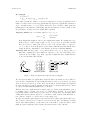
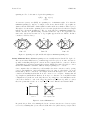
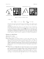
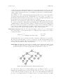
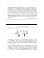
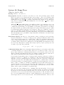
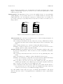
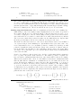
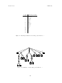
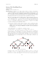
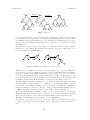
The last summation is probably the most important one for data structures. For example,
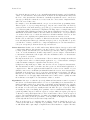
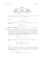
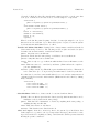
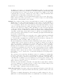
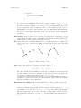
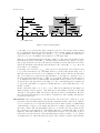
suppose you want to know how many nodes are in a complete 3-ary tree of height h. (We have
not given a formal definition of tree’s yet, but consider the figure below.
The height of a tree is the maximum number of edges from the root to a leaf.) One way to
break this computation down is to look at the tree level by level. At the top level (level 0)
there is 1 node, at level 1 there are 3 nodes, at level 2, 9 nodes, and in general at level i there
3i nodes. To find the total number of nodes we sum over all levels, 0 through h. Plugging into
the above equation with h = n we have:
h
X
i=0
3i =
3h+1 − 1
∈ O(3h ).
2
5
Lecture Notes
CMSC 420
Figure 1: Complete 3-ary tree of height 2.
Conversely, if someone told you that he had a 3-ary tree with n nodes, you could determine
the height by inverting this. Since n = (3(h+1) − 1)/2 then we have
3(h+1) = (2n + 1)
implying that
h = (log3 (2n + 1)) − 1 ∈ O(log n).
Another important fact to keep in mind about summations is that they can be approximated
using integrals.
Z b
b
X
f (i) ≈
f (x)dx.
x=a
i=a
Given an obscure summation, it is often possible to find it in a book on integrals, and use the
formula to approximate the sum.
Recurrences: A second mathematical construct that arises when studying recursive programs (as
are many described in this class) is that of a recurrence. A recurrence is a mathematical
formula that is defined recursively. For example, let’s go back to our example of a 3-ary tree
of height h. There is another way to describe the number of nodes in a complete 3-ary tree.
If h = 0 then the tree consists of a single node. Otherwise that the tree consists of a root
node and 3 copies of a 3-ary tree of height h − 1. This suggests the following recurrence which
defines the number of nodes N (h) in a 3-ary tree of height h:
N (0)
=
1
N (h)
=
3N (h − 1) + 1
if h ≥ 1.
Although the definition appears circular, it is well grounded since we eventually reduce to
N (0).
N (1)
=
3N (0) + 1 = 3 · 1 + 1 = 4
N (2)
=
3N (1) + 1 = 3 · 4 + 1 = 13
N (3)
=
3N (2) + 1 = 3 · 13 + 1 = 40,
and so on.
There are two common methods for solving recurrences. One (which works well for simple
regular recurrences) is to repeatedly expand the recurrence definition, eventually reducing it
to a summation, and the other is to just guess an answer and use induction. Here is an example
of the former technique.
N (h)
= 3N (h − 1) + 1
= 3(3N (h − 2) + 1) + 1 = 9N (h − 2) + 3 + 1
6
Lecture Notes
CMSC 420
=
..
.
9(3N (h − 3) + 1) + 3 + 1 = 27N (h − 3) + 9 + 3 + 1
=
3k N (h − k) + (3k−1 + . . . + 9 + 3 + 1)
When does this all end? We know that N (0) = 1, so let’s set k = h implying that
N (h) = 3h N (0) + (3h−1 + . . . + 3 + 1) = 3h + 3h−1 + . . . + 3 + 1 =
h
X
3i .
i=0
This is the same thing we saw before, just derived in a different way.
Proofs by Induction: The last mathematical technique of importance is that of proofs by induction. Induction proofs are critical to all aspects of computer science and data structures, not
just efficiency proofs. In particular, virtually all correctness arguments are based on induction.
From courses on discrete mathematics you have probably learned about the standard approach
to induction. You have some theorem that you want to prove that is of the form, “For all
integers n ≥ 1, blah, blah, blah”, where the statement of the theorem involves n in some way.
The idea is to prove the theorem for some basis set of n-values (e.g. n = 1 in this case), and
then show that if the theorem holds when you plug in a specific value n − 1 into the theorem
then it holds when you plug in n itself. (You may be more familiar with going from n to n + 1
but obviously the two are equivalent.)
In data structures, and especially when dealing with trees, this type of induction is not particularly helpful. Instead a slight variant called strong induction seems to be more relevant.
The idea is to assume that if the theorem holds for all values of n that are strictly less than n
then it is true for n. As the semester goes on we will see examples of strong induction proofs.
Let’s go back to our previous example problem. Suppose we want to prove the following
theorem.
Theorem: Let T be a complete 3-ary tree with n ≥ 1 nodes. Let H(n) denote the height of
this tree. Then
H(n) = (log3 (2n + 1)) − 1.
Basis Case: (Take the smallest legal value of n, n = 1 in this case.) A tree with a single node
has height 0, so H(1) = 0. Plugging n = 1 into the formula gives (log3 (2 · 1 + 1)) − 1
which is equal to (log3 3) − 1 or 0, as desired.
Induction Step: We want to prove the theorem for the specific value n > 1. Note that we
cannot apply standard induction here, because there is no complete 3-ary tree with 2
nodes in it (the next larger one has 4 nodes).
We will assume the induction hypothesis, that for all smaller n0 , 1 ≤ n0 < n, H(n0 ) is
given by the formula above. (This is sometimes called strong induction, and it is good to
learn since most induction proofs in data structures work this way.)
Let’s consider a complete 3-ary tree with n > 1 nodes. Since n > 1, it must consist of
a root node plus 3 identical subtrees, each being a complete 3-ary tree of n0 < n nodes.
How many nodes are in these subtrees? Since they are identical, if we exclude the root
node, each subtree has one third of the remaining number nodes, so n0 = (n − 1)/3. Since
n0 < n we can apply the induction hypothesis. This tells us that
H(n0 )
=
(log3 (2n0 + 1)) − 1 = (log3 (2(n − 1)/3 + 1)) − 1
7
Lecture Notes
CMSC 420
=
(log3 (2(n − 1) + 3)/3) − 1 = (log3 (2n + 1)/3) − 1
=
log3 (2n + 1) − log3 3 − 1 = log3 (2n + 1) − 2.
Note that the height of the entire tree is one more than the heights of the subtrees so
H(n) = H(n0 ) + 1. Thus we have:
H(n) = log3 (2n + 1) − 2 + 1 = log3 (2n + 1) − 1,
as desired.
This may seem like an awfully long-winded way of proving such a simple fact. But induction
is a very powerful technique for proving many more complex facts that arise in data structure
analyses.
You need to be careful when attempting proofs by induction that involve O(n) notation. Here
is an example of a common error.
False! Theorem: For n ≥ 1, let T (n) be given by the following summation
T (n) =
n
X
i,
i=0
then T (n) ∈ O(n). (We know from the formula for the linear series above that T (n) =
n(n + 1)/2 ∈ O(n2 ). So this must be false. Can you spot the error in the following
“proof”?)
Basis Case: For n = 1 we have T (1) = 1, and 1 is O(1).
Induction Step: We want to prove the theorem for the specific value n > 1. Suppose that
for any n0 < n, T (n0 ) ∈ O(n0 ). Now, for the case n, we have (by definition)
!
n
n−1
X
X
i =
i + n = T (n − 1) + n.
T (n) =
i=0
i=0
Now, since n−1 < n, we can apply the induction hypothesis, giving T (n−1) ∈ O(n−1).
Plugging this back in we have
T (n) ∈ O(n − 1) + n.
But (n − 1) + n ≤ 2n − 1 ∈ O(n), so we have T (n) ∈ O(n).
What is the error? Recall asymptotic notation applies to arbitrarily large n (for n in the limit).
However induction proofs by their very nature only apply to specific values of n. The proper
way to prove this by induction would be to come up with a concrete expression, which does
not involve O-notation. For example, try to prove that for all n ≥ 1, T (n) ≤ 50n. If you
attempt to prove this by induction (try it!) you will see that it fails.
Lecture 3: A Quick Introduction to Java
(Tuesday, Feb 6, 2001)
Read: Chapt 1 of Weiss (from 1.4 to the end).
Disclaimer: I am still learning Java, and there is a lot that I do not know. If you spot any errors
in this lecture, please bring them to my attention.
8
Lecture Notes
CMSC 420
Overview: This lecture will present a very quick description of the Java language (at least the
portions that will be needed for the class projects. The Java programming language has a
number of nice features, which make it an excellent programming language for implementing
data structures. Based on my rather limited experience with Java, I find it to be somewhat
cleaner and easier than C++ for data structure implementation (because of its cleaner support
for strings, exceptions and threads, its automatic memory management, and its more integrated
view of classes). Nonetheless, there are instances where C++ would be better choice than Java
for implementation (because of its template capability, its better control over memory layout
and memory management).
Java API: The Java language is very small and simple compared to C++. However, it comes with
a very large and constantly growing library of utility classes. Fortunately, you only need to
know about the parts of this library that you need, and the documentation is all online. The
libraries are grouped into packages, which altogether are called the “Java 2 Platform API”
(application programming interface). Some examples of these packages include
java.lang: Contains things like strings, that are essentially built in to the language.
java.io: Contains support for input and output, and
java.util: Contains some handy data structures such as lists and hash tables.
Simple Types: The basic elements of Java and C++ are quite similar. Both languages use the
same basic lexical structure and have the same methods for writing comments. Java supports
the following simple types, from which more complex types can be constructed.
Integer types: These include byte (8-bit), short (16-bit), int (32-bit), and long (64-bit).
All are signed integers.
Floating point types: These include float (32-bit) and double (64-bit).
Characters: The char type is a 16-bit unicode character (unlike C++ where it behaves
essentially like a byte.)
Booleans: The boolean type is the analogue to C++’s bool, either true or false.
Variables, Literals, and Casting: Variable declarations, literals (constants) and casting work
much like they do in C++.
int i = 10 * 4;
byte j = (byte) i;
long l = i;
float pi1 = 3.14f;
double pi2 = 3.141593653;
char c = ’a’;
boolean b = (i < pi1);
//
//
//
//
integer assignment
example of a cast
cast not needed when "widening"
floating assignment
// character
// boolean
All the familiar arithmetic operators are just as they are in C++.
Arrays: In C++ an array is just a pointer to its first element. There is no index range checking at
run time. In Java, arrays have definite lengths and run-time index checking is done. They are
indexed starting from 0 just as in C++. When an array is declared, no storage is allocated.
Instead, storage is allocated by using the new operator, as shown below.
int A[];
A = new int[4] = {12, 4, -6, 41};
char B[][] = new char[3][8];
B[0][3] = ’c’;
// A is an array, initially null
// this allocates and defines array
// B is a 2-dim, 3 x 8 array of char
9
Lecture Notes
CMSC 420
In Java you do not need to delete things created by new. It is up to the system to do garbage
collection to get rid of objects that you no longer refer to. In Java a 2-dimension array is
actually an array of arrays.
String Object: In C++ a string is implemented as an array of characters, terminated by a null
character. Java has much better integrated support for strings, in terms of a special String
object. For example, each string knows its length. Strings can be concatenated using the “+”
operator (which is the only operator overloading supported in Java).
String S = "abc";
String T = S + "def";
char c = T[3];
S = S + T;
int k = T.length();
//
//
//
//
//
S is the string "abc"
T is the string "abcdef"
c = ’d’
now S = "abcabcdef"
k = 6
Note that strings can be appended to by concatenation (as shown above with S). If you plan
on making many changes to a string variable, there is a type StringBuffer which provides a
more efficient method for “growable” strings.
Java supports automatic casting of simple types into strings, which comes in handy for doing
output. For example,
int cost = 25;
String Q = "The value is " + cost + " dollars";
Would set Q to “The value is 25 dollars”. If you define your own object, you can define a method
toString(), which produces a String representation for your object. Then any attempt to
cast your object to a string will invoke your method.
There are a number of other string functions that are supported. One thing to watch out for is
string comparison. The standard == operator will not do what you might expect. The reason
is that a String object (like all objects in Java) behaves much like a pointer or reference does in
C++. Comparisons using == test whether the pointers are the same, not whether the contents
are the same. The equals() or compareTo() methods to test the string contents.
Flow Control: All the standard flow-control statements, if-then-else, for, while, switch,
continue, etc., are the same as in C++.
Standard I/O: Input and output from the standard input/output streams are not quite as simple
in Java as in C++. Output is done by the print() and println() methods, each of which
prints a string to the standard output. The latter prints an end-of-line character. In Java
there are no global variables or functions. Everything is referenced as a member of some
object. These functions exist as part of the System.out object. Here is an example of its
usage.
int age = 12;
System.out.println("He is " + age + " years old");
Input in Java is much messier. Since our time is limited, we’ll refer you to our textbook (by
Weiss) for an example of how to use the java.io.BufferedReader, java.io.InputStreamReader, StringTokenizer to input lines and read them into numeric, string, and character
variables.
10
Lecture Notes
CMSC 420
Classes and Objects: Virtually everything in Java is organized around the notion of hierarchy of
objects and classes. As in C++ an object is an entity which stores data and provides methods
for accessing and modifying the data. An object is an instance of a class, which defines the
specifics of the object. As in C++ a class consists of instance variables and methods. Although
classes are superficially similar to classes in C++, there are some important differences in how
they operate.
File Structure: Java differs from C++ in that there is a definite relationship between files
and classes. Normally each Java class resides within its own file, whose name is derived from the name of the class. For example, a class Student would be stored in file
Student.java. Unlike C++, in which class declarations are stored in different files (.h
and .cc), in Java everything is stored in the same file and all definitions are made within
the class.
Packages: Another difference with C++ is the notion of packages. A package is a collection
of related classes (e.g. the various classes that make up one data structure). The classes
that make up a package are stored in a common directory (with the same name as the
package). In C++ you access predefined objects using an #include command to load the
definitions. In Java this is done by importing the desired package. For example, if you
wanted to use the Stack data structure in the java.util library, you would load this
using the following.
import java.util.Stack;
The Dot (.) Operator: Class members are accessed as in C++ using the dot operator.
However in Java, objects all behave as if they were pointers (or perhaps more accurately
as references that are allowed to be null).
class Person {
String name;
int
age;
public Person() {...}
}
Person p;
p = new Person();
Person q = p;
p = null;
// constructor (details omitted)
//
//
//
//
p
p
q
q
has the value null
points to a new object
and p now point to the same object
still points to the object
Note that unlike C++ the declaration “Person p” did not allocate an object as it would
in C++. It creates a null pointer to a Person. Objects are only created using the “new”
operator. Also, unlike C++ the statement “q = p” does not copy the contents of p,
but instead merely assigns the pointer q to point to the same object as p. Note that
the pointer and reference operators of C++ (“*”, “&”, “->”) do not exist in Java (since
everything is a pointer).
While were at it, also note that there is no semicolon (;) at the end of the class definition.
This is one small difference between Java and C++.
Inheritance and Subclasses: As with C++, Java supports class inheritance (but only single
not multiple inheritance). A class which is derived from another class is said to be a child
or subclass, and it is said to extend the original parent class, or superclass.
class Person { ... }
class Student extends Person { ... }
The Student class inherits the structure of the Person class and can add new instance
variables and new methods. If it redefines a method, then this new method overrides the
11
Lecture Notes
CMSC 420
old method. Methods behave like virtual member functions in C++, in the sense that
each object “remembers” how it was created, even if it assigned to a superclass.
class Person {
public void print() { System.out.println("Person"); }
}
class Student extends Person {
public void print() { System.out.println("Student"); }
}
Person P = new Person();
Student S = new Student();
Person Q = S;
Q.print();
What does the last line print? It prints “Student”, because Q is assigned to an object
that was created as a Student object. This called dynamic dispatch, because the system
decides at run time which function is to be called.
Variable and Method Modifiers: Getting back to classes, instance variables and methods
behave much as they do in C++. The following variable modifiers and method modifiers
determine various characteristics of variables and methods.
public: Any class can access this item.
protected: Methods in the same package or subclasses can access this item.
private: Only this class can access this item.
static: There is only one copy of this item, which is shared between all instances of the
class.
final: This item cannot be overridden by subclasses. (This is allows the compiler to
perform optimizations.)
abstract: (Only for methods.) This is like a pure virtual method in C++. This method
is not defined here (no code is provided), but rather must be defined by a subclass.
Note that Java does not have const variables like C++, nor does it have enumerations. A
constant is defined as a static final variable. (Enumerations can be faked by defining
many constants.)
class Person {
static final int TALL
= 0;
static final int MEDIUM = 1;
static final int SHORT = 2;
...
}
Class Modifiers: Unlike C++, classes can also be associated with modifiers.
(Default:) If no modifier is given then the class is friendly, which means that it can be
instantiated only by classes in the same package.
public: This class can be instantiated or extended by anything in the same package or
anything that imports this class.
final: This class can have no subclasses.
abstract: This class has some abstract methods.
“this” and “super”: As in C++, this is a pointer to the current object. In addition, Java
defines super to be a pointer to the object’s superclass. The super pointer is nice because
it provides a method for explicitly accessing overridden methods in the parent’s class and
invoking the parent’s constructor.
12
Lecture Notes
CMSC 420
class Person {
int age;
public Person(int a) { age = a; }
}
class Student extends Person {
String major;
public Student(int a, String m) {
super(a);
major = m;
}
}
// Person constructor
// Student constructor
// construct Person
(By the way, this is a dangerous way to initialize a String object, since recall that assignment does not copy contents, it just copies the pointer.)
Functions, Parameters, and Wrappers: Unlike C++ all functions must be part of some class.
For example, the main procedure must itself be declared as part of some class, as a public,
static, void method. The command line arguments are passed in as an array of strings. Since
arrays can determine their own length from the length() method, there is no need to indicate
the number of arguments. For example, here is what a typical Hello-World program would
look like. This is stored in a file HelloWorld.java
class HelloWorld {
public static void main(String args[]) {
System.out.println("Hello World");
System.out.println("The number of arguments is " + args.length());
}
}
In Java simple types are passed by value and objects are passed by reference. Thus, modifying
an object which has been passed in through a parameter of the function has the effect of
modifying the original object in the calling routine.
What if you want to pass an integer to a function and have its value modified. Java provides
a simple trick to do this. You simply wrap the integer with a class, and now it is passed
by reference. Java efines wrapper classes Integer (for int), Long, Character (for char),
Boolean, etc.
Generic Data Structures without Templates: Java does not have many of the things that
C++ has, templates for example. So, how do you define a generic data structure (e.g. a
Stack) that can contain objects of various types (int, float, Person, etc.)? In Java every class
automatically extends a most generic class called Object. We set up our generic stack to hold
objects of type Object. Since this is a superclass of all classes, we can store any objects from
any class in our stack. Of course, to keep our sanity, we should store object of only one type
in any given stack. (Since it will be very difficulty to figure out what comes out whenever we
pop something off the stack.)
Consider the ArrayVector class defined below. Suppose we want to store integers in this
vector. An int is not an object, but we can use the wrapper class Integer to convert an
integer into an object.
ArrayVector A = new ArrayVector();
A.insertAtRank(0, Integer(999));
A.insertAtRank(1, Integer(888));
Integer x = (Integer) A.elemAtRank(0);
13
// insert 999 at position 0
// insert 888 at position 1
// accesses 999
Lecture Notes
CMSC 420
Note that the ArrayVector contains Objects. Thus, when we access something from the data
structure, we need to cast it back to the appropriate type.
// This is an example of a simple Java class, which implements a vector
// object using an array implementation. This would be stored in a file
// named "ArrayVector.java".
public class ArrayVector {
private Object[] a;
private int capacity = 16;
private int size = 0;
// Array storing the elements of the vector
// Length of array a
// Number of elements stored in the vector
// Constructor
public ArrayVector() { a = new Object[capacity]; }
// Accessor methods
public Object elemAtRank(int r) { return a[r]; }
public int size() { return size; }
public boolean isEmpty() { return size() == 0; }
// Modifier methods
public Object replaceAtRank(int r, Object e) {
Object temp = a[r];
a[r] = e;
return temp;
}
public Object removeAtRank(int r) {
Object temp = a[r];
for (int i=r; i < size-1; i++)
a[i] = a[i+1];
size--;
return temp;
}
// Shift elements down
public void insertAtRank(int r, Object e) {
if (size == capacity) {
// An overflow
capacity *= 2;
Object[] b = new Object[capacity];
for (int i=0; i < size; i++)
b[i] = a[i];
a = b;
}
for (int i=size-1; i>=r; i--)
// Shift elements up
a[i+1] = a[i];
a[r] = e;
size++;
}
}
Lecture 4: Basic Data Structures
(Thursday, Feb 8, 2001)
14
Lecture Notes
CMSC 420
Read: Chapt. 3 in Weiss.
Basic Data Structures: Before we go into our coverage of complex data structures, it is good to
remember that in many applications, simple data structures are sufficient. This is true, for
example, if the number of data objects is small enough that efficiency is not so much an issue,
and hence a complex data structure is not called for. In many instances where you need a
data structure for the purposes of prototyping an application, these simple data structures are
quick and easy to implement.
Abstract Data Types: An important element to good data structure design is to distinguish
between the functional definition of a data structure and its implementation. By an abstract
data structure (ADT) we mean a set of objects and a set of operations defined on these objects.
For example, a stack ADT is a structure which supports operations such as push and pop (whose
definition you are no doubt familiar with). A stack may be implemented in a number of ways,
for example using an array or using a linked list. An important aspect of object oriented
languages like C++ and Java is the capability to present the user of a data structure with an
abstract definition of its function without revealing the methods with which it operates. To
a large extent, this course will be concerned with the various options for implementing simple
abstract data types and the tradeoffs between these options.
Linear Lists: A linear list or simply list is perhaps the most basic abstract data types. A list is
simply an ordered sequence of elements ha1 , a2 , . . . , an i. We will not specify the actual type of
these elements here, since it is not relevant to our presentation. (In C++ this might be done
through the use of templates. In Java this can be handled by defining the elements to be of
type Object. Since the Object class is a superclass of all other classes, we can store any class
type in our list.)
The size or length of such a list is n. There is no agreed upon specification of the list ADT,
but typical operations include:
get(i): Returns element ai .
set(i,x): Sets the ith element to x.
length(): Returns the length of the list.
insert(i,x): Insert element x just prior to element ai (causing the index of all subsequent
items to be increased by one).
delete(i): Delete the ith element (causing the indices of all subsequent elements to be decreased by 1).
I am sure that you can imagine many other useful operations, for example search the list for
an item, split or concatenate lists, return a sublist, make the list empty. There are often a
number of programming language related operations, such as returning an iterator object for
the list. Lists of various types are among the most primitive abstract data types, and because
these are taught in virtually all basic programming classes we will not cover them in detail
here.
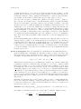
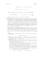
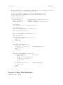
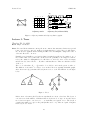
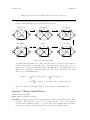
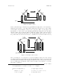
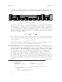
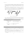
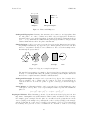
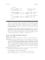
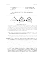
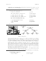
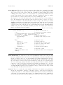
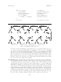
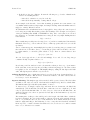
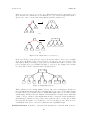
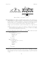
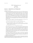
There are a number of possible implementations of lists. The most basic question is whether
to use sequential allocation (meaning storing the elements sequentially in an array) or linked
allocation (meaning storing the elements in a linked list. With linked allocation there are
many other options to be considered. Is the list singly linked, doubly linked, circularly linked?
Another question is whether we have an internal list, in which the nodes that constitute the
linked list contain the actual data items ai , or we have an external list, in which each linked
list item contains a pointer to the associated data item.
15
Lecture Notes
CMSC 420
a1
a2
a3
a4
head
a1
a2
a3
a4
head
a1
Sequential
allocation
Internal linked list
a2
a3
a4
External linked list
Figure 2: Common types of list allocation.
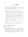
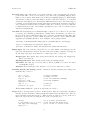
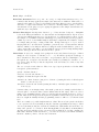
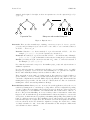
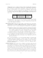
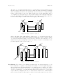
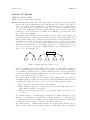
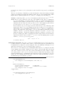
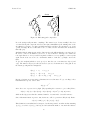
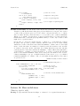
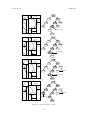
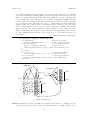
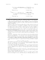
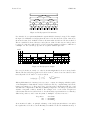
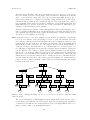
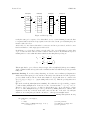
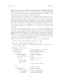
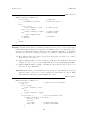
Multilists and Sparse Matrices: Although lists are very basic structures, they can be combined
in various nontrivial ways. One such example is the notion of a multilist, which can be thought
of as two sets of linked lists that are interleaved with each other. One application of multilists
is in representing sparse matrices. Suppose that you want to represent a very large m × n
matrix. Such a matrix can store O(mn) entries. But in many applications the number of
nonzero entries is much smaller, say on the order of O(m+n). (For example, if n = m = 10, 000
this might means that only around 0.01% of the entries are being used.) A common approach
for representing such a sparse matrix is by creating m linked lists, one for each row and n
linked lists, one for each column. Each linked list stores the nonzero entries of the matrix.
Each entry contains the row and column indices [i][j] as well as the value stored in this entry.
Columns
Matrix contents
0
85 0 67
15
0
0
99
0
22 39
0
0
1
Rows
0
1
2
0 1 85
0 3 67
1 0 15
1 3 99
2 1 22
2
3
2 2 39
Figure 3: Sparse matrix representation using multilists.
Stacks, Queues, and Deques: There are two very special types of lists: stacks and queues and
their generalization, called the deque.
Stack: Supports insertions (called pushes) and deletions (pops) from only one end (called
the top). Stacks are used often in processing tree-structured objects, in compilers (in
processing nested structures), and is used in systems to implement recursion.
Queue: Supports insertions (called enqueues) at one end (called the tail or rear) and deletions
(called dequeues) from the other end (called the head or front). Queues are used in
operating systems and networking to store a list of items that are waiting for some
resource.
Deque: This is a play on words. It is written like “d-e-que” for a “double-ended queue”, but
it is pronounced like deck, because it behaves like a deck of cards, where you can deal
off the top or the bottom. A deque supports insertions and deletions from either end.
Clearly, given a deque, you immediately have an implementation of a stack or queue by
simple inheritance.
16
Lecture Notes
CMSC 420
Both stacks and queues can be implemented efficiently as arrays or as linked lists. There are a
number of interesting issues involving these data structures. However, since you have probably
seen these already, we will skip the details here.
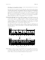
Graphs: Intuitively, a graph is a collection of vertices or nodes, connected by a collection of edges.
Graphs are extremely important because they are a very flexible mathematical model for many
application problems. Basically, any time you have a set of objects, and there is some “connection” or “relationship” or “interaction” between pairs of objects, a graph is a good way
to model this. Examples of graphs in application include communication and transportation
networks, VLSI and other sorts of logic circuits, surface meshes used for shape description in
computer-aided design and geographic information systems, precedence constraints in scheduling systems. The list of application is almost too long to even consider enumerating it.
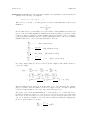
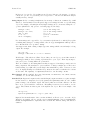
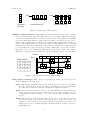
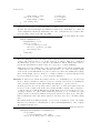
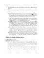
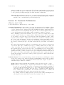
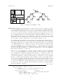
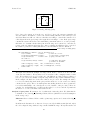
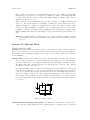
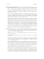
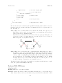
Definition: A directed graph (or digraph) G = (V, E) consists of a finite set V , called the
vertices or nodes, and E, a set of ordered pairs, called the edges of G. (Another way of
saying this is that E is a binary relation on V .)
Observe that self-loops are allowed by this definition. Some definitions of graphs disallow this.
Multiple edges are not permitted (although the edges (v, w) and (w, v) are distinct).
1
4
1
3
2
3
2
4
Digraph
Graph
Figure 4: Digraph and graph example.
Definition: An undirected graph (or graph) G = (V, E) consists of a finite set V of vertices,
and a set E of unordered pairs of distinct vertices, called the edges. (Note that self-loops
are not allowed).
Note that directed graphs and undirected graphs are different (but similar) objects mathematically. We say that vertex v is adjacent to vertex u if there is an edge (u, v). In a directed
graph, given the edge e = (u, v), we say that u is the origin of e and v is the destination of e.
In undirected graphs u and v are the endpoints of the edge. The edge e is incident (meaning
that it touches) both u and v.
In a digraph, the number of edges coming out of a vertex is called the out-degree of that vertex,
and the number of edges coming in is called the in-degree. In an undirected graph we just talk
about the degree of a vertex as the number of incident edges. By the degree of a graph, we
usually mean the maximum degree of its vertices.
When discussing the size of a graph, we typically consider both the number of vertices and
the number of edges. The number of vertices is typically written as n or V , and the number
of edges is written as m or E. Here are some basic combinatorial facts about graphs and
digraphs. We will leave the proofs to you. Given a graph with V vertices and E edges then:
In a graph:
• 0 ≤ E ≤ n2 = n(n − 1)/2 ∈ O(n2 ).
P
•
v∈V deg(v) = 2E.
17
Lecture Notes
CMSC 420
In a digraph:
• 0 ≤ E ≤ n2 .
P
P
•
v∈V in-deg(v) =
v∈V out-deg(v) = E.
Notice that generally the number of edges in a graph may be as large as quadratic in the
number of vertices. However, the large graphs that arise in practice typically have much fewer
edges. A graph is said to be sparse if E ∈ O(V ), and dense, otherwise. When giving the
running times of algorithms, we will usually express it as a function of both V and E, so that
the performance on sparse and dense graphs will be apparent.
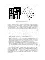
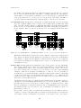
Adjacency Matrix: An n × n matrix defined for 1 ≤ v, w ≤ n.
1
if (v, w) ∈ E
A[v, w] =
0
otherwise.
If the digraph has weights we can store the weights in the matrix. For example if (v, w) ∈
E then A[v, w] = W (v, w) (the weight on edge (v, w)). If (v, w) ∈
/ E then generally
W (v, w) need not be defined, but often we set it to some “special” value, e.g. A(v, w) =
−1, or ∞. (By ∞ we mean (in practice) some number which is larger than any allowable
weight. In practice, this might be some machine dependent constant like MAXINT.)
Adjacency List: An array Adj[1 . . . n] of pointers where for 1 ≤ v ≤ n, Adj[v] points to a
linked list containing the vertices which are adjacent to v (i.e. the vertices that can be
reached from v by a single edge). If the edges have weights then these weights may also
be stored in the linked list elements.
1
2
Adj
1
1
1
2
1
3
1
1
1
2
0
0
1
2
3
3
0
1
0
3
2
2
3
3
Adjacency matrix
Adjacency list
Figure 5: Adjacency matrix and adjacency list for digraphs.
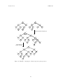
We can represent undirected graphs using exactly the same representation, but we will store
each edge twice. In particular, we representing the undirected edge {v, w} by the two oppositely
directed edges (v, w) and (w, v). Notice that even though we represent undirected graphs in
the same way that we represent digraphs, it is important to remember that these two classes
of objects are mathematically distinct from one another.
This can cause some complications. For example, suppose you write an algorithm that operates
by marking edges of a graph. You need to be careful when you mark edge (v, w) in the
representation that you also mark (w, v), since they are both the same edge in reality. When
dealing with adjacency lists, it may not be convenient to walk down the entire linked list, so
it is common to include cross links between corresponding edges.
An adjacency matrix requires O(V 2 ) storage and an adjacency list requires O(V + E) storage.
The V arises because there is one entry for each vertex in Adj . Since each list has out-deg(v)
entries, when this is summed over all vertices, the total number of adjacency list records is
O(E). For sparse graphs the adjacency list representation is more space efficient.
18
Lecture Notes
CMSC 420
Adj
1
4
2
3
1
1
0
2
1
3
1
4
1
2
1
0
1
0
3
1
1
0
1
4
1
0
1
0
Adjacency matrix
1
2
3
2
1
3
3
1
2
4
1
4
4
3
Adjacency list (with crosslinks)
Figure 6: Adjacency matrix and adjacency list for graphs.
Lecture 5: Trees
(Tuesday, Feb 13, 2001)
Read: Chapt. 4 in Weiss.
Trees: Trees and their variants are among the most common data structures. In its most general
form, a free tree is a connected, undirected graph that has no cycles. Since we will want to
use our trees for applications in searching, it will be more meaningful to assign some sense of
order and direction to our trees.
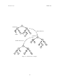
Formally a tree (actually a rooted tree) is defined recursively as follows. It consists of one or
more items called nodes. (Our textbook allows for the possibility of an empty tree with no
nodes.) It consists of a distinguished node called the root, and a set of zero or more nonempty
subsets of nodes, denoted T1 , T2 , . . . , Tk , where each is itself a tree. These are called the subtrees
of the root.
The root of each subtree T1 , . . . , Tk is said to be a child of r, and r is the parent of each root.
The children of r are said to be siblings of one another. Trees are typically drawn like graphs,
where there is an edge (sometimes directed) from a node to each of its children. See the figure
below.
A
r
B
T1
T2
. . .
Tk
C
F
E
H
D
G
I
Figure 7: Trees.
If there is an order among the Ti ’s, then we say that the tree is an ordered tree. The degree of
a node in a tree is the number of children it has. A leaf is a node of degree 0. A path between
two nodes is a sequence of nodes u1 , u2 , . . . , uk such that ui is a parent of ui+1 . The length of
a path is the number of edges on the path (in this case k − 1). There is a path of length 0
from every node to itself.
19
Lecture Notes
CMSC 420
The depth of a node in the tree is the length of the unique path from the root to that node.
The root is at depth 0. The height of a node is the length of the longest path from the node
to a leaf. Thus all leaves are at height 0. If there is a path from u to v we say that v is a
descendants of u. We say it is a proper descendent if u 6= v. Similarly, u is an ancestor of v.
Implementation of Trees: One difficulty with representing general trees is that since there is no
bound on the number of children a node can have, there is no obvious bound on the size of a
given node (assuming each node must store pointers to all its children). The more common
representation of general trees is to store two pointers with each node: the firstChild and
the nextSibling. The figure below illustrates how the above tree would be represented using
this technique.
root
nextSibling
data
firstChild
A
B
E
C
F
G
H
I
D
Figure 8: A binary representation of general trees.
Trees arise in many applications in which hierarchies exist. Examples include the Unix file
system, corporate managerial structures, and anything that can be described in “outline form”
(like the chapters, sections, and subsections of a user’s manual). One special case of trees will
be very important for our purposes, and that is the notion of a binary tree.
Binary Trees: Our text defines a binary tree as a tree in which each node has no more than two
children. However, this definition is subtly flawed. A binary tree is defined recursively as
follows. A binary tree can be empty. Otherwise, a binary tree consists of a root node and two
disjoint binary trees, called the left and right subtrees. The difference in the two definitions
is important. There is a distinction between a tree with a single left child, and one with a
single right child (whereas in our normal definition of tree we would not make any distinction
between the two).
The typical Java representation of a tree as a data structure is given below. The element field
contains the data for the node and is of some abstract type, which in Java might be Object.
(In C++ the element type could be specified using a template.) When we need to be concrete
we will often assume that element fields are just integers. The left field is a pointer to the
left child (or null if this tree is empty) and the right field is analogous for the right child.
class BinaryTreeNode {
Object
element;
BinaryTreeNode left;
BinaryTreeNode right;
...
}
// data item
// left child
// right child
Binary trees come up in many applications. One that we will see a lot of this semester
is for representing ordered sets of objects, a binary search tree. Another one that is used
often in compiler design is expression trees which are used as an intermediate representation
for expressions when a compiler is parsing a statement of some programming language. For
20
Lecture Notes
CMSC 420
example, in the figure below right, we show an expression tree for the expression ((a + b) ∗
c)/(d − e)).
/
B
−
*
+
a
c
d
B
C
A
e
D
C
A
D
b
Expression Tree
Binary tree and extended binary tree
Figure 9: Expression tree.
Traversals: There are three natural ways of visiting or traversing every node of a tree, preorder,
postorder, and (for binary trees) inorder. Let T be a tree whose root is r and whose subtrees
are T1 , T2 , . . . , Tm for m ≥ 0.
Preorder: Visit the root r, then recursively do a preorder traversal of T1 , T2 , . . . , Tk . For
example: h/, ∗, +, a, b, c, −, d, ei for the expression tree shown above.
Postorder: Recursively do a postorder traversal of T1 , T2 , . . . , Tk and then visit r. Example:
ha, b, +, c, ∗, d, e, −, /i. (Note that this is not the same as reversing the preorder traversal.)
Inorder: (for binary trees) Do an inorder traversal of TL , visit r, do an inorder traversal of
TR . Example: ha, +, b, ∗, c, /, d, −, ei.
Note that theses traversal correspond to the familiar prefix, postfix, and infix notations for
arithmetic expressions.
Preorder arises in game-tree applications in AI, where one is searching a tree of possible
strategies by depth-first search. Postorder arises naturally in code generation in compilers.
Inorder arises naturally in binary search trees which we will see more of.
These traversals are most easily coded using recursion. If recursion is not desired (either for
greater efficiency or for fear of using excessive system stack space) it is possible to use your
own stack to implement the traversal. Either way the algorithm is quite efficient in that its
running time is proportional to the size of the tree. That is, if the tree has n nodes then the
running time of these traversal algorithms are all O(n).
Extended Binary Trees: Binary trees are often used in search applications, where the tree is
searched by starting at the root and then proceeding either to the left or right child, depending
on some condition. In some instances the search stops at a node in the tree. However, in some
cases it attempts to cross a null link to a nonexistent child. The search is said to “fall out” of
the tree. The problem with falling out of a tree is that you have no information of where this
happened, and often this knowledge is useful information. Given any binary tree, an extended
binary tree is one which is formed by replacing each missing child (a null pointer) with a special
leaf node, called an external node. The remaining nodes are called internal nodes. An example
is shown in the figure above right, where the external nodes are shown as squares and internal
nodes are shown as circles. Note that if the original tree is empty, the extended tree consists
of a single external node. Also observe that each internal node has exactly two children and
each external node has no children.
21
Lecture Notes
CMSC 420
Let n denote the number of internal nodes in an extended binary tree. Can we predict how
many external nodes there will be? It is a bit surprising but the answer is yes, and in fact
the number of extended nodes is n + 1. The proof is by induction. This sort of induction is
so common on binary trees, that it is worth going through this simple proof to see how such
proofs work in general.
Claim: An extended binary tree with n internal nodes has n + 1 external nodes.
Proof: By (strong) induction on the size of the tree. Let X(n) denote the number of external
nodes in a binary tree of n nodes. We want to show that for all n ≥ 0, X(n) = n + 1.
The basis case is for a binary tree with 0 nodes. In this case the extended tree consists
of a single external node, and hence X(0) = 1.
Now let us consider the case of n ≥ 1. By the induction hypothesis, for all 0 ≤ n0 < n, we
have X(n0 ) = n0 + 1. We want to show that it is true for n. Since n ≥ 1 the tree contains
a root node. Among the remaining n − 1 nodes, some number k are in the left subtree,
and the other (n − 1) − k are in the right subtree. Note that k and (n − 1) − k are both
less than n and so we may apply the induction hypothesis. Thus, there are X(k) = k + 1
external nodes in the left subtree and X((n − 1) − k) = n − k external nodes in the right
subtree. Summing these we have
X(n) = X(k) + X((n − 1) − k) = (k + 1) + (n − k) = n + 1,
which is what we wanted to show.
Remember this general proof structure. When asked to prove any theorem on binary trees by
induction, the same general structure applies.
Complete Binary Trees: We have discussed linked allocation strategies for general trees and
binary trees. Is it possible to allocate trees using sequential (that is, array) allocation? In
general it is not possible because of the somewhat unpredictable structure of trees. However,
there is a very important case where sequential allocation is possible.
Complete Binary Tree: is a binary tree in which every level of the tree is completely filled,
except possibly the bottom level, which is filled from left to right.
It is easy to verify that a complete binary tree of height h has between 2h and 2h+1 − 1 nodes,
implying that a tree with n nodes has height O(log n). (We leave these as exercises involving
geometric series.) An example is provided in the figure below.
The extreme regularity of complete binary trees allows them to be stored in arrays, so no
additional space is wasted on pointers. Consider an indexing of nodes of a complete tree from
1 to n in increasing level order (so that the root is numbered 1 and the last leaf is numbered
n). Observe that there is a simple mathematical relationship between the index of a node and
the indices of its children and parents.
In particular:
leftChild(i): if (2i ≤ n) then 2i, else null.
rightChild(i): if (2i + 1 ≤ n) then 2i + 1, else null.
parent(i): if (i ≥ 2) then bi/2c, else null.
Observe that the last leaf in the tree is at position n, so adding a new leaf simply means
inserting a value at position n + 1 in the list and updating n.
22
Lecture Notes
CMSC 420
A
B
C
D
H
E
I
F
J
G
n = 10
max=15
A B C D E F G H I J
0 1 2 3 4 5 6 7 8 9 10 11 12 13 14 15
Figure 10: A complete binary tree.
Threaded Binary Trees: Note that binary tree traversals are defined recursively. Therefore a
straightforward implementation would require extra space to store the stack for the recursion.
The stack will save the contents of all the ancestors of the current node, and hence the additional space required is proportional to the height of the tree. (Either you do it explicitly or
the system handles it for you.) When trees are balanced (meaning that a tree with n nodes has
O(log n) height) this is not a big issue, because log n is so smaller compared to n. However,
with arbitrary trees, the height of the tree can be as high as n − 1. Thus the required stack
space can be considerable.
This raises the question of whether there is some way to traverse a tree without using additional
storage. There are two tricks for doing this. The first one involves altering the links in the tree
as we do the traversal. When we descend from parent to child, we reverse the parent-child link
to point from parent to the grandparent. These reversed links provide a way to back up the
tree when the recursion bottoms out. On backing out of the tree, we “unreverse” the links,
thus restoring the original tree structure. We will leave the details as an exercise.
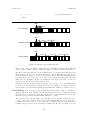
The second method involves a clever idea of using the space occupied for the null pointers
to store information to aid in the traversal. In particular, each left-child pointer that would
normally be null is set to the inorder predecessor of this node. Similarly each right-child pointer
that would normally be null is set to the inorder successor of this node. The resulting links
are called threads. This is illustrated in the figure below (where threads are shown as broken
curves).
Each such pointer needs to have a special “mark bit” to indicate whether it used as a parentchild link or as a thread. So the additional cost is only two bits per node. Now, suppose that
you are currently visiting a node u. How do we get to the inorder successor of u? If the right
child pointer is a thread, then we just follow it. Otherwise, we go the right child, and then
traverse left-child links until reaching the bottom of the tree (namely a threaded link).
BinaryTreeNode nextInOrder() {
BinaryTreeNode q = right;
if (rightIsThread) return q;
while (!q.leftIsThread) {
q = q.left;
}
return q;
}
//
//
//
//
//
//
23
inorder successor of "this"
go to right child
if thread, then done
else q is right child
go to left child
...until hitting thread
Lecture Notes
CMSC 420
D
D
B
A
B
I
C
F
E
A
J
I
C
F
E
G
J
G
H
H
Binary tree with threads
Binary tree
Figure 11: A Threaded Tree.
For example, in the figure below, suppose that we start with node A in each case. In the left
case, we immediately hit a thread, and return B as the result. In the right case, the right
pointer is not a thread, so we follow it to B, and then follow left links to C and D. But D’s left
child pointer is a thread, so we return D as the final successor. Note that the entire process
starts at the first node in an inorder traversal, that is, the leftmost node in the tree.
B
this A
B
C
this A
D
Figure 12: Inorder successor in a threaded tree.
Lecture 6: Minimum Spanning Trees and Prim’s Algorithm
(Thursday, Feb 15, 2001)
Read: Section 9.5 in Weiss.
Minimum Spanning Trees: A common problem in communications networks and circuit design
is that of connecting together a set of nodes (communication sites or circuit components) by a
network of minimal total length (where length is the sum of the lengths of connecting wires).
We assume that the network is undirected. To minimize the length of the connecting network,
it never pays to have any cycles (since we could break any cycle without destroying connectivity
and decrease the total length). Since the resulting connection graph is connected, undirected,
and acyclic, it is a free tree.
The computational problem is called the minimum spanning tree problem (MST for short).
More formally, given a connected, undirected graph G = (V, E), a spanning tree is an acyclic
subset of edges T ⊆ E that connects all the vertices together. Assuming that each edge (u, v)
of G has a numeric weight or cost, w(u, v), (may be zero or negative) we define the cost of a
24
Lecture Notes
CMSC 420
spanning tree T to be the sum of edges in the spanning tree
X
w(u, v).
w(T ) =
(u,v)∈T
A minimum spanning tree (MST) is a spanning tree of minimum weight. Note that the
minimum spanning tree may not be unique, but it is true that if all the edge weights are
distinct, then the MST will be distinct (this is a rather subtle fact, which we will not prove).
The figure below shows three spanning trees for the same graph, where the shaded rectangles
indicate the edges in the spanning tree. The one on the left is not a minimum spanning tree,
and the other two are. (An interesting observation is that not only do the edges sum to the
same value, but in fact the same set of edge weights appear in the two MST’s. Is this a
coincidence? We’ll see later.)
4
10
b
8
a
9
8
4
6
7
d
2
c
e
g
5
9
f
a
2
8
9
8
1
Cost = 33
10
b
d
4
6
7
2
c
e
g
5
9
f
2
1
Cost = 22
10
b
8
a
9
8
d
2
c
e
6
7
g
5
9
f
2
1
Cost = 22
Figure 13: Spanning trees (the middle and right are minimum spanning trees.
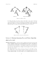
Steiner Minimum Trees: Minimum spanning trees are actually mentioned in the U.S. legal code.
The reason is that AT&T was a government supported monopoly at one time, and was responsible for handling all telephone connections. If a company wanted to connect a collection
of installations by an private internal phone system, AT&T was required (by law) to connect
them in the minimum cost manner, which is clearly a spanning tree . . . or is it?
Some companies discovered that they could actually reduce their connection costs by opening
a new bogus installation. Such an installation served no purpose other than to act as an
intermediate point for connections. An example is shown in the figure below. On the left,
consider four installations that that lie at the corners of a 1 × 1 square. Assume that all
edge lengths are just Euclidean distances. It is easy to see that the cost of any MST for this
configuration is 3 (as shown on the left). However, if you introduce
a new installation at the
√
2.
It
is
now possible to connect
center, whose distance to each of the other
four
points
is
1/
√
√
these five points with a total cost of of 4/ 2 = 2 2 ≈ 2.83. This is better than the MST.
MST
SMT
Steiner point
1
Cost = 3
Cost = 2 sqrt(2) = 2.83
Figure 14: Steiner Minimum tree.
In general, the problem of determining the lowest cost interconnection tree between a given
set of nodes, assuming that you are allowed additional nodes (called Steiner points) is called
25
Lecture Notes
CMSC 420
the Steiner minimum tree (or SMT for short). An interesting fact is that although there is a
simple greedy algorithm for MST’s (as we will see below), the SMT problem is much harder,
and in fact is NP-hard. (By the way, the US Legal code is rather ambiguous on the point as
to whether the phone company was required to use MST’s or SMT’s in making connections.)
Generic approach: We will present a greedy algorithm (called Prim’s algorithm) for computing a
minimum spanning tree. A greedy algorithm is one that builds a solution by repeated selecting
the cheapest (or generally locally optimal choice) among all options at each stage. An important characteristic of greedy algorithms is that once they make a choice, they never “unmake”
this choice. Before presenting these algorithms, let us review some basic facts about free trees.
They are all quite easy to prove.
Lemma:
• A free tree with n vertices has exactly n − 1 edges.
• There exists a unique path between any two vertices of a free tree.
• Adding any edge to a free tree creates a unique cycle. Breaking any edge on this
cycle restores a free tree.
Let G = (V, E) be an undirected, connected graph whose edges have numeric edge weights
(which may be positive, negative or zero). The intuition behind Prim’s algorithms is simple,
we maintain a subtree A of the edges in the MST. Initially this set is empty, and we will add
edges one at a time, until A equals the MST. We say that a subset A ⊆ E is viable if A is a
subset of edges in some MST (recall that it is not unique). We say that an edge (u, v) ∈ E − A
is safe if A ∪ {(u, v)} is viable. In other words, the choice (u, v) is a safe choice to add so that
A can still be extended to form an MST. Note that if A is viable it cannot contain a cycle.
Prim’s algorithm operates by repeatedly adding a safe edge to the current spanning tree.
When is an edge safe? We consider the theoretical issues behind determining whether an edge
is safe or not. Let S be a subset of the vertices S ⊆ V . A cut (S, V − S) is just a partition
of the vertices into two disjoint subsets. An edge (u, v) crosses the cut if one endpoint is in S
and the other is in V − S. Given a subset of edges A, we say that a cut respects A if no edge
in A crosses the cut. It is not hard to see why respecting cuts are important to this problem.
If we have computed a partial MST, and we wish to know which edges can be added that do
not induce a cycle in the current MST, any edge that crosses a respecting cut is a possible
candidate.
An edge of E is a light edge crossing a cut, if among all edges crossing the cut, it has the
minimum weight (the light edge may not be unique if there are duplicate edge weights).
Intuition says that since all the edges that cross a respecting cut do not induce a cycle, then
the lightest edge crossing a cut is a natural choice. The main theorem which drives both
algorithms is the following. It essentially says that we can always augment A by adding the
minimum weight edge that crosses a cut which respects A. (It is stated in complete generality,
so that it can be applied to both algorithms.)
MST Lemma: Let G = (V, E) be a connected, undirected graph with real-valued weights on
the edges. Let A be a viable subset of E (i.e. a subset of some MST), let (S, V − S) be
any cut that respects A, and let (u, v) be a light edge crossing this cut. Then the edge
(u, v) is safe for A.
Proof: It will simplify the proof to assume that all the edge weights are distinct. Let T be
any MST for G. If T contains (u, v) then we are done. Suppose that no MST contains
(u, v). We will derive a contradiction.
26
Lecture Notes
CMSC 420
9
u
4
u
v
4
4
u
v
v
7
x
6
x
x
8
8
y
y
T + (u,v)
A
y
T’ = T − (x,y) + (u,v)
w(T’) = w(T) − 8 + 4
Figure 15: MST Lemma.
Add the edge (u, v) to T , thus creating a cycle. Since u and v are on opposite sides of
the cut, and since any cycle must cross the cut an even number of times, there must be
at least one other edge (x, y) in T that crosses the cut.
The edge (x, y) is not in A (because the cut respects A). By removing (x, y) we restore
a spanning tree, call it T 0 . We have
w(T 0 ) = w(T ) − w(x, y) + w(u, v).
Since (u, v) is lightest edge crossing the cut, we have w(u, v) < w(x, y). Thus w(T 0 ) <
w(T ). This contradicts the assumption that T was an MST.
Prim’s Algorithm: There are two well-known greedy algorithms for computing MST’s: Prim’s
algorithm and Kruskal’s algorithm. We will discuss Prim’s algorithm here. Prim’s algorithm
runs in O((V + E) log V ) time. Prim’s algorithm builds the tree up by adding leaves one at a
time to the current tree. We start with a root vertex r (it can be any vertex). At any time,
the subset of edges A forms a single tree. We look to add a single vertex as a leaf to the tree.
The process is illustrated in the following figure.
12
12
10
10
6
r
r
7
7
11
4
6
3
u
u
5
9
5
Figure 16: Prim’s Algorithm.
Observe that if we consider the set of vertices S currently part of the tree, and its complement
(V − S), we have a cut of the graph and the current set of tree edges A respects this cut.
Which edge should we add next? The MST Lemma from the previous lecture tells us that it
is safe to add the light edge. In the figure, this is the edge of weight 4 going to vertex u. Then
27
Lecture Notes
CMSC 420
u is added to the vertices of S, and the cut changes. Note that some edges that crossed the
cut before are no longer crossing it, and others that were not crossing the cut are.
It is easy to see, that the key questions in the efficient implementation of Prim’s algorithm is
how to update the cut efficiently, and how to determine the light edge quickly. To do this, we
will make use of a priority queue data structure. Recall that this is the data structure used
in HeapSort. This is a data structure that stores a set of items, where each item is associated
with a key value. The priority queue supports three operations.
ref = insert(u, key): Insert vertex u with the key value key in the priority queue. The
operation returns a pointer ref to allow future access to this item.
u = extractMin(): Extract the vertex with the minimum key value in Q.
decreaseKey(ref, newKey): Decrease the value of the entry with the given reference ref.
The new key value is newKey.
A priority queue can be implemented using the same heap data structure used in heapsort.
The above operations can be performed in O(log n) time, where n is the number of items in the
heap. Some care needs to be taken in how references are handled. The various heap operations
cause items in the heap to be moved around. But the references cannot be moved, because
they are our only way of accessing heap nodes from the outside. This can be done by having
the heap store pointers to the reference objects.
What do we store in the priority queue? At first you might think that we should store the
edges that cross the cut, since this is what we are removing with each step of the algorithm.
The problem is that when a vertex is moved from one side of the cut to the other, this results
in a complicated sequence of updates.
There is a much more elegant solution, and this is what makes Prim’s algorithm so nice. For
each vertex in u ∈ V − S (not part of the current spanning tree) we associate u with a key
value key[u], which is the weight of the lightest edge going from u to any vertex in S. We
also store in pred[u] the end vertex of this edge in S. If there is not edge from u to a vertex
in V − S, then we set its key value to +∞. We will also need to know which vertices are in S
and which are not. We do this by coloring the vertices in S black.
Here is Prim’s algorithm. The root vertex r can be any vertex in V .
Prim’s Algorithm
Prim(Graph G, Vertex r) {
for each (u in V) {
// initialization
key[u] = +infinity;
color[u] = white;
pred[u] = null;
}
key[r] = 0;
// start at root
Q = new PriQueue(V);
// put vertices in Q
while (Q.nonEmpty()) {
// until all vertices in MST
u = Q.extractMin();
// vertex with lightest edge
for each (v in Adj[u]) {
if ((color[v] == white) && (w(u,v) < key[v])) {
key[v] = w(u,v);
// new lighter edge out of v
Q.decreaseKey(v, key[v]);
pred[v] = u;
}
}
color[u] = black;
28
Lecture Notes
CMSC 420
}
[The pred pointers define the MST as an inverted tree rooted at r]
}
The following figure illustrates Prim’s algorithm. The arrows on edges indicate the predecessor
pointers, and the numeric label in each vertex is the key value.
4
8
Q: 4,8,?,?,?,?
10
4
?
6
8 7
9
5 ?
?
9
2
2
8
?
1
Q: <empty>
10
4
8
8
9
2
4
8
5
Q: 8,8,10,?,?
10
10
6
8 7
9
5 ?
8
9
2
2
8
?
1
Q: 2,5
10
2
4
6
7
9
4
5
8
2
8
1
5
9
2
4
8
Q: 1,2,10,?
10
10
6
8 7
9
5 ?
2
9
2
2
1
1
1
Q: 2,2,5
10
2
4
6
7
9
8
5
9
2
2
8
8
5
6
7
2
2
9
5
2
2
1
1
Figure 17: Prim’s Algorithm.
To analyze Prim’s algorithm, we account for the time spent on each vertex as it is extracted
from the priority queue. It takes O(log V ) to extract this vertex from the queue. For each
incident edge, we spend potentially O(log V ) time decreasing the key of the neighboring vertex.
Thus the time is O(log V + deg(u) log V ) time. The other steps of the update are constant
time. So the overall running time is
T (V, E)
=
X
(log V + deg(u) log V ) =
u∈V
=
log V
X
X
(1 + deg(u)) log V
u∈V
(1 + deg(u)) = (log V )(V + 2E) = Θ((V + E) log V ).
u∈V
Since G is connected, V is asymptotically no greater than E, so this is Θ(E log V ).
Lecture 7: Binary Search Trees
(Tuesday, Feb 20, 2001)
Read: Chapt 4 of Weiss, through 4.3.6.
Searching: Searching is among the most fundamental problems in data structure design. Traditionally, we assume that we are given a set of elements {E1 , E2 , . . . , En }, where each Ei is
associated with a distinct key value, xi over some totally ordered domain. Given an arbitrary
search key x, we wish to determine whether there is a element containing this key.
29
Lecture Notes
CMSC 420
Assuming that each object contains a key field is sometimes a bit awkward (since it may involve
accessing private data). A somewhat more attractive way to handle this in modern languages
like C++ and Java is to assume that the element E has a comparison method defined for it.
(In Java we would say that the object is a subclass of type Comparable.) This means that
the class provides a method int compareTo(), whose argument is of the same type as this
class. Since we are not constrained to using one programming language, we will allow ourselves
to overload the comparison operators (which Java does not permit) to make our pseudo-code
easier to read.
Relationship
r1 < r2
r1 = r2
r1 > r2
Expressed in Java
r1.compareTo(r2) < 0
r1.compareTo(r2) == 0
r1.compareTo(r2) > 0
What we’ll write
r1 < r2
r1 == r2
r1 > r2
Henceforth, we will not mention keys, but instead assume that our base Element type has such
a comparison method. But we will abuse our own convention from time to time by refering
to x sometimes as “key” (when talking about ordering and comparisons) and sometimes as an
“element” (when talking about insertion).
The Dictionary ADT: Perhaps the most basic example of a data structure based on the structure
is the dictionary. A dictionary is an ADT which supports the operations of insertion, deletion,
and finding. There are a number of additional operations that one may like to have supported,
but these seem to be the core operations. Throughout, let us assume that x is of type Element.
insert(Element x): Insert x into the dictionary. Recall that we assume that keys uniquely
identify records. Thus, if an element with the same key as x already exists in the structure,
there are a number of possible responses. These include ignoring the operation, returning
an error status (or printing an error message), or throwing an exception. Throwing the
exception is probably the cleanest option, but not all languages support exceptions.
delete(Element x): Delete the element matching x’s key from the dictionary. If this key
does not appear in the dictionary, then again, some special error handling is needed.
Element find(Element x): Determine whether there is an element matching x’s key in the
dictionary? This returns a pointer to the associated object, or null, if the object does not
appear in the dictionary.
Other operations that might like to see in a dictionary include printing (or generally iterating
through) the entries, range queries (find or count all objects in a range of values), returning
or extracting the minimum or maximum element, and computing set operations such as union
and intersection. There are three common methods for storing dictionaries: sorted arrays,
hash tables, and binary search trees. We discuss two of these below. Hash tables will be
presented later this semester.
Sequential Allocation: The most naive idea is to simply store the keys in a linear array and
run sequentially through the list to search for an element. Although this is simple, it is not
efficient unless the set is small. Given a simple unsorted list insertion is very fast O(1) time
(by appending to the end of the list). However searching takes O(n) time in the worst case.
In some applications, there is some sort of locality of reference, which causes the same small set
of keys to be requested more frequently than others over some subsequence of access requests.
In this case there are heuristics for moving these frequently accessed items to the front of the
list, so that searches are more efficient. One such example is called move to front. Each time a
key is accessed, it is moved from its current location to the front of the list. Another example
30
Lecture Notes
CMSC 420
is called transpose, which causes an item to be moved up one position in the list whenever it
is accessed. It can be proven formally that these two heuristics do a good job in placing the
most frequently accessed items near the front of the list.
Instead, if the keys are sorted by key value then the expected search time can be reduced
to to O(log n) through binary search. Given that you want to search for a key x in a sorted
array, we access the middle element of the array. If x is less than this element then recursively
search the left sublist, if x is greater then recursively search the right sublist. You stop when
you either find the element or the sublist becomes empty. It is a well known fact that the
number of probes needed by binary search is O(log n). The reason is quite simple, each probe
eliminates roughly one half of the remaining items from further consideration. The number of
times you can “halve” a list of size n is lg n (where lg means log base 2).
Although binary search is fast, it is hard to update the list dynamically, since the list must be
maintained in sorted order. This would require O(n) time for insertion and deletion. To fix
this we use binary trees, which we describe next.
Binary Search Trees: In order to provide the type of rapid access that binary search offers, but
at the same time allows efficient insertion and deletion of keys, the simplest generalization is
called a binary search tree. The idea is to store the records in the nodes of a binary tree, such
that an inorder traversal visits the nodes in increasing key order. In particular, if x is the key
stored in the root node, then the left subtree contains all keys that are less than x, and the
right subtree stores all keys that are greater than x. (Recall that we assume that keys are
distinct, so no other keys are equal to x.)
Defining such an object in C++ or Java typically involves two class definitions. One class
for the tree itself, BinarySearchTree (which is publically accessible) and another one for the
individual nodes of this tree, BinaryNode (which is a protected friend of the BinarySearchTree).
The main data object in the tree is a pointer to root node. The methods associated with the
binary search tree class are then transfered to operations on the nodes of the tree. (For
example, finding a node in the tree is might be transformed to a find operation starting with
the root node of the tree.) See our text for an example.
A node in the binary search tree would typically consist of three members: an associated
Element, which we will call data, and a left and right pointer to the two children. Of course
other information (parent pointers, level links, threads) can be added to this.
Search in Binary Search Trees: The search for a key x proceeds as follows. The search key is
compared to the current node’s key, say y. If it matches, then we are done. Otherwise if x < y
we recursively search the left subtree and if x > y then we recursively search the right subtree.
A natural way to handle this would be to make the search procedure a recursive member
function of the BinaryNode class. The one technical hassle in implementing this in C++ or
Java is that we cannot call a member function for a null pointer, which happens naturally if
the search fails and we fall out the bottom of the tree. There are a number of ways to deal
with this. Our book proposes making the search function a member of the BinarySearchTree
class, and passing in the pointer to the current BinaryNode as an argument. (But this is not
the only way to handle this.)
By the way, the initial call is made from the find() method associated with the BinarySearchTree class, which invokes find(x, root), where root is the root of the tree.
Recursive Binary Tree Search
Element find(Element x, BinaryNode p) {
if (p == null) return null;
else if (x < p.data)
31
// didn’t find it
// x is smaller?
Lecture Notes
CMSC 420
return find(x, p.left);
else if (x > p.data)
return find(x, p.right);
else return p.data;
//
//
//
//
search left
x is larger?
search right
found it!
}
It should be pretty easy to see how this works, so we will leave it to you to verify its correctness.
We will often express such simple algorithms in recursive form. Such simple procedures can
often be implemented iteratively, thus saving some of the overhead induced by recursion. Here
is a nonrecursive version of the same algorithm.
Nonrecursive Binary Tree Search
Element find(Element x) {
BinaryTreeNode p = root;
while (p != null) {
if (x < p.data) p = p.left;
else if (x > p.data) p = p.right;
else return p.data;
}
return null;
}
Given the simplicity of the nonrecursive version, why would anyone ever use the recursive
version? The answer is the no one would. However, we will see many more complicated
algorithms that operate on trees, and these algorithms are almost always much easier to
present and understand in recursive form (once you get use to recursive thinking!).
What is the worst-case running time of the search algorithm? Both of them essentially take
constant time for each node they visit, and then descend to one of the descendents. In the
worst-case the search will visit the deepest node in the tree. Hence the running time is O(h),
where h is the height of the tree. If the tree contains n elements, h could vary anywhere from
lg n (for a balanced tree) up to n − 1 for a degenerate (path) tree.
Insertion: To insert a new element in a binary search tree, we essentially try to locate the key in
the tree. At the point that we “fall out” of the tree, we insert a new leaf node containing the
desired element. It turns out that this is always the right place to put the new node.
As in the previous case, it is probably easier to write the code in its nonrecursive form, but
let’s try to do the recursive version, since the general form will be useful for more complex tree
operations. The one technical difficulty here is that when a new node is created, we need to
“reach up” and alter one of the pointer fields in the parent’s node. To do this the procedure
returns a pointer to the subtree with the newly added element. Note that “most” of the time,
this is returning the same value that is passed in, and hence there is no real change taking
place.
The initial call from the BinarySearchTree object is root = insert(x, root). We assume
that there is a constructor for the BinaryNode of the form BinaryNode(data, left, right).
An example is shown below.
Binary Tree Insertion
BinaryNode insert(Element x, BinaryNode p) {
if (p == NULL)
p = new BinaryNode(x, null, null);
else if (x < p.data) p.left = insert(x, p.left);
32
Lecture Notes
CMSC 420
else if (x > p.data) p.right = insert(x, p.right);
else ...Error: attempt to insert duplicate!...
return p
}
insert(8)
9
9
3
1
10
10
3
6
6
1
?
5
5
8
Figure 18: Binary tree insertion.
Lecture 8: More on Binary Search Trees
(Thursday, Feb 22, 2001)
Read: Chapt 4 of Weiss, through 4.4.
Deletion: We continue our discussion of binary search trees, and consider how to delete an element
from the tree. Deletion is a more involed than insertion. There are a couple of cases to
consider. If the node is a leaf, it can just be deleted with no problem. If it has no left child
(or equivalently no right child) then we can just replace the node with it’s left (or right) child.
8
1
0
8
9
5
1
Delete(5)
4
0
9
4
2
2
3
3
Figure 19: Binary tree deletion: Case of one child.
If both children are present then things are trickier. Removal of the node would create a
“hole” in the tree, and we need to fill this hole. The idea is to fill the hole with the element
either immediately preceding or immediately following the deleted element. Because the tree
is ordered according to an inorder traversal, the candidate elements are the inorder predecessor or successor to this node. We will delete, say, the inorder successor, and make this the
replacement. You might ask, what if the inorder successor has two children? It turns out this
cannot happen. (You should convince yourself of this. Note that because this node has two
children, the inorder successor will be the leftmost node in its right subtree.)
33
Lecture Notes
CMSC 420
Hole
8
Item to delete
1
0
9
5
2
9
0
0
5
4
9
5
4
4
Replacement
2
8
8
3
3
3
Find the replacement
Delete the replacement
Fill in the hole
Figure 20: Binary tree deletion: Case of two children.
Before giving the code we first give a utility function, findMin(), which returns a pointer
to the element with the minimum key value in a tree. This will be used to find the inorder
successor. This is found by just following left links as far as possible. We assume that the
argument p is non-null (which will be the case as we shall see later). (Also note that variables
are being passed by value, so modifying p will have no effect on the actual argument.) As with
the insertion method, the initial call is made to the root of the tree, delete(x, root). Also,
as with insertion, rather than using a parent link to reach up and modify the parent’s link, we
return the new result, and the parent stores this value in the appropriate link.
Binary Tree Deletion
BinaryNode findMin(BinaryNode p) {
while (p.left != null) p = p.left;
return p;
}
// assume (p != null)
BinaryNode delete(Element x, BinaryNode p) {
if (p == null)
//
... Error: deletion of nonexistent element!...
else {
if (x < p.data)
//
p.left = delete(x, p.left);
else if (x > p.data)
//
p.right = delete(x, p.right);
//
else if (p.left == null || p.right == null) {
BinaryNode repl;
//
if (p.left == null) repl = p.right;
if (p.right == null) repl = p.left;
return repl;
}
else {
//
p.data = findMin(p.right).data;
//
p.right = delete(p.data, p.right);
//
}
}
34
fell out of tree?
x in left subtree
x in right subtree
x here, either child empty?
get replacement
both children present
copy replacement
now delete the replacement
Lecture Notes
CMSC 420
return p;
}
In typical Java fashion, we did not worry about deleting nodes. Where would this be added
to the above code? Notice that we did not have a special case for handling leaves. Can you
see why this is correct as it is?
Analysis of Binary Search Trees: It is not hard to see that all of the procedures find(), insert(),
and delete() run in time that is proportional to the height of the tree being considered. (The
delete() procedure is the only one for which this is not obvious. Note that each recursive
call moves us lower in the tree. Also note that findMin(), is only called once, since the node
that results from this operation does not have a left child, and hence will itself not generate
another call to findMin.)
The question is, given a binary search tree T containing n keys, what is the height of the
tree? It is not hard to see that in the worst case, if we insert keys in either strictly increasing
or strictly decreasing order, then the resulting tree will be completely degenerate, and have
height n − 1. On the other hand, following the analogy from binary search, if the first key to
be inserted is the median element of the set of keys, then it will nicely break the set of keys
into two sets of sizes roughly n/2 each. This will result in a nicely balanced tree, whose height
will be O(log n). Thus, if you had a million nodes, the worst case height is a million and the
best is around 20, which is quite a difference. An interesting question is what is the expected
height of the tree, assuming that keys are inserted in random order.
Our textbook gives a careful analysis of the average case, but it is based on solving a complex
recurrence. Instead, we will present a simple probabilistic analysis to show that the number
of nodes along the leftmost chain of the tree is expected to be ln n. Since the leftmost path
is a representative path in the tree, it is not surprising the that average path length is still
O(log n) (and a detailed analysis shows that the expected path length is actually 2 ln n).
The proof is based on the following observation. Consider a fixed set of key values and suppose
that these keys are inserted in random order. One way to visualize the tree is in terms of the
graphical structure shown in the following figure. As each new node is added, it locates the
current interval containing it, and it splits a given interval into two subintervals. As we insert
keys, when is it that we add a new node onto the left chain? This happens when the current key
is smaller than all the other keys that we have seen up to now. For example, for the insertion
order h9, 3, 10, 6, 1, 8, 5i the minimum changes three times, when 9, 3, and 1 are inserted. The
corresponding tree has three nodes along the leftmost chain (9, 3, and 1). For the insertion
order h8, 9, 5, 10, 3, 6, 1i the minimum changes four times, when 8, 5, 3, and 1 are inserted. The
leftmost chain has four nodes (8, 5, 3, and 1).
So this suggests the following probabilistic question: As you scan a randomly permuted list of
distinct numbers from left to right, how often do you expect the minimum value to change?
Let pi denote the probability that the minimum changes when the ith key is being considered.
What is the probability that the ith element is a new minimum? For this to happen, this
key must be the smallest among all the first i keys. We assert that the probability that this
happens is 1/i. If you consider the first i keys, exactly one of them is the minimum among
these keys. Since we are considering random permutations, this minimum is equally likely to
be in any of the i positions. Thus, there is a 1/i chance that it is in the last (ith) position.
So with probability pi = 1/i the minimum changes when we consider the ith key. Let xi be a
random indicator variable which is 1 if the minimum changes with the ith key and 0 otherwise.
The total number of minimum changes is the random variable X = x1 + x2 + . . . + xn . We
have xi = 1 with probability pi , and xi = 0 with probability 1 − pi . Thus the expected number
35
Lecture Notes
CMSC 420
Insertion order: 9 3 10 6 1 8 5
Insertion order: 8 9 5 10 3 6 1
9
3
9
3
10
1
6
5
10
5
6
1
8
5
Left chain has 3 nodes
8
3
8
8
9
9
6
5
10
1
1
Minimum changes 3 times
Left chain has 4 nodes
10
3
6
Minimum changes 4 times
Figure 21: Length of the leftmost chain.
of changes is
E(X) =
n
X
(1 · pi + 0 · (1 − pi )) =
i=1
n
X
i=1
pi =
n
X
1
i=1
i
= ln n + O(1).
The last line follows from the fact that the sum (1/i) is the Harmonic series, which we saw in
an earlier lecture. This completes the proof that the expected length of the leftmost chain is
roughly ln n.
Interestingly this analysis breaks down if we are doing deletions. It can be shown that if we
alternate random insertions and random deletions (keeping
the size of the tree steady around
√
n), then the height of the tree will settle down at O( n), which is worse that O(log n). The
reason has to do with the fact that the replacement element was chosen in a skew manner
(always taking the minimum from the right subtree). Over the course of many deletions, this
can result in a tree that is left-heavy. This can be fixed by alternating taking the replacement
from the right subtree with the left subtree resulting in a tree with expected height O(log n).
Lecture 9: AVL Trees
(Tuesday, Feb 27, 2001)
Read: Chapt 4 of Weiss, through 4.4.
Balanced Binary Trees: The (unbalanced) binary tree described earlier is fairly easy to implement, but suffers from the fact that if nodes are inserted in increasing or decreasing order
(which is not at all an uncommon phenomenon) then the height of the tree can be quite bad.
Although worst-case insertion orders are relatively rare (as indicated by the expected case
analysis), even inserting keys in increasing order produces a worst-case result. This raises the
question of whether we can design a binary search tree which is guaranteed to have O(log n)
height, irrespective of the order of insertions and deletions. The simplest example is that of
the AVL tree.
AVL Trees: AVL tree’s are height balanced trees. The idea is at each node we need to keep track
of balance information, which indicates the differences in height between the left and right
subtrees. In a perfectly balanced (complete) binary tree, the two children of any internal node
have equal heights. However, maintaining a complete binary tree is tricky, because even a
single insertion can cause a large disruption to the tree’s structure. But we do not have to
do much to remedy this situation. Rather than requiring that both children have exactly the
same height, we only require that their heights differ by at most one. The resulting search
36
Lecture Notes
CMSC 420
trees are called AVL trees (named after the inventors, Adelson-Velskii and Landis). These
trees maintain the following invariant:
AVL balance condition: For every node in the tree, the heights of its left subtree and right
subtree differ by at most 1. (The height of a null subtree is defined to be -1 by convention.)
In order to maintain the balance condition we can add a new field, balance to each node,
which stores the difference in the height of the right subtree and the height of the left subtree.
This number will always be either −1, 0, or +1 in an AVL tree. (Thus it can be stored using
only 2 bits from each node.) Rather than using the balance field in the code below, we will
assume a simpler method in which we store the height of each subtree.
Before discussing how we maintain this balance condition we should consider the question of
whether this condition is strong enough to guarantee that the height of an AVL tree with n
nodes will be O(log n). To prove this, let’s let N (h) denote the minimum number of nodes that
can be in an AVL tree of height h. We can generate a recurrence for N (h). Clearly N (0) = 1.
In general N (h) will be 1 (for the root) plus N (hL ) and N (hR ) where hL and hR are the
heights of the two subtrees. Since the overall tree has height h, one of the subtrees must have
height h − 1, suppose hL . To make the other subtree as small as possible we minimize its
height. It’s height can be no smaller than h − 2 without violating the AVL condition. Thus
we have the recurrence
N (0)
=
N (h)
= N (h − 1) + N (h − 2) + 1.
1
This recurrence is not well defined since N (1) cannot be computed from these rules, so we add
the additional case N (1) = 2. This recurrence looks very similar to the Fibonacci recurrence
(F (h) = F (h − 1) + F (h − 2)). In fact, it can be argued (by a little approximating, a little
cheating, and a little constructive induction) that
N (h) ≈
√ !h
1+ 5
.
2
√
The quantity (1 + 5)/2 ≈ 1.618 is the famous Golden ratio. Thus, by inverting this we
find that the height of the worst case AVL tree with n nodes is roughly logφ n, where φ is
the Golden ratio. This is O(log n) (because log’s of different bases differ only by a constant
factor).
All that remains is to show how to perform insertions and deletions in AVL trees, and how to
restore the AVL balance condition after each insertion or deletion. We will do this next time.
Insertion: The insertion routine for AVL trees starts exactly the same as the insertion routine for
binary search trees, but after the insertion of the node in a subtree, we must ask whether the
subtree has become unbalanced. If so, we perform a rebalancing step.
Rebalancing itself is a purely local operation (that is, you only need constant time and actions
on nearby nodes), but requires a little careful thought. The basic operation we perform is called
a rotation. The type of rotation depends on the nature of the imbalance. Let us assume that
the source of imbalance is that the left subtree of the left child is too deep. (The right subtree
of the right child is handled symmetrically.) See the figure below. The operation performed
in this case is a right single rotation. Notice that after this rotation has been performed, the
balance factors change. The heights of the subtrees of b and d are now both even with each
other.
37
Lecture Notes
CMSC 420
−2!
0
d
b
−1
d
b
E
A
0
A
C
C
E
Insert
Figure 22: Single rotation.
On the other hand, suppose that the heavy grandchild is the right subtree of the left subtree.
(Again the the left subtree of the right child is symmetrical.) In this case note that a single
rotation will not fix the imbalance. However, two rotations do suffice. See the figure below.
In particular, do a left rotation on the left-right grandchild (the right child of the left child),
and then a right rotation on the left child, you will restore balance. This operation is called a
double rotation, and is shown in the figure below. (We list multiple balanced factors to indicate
the possible values. We leave it as an exercise to determine how to update the balance factors.)
−2!
f
d
+1
−1,0
b
0
f
b
0,+1
−1,+1
d
C
E
?
?
G
C
E
A
A
?
G
?
Insert (either)
Figure 23: Left-right double rotation.
Before presenting the code for insertion, we present the utilities routines used. The rotations
are called rotateL() and rotateR() for the left and right single rotations, respectively, and
rotateLR() and rotateRL() for the left-right and right-left double rotations, respectively. We
also use a utility function height(t), which returns t.height if t is nonnull and −1 otherwise
(the height of a null tree).
AVL Tree Utilities
int height(AvlNode t) { return t == null ? -1 : t.height}
AvlNode rotateR(AvlNode t)
{
AvlNode s = t.left;
t.left = s.right;
// right single rotation
// (t.bal = -2; s.bal = 0 or 1)
// swap inner child
38
Lecture Notes
CMSC 420
s.right = t;
t.height = ...exercise...
s.height = ...exercise...
return s;
// bring s above t
// update subtree heights
// s replaces t
}
AvlNode rotateLR(AvlNode t)
{
t.left = rotateL(t.left);
return rotateR(t);
}
// left-right double rotation
The recursive insertion code is given below. We use the same structure given in Weiss. We
use the usual trick of passing pointer information up the tree by returning a pointer to the
resulting subtree after insertion.
AVL Tree Insertion
AvlNode insert(Element x, AvlNode t) {
if (t == null) {
t = new AvlNode(x);
}
else if (x < t.element) {
t.left = insert(x, t.left);
// recursive insertion method
// bottom or tree: create new node
// create node and initialize
// insert recursively on left
// check height condition
if (height(t.left) - height(t.right) == 2) {
// rotate on the left side
if (x < t.left.element)
// left-left insertion
t = rotateR(t);
else
// left-right insertion
t = rotateLR(t);
}
// update height
t.height = max(height(t.left), height(t.right)) + 1;
}
else if (x > t.element) {
...symmetric with left insertion...
}
else {
...Error: duplicate insertion ignored...
}
return t;
}
As mentioned earlier, and interesting feature of this algorithm (which is not at all obvious) is
that after the first rotation, the height of the affected subtree is the same as it was before the
insertion, and hence no further rotations are required.
Deletion: Deletion is similar to insertion in that we start by applying the deletion algorithm for
unbalanced binary trees. Recall that this breaks into three cases, leaf, single child, and two
children. In the two children case we need to find a replacement key. Once the deletion
is finished, we walk back up the tree (by returning from the recursive calls), updating the
balance factors (or heights) as we go. Whenever we comes to an unbalanced node, we apply
an appropriate rotation to remedy the situation.
39
Lecture Notes
CMSC 420
The deletion code is messier than the insertion code. (We will not present it.) But the idea is
the same. Suppose that we have deleted a key from the left subtree and that as a result this
subtree’s height has decreased by one, and this has caused some ancestor to violate the height
balance condition. There are two cases. First, if balance factor for the right child is either 0
or +1 (that is, it is not left heavy), we can perform a single rotation as shown in the figure
below. We list multiple balance factors, because there are a number of possibilities. (We leave
it as an exercise to figure out which balance factors apply to which cases.)
+2!
0,−1
b
d
0,+1
0,+1
d
b
A
E
E
C
A
C
?
?
Delete
Figure 24: Single rotation for deletion.
On the other hand, if the right child has a balance factor of −1 (it is left heavy) then we
need to perform a double rotation, as shown in the following figure. A more complete example
of a deletion is shown in the figure below. We delete element 1. The causes node 2 to be
unbalanced. We perform a single left rotation at 2. However, now the root is unbalanced. We
perform a right-left double rotation to the root.
+2!
0
d
b
f
−1,0
−1
0,+1
b
f
−1,0,+1
d
A
G
C
E
?
?
G
A
Delete
C
E
?
?
Figure 25: Double rotation for deletion.
Lazy Deletion: The deletion code for AVL trees is almost twice as long as the insertion code. It
is not all that more complicated conceptually, but the number of cases is significantly larger.
Our text suggests an interesting alternative for avoiding the pain of coding up the deletion
algorithm, called lazy deletion. The idea is to not go through the entire deletion process. For
each node we maintain a boolean value indicating whether this element is alive or dead. When
a key is deleted, we simply declare it to be dead, but leave it in the tree. If an attempt is
made to insert the same key value again, we make the element alive again. Of course, after a
40
Lecture Notes
CMSC 420
7
Unbalanced
2
15
1
3
10
5
9
17
13
Single rotation (2)
18
Delete
11
Unbalanced
7
3
15
Double rotation (15,7)
2
5
10
9
13
10
11
7
3
2
15
9
5
13
17
11
18
Figure 26: AVL Deletion example.
41
17
18
Lecture Notes
CMSC 420
long sequence of deletions and insertions, it is possible that the tree has many dead nodes. To
fix this we periodically perform a garbage collection phase, which traverses the tree, selecting
only the live elements, and then building a new AVL tree with these elements.
Lecture 10: Splay Trees
(Thursday, March 1, 2001)
Read: Chapt 4 of Weiss, through 4.5.
Splay Trees and Amortization: Recall that we have discussed binary trees, which have the nice
property that if keys are inserted and deleted randomly, then the expected times for insert,
delete, and member are O(log n). Because worst case scenarios can lead O(n) behavior per
operation, we were lead to the idea of the height balanced tree, or AVL tree, which guarantees
O(log n) time per operation because it maintains a balanced tree at all times. The basic
operations that AVL trees use to maintain balance are called rotations (either single or double).
The disadvantages of AVL trees are that we need to maintain balance information in the nodes,
and the routines for updating the AVL tree are somewhat more complicated that one might
generally like.
Today we will introduce a new data structure, called a splay tree. Like the AVL tree, a splay
tree is a binary tree, and we will use rotation operations in modifying the tree. Unlike an
AVL tree no balance information needs to be stored. Because a splay tree has no balance
information, it is possible to create unbalanced splay trees. Splay trees have an interesting
self-adjusting nature to them. In particular, whenever the tree becomes unbalanced, accesses
to unbalanced portions of the tree will naturally tend to balance themselves out. This is really
quite clever, when you consider the fact that the tree has no idea whether it is balanced or
not! Thus, like an unbalanced binary tree, it is possible that a single access operation could
take as long as O(n) time (and not the O(log n) that we would like to see). However, the nice
property that splay trees have is the following:
Splay Tree Amortized Performance Bound: Starting with an empty tree, the total time
needed to perform any sequence of m insertion/deletion/find operations on a splay tree
is O(m log n), where n is the maximum number of nodes in the tree.
Thus, although any one operation may be quite costly, over any sequence of operations there
must be a large number of efficient operations to balance out the few costly ones. In other
words, over the sequence of m operations, the average cost of an operation is O(log n).
This idea of arguing about a series of operations may seem a little odd at first. Note that this
is not the same as the average case analysis done for unbalanced binary trees. In that case,
the average was over the possible insertion orders, which an adversary could choose to make
arbitrarily bad. In this case, an adversary could pick the worst sequence imaginable, and it
would still be the case that the time to execute the entire sequence is O(m log n). Thus, unlike
the case of the unbalanced binary tree, where the adversary can force bad behavior time after
time, in splay trees, the adversary can force bad behavior only once in a while. The rest of the
time, the operations execute quite efficiently. Observe that in many computational problems,
the user is only interested in executing an algorithm once. However, with data structures,
operations are typically performed over and over again, and we are more interested in the
overall running time of the algorithm than we are in the time of a single operation.
This type of analysis based on sequences of operations is called an amortized analysis. In
the business world, amortization refers to the process of paying off a large payment over time
in small installments. Here we are paying for the total running time of the data structure’s
42
Lecture Notes
CMSC 420
algorithms over a sequence of operations in small installments (of O(log n) each) even though
each individual operation may cost much more. Amortized analyses are extremely important
in data structure theory, because it is often the case that if one is willing to give up the
requirement that every access be efficient, it is often possible to design data structures that
are simpler than ones that must perform well for every operation.
Splay trees are potentially even better than standard search trees in one sense. They tend to
bring recently accessed data to up near the root, so over time, we may need to search less than
O(log n) time to find frequently accessed elements.
Splaying: As we mentioned earlier, the key idea behind splay trees is that of self-organization.
Imagine that over a series of insertions and deletions, our tree has become rather unbalanced.
If it is possible to repeatedly access the unbalanced portion of the tree, then we are doomed
to poor performance. However, if we can perform an operation that takes unbalanced regions
of the tree, and makes them more balanced then that operation is of interest to us. As we
said before, since splay trees contain no balance information, we cannot selectively apply this
operation at positions of known imbalance. Rather we will perform it everywhere along the
access path to every node. This basic operation is called splaying. The word splaying means
“spreading”, and the splay operation has a tendency to “mix up” trees and make them more
random. As we know, random binary trees tend towards O(log n) height, and this is why splay
trees seem to work as they do.
Basically all operations in splay trees begin with a call to a function splay(x,t) which will
reorganize the subtree rooted at node t, bringing the node with key value x to the root of the
tree, and generally reorganizing the tree along the way. If x is not in the tree, either the node
immediately preceding or following x will be brought to the root.
Here is how splay(x,t) works. We perform the normal binary search descent to find the node
v with key value x. If x is not in the tree, then let v be the last node visited before we fall out
of the tree. If v is the root then we are done. If v is a child of the root, then we perform a
single rotation (just as we did in AVL trees) at the root to bring v up to the root’s position.
Otherwise, if v is at least two levels deep in the tree, we perform one of four possible double
rotations from v’s grandparent. In each case the double rotations will have the effect of pulling
v up two levels in the tree. We then go up to the new grandparent and repeat the operation.
Eventually v will be carried to the top of the tree. In general there are many ways to rotate a
node to the root of a tree, but the choice of rotations used in splay trees is very important to
their efficiency.
The rotations are selected as follows. Recall that v is the node containing x (or its immediate
predecessor or successor). Let p denote x’s parent and let g denote x’s grandparent. There
are four possible cases for rotations. If x is the left child of a right child, or the right child of
a left child, then we call this a zig-zag case. In this case we perform a double rotation to bring
x up to the top. See the figure below. Note that this can be accomplished by performing one
single rotation at p and a second at g.
Otherwise, if x is the left child of a left child or the right child of a right child we call this a
zig-zig case. In this case we perform a new type of double rotation, by first rotating at g and
then rotating at p. The result is shown in the figure below.
A complete example of splay(3,t) is shown in the next figure.
Splay Tree Operations: Let us suppose that we have implemented the splay operation. How can
we use this operation to help us perform the basic dictionary operations of insert, delete, and
find?
To find key x, we simply call splay(x,t). If x is in the tree it will be transported to the root.
(This is nice, because in many situations there are a small number of nodes that are repeatedly
43
Lecture Notes
CMSC 420
g
x
p
p
g
D
x
A
A
B
B
C
D
C
Figure 27: Zig-zag case.
g
x
p
p
D
A
x
g
C
A
B
B
C
D
Figure 28: Zig-zig case.
being accessed. This operation brings the object to the root so the subsequent accesses will
be even faster. Note that the other data structures we have seen, repeated find’s do nothing
to alter the tree’s structure.)
Insertion of x operates by first calling splay(x,t). If x is already in the tree, it will be
transported to the root, and we can take appropriate action (e.g. error message). Otherwise,
the root will consist of some key w that is either the key immediately before x or immediately
after x in the set of keys. Let us suppose that it is the former case (w < x). Let R be the
right subtree of the root. We know that all the nodes in R are greater than x so we make a
new root node with x as data value, and make R its right subtree. The remaining nodes are
hung off as the left subtree of this node. See the figure below.
Finally to delete a node x, we execute splay(x,t) to bring the deleted node to the root. If it
is not the root we can take appropriate error action. Let L and R be the left and right subtrees
of the resulting tree. If L is empty, then x is the smallest key in the tree. We can delete x
by setting the root to the right subtree R, and deleting the node containing x. Otherwise, we
perform splay(x,L) to form a tree L0 . Since all the nodes in this subtree are already less than
x, this will bring the predecessor w of x (i.e. it will bring the largest key in L to the root of
L, and since all keys in L are less than x, this will be the immediate predecessor of x). Since
this is the largest value in the subtree, it will have no right child. We then make R the right
subtree of the root of L0 . We discard the node containing x. See the figure below.
Why Splay Trees Work: As mentioned earlier, if you start with an empty tree, and perform any
sequence of m splay tree operations (insert, delete, find, say), then the total running time will
be O(m log n), where n is the maximum number of elements in the tree at any time. Thus
the average time per operation is O(log n), as you would like. Proving this involves a complex
potential argument, which we will skip. However it is possible to give some intuition as to why
splay trees work.
44
Lecture Notes
CMSC 420
10
10
8
8
11
6
6
9
2
7
2
4
3
9
3
7
1
5
11
4
5
1
(1) Zig−Zag
(2) Zig−Zig
3
10
2
3
10
1
6
11
2
8
4
5
7
11
1
6
8
4
9
5
(4) Final Tree
9
7
(3) Zig
Figure 29: Example showing the result of Splay(3).
t
splay(x,t)
Insert x
x
w
(assume w < x)
w
Figure 30: Insertion of x.
splay(x,t)
splay(x,L)
t
delete x
x
L
x
R
w
L’
Figure 31: Deletion of x.
45
w
R
L’
R
Lecture Notes
CMSC 420
It is possible to arrange things so that the tree has O(n) height, and hence a splay applied to
the lowest leaf of the tree will take O(n) time. However, the process of splaying on this node
will result in a tree in which the average node depth decreases by about half. (See the example
on page 135 of Weiss.) To analyze a splay tree’s performance, we model two quantities:
Real cost: the time that the splay takes (this is proportional to the depth of the node being
splayed), and
Increase in balance: the extent to which the splay operation improves the balance of the
tree.
The analysis shows that if the real cost is high, then the tree becomes much more balanced
(and hence subsequent real costs will be lower). On the other hand, if the tree becomes less
balanced, then the real cost will be low. So you win either way.
Consider, for example, the zig-zig case. Label the subtrees as shown in the zig-zig figure above.
Notice that the element we were searching for is in the subtree rooted at x, and hence is either
in A or B. Also note that after performing the rotation, depths of the in subtrees A and B
have decreased (by two levels for A and one level for B). Consider the total number of elements
in all the subtrees A, B, C and D.
A and B are light: If less than half of the elements lie in A and B, then we are happy,
because as part of the initial search, when we passed through nodes g and p, we eliminated
over half of the elements from consideration. If this were to happen at every node, then
the total real search time would be O(log n).
A and B are heavy: On the other hand, if over half of the elements were in A and B, then
the real cost may be much higher. However, in this case over half of these elements have
decreased their depth by at least one level. If this were to happen at every level of the
tree, the average depth would decrease considerably.
Thus, we are happy in either case: either because the real cost is low or the tree becomes much
more balanced.
Lecture 11: Skip Lists
(Tuesday, March 6, 2001)
Read: Section 10.4.2 in Weiss, and Samet’s notes Section 5.1.
Recap: So far we have seen three different method for storing dictionaries. Unbalanced binary trees
are simple, and worked well on average, but an adversary could force very bad running time.
AVL trees guarantee good performance, but are somewhat harder to implement. Splay trees
provided an interesting alternative to AVL trees, because they are simple and self-organizing.
Today we are going to continue our investigation of different data structures for storing dictionaries. The data structure we will consider today is called a skip list. This is among the
most practical of the data structures we have seen, since it is quite simple and (based on my
own experience) seems to be the fastest of all these methods. A skip list is an interesting
generalization of a linked list. As such, it has much of the simplicity of linked lists, but provides optimal O(log n) performance. Another interesting feature of skip lists is that they are
a randomized data structure. In other words, we use a random number generator in creating
these trees. We will show that skip lists are efficient in the expected case. However, unlike
unbalanced binary search trees, the expectation has nothing to do with the distribution of the
keys. It depends only on the random number generator. Hence an adversary cannot pick a
sequence of operations for our tree that will always be bad. And in fact, the probability that
a skip list might perform badly is very small.
46
Lecture Notes
CMSC 420
Perfect Skip Lists: Skip lists began with the idea, “how can we make sorted linked lists better?”
It is easy to do operations like insertion and deletion into linked lists, but it is hard to locate
items efficiently because we have to walk through the list one item at a time. If we could
“skip” over lots of items at a time, then we could solve this problem. One way to think of skip
lists is as a hierarchy of sorted linked lists, stacked one on top of the other.
To make this more concrete, imagine a linked list, sorted by key value. Let us assume that we
have a special sentinel node at the end, called nil, which behaves as if it has a key of ∞. Take
every other entry of this linked list (say the even numbered entries) and lift them up to a new
linked list with 1/2 as many entries. Now take every other entry of this linked list and lift it
up to another linked with 1/4 as many entries as the original list. The head and nil nodes are
always lifted. We could repeat this process dlg ne times, until there are is only one element in
the topmost list. To search in such a list you would use the pointers at high levels to “skip”
over lots of elements, and then descend to lower levels only as needed. An example of such a
“perfect” skip list is shown below.
nil
2
8
11
13
10
Header
19
Sentinel
Figure 32: Perfect skip list.
To search for a key x we would start at the highest level. We scan linearly along the list at
the current level i searching for first item that is greater than to x (recalling that the nil key
value is ∞). Let p point to the node just before this step. If p’s data value is equal to x then
we stop. Otherwise, we descend to the next lower level i − 1 and repeat the search. At level
0 we have all the keys stored, so if we do not find it at this level we quit. For example, the
figure shows the search for x = 19 in dotted lines.
The search time in the worst case may have to go through all dlg ne levels (if the key is not in
the list). We claim this search visits at most two noded per level of this perfect skip list. This
is true because you know that at the previous (higher) level you lie between two consecutive
nodes p and q, where p’s data value is less than x and q’s data value is greater than x. Between
any two consecutive nodes at the one level there is exactly one new node at the next lower level.
Thus as we descend a level, the search will visit the current node and at most one additional
node. Thus the there are at most two nodes visited per level and O(log n) levels, for a total of
O(log n) time.
Randomized Skip Lists: The problem with the data structure mentioned above is that it is exactly balanced (somewhat like a perfectly balanced binary tree). The insertion of any node
would result in a complete restructuring of the list if we insisted on this much structure. Skip
lists (like all good balanced data structures) allow a certain amount of imbalance to be present.
In fact, skip lists achieve this extra “slop factor” through randomization.
Let’s take a look at the probabilistic structure of a skip list at any point in time. (By the way,
this is not exactly how the structure is actually built, but it serves to give the intuition behind
its structure.) In a skip list we do not demand that exactly every other node at level i be
promoted to level i + 1, instead think of each node at level i tossing a coin. If the coin comes
up heads (i.e. with probability 1/2) this node promotes itself to the next higher level linked
list, and otherwise it stays where it is. Randomization being what it is, it follows that the
47
Lecture Notes
CMSC 420
expected number of nodes at level 1 is n/2, the expected number at level 2 is n/4, and so on.
Furthermore, since nodes appear randomly at each of the levels, we would expect the nodes
at a given level to be well distributed throughout (not all bunching up at one end). Thus a
randomized skip list behaves much like an idealized skip list in the expected case. The search
procedure is exactly the same as it was in the idealized case. See the figure below.
Find(11)
nil
13
2
8
10
19
11
Header
Sentinel
Insert(12)
2
8
10
12
11
Header
nil
13
19
Sentinel
Figure 33: Randomized skip list.
The interesting thing about skip lists is that it is possible to insert and delete nodes into a
list, so that this probabilistic structure will hold at any time. For insertion of key x we first
do a search on key x to find its immediate predecessors in the skip list (at each level of the
structure). If x is not in the list, we create a new node x and insert it at the lowest level of
the skip list. We then toss a coin (or equivalently generate a random integer). If the result is
tails (if the random number is even) we stop. Otherwise we insert x at the next higher level
of the structure. We repeat this process until the coin comes up tails, or we hit the maximum
level in the structure. Since this is just repeated link list insertion the code is very simple. To
do deletion, we simply delete the node from every level it appears in.
Note that at any point in time, the linked list will have the desired probabilistic structure
we mentioned earlier. The reason is that (1) because the adversary cannot see our random
number generator, he has no way to selectively delete nodes at a particular level, and (2) each
node tosses it’s coins independently of the other nodes, so the levels of nodes in the skip list are
independent of one another. (This seems to be one important difference between skip lists and
trees, since it is hard to do anything independently in a tree, without affecting your children.)
Analysis: The analysis of skip lists is an example of a probabilistic analysis. We want to argue
that in the expected case, the search time is O(log n). Clearly this is the time that dominates
in insertion and deletion. First observe that the expected number of levels in a skip list is
O(log n). The reason is that at level 0 we have n keys, at level 1 we expect that n/2 keys
survive, at level 2 we expect n/4 keys survive, and so forth. By the same argument we used
in the ideal case, after O(log n) levels, there will be no keys left.
The argument to prove the expected bound on the search time is rather interesting. What
we do is look at the reversal of the search path. (This is a common technique is probabilistic
algorithms, and is sometimes called backwards analysis.) Observe that the forward search path
drops down a level whenever the next link would take us “beyond” the node we are searching
48
Lecture Notes
CMSC 420
for. When we reverse the search path, observe that it will always take a step up if it can (i.e.
if the node it is visiting appears at the next higher level), otherwise it will take a step to the
left.
4
2
5
7
15
9
nil
16
11
21
Header
Sentinel
Figure 34: Reversal of search path to x = 11.
Now, when we arrive at level i of any node in the skip list, we argue that the probability that
there is a level above us is just 1/2. The reason is that when we inserted the node, this is the
probability that it promoted itself to the next higher level. Therefore with probability 1/2 we
step to the next higher level. With the remaining probability 1 − (1/2) = 1/2 we stay at the
same level. The expected number of steps needed to walk through j levels of the skip list is
given by the following recurrence.
1
1
C(j) = 1 + C(j − 1) + C(j).
2
2
The 1 counts the current step. With probability 1/2 we step to the next higher level and so
have one fewer level to pass through, and with probability 1/2 we stay at the same level. This
can be rewritten as
C(j) = 2 + C(j − 1).
By expansion it is easy to verify that C(j) = 2j. Since j is at most the number of levels in
the tree, we have that the expected search time is at most O(log n).
Implementation Notes: One of the appeals of skip lists is their ease of implementation. Most
of procedures that operate on skip lists make use of the same simple code that is used for
linked-list operations. One additional element is that you need to keep track of the level that
you are currently on. The way that this is done most efficiently, is to have nodes of variable
size, where the size of a node is determined randomly as it is created. We take advantage of
the fact that Java (and C++) allow us to dynamically allocated arrays of variable size.
The skip list object consists of a header node (header) and the constructor creates a sentinel
node, whose key value is set to some special infinite value (which presumably depends on
the key type). We assume that the constructor is given the maximum allowable number of
levels. (A somewhat smarter implementation would adaptively determine the proper number
of levels.)
Skip List Classes
class SkipListNode {
Element data;
SkipListNode forward[];
// key data
// array of forward pointers
// Constructor given data and level
SkipListNode(Element d, int level) {
data = d
forward = new SkipListNode[level+1];
}
}
49
Lecture Notes
CMSC 420
class SkipList {
int maxLevel;
SkipListNode header;
// maximum level
// header node
SkipList(int maxLev) {
// constructor given max level number
maxLevel = maxLev;
// allocate header node
header = new SkipListNode(null, maxLevel);
// append the "nil" node to the header
SkipListNode sentinel = new SkipListNode(INFINITY, maxLevel);
for (int i = 0; i <= maxLevel; i++)
header.forward[i] = sentinel;
}
}
The code for finding an element in the skip list is given below. Observe that the search is very
much the same as a standard linked list search, except for the loop that moves us down one
level at a time.
Find an object in the skip list
Element find(Element key) {
SkipListNode current = header;
// start at header
// start search at max level
for (int i = maxLevel; i >= 0; i--) {
SkipListNode next = current.forward[i];
while (next.data < key) {
// search forward on level i
current = next;
next = current.forward[i];
}
}
current = current.forward[0];
// this must be it
if (current.data == key) return current.data;
else return null;
}
It is worth noting that you do not need to store the of a node as part of the forward pointer
field. The skip list routines maintain their own knowledge of the level as they move around the
data structure. Also notice that (if correctly implemented) you will never attempt to index
beyond the limit of a node.
We will leave the other elements of the skip list implementation as an exercise. One of the
important elements needed for skip list insertion is the generation of the random level number
for a node. Here is the code for generating a random level.
Compute a Random Level
int generateRandomLevel() {
int newLevel = 0;
while (newLevel < maxLevel && Math.random() < 0.5) newLevel++;
return newLevel;
}
50
Lecture Notes
CMSC 420
Lecture 12: B-trees
(Thursday, March 8, 2001)
Read: Section 4.7 of Weiss and 5.2 in Samet.
B-trees: Although it was realized quite early it was possible to use binary trees for rapid searching,
insertion and deletion in main memory, these data structures were really not appropriate for
data stored on disks. When accessing data on a disk, an entire block (or page) is input at
once. So it makes sense to design the tree so that each node of the tree essentially occupies
one entire block. Although it is possible to segment binary trees in a clever way so that many
neighboring nodes are squeezed into one disk block it is difficult to perform updates on the
tree to preserve this proximity.
An alternative strategy is that of the B-tree, which solves the problem by using multiway trees
rather than binary trees. Standard binary search tree have two pointers, left and right, and a
single key value k that is used to split the keys in the left subtree from the right subtree. In a
j-ary multiway search tree node, we have j child pointers, p1 , p2 , . . . , pj , and j − 1 key values,
k1 < k2 < . . . < kj−1 . We use these key values to split the elements among the subtrees. We
assume that the data values k located in subtree pointed to be pi satisfy ki ≤ k < ki+1 , for
1 ≤ i ≤ j. For convenience of notatoin, we imagine that there are two sentinel keys, k0 = −∞
and kj = +∞. See the figure below.
k1
k
x<k
x>k
x < k1
k1 <x< k 2
k2
k3
k2 <x< k 3
x< k 3
Figure 35: Binary and 4-ary search tree nodes.
B-trees are multiway search trees, in which we achieve balance by constraining the “width” of
each node. As with all other balanced structures, we allow for a certain degree of flexibility in
our constraints, so that updates can be performed efficiently. A B-tree is described in terms of
a parameter m, which controls the maximum degree of a node in the tree, and which typically
is set so that each node fits into one disk block.
Our definition differs from the one given in Weiss. Weiss’s definition is more reasonable for
actual implementation on disks, but ours is designed to make the similarities with other search
trees a little more apparent. For m ≥ 3, B-tree of order m has the following properties:
• The root is either a leaf or has between 2 and m children.
• Each nonleaf node except the root has between dm/2e and m (nonnull) children. A node
with j children contains j − 1 key values.
• All leaves are at the same level of the tree, and each leaf contains between dm/2e − 1 to
m − 1 keys.
So for example, when m = 4 each internal node has from 2 to 4 children and from 1 to 3 keys.
When m = 7 each internal node has from 4 to 7 children and from 3 to 6 keys (except the
root which may have as few as 2 children and 1 key). Why is the requirement on the number
of children not enforced on the root of the tree? We will see why later.
The definition in the book differs in that all data is stored in the leaves, and the leaves are
allowed to have a different structure from nonleaf nodes. This makes sense for storing large
51
Lecture Notes
CMSC 420
data records on disks. In the figure below we show a B-tree of order 3. In such a tree each
node has either 2 or 3 children, and hence is also called a 2-3 tree. Note that even though we
draw nodes of different sizes, all nodes have the same storage capacity.
18
13
11
30 45
16
22 25
41
58 59
Figure 36: B-tree of order 3, also known as a 2-3 tree.
Height analysis: Consider a B-tree (of order m) of height h. Since every node has degree at most
m, then the tree has at most mh leaves. Since each node contains at least one key, this means
that n ≥ mh . We assume that m is a constant, so the height of the tree is given asymptotically
by
lg n
∈ O(log n).
h ≤ logm n =
lg m
This is very small as m gets large. Even in the worst case (excluding the root) the tree
essentially is splitting m/2 ways, implying that
h ≤ log(m/2) n =
lg n
∈ O(log n).
lg(m/2)
Thus, the height of the tree is O(log n) in either case. For example, if m = 256 we can store
100,000 records with a height of only three. This is important, since disk accesses are typically
many orders of magnitude slower than main memory accesses, it is important to minimize the
number of accesses.
Node structure: Unlike skip-lists, where nodes are typically allocated with different sizes, here
every node is allocated with the maximum possible size, but not all nodes are fully utilized. A
typical B-tree node might have the following Java class structure. In this case, we are storing
integers as the elements. We place twice as many elements in each leaf node as in each internal
node, since we do not need the storage for child pointers.
const int M = ...
// order of the tree
class BTreeNode
int
BTreeNode
int
};
// number of children
// children
// keys
{
nChildren;
child[M];
key[M-1];
Search: Searching a B-tree for a key x is a straightforward generalization of binary tree searching.
When you arrive at an internal node with keys k1 < k2 < . . . < kj−1 search (either linearly
or by binary search) for x in this list. If you find x in the list, then you are done. Otherwise,
determine the index i such that ki < x < ki+1 . (Recall that k0 = −∞ and kj = +∞.) Then
recursively search the subtree pi . When you arrive at a leaf, search all the keys in this node.
If it is not here, then it is not in the B-tree.
52
Lecture Notes
CMSC 420
Insertion: To insert a key into a B-tree of order m, we perform a search to find the appropriate
leaf into which to insert the node. If the leaf is not at full capacity (it has fewer than m − 1
keys) then we simply insert it and are done. (Note that when m is large this is the typical
case.) Note that this will involve sliding keys around within the leaf node to make room for
the new entry. Since m is assumed to be a constant, this constant time overhead is ignored.
Otherwise the node overflows and we have to take action to restore balance. There are two
methods for restoring order in a B-tree.
Key rotation: In spite of this name, this is not the same as rotation in AVL trees. This
method is quick and involves little data movement. Unfortunately, it is not always applicable. Let’s let p be the node that overflows. We look at our immediate left and right
siblings in the B-tree. (Note that one or the other may not exist). Suppose that one of
them, the right sibling say, has fewer than the maximum of m − 1 keys. Let q denote this
sibling, and let k denote the key in the parent node that splits the elements in q from
those in p.
We take the key k from the parent and make it the minimum key in q. We take the
maximum key from p and use it to replace k in the parent node. Finally we transfer
the rightmost subtree from p to become the leftmost subtree of q (and readjust all the
pointers accordingly). At this point the tree is balanced and no further rebalancing is
needed. An example of this is shown in the following figure. We have shown all the child
links (even at the leaf level where they would not normally be used) to make clearer how
the update works at any level of the tree. Key rotation to the right child is analogous.
key rotation
insert(23) 18
13
11
18
30 45
16
p
a
22 23 25
b
c
41
de
13
q
11
58 59
25 45
16
f
p
a
30 41
22 23
b
cd
e
q
58 59
f
Figure 37: Key rotation.
Node split: If both siblings are full, then key rotation is not possible. Recall that a node
can have at most m − 1 keys and at least dm/2e − 1 keys. Suppose after inserting the
new key we have an overfull node with m keys, k1 < k2 < . . . < km . We split this node
into three groups: one with the smallest d(m − 1)/2e keys, a single central element, and
one with the largest b(m − 1)/2c keys. We copy the smallest group to a new B-tree node,
and leave the largest in the existing node. We take the extra key and insert it into the
parent.
At this point the parent may overflow, and so we repeat this process recursively. When the
root overflows, we split the root into two nodes, and create a new root with two children.
(This is why the root is exempt from the normal number of children requirement.) See
the figure below for an example. This shows an interesting feature of B-trees, namely
that they seem to grow from the root up, rather than from the leaves down.
To see that the new nodes are of proper size it suffices to show that
lmm
m−1
m−1
−1 ≤
≤
≤ m.
2
2
2
53
Lecture Notes
CMSC 420
insert(55)
Node split
18
9 13
8
11
16
22 23
25 45
split
30 41
55 58 59
a
b
c
18
9 13
8
11
split
25 45 58
16
22 23
30 41
d
55
a
59
bc
d
Node split
18 45
9 13
8
11
25
16
22 23
58
30 41
55
59
Figure 38: Node split.
The upper bound (≤ m) holds for any integer m. To see the lower bound, we observe
that if m is odd then
lmm
m+1
m−1
m−1
−1 =
−1 =
=
.
2
2
2
2
If m is even then
lmm
2
m
m−2
−1 =
−1 =
=
2
2
m−1
.
2
So we actually have equality in each case.
Deletion: As in binary tree deletion we begin by finding the node to be deleted. We need to find a
suitable replacement for this node. This is done by finding the largest key in the left child (or
equivalently the smallest key in the right child), and moving this key up to fill the hole. This
key will always be at the leaf level. This creates a hole at the leaf node. If this leaf node still
has sufficient capacity (at least dm/2e − 1 keys) then we are done. Otherwise we need restore
the size constraints.
Suppose that after deletion the current node has dm/2e − 2 keys. As with insertion we first
check whether a key rotation is possible. If one of the two siblings has at least one key more
than the minimum, then rotate the extra into this node, and we are done.
Otherwise we know that at least one of our neighbors (say the left) has exactly dm/2e − 1 keys.
In this case we need to perform a node merge. This is the inverse of a node split. We combine
the contents of the current node, together with the contents of its sibling, together with the
key from the parent that separates these two. The resulting node has
l m m
l m m
−2 +
−1 +1
2
2
total keys. We will leave it as an exercise to prove that this is never greater than m − 1.
54
Lecture Notes
CMSC 420
Note that the removal of a key from the parent’s node may cause it to underflow. Thus, the
process needs to be repeated recursively. In the worst case this continues up to the root. If
the root looses its only key then we simply remove the root, and make its root’s only child the
new root of the B-tree.
An example of deletion of 16 where m = 3 (meaning each node has from 1 to 2 keys) is shown
in the figure below. (As before, we have shown all the child links, even at the leaf level, where
they are irrelevant in order to make clearer how the operation works at all levels.)
delete(16)
Node merge
18 45
13
11
a
25
merge
22 23
b
18 45
merge
58
30 41
55
59
11 13
a
c
b
25
22 23
58
30 41
55
59
c
Node merge
45
58
18 25
11 13
22 23
30 41
55
59
Figure 39: Deletion of key 16.
Lecture 13: Review for Midterm
(Tue, March 13, 2001)
The midterm exam will be Thurs, Mar 15. The exam is closed-book and closed-notes, but you will
be allowed one sheet of notes (front and back).
Read: You are responsible only for the material covered in class, but it is a good idea to consult
Weiss’s book and Samet’s notes for additional insights on the concepts discussed in class. We have
covered Section 1.2, Chapters 2, 3, 4, and Section 10.4.2 in Weiss and portions of Chapter 1 and
Chapter 5 (Sections 5.1 and 5.2) in Samet’s notes.
Overview: So far this semester we have covered some of the basic elements of data structures and
search trees. Here is an overview of the major topics that we have seen. We have also discussed
Java, but you are not responsible for this on the exam.
Basics of Analysis: Asymptotic notation, induction proofs, summations, and recurrences.
Basic Data Structures: Stacks, queues, deques, graphs (undirected and directed) and their representations. In particular we discussed both sequential (array) and linked allocations for these
objects. For graphs and digraphs we discussed the adjacency matrix and the adjacency list
representations and Prim’s algorithm for computing minimum spanning trees.
55
Lecture Notes
CMSC 420
Trees: We discussed multiway and binary trees and their representations. For complete trees we discussed sequential allocation (as used in the binary heap) and discussed traversals and threaded
binary trees.
Search Trees: Next we discussed the dictionary abstract data type and search trees (as well as
skip lists). We presented a number of data structures, each of which provided some special
features.
Unbalanced binary search trees: Expected height O(log n) assuming random
insertions.
√
Expected height over a series of random insertions and deletions is O( n), but this is
due to the skew in the choice of replacement node (always selecting the minimum from
the right subtree). If we randomly select min from right, and max from left, the trees
will be O(log n) height on average (assuming random insertions and deletions).
AVL trees: Height balanced binary search trees. These guarantee O(log n) time for insertions, deletions, and finds. Use single and double rotations to restore balance. Because
deletion is somewhat more complex, we discussed lazy deletion as an alternative approach
(in which deleted nodes are just marked rather than removed).
Splay trees: Self organizing binary search trees, which are based on the splay operation,
which brings a given key to the root. Splay trees guarantee O(m log n) time for a series
of m insertions, deletions, and finds. The tree stores no balance information or makes
any structural assumptions. Any one operation could be slow, but any long series of
operations will be fast. It is a good for data sets where the frequency of access of elements
is nonuniform (a small fraction of elements are accessed very often), since frequently
accessed elements tend to rise to the top of the tree.
Skip lists: A simple randomized data structure with O(log n) expected time for insert, delete,
and find (with high probability). Unlike balanced binary trees, skip lists perform this well
on average, no matter what the input looks like (in other words, there are no bad inputs,
just unlucky coin tosses). They also tend to be very efficient in practice because the
underlying manipulations are essentially the same as simple linked list operations.
B-trees: Widely considered the best data structure for disk access, since node size can be
adjusted to the size of a disk page. Guarantees O(log n) time for dictionary operations
(but is rather messy to code). The basic restructuring operations are node splits, node
merges, and key-rotations.
Lecture 14: Leftist and Skew Heaps
(Thursday, March 29, 2001)
Reading: Sections 6.6 and 6.7 in Weiss.
Leftist Heaps: The standard binary heap data structure is an simple and efficient data structure
for the basic priority queue operations insert(x) and x = extractMin(). It is often the case
in data structure design that the user of the data structure wants to add additional capabilities
to the abstract data structure. When this happens, it may be necessary to redesign components
of the data structure to achieve efficient performance.
For example, consider an application in which in addition to insert and extractMin, we want
to be able to merge the contents of two different queues into one queue. As an application,
suppose that a set of jobs in a computer system are separate queues waiting for the use of two
resources. If one of the resources fails, we need to merge these two queues into a single queue.
We introduce a new operation Q = merge(Q1, Q2), which takes two existing priority queues
Q1 and Q2 , and merges them into a new priority queue, Q. (Duplicate keys are allowed.) This
56
Lecture Notes
CMSC 420
operation is destructive, which means that the priority queues Q1 and Q2 are destroyed in order
to form Q. (Destructiveness is quite common for operations that map two data structures into
a single combined data structure, since we can simply reuse the same nodes without having to
create duplicate copies.)
We would like to be able to implement merge() in O(log n) time, where n is the total number
of keys in priority queues Q1 and Q2 . Unfortunately, it does not seem to be possible to do
this with the standard binary heap data structure (because of its highly rigid structure and
the fact that it is stored in an array, without the use of pointers).
We introduce a new data structure called a leftist heap, which is fairly simple, and can provide
the operations insert(x), extractMin(), and merge(Q1,Q2). This data structure has many
of similar features to binary heaps. It is a binary tree which is partially ordered, which means
that the key value in each parent node is less than or equal to the key values in its children’s
nodes. However, unlike a binary heap, we will not require that the tree is complete, or even
balanced. In fact, it is entirely possible that the tree may be quite unbalanced.
Leftist Heap Property: Define the null path length, npl(v), of any node v to be the length of
the shortest path to a descendent has either 0 or 1 child. The value of npl(v) can be defined
recursively as follows.
−1
if v = null ,
npl(v) =
1 + min(npl(v.left), npl(v.right))
otherwise.
We will assume that each node has an extra field, v.npl that contains the node’s npl value.
The leftist property states that for every node v in the tree, the npl of its left child is at least
as large as the npl of its right child. We say that the keys of a tree are partially ordered if each
node’s key is greater than or equal to its parent’s key.
Leftist heap: Is a binary tree whose keys are partially ordered (parent is less than or equal
to child) and which satisfies the leftist property (npl(left) ≥ npl(right)). An example is
shown in the figure below, where the npl values are shown next to each node.
2
3
2
6
10
1
12
7
0
24
0
8
0
33
0
0
1
0
18
1
37
17
18
21
0
1
14
0
0
23
0
26
Figure 40: Leftist heap structure (with npl values shown).
Note that any tree that does not satisfy leftist property can always be made to do so by
swapping left and right subtrees at any nodes that violate the property. Observe that this
does not affect the partial ordering property. Also observe that satisfying the leftist heap
property does not imply that the tree is balanced. Indeed, a degenerate binary tree in which
57
Lecture Notes
CMSC 420
is formed from a chain of nodes each attached as the left child of its parent does satisfy this
property.
The key to the efficiency of leftist heap operations is that there exists a short (O(log n) length)
path in every leftist heap (namely the rightmost path). We prove the following lemma, which
implies that the rightmost path in the tree cannot be of length greater than O(log n).
Lemma: A leftist heap with r ≥ 1 nodes on its rightmost path has has at least 2r − 1 nodes.
Proof: The proof is by induction on the size of the rightmost path. Before beginning the
proof, we begin with two observations, which are easy to see: (1) the shortest path in any
leftist heap is the rightmost path in the heap, and (2) any subtree of a leftist heap is a
leftist heap. For the basis case, if there is only one node on the rightmost path, then the
tree has at least one node. Since 1 ≥ 21 − 1, the basis case is satisfied.
For the induction step, let us suppose that the lemma is true for any leftist heap with
strictly fewer than r nodes on its rightmost path, and we will prove it for a binary tree
with exactly r nodes on its rightmost path. Remove the root of the tree, resulting in two
subtrees. The right subtree has exactly r − 1 nodes on its rightmost path (since we have
eliminated only the root), and the left subtree must have a at least r − 1 nodes on its
rightmost path (since otherwise the rightmost path in the original tree would not be the
shortest, violating (1)). Thus, by applying the induction hypothesis, it follows that the
right and left subtrees have at least 2r−1 − 1 nodes each, and summing them, together
with the root node we get a total of at least
2(2r−1 − 1) + 1 = 2r − 1
nodes in the entire tree.
Leftist Heap Operations: The basic operation upon which leftist heaps are based is the merge
operation. Observe, for example, that both the operations insert() and extractMin() can
be implemented by using the operation merge(). (Note the similarity with splay trees, in
which all operations were centered around the splay operation.)
The basic node of the leftist heap is a LeftHeapNode. Each such node contains an data field
of type Element (upon which comparisons can be made) a left and right child, and an npl
value. The constructor is given each of these values. The leftist heap class consists of a single
root, which points to the root node of the heap. Later we will describe the main procedure
merge(LeftHeapNode h1, LeftHeapNode h2), which merges the two (sub)heaps rooted at h1
and h2 . For now, assuming that we have this operation we define the main heap operations.
Recall that merge is a destructive operation.
Leftist Operations
void insert(Element x) {
root = merge(root, new LeftHeapNode(x, null, null, 0))
}
Element extractMin() {
if (root == null) return null
// empty heap
Element minItem = root.data
// minItem is root’s element
root = merge(root.left, root.right)
return minItem
}
void merge(LeftistHeap Q1, LeftistHeap Q2) {
root = merge(Q1.root, Q2.root)
}
58
Lecture Notes
CMSC 420
Leftist Heap Merge: All that remains, is to show how merge(h1, h2) is implemented. The
formal description of the procedure is recursive. However it is somewhat easier to understand
in its nonrecursive form. Let h1 and h2 be the two leftist heaps to be merged. Consider the
rightmost paths of both heaps. The keys along each of these paths form an increasing sequence.
We could merge these paths into a single sorted path (as in merging two lists of sorted keys
in the merge-sort algorithm). However the resulting tree might not satisfy the leftist property.
Thus we update the npl values, and swap left and right children at each node along this path
where the leftist property is violated. A recursive implementation of the algorithm is given
below. It is essentially the same as the one given in Weiss, with some minor coding changes.
Merge two leftist heaps
LeftHeapNode merge(LeftHeapNode h1, LeftHeapNode h2) {
if (h1 == null) return h2
// if one is empty, return the other
if (h2 == null) return h1
if (h1.data > h2.data)
// swap so h1 has the smaller root
swap(h1, h2)
if (h1.left == null)
h1.left = h2
else {
h1.right = merge(h1.right, h2)
if (h1.left.npl < h1.right.npl) {
swap(h1.left, h1.right)
}
h1.npl = h1.right.npl + 1
}
return h1
// h1 must be a leaf in this case
// merge h2 on right and swap if needed
// swap children to make leftist
// update npl value
}
For the analysis, observe that because the recursive algorithm spends O(1) time for each node
on the rightmost path of either h1 or h2 , the total running time is O(log n), where n is the
total number of nodes in both heaps.
This recursive procedure is a bit hard to understand. A somewhat easier 2-step interpretation
is as follows. First, merge the two right paths, and update the npl values as you do so. Second,
walk back up along this path and swap children whenever the leftist condition is violated. The
figure below illustrates this way of thinking about the algorithm. The recursive algorithm just
combines these two steps, rather than making the separate.
Skew Heaps: Recall that a splay tree is a self-adjusting balanced binary tree. Unlike the AVL tree,
which maintains balance information at each node and performs rotations to maintain balance,
the splay tree performs a series of rotations to continuously “mix-up” the tree’s structure, and
hence achieve a sort of balance from an amortized perspective.
A skew heap is a self-organizing heap, and applies this same idea as in splay trees, but to the
leftist heaps instead. As with splay trees we store no balance information with each node (no
npl values). We perform the merge operation as described above, but we swap the left and
right children from every node along the rightmost path. (Note that in the process the old
rightmost path gets flipped over to become the leftmost path.) An example is given in Weiss,
in Section 6.7.
It can be shown that if the heap contains at most n elements, then a sequence of m heap
operations (insert, extractMin, merge) starting from empty heaps takes O(m log n) time. Thus
59
Lecture Notes
CMSC 420
1
2
3
1
0
0
10
1
8
21
0
6
14
0
0
0
23
0
12
7
0
17
0
18
1
0
37
24
18
0
0
26
33
Merge right paths and update npl
2
3
1
0
2
10
6
21
0
14
0
1
0
12
7
0
23
0
18
1
0
24
37
0
8
0
33
0
Swap subtrees if
left.npl < right.npl
1
17
18
0
26
2
3
2
6
10
1
12
7
0
24
0
8
0
33
0
0
1
0
18
1
17
37
18
21
0
1
14
0
0
23
0
26
Figure 41: Example of merging two leftist heaps (2-step interpretation.
60
Lecture Notes
CMSC 420
the average time per operation is O(log n). Because no balance information is needed, the code
is quite simple.
Lecture 15: Disjoint Set Union-Find
(Tuesday, April 3, 2001)
Reading: Weiss, Chapt 8 through Sect 8.6.
Equivalence relations: An equivalence relation over some set S is a relation that satisfies the
following properties for all elements of a, b, c ∈ S.
Reflexive: a ≡ a.
Symmetric: a ≡ b then b ≡ a
Transitive: a ≡ b and b ≡ c then a ≡ c.
Equivalence relations arise in numerous applications. An example includes any sort of “grouping” operation, where every object belongs to some group (perhaps in a group by itself) and
no object belongs to more than one group. More formally these groups are called equivalent
classes and the subdivision of the set into such classes is called a partition. For example, suppose we are maintaining a bidirectional communication network. The ability to communicate
is an equivalence relation, since if machine a can communicate with machine b, and machine b
can communicate with machine c, then machine a can communicate with machine c (e.g. by
sending messages through b). Now suppose that a new link is created between two groups,
which previously were unable to communicate. This has the effect of merging two equivalence
classes into one class.
We discuss a data structure that can be used for maintaining equivalence partitions with two
operations: (1) union, merging to groups together, and (2) find, determining which group an
element belongs to. This data structure should not be thought of as a general purpose data
structure for storing sets. In particular, it cannot perform many important set operations, such
as splitting two sets, or computing set operations such as intersection and complementation.
And its structure is tailored to handle just these two operations. However, there are many
applications for which this structure is useful. As we shall see, the data structure is simple
and amazingly efficient.
Union-Find ADT: We assume that we have an underlying finite set of elements S. We want to
maintain a partition of the set. In addition to the constructor, the (abstract) data structure
supports the following operations.
Set s = find(Element x): Return an set identifier of the set s that contains the element
x. A set identifier is simply a special value (of unspecified type) with the property that
find(x) == find(y) if and only if x and y are in the same set.
Set r = union(Set s, Set t): Merge two sets named s and t into a single set r containing
their union. We assume that s, t and r are given as set identifiers. This operations
destroys the sets s and t.
Note that there are no key values used here. The arguments to the find and union operations
are pointers to objects stored in the data structure. The constructor for the data structure is
given the elements in the set S and produces a structure in which every element x ∈ S is in a
singleton set {x} containing just x.
61
Lecture Notes
CMSC 420
Inverted Tree Implementation: We will derive our implementation of a data structure for the
union-find ADT by starting with a simple structure based on a forest of inverted trees. You
think of an inverted tree as a multiway tree in which we only store parent links (no child or
sibling links). The root’s parent pointer is null. There is no limit on how many children a
node can have. The sets are represented by storing the elements of each set in separate tree.
In this implementation a set identifier is simply a pointer to the root of an inverted tree. Thus
the type Set is just an alias for the type Element (which is perhaps not very good practice, but
is very convenient). We will assume that each element x of the set has a pointer x.parent,
which points to its parent in this tree. To perform the operation find(x), we walk along
parent links and return the root of the tree. This root element is set identifier for the set
containing x. Notice that this satisfies the above requirement, since two elements are in the
same set if and only if they have the same root. We call this find1(). Later we will propose
an improvement
The Find Operation (First version)
Set find1(Element x) {
while (x.parent != null) x = x.parent;
return x;
}
// follow chain to root
// return the root
For example, suppose that S = {a, b, c, . . . , m} and the current partition is:
{a, f, g, h, k, l}, {b}, {c, d, e, m}, {i, j}.
This might be stored in an inverted tree as shown in the following figure. The operation
find(k) would return a pointer to node g.
g
a
b
l
d
f
k
m
h
i
c
j
e
Figure 42: Union-find Tree Example.
Note that there is no particular order to how the individual trees are structured, as long as
they contain the proper elements. (Again recall that unlike existing data structures that we
have discussed in which there are key values, here the arguments are pointers to the nodes of
the inverted tree. Thus, there is never a question of “what” is in the data structure, the issue
is “which” tree are you in.) Initially each element is in its own set. To do this we just set all
parent pointers to null.
A union is straightforward to implement. To perform the union of two sets, e.g. to take the
union of the set containing {b} with the set {i, j} we just link the root of one tree into the
root of the other tree. But here is where it pays to be smart. If we link the root of {i, j} into
{b}, the height of the resulting tree is 2, whereas if we do it the other way the height of the
tree is only 1. (Recall that height of a tree is the maximum number of edges from any leaf to
the root.) It is best to keep the tree’s height small, because in doing so we make the find’s run
faster.
62
Lecture Notes
CMSC 420
In order to perform union’s intelligently, we maintain an extra piece of information, which
records the height of each tree. For historic reasons we call this height the rank of the tree.
We assume that the rank is stored as a field in each element. The intelligent rule for doing
unions is to link the root of the set of smaller rank as a child of the root of the set of larger
rank.
Observe will only need the rank information for each tree root, and each tree root has no need
for a parent pointer. So in a really tricky implementation, the ranks and parent pointers can
share the same storage field, provided that you have some way of distinguishing them. For
example, in our text, parent pointers (actually indices) are stored with positive integers and
ranks are stored as negative integers. We will not worry about being so clever.
g
a
2
l
b
f
k
0
d
m
h
2
c
i 1
d 3
union(g,d)
union(b,i)
j
e
a
g
m
c
l
f
e
k
i 1
b
j
h
Figure 43: Union-find with ranks.
The code for union operation is shown in the following figure. When updating the ranks there
are two cases. If the trees have the same ranks, then the rank of the result is one larger than
this value. If not, then the rank of the result is the same as the rank of the higher ranked tree.
(You should convince yourself of this.)
Union operation
Set union(Set s, Set t) {
if (s.rank > t.rank) {
// s has strictly higher rank
t.parent = s
// make s the root (rank does not change)
return s
}
else {
// t has equal or higher rank
if (s.rank == t.rank) t.rank++
s.parent = t
// make t the root
return t
}
}
Analysis of Running Time: Consider a sequence of m union-find operations, performed on a domain with n total elements. Observe that the running time of the initialization is proportional
to n, the number of elements in the set, but this is done only once. Each union takes only
constant time, O(1).
In the worst case, find takes time proportional to the height of the tree. The key to the
efficiency of this procedure is the following observation, which implies that the tree height is
never greater than lg m. (Recall that lg m denotes the logarithm base 2 of m.)
Lemma: Using the union-find procedures described above any tree with height h has at least
2h elements.
63
Lecture Notes
CMSC 420
Proof: Given a union-find tree T , let h denote the height of T , let n denote the number of
elements in T , and let u denote the number of unions needed to build T . We prove the
lemma by strong induction on the number of unions performed to build the tree. For the
basis (no unions) we have a tree with 1 element of height 0. Since 20 = 1, the basis case
is established.
For the induction step, assume that the hypothesis is true for all trees built with strictly
fewer than u union operations, and we want to prove the lemma for a union-find tree
built with exactly u union operations. Let T be such a tree. Let T 0 and T 00 be the two
subtrees that were joined as part of the final union. Let h0 and h00 be the heights of T 0
and T 00 , respectively, and define n0 and n00 similarly. Each of T 0 and T 00 were built with
strictly fewer than u union operations. By the induction hypothesis we have
0
n0 ≥ 2h
00
n00 ≥ 2h .
and
Let us assume that T 0 was made the child of T 00 (the other case is symmetrical). This
implies that h0 ≤ h00 , and h = max(h0 + 1, h00 ). There are two cases. First, if h0 = h00
then h = h0 + 1 and we have
0
00
n = n0 + n00 ≥ 2h + 2h
0
= 2h +1 = 2h .
Second, if h0 < h00 then h = h00 and we have
00
n = n0 + n00 ≥ n00 ≥ 2h
= 2h .
In either case we get the desired result.
Since the unions’s take O(1) time each, we have the following.
Theorem: After initialization, any sequence of m union’s and find’s can be performed in time
O(m log m).
Path Compression: It is possible to apply a very simple heuristic improvement to this data structure which provides a significant improvement in the running time. Here is the intuition. If
the user of your data structure repeatedly performs find’s on a leaf at a very low level in the
tree then each such find takes as much as O(log n) time. Can we improve on this?
Once we know the result of the find, we can go back and “short-cut” each pointer along the
path to point directly to the root of the tree. This only increases the time needed to perform
the find by a constant factor, but any subsequent find on this node (or any of its ancestors)
will take only O(1) time. The operation of short-cutting the pointers so they all point directly
to the root is called path-compression and an example is shown below. Notice that only the
pointers along the path to the root are altered. We present a slick recursive version below as
well. Trace it to see how it works.
Find Operation using Path Compression
Set find2(Element x) {
if (x.parent == null) return x
else return x.parent = find2(x.parent)
}
// return root
// find root and update parent
The running time of find2 is still proportional to the depth of node being found, but observe
that each time you spend a lot of time in a find, you flatten the search path. Thus the work
you do provides a benefit for later find operations. (This is the sort of thing that we observed
in earlier amortized analyses.)
64
Lecture Notes
CMSC 420
find(a)
f
f
e
e
c
c
b
b
a
a
Figure 44: Find using path compression.
Does the savings really amount to anything? The answer is yes. It was actually believed at
one time that if path compression is used, then (after initialization) the running time of the
algorithm for a sequence of m union and finds was O(m), and hence the amortized cost of each
operation is O(1). However, this turned out to be false, but the amortized time is much less
than O(log m).
Analyzing this algorithm is quite tricky. (Our text gives the full analysis if you are interested.)
In order to create a bad situation you need to do lots of unions to build up a tree with some
real depth. But as soon as you start doing finds on this tree, it very quickly becomes very flat
again. In the worst case we need to an immense number of unions to get high costs for the
finds.
To give the analysis (which we won’t prove) we introduce two new functions, A(m, n) and
α(n). The function A(m, n) is called Ackerman’s function. It is famous for being just about
the fastest growing function imaginable.
A(1, j)
A(i, 1)
A(i, j)
for j ≥ 1,
= 2j
= A(i − 1, 2)
for i ≥ 2,
= A(i − 1, A(i, j − 1))
for i, j ≥ 2.
In spite of its innocuous appearance, this function is a real monster. To get a feeling for how
fast this function grows, observe that
2·
A(2, j) = 2
··
2
,
where the tower of powers of 2 is j high. (Try expanding the recurrence to prove this.) Hence,
2
A(4, 1) = A(3, 2) = A(2, A(3, 1)) = A(2, A(2, 2)) = A(2, 22 ) = A(2, 16) ≈ 1080 ,
which is already greater than the estimated number of atoms in the observable universe.
Since Ackerman’s function grows so fast, its inverse, called α grows incredibly slowly. Define
α(m, n) = min{i ≥ 1 | A(i, bm/nc) > lg n}.
This definition is somewhat hard to interpret, but the important bottom line is that assuming
bm/nc ≥ 1, we have α(m, n) ≤ 4 as long as m is less than the number of atoms in the universe
65
Lecture Notes
CMSC 420
(which is certainly true for most input sets!) The following result (which we present without
proof) shows that an sequence of union-find operations take amortized time O(α(m, n)), and
so each operation (for all practical purposes) takes amortized constant time.
Theorem: After initialization, any sequence of m union’s and find’s (using path compression)
on an initial set of n elements can be performed in time O(mα(m, n)) time. Thus the
amortized cost of each union-find operation is O(α(m, n)).
Lecture 16: Geometric Preliminaries
(Thursday, April 5, 2001)
Today’s material is not discussed in any of our readings.
Geometric Information: A large number of modern data structures and algorithms problems
involve geometric data. The reason is that rapidly growing fields such as computer graphics,
robotics, computer vision, computer-aided design, visualization, human-computer interaction,
virtual reality, and others deal primarily with geometric data. Geometric applications give rise
to new data structures problems, which we will be studying for a number of lectures.
Before discussing geometric data structures, we need to provide some background on what
geometric data is, and how we compute with it. With nongeometric data we stated that
we are storing records, and each record is associated with an identifying key value. These
key values served a number of functions for us. They served a function of identification the
the objects of the data structure. Because of the underlying ordering relationship, they also
provided a means for searching for objects in the data structure, by giving us a way to direct
the search by subdividing the space of keys into subsets that are greater than or less than the
key.
In geometric data structures we will need to generalize the notion of a key. A geometric point
object in the plane can be identified by its (x, y) coordinates, which can be thought of as
a type of key value. However, if we are storing more complex objects, such as rectangles,
line segments, spheres, and polygons, the notion of a identifying key is not as appropriate.
As with one-dimensional data, we also have associated application data. For example, in a
graphics system, the geometric description of an object is augmented with information about
the object’s color, texture, and its surface reflectivity properties. Since our interest will be in
storing and retrieving objects based on their geometric properties, we will not discuss these
associated data values.
Primitive Objects: Before we start discussing geometric data structures, we will digress to discuss
a bit about geometric objects, their representation, and manipulation. Here is a list of common
geometric objects and possible representations. The list is far from complete. Let Rd denote
d-dimensional space with real coordinates.
Scalar: This is a single (1-dimensional) real number. It is represented as float or double.
Point: Points are locations in space. A typical representation is as a d-tuple of scalars, e.g.
P = (p0 , p1 , . . . , pd−1 ) ∈ Rd . Is it better to represent a point as an array of scalars, or
as an object with data members labeled x, y, and z? The array representation is more
general and often more convenient, since it is easier to generalized to higher dimensions
and coordinates can be parameterized. You can define “names” for the coordinates. If
the dimension might vary then the array representation is necessary.
For example, in Java we might represent a point in 3-space using something like the
following. (Note that “static final” is Java’s way of saying “const”.)
66
Lecture Notes
CMSC 420
class Point {
public static final int DIM = 3;
protected float coord[DIM];
...
}
Vector: Vectors are used to denote direction and magnitude in space. Vectors and points
are represented in essentially the same way, as a d-tuple of scalars, ~v = (v0 , v1 , . . . , vd−1 ).
It is often convenient to think of vectors as free vectors, meaning that they are not tied
down to a particular origin, but instead are free to roam around space. The reason for
distinguishing vectors from points is that they often serve significantly different functions.
For example, velocities are frequently described as vectors, but locations are usually
described as points. This provides the reader of your program a bit more insight into
your intent.
Line Segment: A line segment can be represented by giving its two endpoints (p1 , p2 ). In
−−→
→
some applications it is important to distinguish between the line segments −
p−
1 p2 and p2 p1 .
In this case they would be called directed line segments.
Ray: Directed lines in 3- and higher dimensions are not usually represented by equations but
as rays. A ray can be represented by storing an origin point P and a nonzero directional
vector ~v .
P
v
v
Q
u
vectors
P
points
line segment
ray
line
Figure 45: Basic geometric objects.
Line: A line in the plane can be represented by a line equation
y = ax + b
or
ax + by = c.
The former definition is the familiar slope-intercept representation, and the latter takes
an extra coefficient but is more general since it can easily represent a vertical line. The
representation consists of just storing the pair (a, b) or (a, b, c).
Another way to represent a line is by giving two points through which the line passes, or
by giving a point and a directional vector. These latter two methods have the advantage
that they generalize to higher dimensions.
Hyperplanes and halfspaces: In general, in dimension d, a linear equation of the form
a0 p0 + a1 p1 + . . . + ad−1 pd−1 = c
defines a d−1 dimensional hyperplane. It can be represented by the d-tuple (a0 , a1 , . . . , ad−1 )
together with c. Note that the vector (a0 , a1 , . . . , ad−1 ) is orthogonal to the hyperplane.
The set of points that lie on one side or the other of a hyperplane is called a halfspace.
The formula is the same as above, but the “=” is replaced with an inequality such as “<”
or “≥”.
67
Lecture Notes
CMSC 420
2x + y > 1/2
cutDim = x
(2,1)
y
cutVal = 1.5
y
x
Halfspace
x
Orthogonal halfspace
Figure 46: Planes and Halfspaces.
Orthogonal Hyperplane: In many data structures it is common to use hyperplanes that
are orthogonal to one of the coordinate axes, called orthogonal hyperplanes. In this case
it is much easier to store such a hyperplane by storing (1) an integer cutDim from the set
{0, 1, . . . , d − 1}, which indicates which axis the plane is perpendicular to and (2) a scalar
cutVal, which indicates where the plane cuts this axis.
Simple Polygon: Solid objects can be represented as polygons (in dimension 2) and polyhedra (in higher dimensions). A polygon is a cycle of line segments joined end-to-end. It is
said to be simple if its boundary does not self-intersect. It is convex if it is simple and no
internal angle is greater than π.
r
nonsimple
simple
P
convex
Polygons
Rectangle
Circle
Figure 47: Polygons, rectangles and spheres.
The standard representation of a simple polygon is just a list of points (stored either in
an array or a circularly linked list). In general representing solids in higher dimensions
involves more complex structures, which we will discuss later.
Orthogonal Rectangle: Rectangles can be represented as polygons, but rectangles whose
sides are parallel to the coordinate axes are common. A couple of representations are
often used. One is to store the two points of opposite corners (e.g. lower left and upper
right).
Circle/Sphere: A d-dimensional sphere, can be represented by point P indicating the center
of the sphere, and a positive scalar r representing its radius. A points X lies within the
sphere if
(x0 − p0 )2 + (x1 − p1 )2 + . . . + (xd−1 − pd−1 )2 ≤ r2 .
Topological Notions: When discussing geometric objects such as circles and polygons, it is often
important to distinguish between what is inside, what is outside and what is on the boundary.
For example, given a triangle T in the plane we can talk about the points that are in the
interior (int(T )) of the triangle, the points that lie on the boundary (bnd (T )) of the triangle,
and the points that lie on the exterior (ext(T )) of the triangle. A set is closed if it includes
its boundary, and open if it does not. Sometimes it is convenient to define a set as being
68
Lecture Notes
CMSC 420
semi-open, meaning that some parts of the boundary are included and some are not. Making
these notions precise is tricky, so we will just leave this on an intuitive level.
int(T)
bnd(T)
ext(T)
open
closed semi−open
Figure 48: Topological notation.
Operations on Primitive Objects: When dealing with simple numeric objects in 1-dimensional
data structures, the set of possible operations needed to be performed on each primitive object
was quite simple, e.g. compare one key with another, add or subtract keys, print keys, etc.
With geometric objects, there are many more operations that one can imagine.
Basic point/vector operators: Let α be any scalar, let P and Q be points, and ~u, ~v , w
~ be
vectors. We think of vectors as being free to roam about the space whereas points are
tied down to a particular location. We can do all the standard operations on vectors you
learned in linear algebra (adding, subtracting, etc.) The difference of two points P − Q
results in the vector directed from Q to P . The sum of a point P and vector ~u is the
point lying on the head of the vector when its tail is placed on P .
Q
u+v
u
v
vector addition
P+v
P−Q
P
P
point subtraction
v
point−vector addition
Figure 49: Point-vector operators.
As a programming note, observe that C++ has a very nice mechanism for handling
these operations on Points and Vectors using operator overloading. Java does not allow
overloading of operators.
Affine combinations: Given two points P and Q, the point (1 − α)P + αQ is point on the
line joining P and Q. We can think of this as a weighted average, so that as α approaches
0 the point is closer to P and as α approaches 1 the point is closer to Q. This is called
an affine combination of P and Q. If 0 ≤ α ≤ 1, then the point lies on the line segment
P Q.
Length and distance: The length of a vector v is defined to be
q
2
.
||~v || = v02 + v12 + . . . + vd−1
The distance between two points P and Q is the length of the vector between them, that
is
dist(P, Q) = ||P − Q||.
Computing distances between other geometric objects is also important. For example,
what is the distance between two triangles? When discussing complex objects, distance
usually means the closest distance between objects.
69
Lecture Notes
CMSC 420
α<0
P
P
2 Q+1 P
3 3
Q
0<α<1
Q
α>1
Figure 50: Affine combinations.
Orientation and Membership: There are a number of geometric operations that deal with
the relationship between geometric objects. Some are easy to solve. (E.g., does a point
P lie within a rectangle R?) Some are harder. (E.g., given points A, B, C, and D, does
D lie within the unique circle defined by the other three points?) We will discuss these
as the need arises.
Intersections: The other sort of question that is important is whether two geometric objects
intersect each other. Again, some of these are easy to answer, and others can be quite
complex.
Example: Circle/Rectangle Intersection: As an example of a typical problem involving geometric primitives, let us consider the question of whether a circle in the plane intersects a
rectangle. Let us represent the circle by its center point C and radius r and represent the
rectangle R by its lower left and upper right corner points, Rlo and Rhi (for low and high).
Problems involving circles are often more easily recast as problems involving distances. So,
instead, let us consider the problem of determining the distance d from C to its closest point
on the rectangle R. If d > r then the circle does not intersect the rectangle, and otherwise it
does.
In order to determine the distance from C to the rectangle, we first observe that if C lies inside
R, then the distance is 0. Otherwise we need to determine which point of the boundary of R
is closest to C. Observe that we can subdivide the exterior of the rectangle into 8 regions, as
shown in the figure below. If C lies in one of the four corner regions, then C is closest to the
corresponding vertex of R and otherwise C is closest to one of the four sides of R. Thus, all we
need to do is to classify which region C lies is, and compute the corresponding distance. This
would usually lead a lengthy collection of if-then-else statements, involving 9 different cases.
(lo x − c x ) 2
2
(c y − hi y )
C
(c y − hi y )
2
(c x − hi x ) 2
2
(c y − hi y )
hi y
(lo x − c x )
2
(c x − hi x ) 2
2
(c x − hi x ) 2
(lo y − c y ) 2
lo y
lo x
(lo x − c x )
(lo y − c y ) 2
hi x
(lo y − c y )
2
Figure 51: Distance from a point to a rectangle, and squared distance contributions for each region.
We will take a different approach. Sometimes things are actually to code if you consider the
problem in its general d-dimensional form. Rather than computing the distance, let us first
70
Lecture Notes
CMSC 420
concentrate on computing the squared distance instead. The distance is the sum of the squares
of the distance along the x-axis and distance along the y-axis. Consider just the x-coordinates,
if C lies to are to the left of the rectangle then the contribution is (Rlo,x − cx )2 , if C lies to
the right then the contribution is (cx − Rhi,x )2 , and otherwise there is no x-contribution to
the distance. A similar analysis applies for y. This suggests the following code, which works
in all dimensions.
Distance from Point C to Rectangle R
float distance(Point C, Rectangle R) {
sumSq = 0
// sum of squares
for (int i = 0; i < Point.DIM; i++) {
if (C[i] < R.lo[i])
// left of rectangle
sumSq += square(R.lo[i] - C[i])
else if (C[i] > R.hi[i])
// right of rectangle
sumSq += square(C[i] - R.hi[i])
}
return sqrt(sumSq)
}
Finally, once the distance has been computed, we test whether it is less than the radius r. If
so the circle intersects the rectangle and otherwise it does not.
Lecture 17: Quadtrees and kd-trees
(Tuesday, April 10, 2001)
Reading: Today’s material is discussed in Chapt. 2 of Samet’s book on spatial data structures.
Geometric Data Structures: Geometric data structures are based on many of the concepts presented in typical one-dimensional (i.e. single key) data structures. There are a few reasons
why generalizing 1-dimensional data structures to multi-dimensional data structures is not
always straightforward. The first is that most 1-dimensional data structures are built in one
way or another around the notion of sorting the keys. However, what does it mean to sort
2-dimensional data? (Obviously your could sort lexicographically, first by x-coordinate and
then by y-coordinate, but this is a rather artificial ordering and does not convey any of the
2-dimensional structure.) The idea of sorting and binary search is typically replaced with a
more general notion hierarchical subdivision, namely that of partitioning space into local regions using a tree structure. Let S denote a set of geometric objects (e.g. points, line segments,
lines, sphere, rectangles, polygons). In addition to the standard operations of inserting and
deleting elements from S, the following are example of common queries.
Find: Is a given object in the set?
Nearest Neighbor: Find the closest object (or the closest k objects) to a given point.
Range Query: Given a region (e.g. a rectangle, triangle, or circle) list (or count) all the
objects that lie entirely/partially inside of this region.
Ray Shooting: Given a ray, what is the first object (if any) that is hit by this ray.
As with 1-dimensional data structures, the goal is to store our objects in some sort of intelligent
way so that queries of the above form can be answered efficiently. Notice with 1-dimensional
data it was important for us to consider the dynamic case (i.e. objects are being inserted
and deleted). The reason was that the static case can always be solved by simply sorting the
objects. Note that in higher dimensions sorting is not an option, so solving these problems is
nontrivial, even for static sets.
71
Lecture Notes
CMSC 420
Point quadtree: We first consider a very simple way of generalizing unbalanced binary trees in
the 1-dimensional case to 4-ary trees in the two dimensional case. The resulting data structure
is called a point quadtree. As with standard binary trees, the points are inserted one by one.
The insertion of each point results in a subdivision of a rectangular region into four smaller
rectangles, by passing horizontal and vertical splitting lines through the new point. Consider
the insertion of the following points:
(35, 40), (50, 10), (60, 75), (80, 65), (85, 15), (5, 45), (25, 35), (90, 5).
The result is shown in the following figure. Each node has four children, labeled NW, NE,
SW, and SE (corresponding to the compass directions). The tree is shown on the left and
the associated spatial subdivision is shown on the right. Each node in the tree is associated
with a rectangular cell. Note that some rectangles are special in that they extend to infinity.
Since semi-infinite rectangles sometimes bother people, it is not uncommon to assume that
everything is contained within one large bounding rectangle, which may be provided by the
user when the tree is first constructed. Once you get used to the mapping between the tree
and the spatial subdivision, it is common just to draw the subdivision and omit the tree.
(x,y)
(60,75)
NW NE SW SE
(80,65)
(5,45)
35,40
(35,40)
5,45
60,75
25,35
50,10
(25,35)
(85,15)
80,65
(50,10)
85,15
90, 5
(90,5)
Figure 52: Point quadtree.
We will not discuss algorithms for the point quad-tree in detail. Instead we will defer this
discussion to kd-trees, and simply note that for each operation on a kd-tree, there is a similar
algorithm for quadtrees.
Point kd-tree: Point quadtrees can be generalized to higher dimensions, but observe that for each
splitting point the number of children of a node increases exponentially with dimension. In
dimension d, each node has 2d children. Thus, in 3-space the resulting trees have 8 children
each (called point octrees). The problem is that it becomes hard to generalize algorithms from
one dimension to another, and if you are in a very high dimensional space (e.g. 20 dimensional
space) every node has 220 (or roughly a million) children. Obviously just storing all the null
pointers in a single node would be a ridiculous exercise. (You can probably imagine better
ways of doing this, but why bother?)
An alternative is to retain the familiar binary tree structure, by altering the subdivision
method. As in the case of a quadtree the cell associated with each node is associated with a
rectangle (assuming the planar case) or a hyper-rectangle in d-dimensional space. When a new
point is inserted into some node (equivalently into some cell) we split the cell by a horizontal
or vertical splitting line, which passes through this point. In higher dimensions, we split the
cell by a (d − 1) dimensional hyperplane that is orthogonal to one of the coordinate axes. In
any dimension, the split can be specified by giving the splitting axes (x, y or whatever), also
72
Lecture Notes
CMSC 420
called the cutting dimension. The associated splitting value is the associated coordinate of the
data point.
The resulting data structure is called a point kd-tree. Actually, this is a bit of a misnomer.
The data structure was named by its inventor Jon Bentley to be a 2-d tree in the plane, a 3-d
tree in 3-space, and a k-d tree in dimension k. However, over time the name “kd-tree” became
commonly used irrespective of dimension. Thus it is common to say a “kd-tree in dimension
3” rather than a “3-d tree”.
How is the cutting dimension chosen? There are a number of ways, but the most common
is just to alternate among the possible axes at each new level of the tree. For example, at
the root node we cut orthogonal to the x-axis, for its children we cut orthogonal to y, for the
grandchildren we cut along x, and so on. In general, we can just cycle through the various
axes. In this way the cutting dimension need not be stored explicitly in the node, but can
be determined implicitly as the tree is being traversed. An example is shown below (given
the same points as in the previous example). Again we show both the tree and the spatial
subdivision.
35,40 x
(60,75)
50,10 y
5,45
(80,65)
(5,45)
25,35
90, 5
60,75 x
(35,40)
80,65 y
(25,35)
(50,10)
(85,15)
85,15 x
(90,5)
Figure 53: Point kd-tree decomposition.
The tree representation is much the same as it is for quad-trees except now every node has
only two children. The left child holds all the points that are less than the splitting point along
the cutting dimension, and the right subtree holds those that are larger. What should we do
if the point coordinate is the same? A good solution is just to pick one subtree (e.g. the right)
and store it there.
As with unbalanced binary search trees, it is possible to prove that if keys are inserted in
random order, then the expected height of the tree is O(log n), where n is the number of
points in the tree.
Insertion into kd-trees: Insertion operates as it would for a regular binary tree. The code is given
below. The initial call is root = insert(x, root, 0). We assume that the dimensions are
indexed 0, 1, . . . , DIM − 1. The parameter cd keeps track of the current cutting dimension. We
advance the cutting dimension each time we descend to the next level of the tree, by adding
one to its value modulo DIM. (For example, in the plane this value alternates between 0 and
1 as we recurse from level to level.) We assume that the + operator has been overloaded for
the cutting dimension to operate modulo DIM. Thus, when we say cd+1 in the pseudocode,
this a shorthand for (cd+1) % DIM. Notice that if a point has the same coordinate value as
the cutting dimension it is always inserted in the right subtree.
kd-tree Insertion
KDNode insert(Point x, KDNode t, int cd) {
73
Lecture Notes
CMSC 420
if (t == null)
t = new KDNode(x)
else if (x == t.data)
...error duplicate point...
else if (x[cd] < t.data[cd])
t.left = insert(x, t.left, cd+1)
else
t.right = insert(x, t.right, cd+1)
return t
// fell out of tree
// duplicate data point?
// left of splitting line
// on or right of splitting line
}
FindMin and FindMax: We will discuss deletion from kd-trees next time. As a prelude to this
discussion, we will discuss an interesting query problem, which is needed as part of the deletion
operation. The problem is, given a node t in a kd-tree, and given the index of a coordinate
axis i we wish to find the point in the subtree rooted at t whose i-th coordinate is minimum.
This is a good example of a typical type of query problem in kd-trees, because it shows the
fundamental feature of all such query algorithms, namely to recurse only on subtrees that
might lead to a possible solution.
For the sake of concreteness, assume that the coordinate is i = 0 (meaning the x-axis in
the plane). The procedure operates recursively. When we arrive at a node t if the cutting
dimension for t is the x-axis, then we know that the minimum coordinate cannot be in t’s right
subtree. If the left subtree is nonnull, we recursively search the left subtree and otherwise
we return t’s data point. On the other hand, if t’s cutting dimension is any other axis (the
y-axis say) then we cannot know whether the minimum coordinate will lie in its right subtree
or its left subtree, or might be t’s data point itself. So, we recurse on both the left and right
subtrees, and return the minimum of these and t’s data point. We assume we have access to
a function minimum(p1, p2, p3, i) which returns the point reference p1 , p2 , or p3 which is
nonnull and minimum on coordinate i. The code and a figure showing which nodes are visited
are presented below.
findMin: A Utility for kd-tree Deletion
//
Point findMin(KDNode t, int i, int cd) {
if (t == null) return null
//
if (cd == i) {
//
if (t.left == null) return t.data
//
else return findMin(t.left, i, cd+1)
}
else {
//
return minimum(t.data,
findMin(t.left, i, cd+1),
findMin(t.right, i, cd+1),
i)
}
}
find minimum along axis i
fell out of tree
i == splitting axis
no left child?
else min of both children and t
Lecture 18: More on kd-trees
(Thursday, April 12, 2001)
Reading: Today’s material is discussed in Chapt. 2 of Samet’s book on spatial data structures.
74
Lecture Notes
CMSC 420
(80,90)
(25,85)
55,40 y
(35,75)
(10,65)
35,75 x
45,20
(70,60)
(20,50)
(55,40)
(30,25)
(25,15)
(15,10)
30,25
60,30
70,60 y
10,65
(60,30)
15,10
(45,20)
70,15
20,50
25,85
80,90 x
(70,15)
25,15 y
Figure 54: Example of findMin() for x-axis.
Deletion from a kd-tree: As with insertion we can model the deletion code after the deletion
code for unbalanced binary search trees. However, there are some interesting twists here.
Recall that in the 1-dimensional case we needed to consider a number of different cases. If the
node is a leaf we just delete the node. Otherwise, its deletion would result in a “hole” in the
tree. We need to find an appropriate replacement element. In the 1-dimensional case, we were
able to simplify this if the node has a single child (by making this child the new child of our
parent). However, this would move the child from an even level to an odd level, or vice versa.
This would violate the entire structure of the kd-tree. Instead, in both the 1-child and 2-child
cases we will need to find a replacement node, from whichever subtree we can.
Let us assume first that the right subtree is non-empty. Recall that in the 1-dimensional case,
the replacement key was taken to be the smallest key from the right child, and after using the
replacement to fill the hole, we recursively deleted the replacement. How do we generalize this
to the multi-dimensional case? What does it mean to find the “smallest” element in a such
a set? The right thing to do is to find the point whose coordinate along the current cutting
dimension is minimum. Thus, if the cutting dimension is the x-axis, say, then the replacement
key is the point with the smallest x-coordinate in the right subtree. We use the findMin()
function (given last time) to do this for us.
What do we do if the right subtree is empty? At first, it might seem that the right thing
to do is to select the maximum node from the left subtree. However, there is a subtle trap
here. Recall that we maintain the invariant that points whose coordinates are equal to the
cutting dimension are stored in the right subtree. If we select the replacement point to be the
point with the maximum coordinate from the left subtree, and if there are other points with
the same coordinate value in this subtree, then we will have violated our invariant. There is
a clever trick for getting around this though. For the replacement element we will select the
minimum (not maximum) point from the left subtree, and we move the left subtree over and
becomes the new right subtree. The left child pointer is set to null. The code and an example
are given below. As before recall that cd+1 means that we increment the cutting dimension
modulo the dimension of the space.
kd-tree Deletion
KDNode delete(Point x, KDNode t, int cd) {
if (t == null)
// fell out of tree
...error deletion of nonexistant point...
else if (x == t.data) {
// found it
if (t.right != null) {
// take replacement from right
t.data = findMin(t.right, cd, cd+1)
t.right = delete(t.data, t.right, cd+1)
75
Lecture Notes
CMSC 420
}
else if (t.left != null) {
// take replacement from left
t.data = findMin(t.left, cd, cd+1)
t.right = delete(t.data, t.left, cd+1)
t.left = null
}
else t = null
// delete this leaf
}
else if (x[cd] < t.data[cd])
t.left = delete(x, t.left, cd+1)
else
t.right = delete(x, t.right, cd+1)
return t
// search left subtree
// search right subtree
}
delete(35,60)
35,60 x
50,30 x
(60,80)
60,80 y
20,45
(35,60)
(20,45)
(90,60)
(80,40)
(10,35)
80,40 x
10,35
20,20
90,60 y
50,30
delete(50,30)
60,80 y
20,45
80,40 x
10,35
20,20
90,60 y
50,30
(50,30)
70,20 x
(70,20)
(20,20)
70,20 x
replacement
replacement
(60,10)
60,10 y
60,10 y
50,30 x
50,30 x
(60,80)
60,80 y
20,45
(90,60)
(20,45)
(80,40)
(10,35)
10,35
20,20
80,40 x
60,10
90,60 y
60,80 y
20,45
80,40 x
10,35
20,20
60,10
90,60 y
(50,30)
(70,20)
(20,20)
70,20 x
delete(60,10)
70,20 x
(60,10)
60,10 y
Figure 55: Deletion from a kd-tree.
Recall that in the 1-dimensional case, in the 2-child case the replacement node was guaranteed
to have either zero or one child. However this is not necessarily the case here. Thus we may
do many 2-child deletions. As with insertion the running time is proportional to the height of
the tree.
Nearest Neighbor Queries: Next we consider how to perform retrieval queries on a kd-tree.
Nearest neighbor queries are among the most important queries. We are given a set of points
S stored in a kd-tree, and a query point q, and we want to return the point of S that is closest
to q. We assume that distances are measured using Euclidean distances, but generalizations
to other sorts of distance functions is often possible.
76
Lecture Notes
CMSC 420
An intuitively appealing approach to nearest neighbor queries would be to find the leaf node
of the kd-tree that contains q and then search this and the neighboring cells of the kd-tree.
The problem is that the nearest neighbor may actually be very far away, in the sense of the
tree’s structure. For example, in the figure shown below, the cell containing the query point
belongs to node (70, 30) but the nearest neighbor is far away in the tree at (20, 50). neighbor
We will need a more systematic approach to finding nearest neighbors. Nearest neighbor
queries illustrate three important elements of range and nearest neighbor processing.
Partial results: Store the intermediate results of the query and update these results as the
query proceeds.
Traversal order: Visit the subtree first that is more likely to be relevant to the final results.
Pruning: Do not visit any subtree that be judged to be irrelevant to the final results.
Throughout the search we will maintain an object close which contains the partial results
of the query. For nearest neighbor search this has two fields, close.dist, the distance to
the closest point seen so far and close.point, the data point that is the closest so far.
Initially close.point = null and close.dist = INFINITY. This structure will be passed in
as an argument to the recursive search procedure, and will be returned from the procedure.
(Alternatively, it could be passed in as a reference parameter or a pointer to the object and
updated.)
We will also pass in two other arguments. One is the cutting dimension cd, which as always,
cycles among the various dimensions. The other is a rectangle object r that represents the
current node’s cell. This argument is important, because it is used to determine whether we
should visit a node’s descendents. For example, if the (minimum) distance from the query
point to this cell is greater than the distance from the query point to the closest point seen
so far, there is no need to search the subtree rooted at this node. This is how we prune the
search space.
When we arrive at a node t, we first determine whether the associated cell r is close enough
to provide the nearest neighbor. If not, we return immediately. Next we test whether the
associated data point t.data is closer to the query q than the current closest. If so, we update
the current closest. Finally we search t’s subtrees. Rather than just visiting the left subtree
first (as we usually do), instead we will visit the subtree whose cell is closer to q. To do this,
we test which side of t’s splitting line q lies. We recursively search this subtree first and then
visit the farther subtree second. Each call updates the nearest neighbor result. It is important
to prioritize the visit order, because the sooner we find the nearest neighbor the more effective
our pruning step will be. So it makes sense to search first where we think we have the greater
chance of finding the nearest neighbor.
In support of this, we need to implement a rectangle class. We assume that this class supports
two utilities for manipulating rectangles. Given a rectangle r representing the current cell
and given the current cutting dimension cd and the cutting value t.data[cd], one method
r.trimLeft() returns the rectangular cell for the left child and the other r.trimRight()
returns the rectangular cell for the right child. We leave their implementation as an exercise.
We also assume there are functions distance(q,p) and distance(q,r) that compute the
distance from q to a point p and from q to (the closest part of) a rectangle r. The complete
code and a detailed example are given below.
kd-tree Nearest Neighbor Searching
NNResult nearNeigh(Point q, KDNode t, int cd, Rectangle r, NNResult close) {
if (t == null) return close
// fell out of tree
if (distance(q, r) >= close.dist)
// this cell is too far away
77
Lecture Notes
CMSC 420
return close;
Scalar dist = distance(q, t.data)
if (dist < close.dist)
close = NNResult(t.data, dist)
if (q[cd] < t.data[cd]) {
close = nearNeigh(q, t.left,
close = nearNeigh(q, t.right,
}
else {
close = nearNeigh(q, t.right,
close = nearNeigh(q, t.left,
}
return close
// distance to t’s data
// is this point closer?
// yes, update
// q is closer to left child
cd+1, r.trimLeft(cd, t.data), close)
cd+1, r.trimRight(cd, t.data), close)
// q is closer to right child
cd+1, r.trimRight(cd, t.data), close)
cd+1, r.trimLeft(cd, t.data), close)
}
This structure is typical of complex range queries in geometric data structures. One common
simplification (or cheat) that is often used to avoid having to maintain the current rectangular
cell r, is to replace the line that computes the distance from q to r with a simpler computation.
Just prior to visiting the farther child, we compute the distance from q to t’s splitting line.
If this distance is greater than the current closest distance we omit the second recursive call
to the farther child. However, using the cell produces more accurate pruning, which usually
leads to better run times.
The running time of nearest neighbor searching can be quite bad in the worst case. In particular, it is possible to contrive examples where the search visits every node in the tree, and hence
the running time is O(n), for a tree of size n. However, the running time can be shown to be
much closer to O(2d + log n), where d is the dimension of the space. Generally, you expect to
visit some set of nodes that are in the neighborhood of the query point (giving rise to the 2d
term) and require O(log n) time to descend the tree to find these nodes.
Lecture 19: Range Searching in kd-trees
(Tuesday, April 17, 2001)
Reading: Today’s material is discussed in Chapt. 2 of Samet’s book on spatial data structures.
Range Queries: So far we have discussed insert, deletion, and nearest neighbor queries in kd-trees.
Today we consider an important class of queries, called orthogonal range queries, or just range
queries for short. Given a set of points S, the query consists of an axis-aligned rectangle r, and
the problem is to report the points lying within this rectangle. Another variant is to count the
number of points lying within the rectangle. These variants are called range reporting queries
and range counting queries, respectively. (Range queries can also be asked with nonorthogonal
objects, such as triangles and circles.) We will consider how to answer range queries using the
kd-tree data structure. For example, in the figure below the query would report the points
{7, 8, 10, 11} or the count of 4 points.
Range Searching in kd-trees: Let us consider how to answer range counting queries. We assume
that the range Q is a class which supports three basic utilities.
Q.contains(Point p): True if p is contained within Q.
Q.contains(Rectangle C): True if rectangle C is entirely contained within Q.
Q.isDisjointFrom(Rectangle C): True if rectangle C is entirely disjoint from Q.
78
Lecture Notes
CMSC 420
35,90 x
(50,90)
(35,90)
(70,80)
(10,75)
70,80 y
10,75
(90,60)
(20,50)
25,10
q
80,40
50,90 x
(80,40)
90,60 y
70,30
20,50
(70,30)
(50,25)
50,25 x
(25,10)
closest so far
(60,10)
60,10 y
35,90 x
(50,90)
(35,90)
(70,80)
(10,75)
70,80 y
10,75
(90,60)
(20,50)
25,10
q
80,40
50,90 x
(80,40)
20,50
(70,30)
70,30
90,60 y
(50,25)
closest so far
50,25
(25,10)
(60,10)
60,10 y
35,90 x
(50,90)
(35,90)
(70,80)
(10,75)
70,80 y
10,75
(90,60)
(20,50)
25,10
q
80,40
50,90 x
(80,40)
20,50
(70,30)
70,30
90,60
pruned
(50,25)
closest so far
50,25
(25,10)
(60,10)
60,10 y
35,90 x
(50,90)
(35,90)
(70,80)
(10,75)
70,80 y
10,75
(90,60)
(20,50)
25,10
q
80,40
(70,30)
20,50
70,30
(50,25)
(25,10)
50,90 x
(80,40)
closest so far 50,25
(60,10)
60,10 y
Figure 56: Nearest neighbor search.
79
90,60
pruned
Lecture Notes
CMSC 420
1
7
2
10
8
12
14
11
4
3
13
6
5
9
15
Figure 57: Orthogonal range query.
Let t denote the current node in the tree, and let C denote the current rectangular cell
associated with t. As usual let cd denote the current cutting dimension. The search proceeds
as follows. First, if we fall out of the tree then there is nothing to count. If the current node’s
cell is disjoint from the query range, then again there is nothing to count. If the query range
contains the current cell, then we can return all the points in the subtree rooted at t (t.size).
Otherwise, we determine whether this point is in the range and count it if so, and then we
recurse on the two children and update the count accordingly. Recall that we have overloaded
the addition operation for cutting dimensions, so cd+1 is taken modulo the dimension.
kd-tree Range Counting Query
int range(Range Q, KDNode t, int cd, Rectangle C) {
if (t == null)
return 0
// fell out of tree
if (Q.isDisjointFrom(C)) return 0
// cell doesn’t overlap query
if (Q.contains(C))
return t.size // query contains cell
int count = 0
if (Q.contains(t.data)) count++
// count this data point
// recurse on children
count += range(Q, t.left, cd+1, C.trimLeft(cd, t.data))
count += range(Q, t.right, cd+1, C.trimRight(cd, t.data))
return count
}
The figure below shows an example of a range search. Next to each node we store the size
of the associated subtree. We say that a node is visited if a call to range() is made on this
node. We say that a node is processed if both of its children are visited. Observe that for a
node to be processed, its cell must overlap the range without being contained within the range.
In the example, the shaded nodes are those that are not processed. For example the subtree
rooted at b is entirely disjoint from the query and the subtrees rooted at n and r are entirely
contained in the query. The nodes with squares surrounding them those whose points have
been added individually to the count (by the second to last line of the procedure). There are
5 such nodes, and including the 3 points from the subtree rooted at r and the 2 points from
the subtree rooted at n, the final count returned is 10.
Analysis of query time: How √
many nodes does this method visit altogether? We claim that the
total number of nodes is O( n) assuming a balanced kd-tree (which is a reasonable assumption
in the average case).
√
Theorem: Given a balanced kd-tree with n points range queries can be answered in O( n)
time.
Recall from the discussion above that a node is processed (both children visited) if and only if
the cell overlaps the range without being contained within the range. We say that such a cell
80
Lecture Notes
CMSC 420
a
Q
6
t
q
e
f
p
r
s
h
2
20
h
b
c
e
3
7
13
p
i
5
n
g
b
m
1
o
d
1 f
1 g
6
1
j
q
r
3
j
d
2
i
3
k
s
m
1
t 1
k
c
a
1
l
n
l
2
1 o
Figure 58: Range search in kd-trees.
is stabbed by the query. To bound the total number of nodes that are processed in the search,
it suffices to count the total number of nodes whose cells are stabbed by the query rectangle.
Rather than prove the above theorem directly, we will prove a simpler result, which illustrates
the essential ideas behind the proof. Rather than using a 4-sided rectangle, we consider an
orthogonal range having a only one side, that is, an orthogonal halfplane. In this case, the
query stabs a cell if the vertical or horizontal line that defines the halfplane intersects the cell.
√
Lemma: Given a balanced kd-tree with n points, any vertical or horizontal line stabs O( n)
cells of the tree.
Proof: Let us consider the case of a vertical line x = x0 . The horizontal case is symmetrical.
Consider a processed node which has a cutting dimension along x. The vertical line
x = x0 either stabs the left child or the right child but not both. If it fails to stab one
of the children, then it cannot stab any of the cells belonging to the descendents of this
child either. If the cutting dimension is along the y-axis (or generally any other axis in
higher dimensions), then the line x = x0 stabs both children’s cells.
Since we alternate splitting on left and right, this means that after descending two levels
in the tree, we may stab at most two of the possible four grandchildren of each node.
In general each time we descend two more levels we double the number of nodes being
stabbed. Thus, we stab the root node, at most 2 nodes at level 2 of the tree, at most 4
nodes at level 4, 8 nodes at level 6, and generally at most 2i nodes at level 2i.
Because we have an exponentially increasing number, the total sum is dominated by its
last term. Thus is suffices to count the number of nodes stabbed at the lowest level of the
tree. If we assume that the kd-tree is balanced, then the tree has roughly lg n levels.
Thus
√
√
the number of leaf nodes processed at the bottommost level is 2(lg n)/2 = 2lg n = n.
This completes the proof.
√
We have shown that any vertical or horizontal line can stab only O( n) cells of the tree. Thus,
if we were to extend√
the four sides
√ of Q into lines, the total number of cells stabbed by all these
lines √
is at most O(4 n) = O( n). Thus the total
√ number of cells stabbed by the query range
is O( n), and hence the total query time is O( n). Again, this assumes that the kd-tree is
balanced (having O(log n) depth). If the points were inserted in random order, this will be
true on average.
81
Lecture Notes
CMSC 420
Lecture 20: Range Trees
(Thursday, April 19, 2001)
Reading: Samet’s book, Section 2.5.
Range Queries: Last time we saw how to use kd-trees to solve orthogonal range queries. Recall
that we are given a set of points in the plane, and we want to count or report all the points
that lie within a given axis-aligned
rectangle. We argued that if the tree is balanced, then the
√
running time is close to O( n) to count the points in the range. If there√are k points in the
range, then we can list them in additional O(k) time for a total of O(k + n) time to answer
range reporting queries.
√
Although n is much smaller than n, it is still larger than log n. Is this the best we can
do? Today we will present a data structure called a range tree which can answer orthogonal
counting range queries in O(log2 n). (Recall that log2 n means (log n)2 ). If there are k points in
the range it can also report these points in O(k + log2 n) time. It uses O(n log n) space, which
is somewhat larger than the O(n) space used by kd-trees. (There are actually two versions of
range trees. We will present the simpler version. There is a significantly more complex version
that can answer queries in O(k + log n) time, thus shaving off a log factor in the running time.)
The data structure can be generalized to higher dimensions. In dimension d it answers range
queries in O(logd n) time.
Range Trees (Basics): The range tree data structure works by reducing an orthogonal range
query in 2-dimensions to a collection of O(log n) range queries in 1-dimension, then it solves
each of these in O(log n) time, for a combined time of O(log2 n). (In higher dimensions, it
reduces a range query in dimension d to O(log n) range queries in dimension d−1.) It works by
a technique called a multi-level tree, which involves cascading multiple data structures together
in a clever way. Throughout we assume that a range is given by a pair of points [lo, hi], and
we wish to report all points p such that
lo x ≤ px ≤ hi x
and
lo y ≤ py ≤ hi y .
1-dimensional Range Tree: Before discussing 2-dimensional range trees, let us first consider what
a 1-dimensional range tree would look like. Given a set of points S, we want to preprocess
these points so that given a 1-dimensional interval Q = [lo, hi ] along the x-axis, we can count
all the points that lie in this interval. There are a number of simple solutions to this, but we
will consider a particular method that generalizes to higher dimensions.
Let us begin by storing all the points of our data set in the external nodes (leaves) of a balanced
binary tree sorted by x-coordinates (e.g., an AVL tree). The data values in the internal nodes
will just be used for searching purposes. They may or may not correspond to actual data
values stored in the leaves. We assume that if an internal node contains a value x0 then the
leaves in the left subtree are strictly less than x0 , and the leaves in the right subtree are greater
than or equal to x0 . Each node t in this tree is implicitly associated with a subset S(t) ⊆ S of
elements of S that are in the leaves descended from t. (For example S(root) = S.) We assume
that for each node t, we store the number of leaves that are descended from t, denoted t.size.
Thus t.size is equal to the number of elements in S(t).
Let us introduce a few definitions before continuing. Given the interval Q = [lo, hi ], we say
that a node t is relevant to the query if S(t) ⊆ Q. That is, all the descendents of t lie within
the interval. If t is relevant then clearly all of the nodes descended from t are also relevant.
A relevant node t is canonical if t is relevant, but its parent it not. The canonical nodes are
the roots of the maximal subtrees that are contained within Q. For each canonical node t, the
subset S(t) is called a canonical subset. Because of the hierarchical structure of the tree, it is
82
Lecture Notes
CMSC 420
easy to see that the canonical subsets are disjoint from each other, and they cover the interval
Q. In other words, the subset of points of S lying within the interval Q is equal to the disjoint
union of the canonical subsets. Thus, solving a range counting query reduces to finding the
canonical nodes for the query range, and returning the sum of their sizes.
We claim that the canonical subsets corresponding to any range can be identified in O(log n)
time from this structure. Intuitively, given any interval [lo, hi ], we search the tree to find the
leftmost leaf u whose key is greater than or equal to lo and the rightmost leaf v whose key is
less than or equal to hi . Clearly all the leaves between u and v (including u and v) constitute
the points that lie within the range. Since these two paths are of length at most O(log n), there
are at most O(2 log n) such trees possible, which is O(log n). To form the canonical subsets,
we take the subsets of all the maximal subtrees lying between u and v. This is illustrated in
the following figure.
17
9
4
3
1
3
14
{4,7}
7
{3}
25
{9,12,14,15}
{17,20}
15
12
22
29
20
24
27
31
{22}
4
7
9
12
14
15
17
u
20
22
24
25
27
29
31
v
xlo =2
xhi =23
Figure 59: Canonical sets for interval queries.
There are a few different ways to map this intuition into an algorithm. Our approach will be
modeled after the approach used for range searching in kd-trees. We will maintain for each
node a cell C, which in this 1-dimensional case is just an interval [Clo , Chi ]. As with kd-trees,
the cell for node t contains all the points in S(T ).
The arguments to the procedure are the current node, the range Q, and the current cell. Let
C0 = [−∞, +∞] be the initial cell for the root node. The initial call is range1D(root, Q,
C0). Let t.x denote the key associated with t. If C = [x0 , x1 ] denotes the current interval for
node t, then when we recurse on the left subtree we trim this to the interval [x0 , t.x] and when
we recurse on the right subtree we trim the interval to [t.x, x1 ]. We assume that given two
ranges A and B, we have utility functions A.contains(B) which determined whether interval
A contains interval B, and there is a similar function A.contains(x) that determines whether
point x is contained within A.
Since the data are only stored in the leaf nodes, when we encounter such a node we consider
whether it lies in the range and count it if so. Otherwise, observe that if t.x ≤ Q.lo then all the
points in the left subtree are less than the interval, and hence it does not need to be visited.
Similarly if t.x > Q.hi then the right subtree does not need to be visited. Otherwise, we need
to visit these subtrees recursively.
1-Dimensional Range Counting Query
int range1Dx(Node t, Range Q, Interval C=[x0,x1]) {
if (t.isExternal)
// hit the leaf level?
83
Lecture Notes
CMSC 420
return (Q.contains(t.point) ? 1 : 0)
//
if (Q.contains(C))
//
return t.size
//
int count = 0
if (t.x > Q.lo)
//
count += range1Dx(t.left, Q, [x0, t.x]) //
if (t.x <= Q.hi)
//
count += range1Dx(t.right, Q, [t.x, x1])//
return count
count if point in range
Q contains entire cell?
return entire subtree size
overlap left subtree?
count left subtree
overlap right subtree?
count right subtree
}
t.x
C
x0
t.x
x1
Q
C
x0
t.x
x1
C
x0
Q.lo
x1
Q.hi
Figure 60: Range search cases.
The external nodes counted in the second line and the internal nodes for which we return
t.size are the canonical nodes. The above procedure answers range counting queries. To
extend this to range reporting queries, we simply replace the step that counts the points in the
subtree with a procedure that traverses the subtree and prints the data in the leaves. Each
tree can be traversed in time proportional to the number of leaves in each subtree. Combining
the observations of this section we have the following results.
Lemma: Given a 1-dimensional range tree and any query range Q, in O(log n) time we can
compute a set of O(log n) canonical nodes t, such that the answer to the query is the
disjoint union of the associated canonical subsets S(t).
Theorem: 1-dimensional range counting queries can be answered in O(log n) time and range
reporting queries can be answered in O(k + log n) time, where k is the number of values
reported.
Range Trees: Now let us consider how to answer range queries in 2-dimensional space. We first
create 1-dimensional tree T as described in the previous section sorted by the x-coordinate.
For each internal node t of T , recall that S(t) denotes the points associated with the leaves
descended from t. For each node t of this tree we build a 1-dimensional range tree for the
points of S(t), but sorted on y-coordinates. This called the auxiliary tree associated with t.
Thus, there are O(n) auxiliary trees, one for each internal node of T . An example of such a
structure is shown in the following figure.
Notice that there is duplication here, because a given point in a leaf occurs in the point sets
associated with each of its ancestors. We claim that the total sizes of all the auxiliary trees
is O(n log n). To see why, observe that each point in a leaf of T has O(log n) ancestors, and
so each point appears in O(log n) auxiliary trees. The total number of nodes in each auxiliary
tree is proportional to the number of leaves in this tree. (Recall that the number of internal
nodes in an extended tree one less than the number of leaves.) Since each of the n points
appears as a leaf in at most O(log n) auxiliary trees, the sum of the number of leaves in all the
auxiliary trees is at most O(n log n). Since T has O(n) nodes, the overall total is O(n log n).
84
Lecture Notes
CMSC 420
Now, when a 2-dimensional range is presented we do the following. First, we invoke a variant
of the 1-dimensional range search algorithm to identify the O(log n) canonical nodes. For each
such node t, we know that all the points of the set lie within the x portion of the range, but
not necessarily in the y part of the range. So we search the 1-dimensional auxiliary range and
return a count of the resulting points. The algorithm below is almost identical the previous
one, except that we make explicit reference to the x-coordinates in the search, and rather than
adding t.size to the count, we invoke a 1-dimensional version of the above procedure using
the y-coordinate instead. Let Q.x denote the x-part of Q’s range, consisting of the interval
[Q.lo.x,Q.hi.x]. The call Q.contains(t.point) is applied on both coordinates, but the
call Q.x.contains(C) only checks the x-part of Q’s range. The algorithm is given below. The
procedure range1Dy() is the same procedure described above, except that it searches on y
rather than x.
2-Dimensional Range Counting Query
int range2D(Node t, Range2D Q, Range1D C=[x0,x1]) {
if (t.isExternal)
// hit the leaf level?
return (Q.contains(t.point) ? 1 : 0)
// count if point in range
if (Q.x.contains(C)) {
// Q’s x-range contains C
[y0,y1] = [-infinity, +infinity]
// initial y-cell
return range1Dy(t.aux.root, Q, [y0, y1])// search auxiliary tree
}
int count = 0
if (t.x > Q.lo.x)
// overlap left subtree?
count += range2D(t.left, Q, [x0, t.x]) // count left subtree
if (t.x <= Q.hi.x)
// overlap right subtree?
count += range2D(t.right, Q, [t.x, x1]) // count right subtree
return count
}
x−range tree
y−range tree
Q.hi.y
t
t.aux
Q.hi.x
Q.lo.x
Q.hi.y
Q.lo.y
S(t)
Q.lo.y
S(t)
Figure 61: Range tree.
Analysis: It takes O(log n) time to identify the canonical nodes along the x-coordinates. For each
of these O(log n) nodes we make a call to a 1-dimensional range tree which contains no more
85
Lecture Notes
CMSC 420
than n points. As we argued above, this takes O(log n) time for each. Thus the total running
time is O(log2 n). As above, we can replace the counting code with code in range1Dy() with
code that traverses the tree and reports the points. This results in a total time of O(k +log2 n),
assuming k points are reported.
Thus, each node of the 2-dimensional range tree has a pointer to a auxiliary 1-dimensional
range tree. We can extend this to any number of dimensions. At the highest level the ddimensional range tree consists of a 1-dimensional tree based on the first coordinate. Each
of these trees has an auxiliary tree which is a (d − 1)-dimensional range tree, based on the
remaining coordinates. A straightforward generalization of the arguments presented here show
that the resulting data structure requires O(n logd n) space and can answer queries in O(logd n)
time.
Theorem: d-dimensional range counting queries can be answered in O(logd n) time, and range
reporting queries can be answered in O(k + logd n) time, where k is the number of values
reported.
Lecture 21: Interval Trees
(Tuesday, April 24, 2001)
Reading: The presentation is not taken from any of our readings. It is derived from a description
in the book Computational Geometry: Algorithms and Applications, by M. de Berg, M. van Kreveld,
M. Overmars, and O. Schwarzkopf, Chapt 10. A copy is on reserve in the computer science library
in A.V. Williams.
Segment Data: So far we have considered geometric data structures for storing points. However,
there are many others types of geometric data that we may want to store in a data structure.
Today we consider how to store orthogonal (horizontal and vertical) line segments in the plane.
We assume that a line segment is represented by giving its pair of endpoints. The segments
are allowed to intersect one another.
As a basic motivating query, we consider the following window query. Given a set of orthogonal
line segments S, which have been preprocessed, and given an orthogonal query rectangle W ,
count or report all the line segments of S that intersect W . We will assume that W is closed
and solid rectangle, so that even if a line segment lies entirely inside of W or intersects only
the boundary of W , it is still reported. For example, given the window below, the query would
report the segments that are shown with solid lines, and segments with broken lines would not
be reported.
W
Figure 62: Window Query.
Window Queries for Orthogonal Segments: We will present a data structure, called the interval tree, which (combined with a range tree) can answer window counting queries for orthogonal
86
Lecture Notes
CMSC 420
line segments in O(log2 n) time, where n is the number line segments. It can report these segments in O(k + log2 n) time, where and k is the total number of segments reported. The
interval tree uses O(n log n) storage and can be built in O(n log n) time.
We will consider the case of range reporting queries. (There are some subtleties in making
this work for counting queries.) We will derive our solution in steps, starting with easier
subproblems and working up to the final solution. To begin with, observe that the set of
segments that intersect the window can be partitioned into three types: those that have no
endpoint in W , those that have one endpoint in W , and those that have two endpoints in W .
We already have a way to report segments of the second and third types. In particular, we may
build a range tree just for the 2n endpoints of the segments. We assume that each endpoint
has a cross-link indicating the line segment with which it is associated. Now, by applying a
range reporting query to W we can report all these endpoints, and follow the cross-links to
report the associated segments. Note that segments that have both endpoints in the window
will be reported twice, which is somewhat unpleasant. We could fix this either by sorting
the segments in some manner and removing duplicates, or by marking each segment as it is
reported and ignoring segments that have already been marked. (If we use marking, after the
query is finished we will need to go back an “unmark” all the reported segments in preparation
for the next query.)
All that remains is how to report the segments that have no endpoint inside the rectangular
window. We will do this by building two separate data structures, one for horizontal and
one for vertical segments. A horizontal segment that intersects the window but neither of its
endpoints intersects the window must pass entirely through the window. Observe that such
a segment intersects any vertical line passing from the top of the window to the bottom. In
particular, we could simply ask to report all horizontal segments that intersect the left side
of W . This is called a vertical segment stabbing query. In summary, it suffices to solve the
following subproblems (and remove duplicates):
Endpoint inside: Report all the segments of S that have at least one endpoint inside W .
(This can be done using a range query.)
Horizontal through segments: Report all the horizontal segments of S that intersect the
left side of W . (This reduces to a vertical segment stabbing query.)
Vertical through segments: Report all the vertical segments of S that intersect the bottom
side of W . (This reduces to a horizontal segment stabbing query.)
We will present a solution to the problem of vertical segment stabbing queries. Before dealing
with this, we will first consider a somewhat simpler problem, and then modify this simple
solution to deal with the general problem.
Vertical Line Stabbing Queries: Let us consider how to answer the following query, which is
interesting in its own right. Suppose that we are given a collection of horizontal line segments
S in the plane and are given an (infinite) vertical query line `q : x = xq . We want to report
all the line segments of S that intersect `q . Notice that for the purposes of this query, the
y-coordinates are really irrelevant, and may be ignored. We can think of each horizontal line
segment as being a closed interval along the x-axis. We show an example in the figure below
on the left.
As is true for all our data structures, we want some balanced way to decompose the set of
intervals into subsets. Since it is difficult to define some notion of order on intervals, we instead
will order the endpoints. Sort the interval endpoints along the x-axis. Let hx1 , x2 , . . . , x2n i
be the resulting sorted sequence. Let xmed be the median of these 2n endpoints. Split the
intervals into three groups, L, those that lie strictly to the left of xmed , R those that lie strictly
87
Lecture Notes
CMSC 420
xmed
d
M
d
h
h
f
f
i
i
c
l
e
b
5
10
15
n
20
m
a
25
30
0
R
k
b
j
g
l
e
m
a
0
c
L
k
j
g
5
10
15
n
20
25
30
x=x q stabs: b,c,d,e
Figure 63: Line Stabbing Query.
to the right of xmed , and M those that contain the point xmed . We can then define a binary
tree by putting the intervals of L in the left subtree and recursing, putting the intervals of R
in the right subtree and recursing. Note that if xq < xmed we can eliminate the right subtree
and if xq > xmed we can eliminate the left subtree. See the figure right.
But how do we handle the intervals of M that contain xmed ? We want to know which of these
intervals intersects the vertical line `q . At first it may seem that we have made no progress,
since it appears that we are back to the same problem that we started with. However, we have
gained the information that all these intervals intersect the vertical line x = xmed . How can
we use this to our advantage?
Let us suppose for now that xq ≤ xmed . How can we store the intervals of M to make it easier
to report those that intersect `q . The simple trick is to sort these lines in increasing order of
their left endpoint. Let ML denote the resulting sorted list. Observe that if some interval in
ML does not intersect `q , then its left endpoint must be to the right of xq , and hence none of
the subsequent intervals intersects `q . Thus, to report all the segments of ML that intersect
`q , we simply traverse the sorted list and list elements until we find one that does not intersect
`q , that is, whose left endpoint lies to the right of xq . As soon as this happens we terminate. If
k 0 denotes the total number of segments of M that intersect `q , then clearly this can be done
in O(k 0 + 1) time.
On the other hand, what do we do if xq > xmed ? This case is symmetrical. We simply sort
all the segments of M in a sequence, MR , which is sorted from right to left based on the right
endpoint of each segment. Thus each element of M is stored twice, but this will not affect the
size of the final data structure by more than a constant factor. The resulting data structure
is called an interval tree.
Interval Trees: The general structure of the interval tree was derived above. Each node of the
interval tree has a left child, right child, and itself contains the median x-value used to split the
set, xmed , and the two sorted sets ML and MR (represented either as arrays or as linked lists)
of intervals that overlap xmed . We assume that there is a constructor that builds a node given
these three entities. The following high-level pseudocode describes the basic recursive step in
the construction of the interval tree. The initial call is root = IntTree(S), where S is the
initial set of intervals. Unlike most of the data structures we have seen so far, this one is not
built by the successive insertion of intervals (although it would be possible to do so). Rather
we assume that a set of intervals S is given as part of the constructor, and the entire structure
88
Lecture Notes
CMSC 420
is built all at once. We assume that each interval in S is represented as a pair (xlo , xhi ). An
example is shown in the following figure.
Interval tree construction
IntTreeNode IntTree(IntervalSet S) {
if (|S| == 0) return null
// no more
xMed = median endpoint of intervals in S
// median endpoint
L = {[xlo, xhi] in S | xhi < xMed}
R = {[xlo, xhi] in S | xlo > xMed}
M = {[xlo, xhi] in S | xlo <= xMed <= xhi}
ML = sort M in increasing order of xlo
MR = sort M in decreasing order of xhi
//
//
//
//
t = new IntTreeNode(xMed, ML, MR)
t.left = IntTree(L)
t.right = IntTree(R)
return t
// this node
// left subtree
// right subtree
left of median
right of median
contains median
sort M
}
d
(ML) xmed (MR)
h
(d,f,h,i) 14 (i,f,d,h)
f
i
l
c
e
b
6 (c,e,b)
(k,l.m) 22 (m,l,k)
m
a
0
(b,c,e)
k
j
g
5
10
15
n
20
(a)
25
2 (a)
(g) 11 (g)
(j) 18 (j)
(n) 25 (n)
30
Figure 64: Interval Tree.
We assert that the height of the tree is O(log n). To see this observe that there are 2n endpoints.
Each time through the recursion we split this into two subsets L and R of sizes at most half
the original size (minus the elements of M ). Thus after at most lg(2n) levels we will reduce the
set sizes to 1, after which the recursion bottoms out. Thus the height of the tree is O(log n).
Implementing this constructor efficiently is a bit subtle. We need to compute the median of
the set of all endpoints, and we also need to sort intervals by left endpoint and right endpoint.
The fastest way to do this is to presort all these values and store them in three separate lists.
Then as the sets L, R, and M are computed, we simply copy items from these sorted lists to
the appropriate sorted lists, maintaining their order as we go. If we do so, it can be shown
that this procedure builds the entire tree in O(n log n) time.
The algorithm for answering a stabbing query was derived above. We summarize this algorithm
below. Let xq denote the x-coordinate of the query line.
Line Stabbing Queries for an Interval Tree
stab(IntTreeNode t, Scalar xq) {
if (t == null) return
if (xq < t.xMed) {
// fell out of tree
// left of median?
89
Lecture Notes
CMSC 420
for (i = 0; i < t.ML.length; i++) {
//
if (t.ML[i].lo <= xq) print(t.ML[i])//
else break
//
}
stab(t.left, xq)
//
}
else {
//
for (i = 0; i < t.MR.length; i++) {
//
if (t.MR[i].hi >= xq) print(t.MR[i])//
else break
//
}
stab(t.right, xq)
//
}
traverse ML
..report if in range
..else done
recurse on left
right of median
traverse MR
..report if in range
..else done
recurse on right
}
This procedure actually has one small source of inefficiency, which was intentionally included
to make code look more symmetric. Can you spot it? Suppose that xq = t.xmed ? In this case
we will recursively search the right subtree. However this subtree contains only intervals that
are strictly to the right of xmed and so is a waste of effort. However it does not affect the
asymptotic running time.
As mentioned earlier, the time spent processing each node is O(1 + k 0 ) where k 0 is the total
number of points that were recorded at this node. Summing over all nodes, the total reporting
time is O(k + v), where k is the total number of intervals reported, and v is the total number of
nodes visited. Since at each node we recurse on only one child or the other, the total number of
nodes visited v is O(log n), the height of the tree. Thus the total reporting time is O(k +log n).
Vertical Segment Stabbing Queries: Now let us return to the question that brought us here.
Given a set of horizontal line segments in the plane, we want to know how many of these
segments intersect a vertical line segment. Our approach will be exactly the same as in the
interval tree, except for how the elements of M (those that intersect the splitting line x = xmed )
are handled.
Going back to our interval tree solution, let us consider the set M of horizontal line segments
that intersect the splitting line x = xmed and as before let us consider the case where the query
segment q with endpoints (xq , ylo ) and (xq , yhi ) lies to the left of the splitting line. The simple
trick of sorting the segments of M by their left endpoints is not sufficient here, because we need
to consider the y-coordinates as well. Observe that a segment of M stabs the query segment
q if and only if the left endpoint of a segment lies in the following semi-infinite rectangular
region.
{(x, y) | x ≤ xq and ylo ≤ y ≤ yhi }.
This is illustrated in the figure below. Observe that this is just an orthogonal range query.
(It is easy to generalize the procedure given last time to handle semi-infinite rectangles.) The
case where q lies to the right of xmed is symmetrical.
So the solution is that rather than storing ML as a list sorted by the left endpoint, instead
we store the left endpoints in a 2-dimensional range tree (with cross-links to the associated
segments). Similarly, we create a range tree for the right endpoints and represent MR using
this structure.
The segment stabbing queries are answered exactly as above for line stabbing queries, except
that part that searches ML and MR (the for-loops) are replaced by searches to the appropriate
range tree, using the semi-infinite range given above.
We will not discuss construction time for the tree. (It can be done in O(n log n) time, but this
involves some thought as to how to build all the range trees efficiently). The space needed
90
Lecture Notes
CMSC 420
xmed
q
Figure 65: The segments that stab q lie within the shaded semi-infinite rectangle.
is O(n log n), dominated primarily from the O(n log n) space needed for the range trees. The
query time is O(k + log3 n), since we need to answer O(log n) range queries and each takes
O(log2 n) time plus the time for reporting. If we use the spiffy version of range trees (which
we mentioned but never discussed) that can answer queries in O(k + log n) time, then we can
reduce the total time to O(k + log2 n).
Lecture 22: Memory Management
(Thursday, April 26, 2001)
Reading: Chapter 3 in Samet’s notes.
Memory Management: One of the major systems issues that arises when dealing with data structures is how storage is allocated and deallocated as objects are created and destroyed. Although
memory management is really a operating systems issue, we will discuss this topic over the next
couple of lectures because there are a number interesting data structures issues that arise. In
addition, sometimes for the sake of efficiency, it is desirable to design a special-purpose memory management system for your data structure application, rather than using the system’s
memory manager.
We will not discuss the issue of how the runtime system maintains memory in great detail.
Basically what you need to know is that there are two principal components of dynamic memory
allocation. The first is the stack. When procedures are called, arguments and local variables
are pushed onto the stack, and when a procedure returns these variables are popped. The
stacks grows and shrinks in a very predictable way. Variables allocated through new are stored
in a different section of memory called the heap. (In spite of the similarity of names, this heap
has nothing to do with the binary heap data structure, which is used for priority queues.) As
elements are allocated and deallocated, the heap storage becomes fragmented into pieces. How
to maintain the heap efficiently is the main issue that we will consider.
There are two basic methods of doing memory management. This has to do with whether
storage deallocation is done explicitly or implicitly. Explicit deallocation is what C++ uses.
Objects are deleted by invoking delete, which returns the storage back to the system. Objects
that are inaccessible but not deleted become unusable waste. In contrast Java uses implicit
deallocation. It is up to the system to determine which objects are no longer accessible and
reclaim their storage. This process is called garbage collection. In both cases there are a
number of choices that can be made, and these choices can have significant impacts on the
performance of the memory allocation system. Unfortunately, there is not one system that is
best for all circumstances. We begin by discussing explicit deallocation systems.
91
Lecture Notes
CMSC 420
Explicit Allocation/Deallocation: There is one case in which explicit deallocation is very easy
to handle. This is when all the objects being allocated are of the same size. A large contiguous
portion of memory is used for the heap, and we partition this into blocks of size b, where b is
the size of each object. For each unallocated block, we use one word of the block to act as a
next pointer, and simply link these blocks together in linked list, called the available space list.
For each new request, we extract a block from the available space list and for each delete we
return the block to the list.
If the records are of different sizes then things become much trickier. We will partition memory
into blocks of varying sizes. Each block (allocated or available) contains information indicating
how large it is. Available blocks are linked together to form an available space list. The main
questions are: (1) what is the best way to allocate blocks for each new request, and (2) what
is the fastest way to deallocate blocks for each delete request.
The biggest problem in such systems is the fact that after a series of allocation and deallocation requests the memory space tends to become fragmented into small blocks of memory.
This is called external fragmentation, and is inherent to all dynamic memory allocators. Fragmentation increases the memory allocation system’s running time by increasing the size of the
available space list, and when a request comes for a large block, it may not be possible to
satisfy this request, even though there is enough total memory available in these small blocks.
Observe that it is not usually feasible to compact memory by moving fragments around. This
is because there may be pointers stored in local variables that point into the heap. Moving
blocks around would require finding these pointers and updating them, which is a very expensive proposition. We will consider it later in the context of garbage collection. A good memory
manager is one that does a good job of controlling external fragmentation.
Overview: When allocating a block we must search through the list of available blocks of memory
for one that is large enough to satisfy the request. The first question is, assuming that there
does exist a block that is large enough to satisfy the request, what is the best block to select?
There are two common but conflicting strategies:
First fit: Search the blocks sequentially until finding the first block that is big enough to
satisfy the request.
Best fit: Search all available blocks and use the smallest one that is large enough to fulfill
the request.
Both methods work well in some instances and poorly in others. Some writeups say that first
fit is prefered because (1) it is fast (it need only search until it finds a block), (2) if best fit
does not exactly fill a request, it tends to produce small “slivers” of available space, which
tend to aggravate fragmentation.
One method which is commonly used to reduce fragmentation is when a request is just barely
filled by an available block that is slightly larger than the request, we allocate the entire block
(more than the request) to avoid the creation of the sliver. This keeps the list of available blocks
free of large numbers of tiny fragments which increase the search time. The additional waste
of space that results because we allocate a larger block of memory than the user requested is
called internal fragmentation (since the waste is inside the allocated block).
When deallocating a block, it is important that if there is available storage we should merge
the newly deallocated block with any neighboring available blocks to create large blocks of free
space. This process is called merging. Merging is trickier than one might first imagine. For
example, we want to know whether the preceding or following block is available. How would
we do this? We could walk along the available space list and see whether we find it, but this
would be very slow. We might store a special bit pattern at the end and start of each block to
92
Lecture Notes
CMSC 420
indicate whether it is available or not, but what if the block is allocated that the data contents
happen to match this bit pattern by accident? Let us consider the implementation of this
scheme in greater detail.
Implementation: The main issues are how to we store the available blocks so we can search them
quickly (skipping over used blocks), and how do we determine whether we can merge with
neighboring blocks or not. We want the operations to be efficient, but we do not want to use
up excessive pointer space (especially in used blocks). Here is a sketch of a solution (one of
many possible).
inUse
prevInUse
inUse
prevInUse
1 ? size
0 1 size
pred
next
size2
Allocated Block
Available Block
Figure 66: Block structure for dynamic storage allocation.
Allocated blocks: For each block of used memory we record the following information. It
can all fit in the first word of the block.
size: An integer that indicates the size of the block of storage. This includes both the
size that the user has requested and the additional space used for storing these extra
fields.
inUse: A single bit that is set to 1 (true) to indicate that this block is in use.
prevInUse: A single bit that is set to 1 (true) if the previous block is in use and 0
otherwise. (Later we will see why this is useful.)
Available blocks: For an available block we store more information, which is okay because
the user is not using this space. These blocks are stored in a doubly-linked circular list,
called avail.
size: An integer that indicates the size of the block of storage (including these extra
fields).
inUse: A bit that is set to 0 (false) to indicate that this block is not in use.
prevInUse: A bit that is set to (true) if the previous block is in use (which should always
be true, since we should never have two consecutive unused blocks).
pred: A pointer to the predecessor block on the available space list. Note that the
available space list is not sorted. Thus the predecessor may be anywhere in the heap.
next: A pointer to the next block on the available space list.
size2: Contains the same value as size. Unlike the previous fields, this size indicator
is stored in the last word of the block. Since is not within a fixed offset of the head
of the block, for block p we access this field as *(p+p.size-1).
Note that available blocks require more space for all this extra information. The system
will never allow the creation of a fragment that is so small that it cannot contain all this
information.
93
Lecture Notes
CMSC 420
Block Allocation: To allocate a block we search through the linked list of available blocks until
finding one of sufficient size. If the request is about the same size (or perhaps slightly smaller)
as the block, we remove the block from the list of available blocks (performing the necessary
relinkings) and return a pointer to it. We also may need to update the prevInUse bit of the
next block since this block is no longer available. Otherwise we split the block into two smaller
blocks, return one to the user, and leave the other on the available space list.
Here is pseudocode for the allocation routine. Note that we make use of pointer arithmetic
here. The argument b is the desired size of the allocation. Because we reserve one word of
storage for our own use we increment this value on entry to the procedure. We keep a constant
TOO SMALL, which indicates the smallest allowable fragment size. If the allocation would result
in a fragment of size less than this value, we return the entire block. The procedure returns
a generic pointer to the newly allocated block. The utility function avail.unlink(p) simply
unlinks block p from the doubly-linked available space list. An example is provided in the
figure below. Shaded blocks are available.
Allocate a block of storage
(void*) alloc(int b) {
// allocate block of size b
b += 1
// extra space for system overhead
p = search available space list for block of size at least b
if (p == null) { ...error: insufficient memory...}
if (p.size - b < TOO_SMALL) {
// allocate whole block
avail.unlink(p)
// unlink p from avail space list
q = p
}
else {
// split the block
p.size -= b
// decrease size by b
*(p+p.size-1) = p.size
// store size in p’s size2 field
q = p + p.size
// offset to start of new block
q.size = b
// size of new block
q.prevInUse = 0
// previous block is unused
}
q.inUse = true
// new block is used
(q+q.size).prevInUse = true
// adjust prevInUse for following block
return q
}
Block Deallocation: To deallocate a block, we check whether the next block or the preceding
blocks are available. For the next block we can find its first word and check its inUse field.
For the preceding block we use our own prevInUse field. (This is why this field is present).
If the previous block is not in use, then we use the size value stored in the last word to find
the block’s header. If either of these blocks is available, we merge the two blocks and update
the header values appropriately. If both the preceding and next blocks are available, then this
result in one of these blocks being deleting from the available space list (since we do not want
to have two consecutive available blocks). If both the preceding and next blocks are in-use,
we simply link this block into the list of available blocks (e.g. at the head of the list). We will
leave the details of deallocation as an exercise.
Analysis: There is not much theoretical analysis of this method of dynamic storage allocation.
Because the system has no knowledge of the future sequence of allocation and deallocation
requests, it is possible to contrive situations in which either first fit or best fit (or virtually any
other method you can imagine) will perform poorly. Empirical studies based on simulations
have shown that this method achieves utilizations of around 2/3 of the total available storage
94
150
290
50
50
01
340
390
150
190
150
190
230
290
50
50
01
50
60
40
10
40
01
40
50
returned
10
01
50
alloc(59) (b = 60)
100
50
10
100
100
190
11
100
01
50
10
01
40
CMSC 420
50
Lecture Notes
340
390
100
290
01
50
50
50
60
230
11
01
10
130
130
dealloc(150)
340
390
Figure 67: An example of block allocation and deallocation.
before failing to satisfy a request. Even higher utilizations can be achieved if the blocks are
small on average and block sizes are similar (since this limits fragmentation). A rule of thumb
is to allocate a heap that is at least 10 times larger than the largest block to be allocated.
Lecture 23: More on Memory Management
(Tuesday, May 1, 2001)
Reading: Chapter 3 in Samet’s notes.
Buddy System: The dynamic storage allocation method described last time suffers from the problem that long sequences of allocations and deallocations of objects of various sizes tends to
result in a highly fragmented space. The buddy system is an alternative allocation system
which limits the possible sizes of blocks and their positions, and so tends to produce a more
well-structured allocation. Because it limits block sizes, internal fragmentation (the waste
caused when an allocation request is mapped to a larger block size) becomes an issue.
The buddy system works by starting with a block of memory whose size is a power of 2 and
then hierarchically subdivides each block into blocks of equal sizes (like a 1-dimensional version
of a quadtree.) To make this intuition more formal, we introduce the two elements of the buddy
system. The first element that the sizes of all blocks (allocated and unallocated) are powers of
2. When a request comes for an allocation, the request (including the overhead space needed
for storing block size information) is artificially increased to the next larger power of 2. Note
that the allocated size is never more than twice the size of the request. The second element
is that blocks of size 2k must start at addresses that are multiples of 2k . (We assume that
addressing starts at 0, but it is easy to update this scheme to start at any arbitrary address
by simply shifting addresses by some offset.)
95
Lecture Notes
CMSC 420
0
15
0
0
3
4
7
8
7
8
15
11 12
15
0
1
2
3
4 5
6
7
8
9
10 11 12 13 14 15
0
1
2
3
4 5
6
7
8
9
10 11 12 13 14 15
Figure 68: Buddy system block structure.
Note that the above requirements limits the ways in which blocks may be merged. For example
the figure below illustrates a buddy system allocation of blocks, where the blocks of size 2k are
shown at the same level. Available blocks are shown in white and allocated blocks are shaded.
The two available blocks at addresses 5 and 6 (the two white blocks between 4 and 8) cannot
be merged because the result would be a block of length 2, starting at address 5, which is not
a multiple of 2. For each size group, there is a separate available space list.
avail
0
4
8
12
16
20
24
28
32
36
40
44
48
Figure 69: Buddy system example.
For every block there is exactly one other block with which this block can be merged with.
This is called its buddy. In general, if a block b is of size 2k , and is located at address x, then
its buddy is the block of size 2k located at address
x + 2k
if 2k+1 divides x
buddy k (x) =
k
otherwise.
x−2
Although this function looks fancy, it is very easy to compute in a language which is capable
of bit manipulation. Basically the buddy’s address is formed by complementing bit k in the
binary representation of x, where the lowest order bit is bit 0. In languages like C++ and
Java this can be implemented efficiently by shifting a single bit to the left by k positions and
exclusive or-ing with x, that is, (1<<k)^x. For example, for k = 3 the blocks of length 8 at
addresses 208 and 216 are buddies. If we look at their binary representations we see that they
differ in bit position 3, and because they must be multiples of 8, bits 0–2 are zero.
bit position:
876543210
208 = 0110100002
216 = 0110110002 .
As we mentioned earlier, one principle advantage of the buddy system is that we can exploit
the regular sizes of blocks to search efficiently for available blocks. We maintain an array of
96
Lecture Notes
CMSC 420
linked lists, one for the available block list for each size, thus avail[k] is the header pointer
to the available block list for blocks of size k.
Here is how the basic operations work. We assume that each block has the same structure
as described in the dynamic storage allocation example from last time. The prevInUse bit
and the size field at the end of each available block are not needed given the extra structure
provided in the buddy system. Each block stores its size (actually the log k of its size is
sufficient) and a bit indicating whether it is allocated or not. Also each available block has
links to the previous and next entries on the available space list. There is not just one available
space, but rather there are multiple lists, one for each level of the hierarchy (something like a
skip list). This makes it possible to search quickly for a block of a given size.
Buddy System Allocation: We will give a high level description of allocation and dealloction. To
allocate a block of size b, let k = dlg(b + 1)e. (Recall that we need to include one extra word
for the block size. However, to simplify our figures we will ignore this extra word.) We will
allocate a block of size 2k . In general there may not be a block of exactly this size available,
so find the smallest j ≥ k such that there is an available block of size 2j . If j > k, repeatedly
split this block until we create a block of size 2k . In the process we will create one or more
new blocks, which are added to the appropriate available space lists.
For example, in the figure we request a block of length 2. There are no such blocks, so we
remove the the block of length 16 at address 32 from its available space list, split it into
subblocks of sizes 2, 2, 4 and 8, add the last three to the appropriate available space lists, and
return the first block.
avail
0
4
8
12
16
20
24
28
32
36
40
44
48
44
48
alloc(2)
avail
returned
0
4
8
12
16
20
24
28
32
36
40
Figure 70: Buddy allocation.
Deallocation: To deallocate a block, we first mark this block as being available. We then check to
see whether its buddy is available. This can be done in constant time. If so, we remove the
buddy from its available space list, and merge them together into a single free block of twice
the size. This process is repeated until we find that the buddy is allocated.
97
Lecture Notes
CMSC 420
The figure shows the deletion of the block of size 1 at address 21. It is merged with its buddy
at address 20, forming a block of size 2 at 20. This is then merged with its buddy at 22,
forming a block of size 4 at 20. Finally it is merged with its buddy at 16, forming a block of
size 8 at 16.
avail
0
4
8
12
16
20
24
28
32
36
40
44
48
28
32
36
40
44
48
dealloc(21)
avail
0
4
8
12
16
20
24
Figure 71: Buddy deallocation.
Lecture 24: Garbage Collection
(Thursday, May 3, 2001)
Reading: Chapter 3 in Samet’s notes.
Garbage Collection: In contrast to the explicit deallocation methods discussed in the previous
lectures, in some memory management systems such as Java, there is no explicit deallocation
of memory. In such systems, when memory is exhausted it must perform garbage collection to
reclaim storage and sometimes to reorganize memory for better future performance. We will
consider some of the issues involved in the implementation of such systems.
Any garbage collection system must do two basic things. First, it must detect which blocks
of memory are unreachable, and hence are “garbage”. Second, it must reclaim the space used
by these objects and make it available for future allocation requests. Garbage detection is
typically performed by defining a set of roots, e.g., local variables that point to objects in the
heap, and then finding everything that is reachable from these roots. An object is reachable
(or live) if there is some path of pointers or references from the roots by which the executing
program can access the object. The roots are always accessible to the program. Objects that
are not reachable are considered garbage, because they can no longer affect the future course
of program execution.
Reference counts: How do we know when a block of storage is able to be deleted? One simple
way to do this is to maintain a reference count for each block. This is a counter associated
with the block. It is set to one when the block is first allocated. Whenever the pointer to
98
Lecture Notes
CMSC 420
this block is assigned to another variable, we increase the reference count. (For example, the
compiler can overload the assignment operation to achieve this.) When a variable containing
a pointer to the block is modified, deallocated or goes out of scope, we decrease the reference
count. If the reference count ever equals 0, then we know that no references to this object
remain, and the object can be deallocated.
Reference counts have two significant shortcomings. First, there is a considerable overhead
in maintaining reference counts, since each assignment needs to modify the reference counts.
Second, there are situations where the reference count method may fail to recognize unreachable
objects. For example, if there is a circular list of objects, for example, X points to Y and Y
points to X, then the reference counts of these objects may never go to zero, even though the
entire list is unreachable.
Mark-and-sweep: A more complete alternative to reference counts involves waiting until space
runs out, and then scavenging memory for unreachable cells. Then these unreachable regions
of memory are returned to available storage. These available blocks can be stored in an
available space list using the same method described in the previous lectures for dynamic
storage allocation. This method works by finding all immediately accessible pointers, and
then traces them down and marks these blocks as being accessible. Then we sweep through
memory adding all unmarked blocks to the available space list. Hence this method is called
mark-and-sweep. An example is illustrated in the figure below.
mark
sweep
local1
local2
local1
local2
avail
Figure 72: Mark-and-sweep garbage collection.
How do we implement the marking phase? One way is by performing simple depth-first traversal
of the “directed graph” defined by all the pointers in the program. We start from all the root
pointers t (those that are immediately accessible from the program) and invoke the following
procedure for each. Let us assume that for each pointer t we know its type and hence we know
the number of pointers this object contains, denoted t.nChild and these pointers are denoted
t.child[i]. (Note that although we use the term “child” as if pointers form a tree, this is not
the case, since there may be cycles.) We assume that each block has a bit value t.isMarked
which indicates whether the object has been marked.
Recursive Marking Algorithm
mark(Pointer t) {
if (t == null || t.isMarked) return
99
// null or already visited
Lecture Notes
CMSC 420
t.isMarked = true
for (i = 0; i < t.nChild; i++)
mark(t.child[i])
// mark t visited
// consider t’s pointers
// recursively visit each one
}
The recursive calls persist in visiting everything that is reachable, and only backing off when
we come to a null pointer or something that has already been marked. Note that we do not
need to store the t.nChild field in each object. It is function of t’s type, which presumably the
run-time system is aware of (especially in languages like Java that support dynamic casting).
However we definitely need to allocate an extra bit in each object to store the mark.
Marking using Link Redirection: There is a significant problem in the above marking algorithm. This procedure is necessarily recursive, implying that we need a stack to keep track of
the recursive calls. However, we only invoke this procedure if we have run out of space. So we
do not have enough space to allocate a stack. This poses the problem of how can we traverse
space without the use of recursion or a stack. There is no method known that is very efficient
and does not use a stack. However there is a rather cute idea which allows us to dispense with
the stack, provided that we allocate a few extra bits of storage in each object.
The method is called link redirection or the Schorr-Deutsch-Waite method. Let us think of
our objects as being nodes in a multiway tree. (Recall that we have cycles, but because of we
never revisit marked nodes, so we can think of pointers to marked nodes as if they are null
pointers.) Normally the stack would hold the parent of the current node. Instead, when we
traverse the link to the ith child, we redirect this link so that it points to the parent. When
we return to a node and want to proceed to its next child, we fix the redirected child link and
redirect the next child.
Pseudocode for this procedure is given below. As before, in the initial call the argument t
is a root pointer. In general t is the current node. The variable p points to t’s parent. We
have a new field t.currChild which is the index of the current child of t that we are visiting.
Whenever the search ascends to t from one of its children, we increment t.currChild and visit
this next child. When t.currChild == t.nChild then we are done with t and ascend to its
parent. We include two utilities for pointer redirection. The call descend(p, t, t.c) moves
us from t to its child t.c and saves p in the pointer field containing t.c. The call ascend(p,
t, p.c) moves us from t to its parent p and restores the contents of the p’s child p.c. Each
are implemented by a performing a cyclic rotation of these three quantities. (Note that the
arguments are reference arguments.) An example is shown in the figure below, in which we
print the state after each descend or ascend.
p
t
p
p.c
descend(p, t, t.c) : t ←− t.c
ascend(p, t, p.c) : t ←− p .
t.c
p
p.c
t
Marking using Link Redirection
markByRedirect(Pointer t) {
p = null
while (true) {
if (t != null && !t.isMarked) {
t.isMarked = true
if (t.nChild > 0) {
t.currChild = 0
descend(p, t, t.child[0])
}
100
// parent pointer
//
//
//
//
//
first time at t?
mark as visited
t has children
start with child 0
descend via child 0
Lecture Notes
CMSC 420
}
else if (p != null) {
j = p.currChild
ascend(p, t, p.child[j])
j = ++t.currChild
if (j < t.nChild) {
descend(p, t, t.child[j])
}
}
else return
//
//
//
//
//
//
returning to t
parent’s current child
ascend via child j
next child
more children left
descend via child j
// no parent?
we’re done
}
}
descend
p
t
descend
0
ascend
descend
0
p
0
t
0
0
p
0
p
1
t
p
t
t
ascend
p
t
p
t
2
2
1
p
2
(done)
1
2
0
2
t
ascend
p
t
descend
0
1
p
t
ascend
Figure 73: Marking using link redirection.
As we have described it, this method requires that we reserve enough spare bits in each object
to be able to keep track of which child we are visiting in order to store the t.currChild
value. If an object has k children, then dlg ke bits would be needed (in addition to the mark
bit). Since most objects have a fairly small number of pointers, this is a small number of bits.
Since we only need to use these bits for the elements along the current search path, rather
than storing them in the object, they could instead be packed together in the form of a stack.
Because we only need a few bits per object, this stack would require much less storage than
the one needed for the recursive version of mark.
Stop-and-Copy: The alternative strategy to mark-and-sweep is called stop-and-copy. This method
achieves much lower memory allocation, but provides for very efficient allocation. Stop-andcopy divides memory into two large banks of equal size. One of these banks is active and
contains all the allocated blocks, and the other is entirely unused, or dormant. Rather than
maintaining an available space list, the allocated cells are packed contiguously, one after the
other at the fron of the current bank. When the current bank is full, we stop and determine
which blocks in the current bank are reachable or alive. For each such live block we find, we
copy it from the active bank to the dormant bank (and mark it so it is not copied again). The
copying process packs these live blocks one after next, so that memory is compacted in the
process, and hence there is no fragmentation. Once all the reachable blocks have been copied,
the roles of the two banks are swapped, and then control is returned to the program.
101
Lecture Notes
CMSC 420
Because storage is always compacted, there is no need to maintain an available space list. Free
space consists of one large contiguous chunk in the current bank. Another nice feature of this
method is that it only accesses reachable blocks, that is, it does not need to touch the garbage.
(In mark-and-sweep the sweeping process needs to run through all of memory.) However, one
shortcoming of the method is that only half of the available memory is usable at any given
time, and hence memory utilization cannot exceed one half.
The trickiest issue in stop-and-copy is how to deal with pointers. When a block is copied from
one bank to the other, there may be pointers to this object, which would need to be redirected.
In order to handle this, whenever a block is copied, we store a forwarding link in the first word
of the old block, which points to the new location of the block. Then, whenever we detect a
pointer in the current object that is pointing into the bank of memory that is about to become
dormant, we redirect this link by accessing the forwarding link. An example is shown in the
figure below. The forwarding links are shown as broken lines.
dormant
a
b
local1
c
d
e
d
e
local2
copy
a
b
c
d
local1
local2
a
c
e
a
b
c
fix links
b
local1
d
dormant
e
local2
Figure 74: Stop-and-copy and pointer redirection.
Which is better, mark-and-sweep or stop-and-copy? There is no consensus as to which is best
in all circumstances. The stop-and-copy method seems to be popular in systems where it is
easy to determine which words are pointers and which are not (as in Java). In languages such
as C++ where a pointer can be cast to an integer and then back to a pointer, it may be very
hard to determine what really is a pointer and what is not, and so mark-and-sweep is more
popular here. Stop-and-copy suffers from lots of data movement. To save time needed for
copying long-lived objects (say those that have survived 3 or more garbage collections), we
may declare them to be immortal and assign them to a special area of memory that is never
garbage collected (unless we are really in dire need of space).
Lecture 25: Tries and Digital Search Trees
(Tuesday, May 8, 2001)
Reading: Section 5.3 in Samet’s notes. (The material on suffix trees is not covered there.)
Strings and Digital Data: Earlier this semester we studied data structures for storing and retrieving data from an ordered domain through the use of binary search trees, and related data
102
Lecture Notes
CMSC 420
structures such as skip lists. Since these data structures can store any type of sorted data,
they can certainly be used for storing strings. However, this is not always the most efficient
way to access and retrieve string data. One reason for this is that unlike floating point or
integer values, which can be compared by performing a single machine-level operation (basically subtracting two numbers and comparing the sign bit of the result) strings are compared
lexicographically, that is, character by character. Strings also possess additional structure that
simple numeric keys do not have. It would be nice to have a data structure which takes better
advantage of the structural properties of strings.
Character strings arise in a number of important applications. These include language dictionaries, computational linguistics, keyword retrieval systems for text databases and web search,
and computational biology and genetics (where the strings may be strands of DNA encoded
as sequences over the alphabet {C, G, T, A}).
Tries: As mentioned above, our goal in designing a search structure for strings is to avoid having
to look at every character of the query string at every node of the data structure. The basic
idea common to all string-based search structures is the notion of visiting the characters of the
search string from left to right as we descend the search structure. The most straightforward
implementation of this concept is a trie. The name is derived from the middle syllable of
“retrieval”, but is pronounced the same as “try”. Each internal node of a trie is k-way rooted
tree, which may be implemented as an array whose length is equal to the number of characters
k in the alphabet. It is common to assume that the alphabet includes a special character,
indicated by ‘.’ in our figures, which represents a special end of string character. (In languages
such as C++ and Java this would normally just be the null character.) Thus each path
starting at the root is associated with a sequence of characters. We store each string along the
associated path. The last pointer of the sequence (associated with the end of string character)
points to a leaf node which contains the complete data associated with this string. An example
is shown in the figure below.
e s t
s t
t
. e
est.
.
este.
e
e
t
e
e
t
s t
.
.
s
t
e
ete.
set.
.
.
.
.
sets.
stet.
test.
tete.
t
Figure 75: A trie containing the strings: est, este, ete, set, sets, stet, test and tete. Only the nonnull
entries are shown.
The obvious disadvantage of this straightforward trie implementation is the amount of space
it uses. Many of the entries in each of the arrays is empty. In most languages the distribution
of characters is not uniform, and certain character sequences are highly unlikely. There are a
number of ways to improve upon this implementation.
103
Lecture Notes
CMSC 420
For example, rather than allocating nodes using the system storage allocation (e.g., new) we
store nodes in a 2-dimensional array. The number of columns equals the size of the alphabet,
and the number of rows equals the total number of nodes. The entry T [i, j] contains the index
of the j-th pointer in node i. If there are m nodes in the trie, then dlg me bits suffice to
represent each index, which is much fewer than the number of bits needed for a pointer.
de la Brandais trees: Another idea for saving space is, rather than storing each node as an array
whose size equals the alphabet size, we only store the nonnull entries in a linked list. Each
entry of the list contains a character, a child link, and a link to the next entry in the linked
list for the node. Note that this is essentially just a first-child, next-sibling representation of
the trie structure. These are called de la Brandais trees. An example is shown in the figure
below.
e
s
t
s
t
e
t
e
t
e
t
e
s
t
.
.
s
t
t
e
.
.
.
.
e
.
est.
.
ete.
set.
este.
sets.
stet.
test.
tete.
Figure 76: A de la Brandais tree containing the strings: est, este, ete, set, sets, stet, test and tete.
Although de la Brandais trees have the nice feature that they only use twice as much pointer
space as there are characters in the strings, the search time at each level is potentially linear
in the number of characters in the alphabet. A hybrid method would be to use regular trie
nodes when the branching factor is high and then convert to de la Brandais trees when the
branching factor is low.
Patricia Tries: In many applications of strings there can be long sequences of repeated substrings.
As an extreme example, suppose that you are creating a trie with the words “demystificational”
and “demystifications” but no other words that contain the prefix “demys”. In order to
stores these words in a trie, we would need to create 10 trie nodes for the common substring
“tification”, with each node having a branching factor of just one each. To avoid this, we
would like the tree to inform us that after reading the common prefix “demys” we should skip
over the next 10 characters, and check whether the 11th is either ‘a’ or ‘s’. This is the idea
behind patricia tries. (The word ‘patricia’ is an acronym for Practical Algorithm To Retrieve
Information Coded In Alphanumeric.)
A patricia trie uses the same node structure as the standard trie, but in addition each node
contains an index field, indicating which character is to be checked at this node. This index
field value increases as we descend the tree, thus we still process strings from left to right.
However, we may skip over any characters that provide no discriminating power between keys.
An example is shown below. Note that once only one matching word remains, we can proceed
immediately to a leaf node.
Observe that because we skip over characters in a patricia trie, it is generally necessary to
verify the correctness of the final result. For example, if we had attempted to search for the
word “survive” then we would match ‘s’ at position 1, ‘i’ at position 5, and ‘e’ at position 7,
104
Lecture Notes
CMSC 420
1
e
s
3
5
s t
6
8
c
essence
e
t
7
e
essential
estimate
i
i
sublease
estimation
sublimate
a
e
sublime
i
subliminal
Figure 77: A patricia trie for the strings: essence, essential, estimate, estimation, sublease, sublime,
subliminal.
and so we arrive at the leaf node for “sublime”. This means that “sublime” is the only possible
match, but it does not necessarily match this word. Hence the need for verification.
Suffix trees: In some applications of string pattern matching we want to perform a number of
queries about a single long string. For example, this string might be a single DNA strand.
We would like to store this string in a data structure so that we are able to perform queries
on this string. For example, we might want to know how many occurrences there are of some
given substring within this long string.
One interesting application of tries and patricia tries is for this purpose. Consider a string
s = “a1 a2 . . . an .”. We assume that the (n + 1)-st character is the unique string termination character. Such a string implicitly defines n + 1 suffixes. The i-th suffix is the string
“ai ai+1 . . . an .”. For each position i there is a minimum length substring starting at position
i which uniquely identifies this substring. For example, consider the string “yabbadabbadoo”.
The substring “y” uniquely identifies the first position of the string. However the second position is not uniquely identified by “a” or “ab” or even “abbad”, since all of these substrings
occur at least twice in the string. However, “abbada” uniquely identifies the second position, because this substring occurs only once in the entire string. The substring identifier for
position i is the minimum length substring starting at position i of the string which occurs
uniquely in s. Note that because the end of string character is unique, every position has a
unique substring identifier. An example is shown in the following figure.
A suffix tree for a string s is a trie in which we store each of the n + 1 substring identifiers for s.
An example is shown in the following figure. (Following standard suffix tree conventions, we put
labels on the edges rather than in the nodes, but this data structure is typically implemented
as a trie or a patricia trie.)
As an example of answering a query, suppose that we want to know how many times the
substring “abb” occurs within the string s. To do this we search for the string “abb” in the
suffix tree. If we fall out of the tree, then it does not occur. Otherwise the search ends at
some node u. The number of leaves descended from u is equal to the number of times “abb”
occurs within s. (In the example, this is 2.) By storing this information in each node of the
tree, we can answer these queries in time proportional to the length of the substring query
(irrespective of the length of s).
Since suffix trees are often used for storing very large texts upon which many queries are
to be performed (e.g. they were used for storing the entire contents of the Oxford English
Dictionary and have been used in computational biology) it is important that the space used
by the data structure be O(n) where n is the number of characters in the string. Using the
standard trie representation, this is not necessarily true. (You can try to generate your own
105
Lecture Notes
CMSC 420
Substring identifier
y
abbada
bbada
bada
ada
da
abbado
bbado
bado
ado
do
oo
o.
.
Position
1
2
3
4
5
6
7
8
9
10
11
12
13
14
Figure 78: Substring identifiers for the string “yabbadabbadoo.”.
.
14
a
b
a
d
a
5
b
a
d
a
2
b
o
7
o
10
d
d
a
4
a
6
b
y
o
o
11
.
13
o
12
a
o
9
d
a
3
o
8
Figure 79: A suffix tree for the string “yabbadabbadoo.”.
106
1
Lecture Notes
CMSC 420
counterexample where the data structure uses O(n2 ) space, even if the alphabet is limited to
2 symbols.) However, if a patricia trie is used the resulting suffix tree has O(n) nodes. The
reason is that the number of leaves in the suffix tree is equal to n + 1. We showed earlier in
the semester that if every internal node has two children (or generally at least two children)
then the number of internal nodes is not greater than n. Hence the total number of nodes is
O(n).
Lecture 26: Hashing
(Thursday, May 10, 2001)
Reading: Chapter 5 in Weiss and Chapter 6 in Samet’s notes.
Hashing: We have seen various data structures (e.g., binary trees, AVL trees, splay trees, skip lists)
that can perform the dictionary operations insert(), delete() and find(). We know that
these data structures provide O(log n) time access. It is unreasonable to ask any sort of treebased structure to do better than this, since to store n keys in a binary tree requires at least
Ω(log n) height. Thus one is inclined to think that it is impossible to do better. Remarkably,
there is a better method, at least if one is willing to consider expected case rather than worst
case performance.
Hashing is a method that performs all the dictionary operations in O(1) (i.e. constant) expected
time, under some assumptions about the hashing function being used. Hashing is considered so
good, that in contexts where just these operations are being performed, hashing is the method
of choice (e.g. symbol tables for compilers are almost always implemented using hashing).
Tree-based data structures are generally prefered in the following situations:
• When storing data on secondary storage (e.g. using B-trees),
• When knowledge of the relative order of elements is important (e.g. if a find() fails, I
may want to know the nearest key. Hashing cannot help us with this.)
The idea behind hashing is very simple. We have a table containing m entries. We select a
hash function h(x), which is an easily computable function that maps a key x to a “virtually
random” index in the range [0..m-1]. We will then attempt to store the key in index h(x)
in the table. Of course, it may be that different keys are mapped to the same location. This
is called a collision. We need to consider how collisions are to be handled, but observe that if
the hashing function does a good job of scattering the keys around the table, then the chances
of a collision occuring at any index of the table are about the same. As long as the table size
is at least as large as the number of keys, then we would expect that the number of keys that
are map to the same cell should be small.
Hashing is quite a versatile technique. One way to think about hashing is as a means of
implementing a content-addressable array. We know that arrays can be addressed by an integer
index. But it is often convenient to have a look-up table in which the elements are addressed
by a key value which may be of any discrete type, strings for example or integers that are over
such a large range of values that devising an array of this size would be impractical. Note that
hashing is not usually used for continuous data, such as floating point values, because similar
keys 3.14159 and 3.14158 may be mapped to entirely different locations.
There are two important issues that need to be addressed in the design of any hashing system.
The first is how to select a hashing function and the second is how to resolve collisions.
Hash Functions: A good hashing function should have the following properties.
• It should be simple to compute (using simple arithmetic operations ideally).
107
Lecture Notes
CMSC 420
• It should produce few collisions. In turn the following are good rules of thumb in the
selection of a hashing function.
– It should be a function of every bit of the key.
– It should break up naturally occuring clusters of keys.
As an example of the last rule, observe that in writing programs it is not uncommon to use
very similar variables names, temp1, temp2, and temp3. It is important such similar names be
mapped to entirely different locations.
We will assume that our hash functions are being applied to integer keys. Of course, keys need
not be integers generally. But noninteger data, such as strings, can be thought of as a sequence
of integers assuming their ASCII or UNICODE encoding. Once our key has been converted
into an integer, we can think of hash functions on integers. One very simple hashing function
is the function
h(x) = x mod m.
This certainly maps each key into the range [0..m − 1], and it is certainly fast. Unfortunately
this function is not a good choice when it comes to collision properties, since it does not break
up clusters.
A more robust strategy is to first multiply the key value by some large integer constant a and
then take the mod. For this to have good scattering properties either m should be chosen to
be a prime number, or a should be prime relative to m (i.e. share no common divisors other
than 1).
h(x) = (a · x) mod m.
An even better approach is to both add and multiply. Let a and b be two large integer
constants. Ideally a is prime relative to m.
h(x) = (ax + b) mod m.
By selecting a and b at random, it can be shown such a scheme produces a good performance
in the sense that for any two keys the probability of them being mapped to the same address
is roughly 1/m. In our examples, we will simplify things by taking the last digit as the hash
value, although in practice this is a very bad choice.
Collision Resolution: Once a hash function has been selected, the next element that has to be
solved is how to handle collisions. If two elements are hashed to the same address, then we
need a way to resolve the situation.
Separate Chaining: The simplest approach is a method called separate chaining. The idea is that
we think of each of the m locations of the hash table as simple head pointers to m linked lists.
The link list table[i] holds all keys that hash to location i.
To insert a key x we simply compute h(x) and insert the new element into the linked list
table[h(x)]. (We should first search the list to make sure it is not a duplicate.) To find
a key we just search this linked list. To delete a key we delete it from this linked list. An
example is shown below, where we just use the last digit as the hash function (a very bad
choice normally).
The running time of this procedure will depend on the length of the linked list to which the
key has been hashed. If n denotes the number of keys stored in the table currently, then the
ratio λ = n/m indicates the load factor of the hash table. If we assume that keys are being
hashed roughly randomly (so that clustering does not occur), then it follows that each linked
list is expected to contain λ elements. As mentioned before, we select m to be with a constant
factor of n, so this ratio is a constant.
108
Lecture Notes
CMSC 420
0
20
1
1
10
2
3
4
44
64
5
6
36
Figure 80: Collision resolution by separate Chaining.
Thus, it follows from a straightforward analysis that the expected running time of a successful
search is roughly
λ
Sch = 1 + = O(1).
2
since about half of an average list needs be searched. The running time of an unsuccessful
search is roughly
Uch = 1 + λ = O(1).
Thus as long as the load factor is a constant separate chaining provide expected O(1) time for
insertion and deletion.
The problem with separate chaining is that we require separate storage for pointers and the
new nodes of the linked list. This also creates additional overhead for memory allocation. It
would be nice to have a method that does not require the use of any pointers.
Open Addressing: To avoid the use of extra pointers we will simply store all the keys in the hash
table, and use a special value (different from every key) called EMPTY, to determine which entries
have keys and which do not. But we will need some way of finding out which entry to go to
next when a collision occurs. Open addressing consists of a collection of different strategies for
finding this location. In it most general form, an open addressing system involves a secondary
search function, f , and if we find that location h(x) is occupied, we next try locations
(h(x) + f (1)) mod m, (h(x) + f (2)) mod m, (h(x) + f (3)) mod m, . . . .
until finding an open location. This sequence is called a probe sequence, and ideally it should
be capable of searching the entire list. How is this function f chosen? There are a number of
alternatives, which we consider below.
Linear Probing: The simplest idea is to simply search sequential locations until finding one that
is open. Thus f (i) = i. Although this approach is very simple, as the table starts to get full
its performance becomes very bad (much worse than chaining).
To see what is happening let’s consider an example. Suppose that we insert the following 4
keys into the hash table (using the last digit rule as given earlier): 10, 50, 42, 92. Observe
that the first 4 locations of the hash table are filled. Now, suppose we want to add the key
31. With chaining it would normally be the case that since no other key has been hashed to
location 1, the insertion can be performed right away. But the bunching of lists implies that
we have to search through 4 cells before finding an available slot.
This phenomenon is called secondary clustering. Primary clustering happens when the table
contains many names with the same hash value (presumably implying a poor choice for the
hashing function). Secondary clustering happens when keys with different hash values have
109
Lecture Notes
CMSC 420
insert(50)
insert(42)
insert(92)
insert(31)
0
10
0
10
0
10
0
10
1
50
1
50
1
50
1
50
2
2
42
2
42
2
42
3
3
3
92
3
92
4
4
4
4
31
5
5
5
5
6
6
6
6
Figure 81: Linear probing.
nearly the same probe sequence. Note that this does not occur in chaining because the lists
for separate hash locations are kept separate from each other, but in open addressing they can
interfere with each other.
As the table becomes denser, this affect becomes more and more pronounced, and it becomes
harder and harder to find empty spaces in the table.
Recall that λ = n/m is the load factor for the table. For open addressing we require that
λ ≤ 1, because the table cannot hold more than m entries. It can be shown that the expected
running times of a successful and unsuccessful searches using linear probing are
1
1
1+
Slp =
2
1−λ
2 !
1
1
1+
.
Ulp =
2
1−λ
This is quite hard to prove. Observe that as λ approaches 1 (a full table) this grows to infinity.
A rule of thumb is that as long as the table remains less than 75% full, linear probing performs
fairly well.
Quadratic Probing: To avoid secondary clustering, one idea is to use a nonlinear probing function
which scatters subsequent probes around more effectively. One such method is called quadratic
probing, which works as follows. If the index hashed to h(x) is full, then we consider next
h(x) + 1, h(x) + 4, h(x) + 9, . . . (again taking indices mod m). Thus the probing function is
f (i) = i2 .
Here is the search algorithm (insertion is similar). Note that there is a clever trick to compute
i2 without using multiplication. It is based on the observation that i2 = (i − 1)2 + 2i − 1.
Therefore, f (i) = f (i − 1) + 2i − 1. Since we already know f (i − 1) we only have to add in
the 2i − 1. Since multiplication by 2 can be performed by shifting this is more efficient. The
argument x is the key to find, T is the table, and m is the size of the table. We will just
assume we are storing integers, but the extension to other types is straightforward.
Hashing with Quadratic Probing
int find(int x, int T[m]) {
i = 0
c = h(x)
while (T[c] != EMPTY) && (T[c] != x) {
c += 2*(++i) - 1
110
// first position
// found key or empty slot
// next position
Lecture Notes
CMSC 420
c = c % m
}
return c
// wrap around using mod
}
hash
insert
Linear probing
secondary cluster
hash
insert
Quadratic probing
+1 +4
+9
+16
hash
insert
Double hashing
+g(x)
+2g(x)
+3g(x)
Figure 82: Various open-addressing systems.
The above procedure is not quite complete, since it loops infinitely when the table is full. This
is easy to fix, by adding a variable counting the number of entries being used in the table.
Experience shows that this succeeds in breaking up the secondary clusters that arise from
linear probing, but there are some tricky questions to consider. With linear probing we were
assured that as long as there is one free location in the array, we will eventually find it without
repeating any probe locations. How do we know if we perform quadratic probing that this
will be the case? It might be that we keep hitting the same index of the table over and over
(because of the fact that we take the index mod m).
It turns out (fortunately) that quadratic probing does do a pretty good job of visiting different
locations of the array without repeating. It can even be formally proved that if m is prime,
then the first m/2 locations that quadratic probing hits will be distinct. See Weiss for a proof.
Double Hashing: As we saw, the problem with linear probing is that we may see clustering or
piling up arise in the table. Quadratic probing was an attractive way to avoid this by scattering
the successive probe sequences around. If you really want to scatter things around for probing,
then why don’t you just use another hashing function to do this?
The idea is use h(x) to find the first location at which to start searching, and then let f (i) =
i · g(x) be the probing sequence where g(x) is another hashing function. Some care needs to
be taken in the choice of g(x) (e.g. g(x) = 0 would be a disaster). As long as the table size m
is prime and (g(x) mod m 6= 0 we are assured of visiting all cells before repeating. Note that
111
Lecture Notes
CMSC 420
the second hash function does not tell us where to put the object, it gives us an increment to
use in cycling around the table.
Performance: Performance analysis shows that as long as primary clustering is avoided, then open
addressing using is an efficient alternative to chaining. The running times of successful and
unsuccessful searches for open addressing using double hashing are
Sdh
=
Udh
=
1
1
ln
λ 1−λ
1
.
1−λ
To give some sort of feeling for what these quantities mean, consider the following table.
λ
U (λ)
S(λ)
0.50
2.00
1.39
0.75
4.00
1.89
0.90
10.0
2.56
0.95
20.0
3.15
0.99
100.
4.65
Lecture 27: Final Review
(Tuesday, May 15, 2001)
Final Overview: This semester we have covered a number of different data structures. The fundamental concept behind all data structures is that of arranging data in a way that permits a
given set of queries or accesses to be performed efficiently. The aim has been at describing the
general principles that lead to good data structures as opposed to giving a “cookbook” of standard techniques. In addition we have discussed the mathematics needed to prove properties
and analyze the performance of these data structures (both theoretically and empirically).
Some of the important concepts that I see that you should take away from this course are the
following:
Mathematical Models/Objects: Before you design any data structure or algorithm, first
isolate the key mathematical elements of the task at hand. Identify what the mathematical
objects are, and what operations you are performing on them. (E.g. Dictionary: insertion,
deletion, and finding of numeric keys. Ray Tracing: insertion, and ray tracing queries for
a set of spheres in 3-space.)
Recursive Subdivision: A large number of data structures (particularly tree based structures) have been defined recursively, by splitting the underlying domain using a key value.
The algorithms that deal with them are often most cleanly conceptualized in recursive
form.
(Strong) Induction: In order to prove properties of recursively defined objects, like trees,
the most natural mathematical technique is induction. In particular, strong induction is
important when dealing with trees.
Balance: The fundamental property on which virtually all good data structures rely is a
notion of information balancing. Balance is achieved in many ways (rebalancing by rotations, using hash functions to distribute information randomly, balanced merging in
Union-Find trees).
Amortization: When the running time of each operation is less important than the running
time of a string of operations, you can often arrive at simpler data structures and algorithms. Amortization is a technique to justify the efficiency of these algorithms, e.g.
through the use of potential function which measures the imbalance present in a structure
and how your access functions affect this balance.
112
Lecture Notes
CMSC 420
Randomization: Another technique for improving the performance of data structures is: if
you can’t randomize the data, randomize the data structure. Randomized data structures
are simpler and more efficient than deterministic data structures which have to worry
about worst case scenarios.
Asymptotic analysis: Before fine-tuning your algorithm or data structure’s performance,
first be sure that your basic design is a good one. A half-hour spent solving a recurrence
to analyze a data structure may tell you more than 2 days spent prototyping and profiling.
Empirical analysis: Asymptotics are not the only answer. The bottom line: the algorithms
have to perform fast on my data for my application. Prototyping and measuring performance parameters can help uncover hidden inefficiencies in your data structure.
Topics: Since the midterm, these are the main topics that have been covered.
Priority Queues: We discussed leftist heaps and skew-heaps. Priority queues supported the
operations of insert and deleteMin in O(log n) time. Leftist and skew heaps also supported
the operation merge. An interesting feature of leftist heaps is that the entire tree does
not need to balanced. Only the right paths need to be short, in particular the rightmost
path of the tree is of length O(log n). Skew heaps are a self-adjusting version of leftist
heaps.
Disjoint Set Union/Find: We discussed a data structure for maintaining partitions of sets.
This data structure can support the operations of merging to sets together (Union) and
determining which set contains a specific element (Find).
Geometric data structures: We discussed kd-trees and range trees for storing points. We
also discussed interval trees for storing intervals (and a variant for storing horizontal line
segments). In all cases the key concepts are those of (1) determining a way of subdividing
space, and (2) in the case of query processing, determining which subtrees are relevant to
the search and which are not. Although kd-trees are very general, they are not always the
most efficient data structure for geometric queries. Range trees and interval trees are much
more efficient for their specific tasks (range queries and stabbing queries, respectively)
but they are of much more limited applicability.
Tries: We discussed a number of data structures for storing strings, including tries, de la
Brandais tries, patricia tries, and suffix trees. The idea behind a trie is that of traversing
the search structure as you traverse the string. Standard tries involved a lot of space.
The de la Brandais trie and patricia trie were more space-efficient variants of this idea.
The suffix trees is a data structure for storing all the identifying substrings of a single
string, which is used for answering queries about this string.
Memory management and garbage collection: We discussed methods for allocating and
deallocating blocks of storage from memory. We discussed the standard method for
memory allocation and the buddy system. We also discussed two methods for garbage
collection, mark-and-sweep and stop-and-copy.
Hashing: Hashing is considered the simplest and most efficient technique (from a practical
perspective) for performing dictionary operations. The operations insert, delete, and
find can be performed in O(1) expected time. The main issues here are designing a
good hash function which distributes the keys in a nearly random manner, and a good
collision resolution method to handle the situation when keys hash to the same location.
In open addressing hashing, clustering (primary and secondary) are significant issues.
Hashing provides the fastest access for exact searches. For continuous types of queries
(range searching and nearest neighbor queries), trees are preferable because they provide
ordering information.
113
Lecture Notes
CMSC 420
Lecture X01: Red-Black Trees
(Supplemental)
Reading: Section 5.2 in Samet’s notes.
Red-Black Trees: Red-Black trees are balanced binary search trees. Like the other structures
we have studied (AVL trees, B-trees) this structure provides O(log n) insertion, deletion, and
search times. What makes this data structure interesting is that it bears a similarity to both
AVL trees (because of the style of manipulation through rotations) and B-trees (through a
type of isomorphism). Our presentation follows Samet’s. Note that this is different from usual
presentations, since Samet colors edges, and most other presentations color vertices.
A red-black tree is a binary search tree in which each edge of the tree is associated with a color,
either red or black. Each node t of the data structure contains an additional one-bit field,
t.color, which indicates the color of the incoming edge from the parent. We will assume that
the color of nonexistent edge coming into the root node is set to black. Define the black-depth
of a node to be the number of black edges traversed from the root to that node. A red-black
tree has the following properties, which assure balance.
(1) Consider the external nodes in the augmented binary tree (where each null pointer in the
original tree is replaced by a black edge to a special node). The black-depths of all these
external nodes are equal. (Note: The augmented tree is introduced for the purposes of
definition only, we do not actually construct these external nodes in our representation
of red-black trees.)
(2) No path from the root to a leaf has two consecutive red edges.
(3) (Optional) The two edges leaving a node to its children cannot both be red.
Property (3) can be omitted without altering the basic balance properties of red-black trees
(but the rebalancing procedures will have to be modified to handle this case). We will assume
that property (3) is enforced. An example is shown in the figure below. Red edge are indicated
with dashed lines and black edges with solid lines. The small nodes are the external nodes
(not really part of the tree). Note that all these nodes are of black-depth 3 (counting the edge
coming into them).
20
24
9
14
3
1
5
4
22
17
12
30
25
32
27
7
Figure 83: Red-black tree.
Red-black trees have obvious connections with 2-3 trees (B-trees of order m = 3), and 2-3-4
trees (B-trees of order m = 4). When property (3) is enforced, the red edges are entirely
isolated from one another. By merging two nodes connected by a red-edge together into a
114
Lecture Notes
CMSC 420
single node, we get a 3-node of a 2-3 tree tree. This is shown in part (a) of the figure below.
(Note that there is a symmetric case in which the red edge connects a right child. Thus, a
given 2-3 tree can be converted into many different possible red-black trees.)
d
b d
b
E
A
A
C
E
C
(a)
d
b
b
d
f
f
A
A
C
E
C
E
G
G
(b)
Figure 84: Red-black and 2-3 or 2-3-4 trees.
In the case where property (3) is not enforced, then it is possible to have a two red sibling
edges. If we join all three nodes connected by these edges we get a 4-node (see part (b) of the
same figure). Thus by enforcing property (3) we get something isomorphic to a 2-3 tree, and
by not enforcing it we get something isomorphic to 2-3-4 trees. For example, the red-black
tree given earlier could be expressed as the following (2-3)-tree.
9
3
1
5
4
20
14
7
12
24 30
17
22
25 27
32
Figure 85: Equivalent (2-3) tree.
Thus red-black trees are certainly similar to B-trees. One reason for studying red-black trees
independently is that when storing B-trees in main memory (as opposed to the disk) red-black
trees have the nice property that every node is fully utilized (since B-tree nodes can be as much
as half empty). Another reason is to illustrate the fact that there are many ways to implement
a single “concept”, and these other implementations may be cleaner in certain circumstances.
Unfortunately, red-black trees cannot replace B-trees when it comes to storing data on disks.
It follows that the height of a red-black tree of n nodes is O(log n), since these trees are
essentially the same as 2-3 or 2-3-4 trees, which also have logarithmic height.
Red-Black Insertion: It should be obvious from the discussion above that the methods used to
115
Lecture Notes
CMSC 420
restore balance in red-black tree should be an easy extension of rebalancing in B-trees. We
simply see what a B-tree would do in a particular circumstance, and figure out what the
equivalent rebalancing in the red-black tree is needed. Here is where the similarity with AVL
trees comes in, because it turns out that the fundamental steps needed to rebalance red-black
trees are just rotations. Let’s start by considering node insertion.
To insert an key K into a red-black tree, we begin with the standard binary tree insertion.
Search for the key until we either find the key, or until we fall out of the tree at some node x.
If the key is found, generate an error message. Otherwise create a new node y with the new
key value K and attach it as a child of x. Assign the color of the newly created edge (y, x) to
be red. Observe at this point that the black-depth to every extended leaf node is unchanged
(since we have used a red edge for the insertion), but we may have have violated the red-edge
constraints. Our goal will be to reestablish the red-edge constraints. We backtrack along
the search path from the point of insertion to the root of the tree, performing rebalancing
operations.
Our description of the algorithm will be nonrecursive, because (as was the case with splay trees)
some of the operations require hopping up two levels of the tree at a time. The algorithm begins
with a call to insert(), which is the standard (unbalanced) binary tree insertion. We assume
that this routine returns a pointer y to the newly created node. In the absence of recursion,
walking back to the root requires that we save the search path (e.g. in a stack, or using parent
pointers). Here we assume parent pointers (but it could be done either way). We also assume
we have two routines leftRotate() and rightRotate(), which perform a single left and single
right rotation, respectively (and update parent pointers).
Whenever we arrive at the top of the while-loop we make the following assumptions:
• The black-depths of all external leaf nodes in the tree are equal.
• The edge to y from its parent is red (that is, y.color == red).
• All edges of the tree satisfy the red-conditions (2) and (3) above, except possibly for the
edge to y from its parent.
RBinsert(Object K, RBNode root) {
y = insert(K, root)
// standard insert; let y be new node
y.color = red
// y’s incoming edge is red
while (y != root) {
// repeat until getting back to root
x = y.parent
// x is y’s parent
if (x.color == black) {
// edge into x is black?
z = otherChild(x,y)
// z is x’s other child
if (z == null || z.color == black)
return
// no red violation - done
else {
// Case 1
y.color = black
// reverse colors
z.color = black
x.color = red
y = x
// move up one level higher
}
}
else {
// edge into x is red
w = x.parent
// w is x’s parent
if (x == w.left) {
// x is w’s left child
if (y == x.right) {
// Case 2(a): zig-zag path
leftRotate(x)
// make it a zig-zig path
swap(x,y)
// swap pointers x and y
}
116
Lecture Notes
CMSC 420
rightRotate(w)
// Case 2(b): zig-zig path
}
else {
// x is w’s right child
...this case is symmetric...
}
y.color = black
// reverse colors
w.color = black
x.color = red
y = x;
// move up two levels
}
}
root.color = black;
// edge above root is black
}
Here are the basic cases considered by the algorithm. Recall that y is the current node, whose
incoming edge is red, and may violate the red-constraints. We let x be y’s parent, and z be
the other child of x.
Case 1: (Edge above x is black:) There are two subcases. If z is null or the edge above z is
black, then we are done, since edge (x, y) can have no red neighboring edges, and hence
cannot violate the red-constraints. Return.
Otherwise if (x, z) exists and is red, then we have violated property (3). Change the color
of edges above y and z to be black, change the color of the edge above x to be red. (Note:
This corresponds to a node split in a 2-3 tree.)
x
z
x
y
z
y
Figure 86: Case 1.
Case 2: (Edge above x is red:) Since the root always has an incoming black edge we know x
is not the root, so let w be x’s parent. In this case we have two consecutive red edges on
a path. If the path is a zig-zag path (Case 2(a)), we apply a single rotation at x and swap
x and y to make it a zig-zig path, producing Case 2(b). We then apply a single rotation
at w to make the two red edges siblings of each other, and bringing x to the top. Finally
we change the lower edge colors to black, and change the color of the edge above x to be
red. (Note: This also corresponds to a node split in a 2-3 tree.)
We will not discuss red-black deletion, but suffice it to say that it is only a little more complicated, but operates in essentially the same way.
Lecture X02: BB-trees
(Supplemental)
Reading: This is not covered in our readings.
BB-trees: We introduced B-trees earlier, and mentioned that they are good for storing data on
disks. However, B-trees can be stored in main memory as well, and are an alternative to AVL
117
Lecture Notes
CMSC 420
w
Case 2(a)
b
w
x
xx
f
A
d
w
d
y
d
y
b
A
f
y
f
G
C
x
Case 2(b)
b
C
E
A
E
C
E
G
G
Figure 87: Case 2.
trees, since both guarantee O(log n) wost case time for dictionary operations (not amortized,
not randomized, not average case). Unfortunately, implementing B-trees is quite a messy
programming task in general. BB-trees are a special binary tree implementation of 2-3 trees,
and one of their appealing aspects is that they are very easy to code (arguably even easier
than AVL trees).
Recall that in a 2-3 tree, each node has either 2 or 3 children, and if a node has j children,
then it has j − 1 key values. We can represent a single node in a 2-3 tree using either 1 or 2
nodes in a binary tree, as illustrated below.
x : −−
x
x:y
x
y
Figure 88: Binary representation of 2-3 tree nodes.
When two nodes of a BB-tree are used to represent a single node of a 2-3 tree, this pair of
nodes is called pseudo-node. When we represent a 2-3 tree using this binary representation,
we must be careful to keep straight which pairs of vertices are pseudo-nodes. To do this, we
create an additional field in each node that contains the level of the node in the 2-3 tree. The
leaves of the 2-3 tree are at level 1, and the root is at the highest level. Two adjacent nodes
in a BB-tree (parent and right child) that are of equal level form a single pseudo-node.
The term “BB-tree” stands for “binary B-tree”. Note that in other textbooks there is a data
structure called a “bounded balance” tree, which also goes by the name BB-tree. Be sure
you are aware of the difference. BB-trees are closely related to red-black trees, which are a
binary representation of 2-3-4 trees. However, because of their additional structure the code
for BB-trees is quite a bit simpler than the corresponding code for red-black trees.
As is done with skip-lists, it simplifies coding to create a special sentinel node called nil.
Rather than using null pointers, we store a pointer to the node nil as the child in each leaf.
The level of the sentinel node is 0. The left and right children of nil point back to nil.
The figure below illustrates a 2-3 tree and the corresponding BB-tree.
Note that the edges of the tree can be broken into two classes, vertical edges that correspond
to 2-3 tree edges, and horizontal edges that are used to join the two nodes that form a pseudonode.
118
Lecture Notes
CMSC 420
4
4 :10
2 :−−
1 :−−
3 :−−
8 :−−
5: 7
9 :−−
10
3
12:−−
2
2
11:−− 13:−−
1
8
3
12
9
5
11
13
7
1
level = 0
Nil
Figure 89: BB-tree corresponding to a 2-3 tree.
BB-tree operations: Since a BB-tree is essentially a binary search tree, find operations are no
different than they are for any other binary tree. Insertions and deletions operate in essentially
the same way they do for AVL trees, first insert or delete the key, and then retrace the search
path and rebalance as you go. Rebalancing is performed using rotations. For BB-trees the two
rotations go under the special names skew() and split. Their intuitive meanings are:
skew(p): replace any horizontal left edge with a horizontal right edge by a right rotation at
p.
split(p): if a pseudo-node is too large (i.e. more than two consecutive nodes at the same
level), then split it by increasing the level of every other node. This is done by making
left rotations along a right path of horizontal edges.
Here is their implementation. Split only splits one set of three nodes.
BB-tree Utilities skew and split
BBNode skew(BBNode p) {
if (p.left.level == p.level) {
q = p.left
p.left = q.right
q.right = p
return q
}
else return p
}
BBNode split(BBNode p) {
if (p.right.right.level == p.level) {
q = p.right
p.right = q.left
q.left = p
q.level++
return q
}
else return p
}
Insertion: Insertion performs in the usual way. We walk down the tree until falling out, and insert
the new key at the point we fell out. The new node is at level 1. We return up the search
path and rebalance. At each node along the search path it suffices to perform one skew and
one split.
119
Lecture Notes
CMSC 420
4
4
3
10
2
2
1
8
3
12
9
5
2
2
11
1
13
7
1
10
3
8
3
7
1
13
4
10
skew
6
5
7
10
3
8
2
3
11
skew
6
4
3
1
9
5
Insert(6)
2
12
9
12
2
2
11
13
1
1
8
3
6
split
4
10
6
2
2
1
12
8
3
5
7
9
11
13
1
Figure 90: BB-tree insertion.
120
9
5
1
3
12
7
11
13
Lecture Notes
CMSC 420
BB-Tree Insertion
BBNode insert(int x, BBNode t) {
if (t == nil) {
t = new BBNode(x,1,nil,nil)
}
else {
if (x < t.data)
t.left = insert(x, t.left)
else if (x > t.data)
t.right = insert(x, t.right)
else
...error: duplicate key...
t = skew(t)
t = split(t)
}
return t
}
// empty tree
// new node a level 1
// insert on left
// insert on right
// duplicate key
// rebalance
Deletion: As usual deletion is more of a hassle. We first locate the node to be deleted. We replace
it’s key with an appropriately chose key from level 1 (which need not be a leaf) and proceed to
delete the node with replacement key. We retrace the search path towards the root rebalancing
along the way. At each node p that we visit there are a number of things that can happen.
(a) If p’s child is 2 levels lower, then p drops a level. If p is part of a pseudo-node of size 2,
then both nodes drop a level.
(b) Apply a sufficient number of skew operations to align the nodes at this level. In general
3 may be needed: one at p, one at p’s right child, and one at p’s right-right grandchild.
(c) Apply a sufficient number of splits to fix things up. In general, two may be needed: one
at p, and one at p’s right child.
Important note: We use 3 global variables: nil is a pointer to the sentinel node at level 0,
del is a pointer to the node to be deleted, repl is the replacement node. Before calling
this routine from the main program, initialize del = nil.
BB-Tree Deletion
BBNode delete(int x, BBNode t) {
if (t != nil) {
// search tree for repl and del
repl = t
if (x < t.data)
t.left = delete(x, t.left)
else {
del = t
t.right = delete(x, t.right)
}
if (t == repl) {
// if at bottom remove item
if ((del != nil) && (x == del.data)) {
del.data = t.data
del = nil
t = t.right
// unlink replacement
delete repl
// destroy replacement
}
121
Lecture Notes
CMSC 420
4
decrease level
4
10
3
10
3
6
6
2
2
1
3
1
12
8
7
5
9
11
2
13
delete(1)
2
3
1
7
5
0
10
3
6
6
2
12
8
7
5
9
11
2
13
1
12
8
2
3
7
5
9
11
13
3
6
split
4
8
10
4
12
2
5
10
3
6
2
13
4
10
1
11
decrease level
4
2
9
nil
skew
1
12
8
7
9
11
8
12
2
13
1
2
5
3
3
Figure 91: BB-tree deletion.
122
7
9
11
13
Lecture Notes
CMSC 420
else
...error: deletion of nonexistent key...
}
// lost a level?
else if ((t.left.level < t.level - 1) ||
(t.right.level < t.level - 1)) {
t.level-// drop down a level
if (t.right.level > t.level) {
t.right.level = t.level
}
t = skew(t)
t.right = skew(t.right)
t.right.right = skew(t.right.right)
t = split(t)
t.right = split(t.right)
}
}
return t
}
123