1
Physics 2121
Laboratory Manual
Edited by:
Brian Cudnik and Gary Erickson
Fall 2014
1
Table of Contents
The following is a list of experiments prepared for Physics 2121, General Physics Laboratory II.
These experiments are performed in room 301 of the E. E. O’Banion (New) Science Building.
Accompanying the experiments are suggested pre-lab activities that provide an orientation to
each lab; these are provided before the main write-up. The purpose of the pre-lab is to get
students to think ahead to the subsequent experiment, so as to arrive better prepared on the day of
the experiment. A set of 10 experiments is used in the “standard list” of experiments, but the
individual instructor may switch one or two of them for another on the list (or for exercises not
included in this manual, “Instructor’s Choice”), or may add one or more to the list. Several of
these labs involve use of PASCO computer interface equipment which works with the Dell
computers in the lab. In general, the computerized version of a particular lab (when applicable) is
presented alongside the traditional version, giving the instructor a choice between the two for
that particular lab. A tutorial for using the computers and the computer-interfaced equipment is
located in a separate manual kept in room 305.
Introduction (to this document and the labs) .........................................................................................3
Laboratory Safety Information ..............................................................................................................9
1. Finding Absolute Zero .....................................................................................................................12
2. Speed of Sound in Air ......................................................................................................................17
3. Electric Potential and Field Mapping ..............................................................................................24
4. Ohm’s Law and Resistivity..............................................................................................................33
5. Series and Parallel Resistors ............................................................................................................40
6. RC Circuits.......................................................................................................................................52
7. Magnetic Force ................................................................................................................................59
8. Magnetic Induction ..........................................................................................................................61
9. RLC Circuits ....................................................................................................................................67
10. Reflection and Refraction of Laser Light ......................................................................................81
11. Laser with Diffraction Grating.......................................................................................................86
12. Convex and Concave Lenses .........................................................................................................88
Appendix A: Computer Simulation Exercises .....................................................................................91
Appendix B: Introduction to the Oscilloscope.....................................................................................93
Appendix C: Experiments in Magnetic Force with PASCO’s Basic Current Balance and Current
Balance Accessory (Four Experiments).............................................................................................107
Appendix D: Magnetic Fields Laboratory Package .....................................................................112
2
Introduction (to this Document and the Labs)
Introduction
This laboratory manual has descriptions of the laboratories which you will be doing this
semester. It also explains some of the concepts required to be understood in order to successfully
complete this course and provides examples from everyday life illustrating the concepts. This
laboratory manual is the required reading material for this course.
The student (you…) will be learning how to apply the scientific method in the laboratory setting.
Science is the study of the interrelationships of natural phenomena and of their origins. The
scientific method is a paradigm that uses logic, common sense, and experience in the
interpretation of observations. The underlying basis of the scientific method is to understand
through repeatable experiments. No theory is held to be tenable unless the results it predicts are
in accord with experimental results.
A major problem is: how does one quantify data so that experiments can adequately be
compared? Physicists try to apply a rigorous method of error analysis, and then compare results
with respect to the inherent experimental errors. If two experiments produce results that are the
same to within experimental error, then we say that the experiments have validated each other.
Error analysis
It is up to your instructor whether some form of error analysis will be included in your lab
assignments. It is recommended for the University Physics Laboratories, but not necessarily
recommended for the General Physics Laboratories. In the event the instructor includes some
form of error analysis in the course work, a brief discussion on error propagation follows.
In physics we often do experiments where we wish to calculate a value that has a functional
dependence on some measurable quantities, for example:
or
y = f (x, z)
y = f (x , x ,…, x )
1
2
n
In some cases, we wish to determine how close our experimental value is compared to the
published result. This is usually performed by finding the percent difference between the
experimental value and the theoretical value. The percent difference is given by:
%diff
(exp erimental theoretica l )
100%
theoretica l
NOTE: Technically the term “percent difference” refers to the difference between a measured or
experimentally determined value and a theoretical or reference value. “Percent error” is the
difference between two measurements of the same value made by two different methods.
Errors in measurement can readily be obtained in the following ways:
3
1. If only one measurement was taken, use ½ the smallest scale division of the
measuring device.
2. If multiple measurements were taken:
• use standard deviation function on your calculator.
• or use the standard deviation formula:
Experimental Errors
There are two kinds of errors:
1. systematic: associated with particular measurement techniques
- improper calibration of measuring instrument
- human reaction time
- is the “same” error each time. This means that the error can be corrected if the
experimenter is clever enough to discover the error.
2. random error: unknown and unpredictable variations
- fluctuations in temperature or line voltage
- mechanical vibrations of the experimental setup
- unbiased estimates of measurement readings
- is a “different” error each time. This means that the experimenter cannot correct
the error after the data has been collected.
These errors can be made in two ways:
1. Personal: from personal bias or carelessness in reading an instrument (e.g., parallax), in
recording observations, or in mathematical calculations.
2. External: from the natural limitations of the physical devices. Examples are: old and
misused equipment, finite accuracy of measurement devices, heat flow, extraneous
electric fields, vibrations, etc.
Accuracy: how close to the true value is the result?
Precision: how much spread is in the data?
the more precise a group of measurements, the closer together they are
high precision does not necessarily imply high accuracy
Significant Digits …
1. exact factors have no error (e.g., 10,
2. all measured numbers have some error or uncertainty
- this error must be calculated or estimated and recorded with every final
expression in a laboratory report
4
-
-
the degree of error depends on the quality and fineness of the scale of the
measuring device 3
Use all of the significant figures on a measuring device. For example, if a
measuring device is accurate to 3 significant digits, use all of the digits in your
answer. If the measured value is 2.30 kg, then the zero is a significant digit and so
should be recorded in your laboratory report notes.
keep only a reasonable number of significant digits
e.g., 136.467 + 12.3 = 148.8 units
e.g., 2.3456 ± 0.4345634523 units 2.3 ± 0.4 units
NOTE: hand-held calculators give answers that generally have a false
amount of precision.
It is good practice to ensure that you round these values correctly. As a rule, the final answer
should have no more significant digits than the data from which it was derived.
Graphing Techniques
1. Graphs are either to be done on a computer (using either Excel or the graphing utility of Data
Studio) or on quadrille-lined paper, for example, engineering paper.
2. We draw graphs for the following reasons:
to see the functional dependence, that is, does it look like a straight line, a curve, or
random data
to average out the data
to fit data to the linear hypothesis, that is, the data is of the form:
y = a + bx
3. You will be asked to plot a graph of the form “y versus x” (We say y versus x rather than x
versus y because we write the equation in the form: y = a + bx and we usually read from left
to right.) The first variable goes along the ordinate (i.e., the vertical axis) and the second is
placed along the abscissa (i.e., the horizontal axis).
4. Use a meaningful graph title. Use meaningful axis titles that include the units of measurement.
5. Use appropriate scales for the axis that are easy to read and will allow the data to most nearly
fill the entire graph. Do not use categories as axis labels. If practical include the origin, that
is, the point {0, 0}, at the lower left of the graph. However, the origin should be suppressed if
the data is bunched a long way from zero.
6. Take a set of data points by measuring a value for y for each given value of x.
7. Draw the “best fit” straight line—the line that most nearly goes through all the points. Half the
points should be above the line and half should be below the line. Do not force the line to go
through the origin. (Unless {0, 0} is a measured data point.)
8. Example graph (next page):
5
9. Slope calculations:
• Use a large baseline on the graph to find the ∆x and ∆y values
• A large baseline will increase the accuracy of your calculations
• In general you should do the slope calculations on the graph
• Draw the baseline along some convenient ordinate starting from the best-fit straight
line– do not start from a data point!
10. If you use a computer-graphing package, ensure that you use it correctly. Be wary of the
cheap graphics packages that will graph out the x values as equally spaced categories. Do not
just join the points together; you require a best-fit straight line. Ensure that there are enough
grid lines so that a reasonable slope calculation can be performed. Better still, use a graphics
package, which does both the best-fit straight line and the slope, and intercept calculations
for you. The above graph is an example as to how you are to plot acquired data. Note that the
graph has the following attributes:
1. Each axis has an informative title that contains units of measurement.
2. There is a graph title.
3. The axes are computed such that the data nearly covers the complete graph.
4. There is a “best-fit” straight line that most nearly goes through all of the data points.
5. The graph is clearly linear because the data “looks” straight, and is a good linear fit
because all of the data points are near the best-fit straight line.
6. Since the data is linear it can be parameterized with the following equation:
x = x0 + vt
7. This equation is similar to the standard equation of a straight line:
6
y = a + bx, where a is the y-intercept and b is the slope.
8. Compare the above two equations and note that the coefficients are equal, that is: a = x0,
b = v. The value of the y-intercept is equal to the initial position and the value of the
slope is equal to the velocity.
9. The slope, which is a representation of the average velocity, has been calculated as 1.02
m/s. The best-fit data for this graph using a least-squares algorithm is printed at the top of
the graph. Its value for the slope is slightly less than the calculated value, but is the more
accurate value. To within two significant figures, the values for the slopes are the same,
and only two significant figures were used in the slope calculation. However, it is
important to keep the third significant figure for future calculations to decrease
cumulative round off errors.
10. Note well, the best fit straight line does not extrapolate through the point {0,0} and so
either the initial position of the device is less than zero, or there is some distortion near
zero, or else there is a systematic error.
Laboratory Report Format
The finer details of the Laboratory Report Format may vary from instructor to instructor, but
each will use a format similar to that described below. The student will hand in written or typed
reports. If you type the report, but do not have access to a proper equation writer, then it is better
to leave blank spaces and fill in the equations by hand. For example: √x + 2 is not the same as
, nor is x2 an acceptable substitute for x2. Ambiguous equations are much worse than
hand-written equations. Students are expected to use the following laboratory report format:
________________________________________________________________________
Group Number:
Date:
Group Members:
Object: What is to be done in this experiment.
Apparatus: Apparatus used to perform the experiment.
Theory: The calculation equations used along with meaning of the symbols and units used.
Equations can be neatly hand written.
Data: Raw data in tables should be placed in this section. Sample calculations should be shown.
Error calculations should be shown.
Discussion: Include a discussion of some of the sources of experimental error or uncertainty. If
appropriate, should also include a comparison of various experimental errors.
For example: We found that our value of the density, within one standard deviation, has a range
of 2.68 to 2.78 ×10³ kg /m3. The quoted value of the density for aluminum falls within this range,
and no other material densities fall within this range, so our cylinder appears to be made of
aluminum.
Conclusion: Short but comprehensive. Was the object of the experiment met?
7
For example: The density of the cylinder was found to be (2.73 ± 0.05) ×103 kg /m3. We selected
aluminum as the material composing our cylinder because the density of aluminum, 2.70 ×10³ kg
/m3, is within the experimental error of our calculated density.
Safety Reminder
It will be necessary to follow procedures to ensure safety in each lab. Most labs do not present
any significant danger, but some will require certain safety measures to be followed. The general
recommendation is to follow all safety instructions, including those posted on the wall of the
room you are in; if additional special safety guidelines are needed, they will be printed for each
lab needing them.
Each student, student assistant, and instructor that uses the lab is required to receive a safety
briefing before beginning laboratory exercises. More details on laboratory safety for Physics II
laboratories are provided in the next chapter of this Laboratory Manual.
8
Laboratory Safety Information
Safety in the laboratory is very important. The experiments performed in the laboratory are
designed to be as safe as possible, but caution is always advised concerning the use of the
equipment. When you arrive at the start of each class meeting, it is very important that you
do not touch or turn on the laboratory equipment until it has been explained by the
professor and permission has been granted to get started. The equipment for the labs are set
up for you in advance, so resist the urge to play with the equipment when you arrive, as you may
hurt yourself or others, or damage the equipment.
While the experiments done in Physics II (primarily electricity and magnetism) are generally
safe, it is always important to be cautious when using equipment, especially if you are unfamiliar
with the equipment. If you have any questions about the safety of a procedure or of the
equipment, ask your instructor before handling the equipment. Some specific exercises in the
laboratory do pose minor safety risks (e.g. labs that deal with electric circuits), and guidelines
related to these are presented with the write up for these particular labs. In fact, for many of the
experiments, the laboratory write-up contains a section on safety specific to that activity; the
safety section should be read prior to starting the experiment and followed carefully throughout.
When an electric circuit is involved it is vital that you do not power a circuit until you verify
with the instructor that it is set up correctly, and then only when the instructor gives the go-ahead
to do so. Not following instructions may result in personal injury, damage to the equipment, or
both.
Although we do not use chemicals in the physics laboratories, we do use dry ice and liquid
nitrogen, both of which present hazards do to their extreme coldness. Extra caution is strongly
advised when using these substances. You will be dipping a constant-volume pressure apparatus
into dry ice, then liquid nitrogen, each of which will have a student laboratory assistant or faculty
member stationed so as to prevent accidents. Be careful not to splash any liquid nitrogen on
yourself, or touch any of it or the dry ice as severe frostbite could result. In addition to the
electricity and the cold materials, other hazards may come from broken glass or thermometers; in
the event of such, these should be cleaned up by the laboratory assistant or the instructor.
Safety is important for the equipment as it tends to be expensive and oftentimes delicate. The
equipment is tested and set up prior to the laboratory period, but if you have any doubts about the
functionality of the equipment or the way that it is set up, it is important to ask the instructor
prior to conducting the experiment. If a piece of equipment is broken during an experiment,
promptly notify your instructor or laboratory assistant who will remove the broken apparatus to a
designated place and replace it with functioning equipment. Do not try to fix the equipment
yourself.
All Laboratory Students, Assistants, Faculty, and Staff must abide by the following safety rules
when using the Physics or Physical Science Laboratories. This list may be modified as deemed
appropriate for specific situations.
9
Follow directions carefully when using any laboratory apparatus to prevent personal
injury and damage to the apparatus.
The instructions on all warning signs (including that given in writing on the walls and
within the laboratory manuals, as well as verbally given by faculty and other laboratory
personnel) must be read and obeyed.
Wear safety goggles, provided by the department, for the Absolute Zero laboratory,
especially when working near Liquid Nitrogen.
Each student MUST know the use and location of all first aid and emergency equipment
in the laboratories and storage areas.
Each student must know the emergency telephone numbers to summon the fire fighters,
police, emergency medical service or other emergency response services. For your
convenience, these are posted at several locations near entry/exit points around the room.
Each student must be familiar with all elements of fire safety: alarm, evacuation and
assembly, fire containment and suppression, rescue and facilities evaluation.
Use caution when working with hot plates, steam generators, open flames, and the heat
lamps.
Laboratory walkways and exits must remain clear at all times.
Keep magnets away from computers, computer disks, and your wallet or anything
containing a magnetic strip such as your ID or credit cards.
Be very careful when handling hot water; do not touch the beaker, the hot water, the hot
plate, or any other container of hot water, and ensure the hot plate does not get wet; and
wear gloves and/or use tongs when handling containers that have hot water.
Glassware breakage and malfunctioning instrument or equipment should be reported to
the Teaching Assistant or Laboratory Specialist. It is best to allow the Teaching Assistant
or Laboratory Specialist to clean up any broken glass.
All accidents and injuries MUST be reported to the Laboratory Specialist or Faculty
teaching affected lab section. An Accident Report MUST be completed as soon as
possible after the event by the Laboratory Specialist.
No tools, supplies, or other equipment may be tossed from one person to another; walk
the item in question to the recipient and hand it to them.
Although the voltages and currents used in our electricity labs are low, it is best to be
cautious when working with circuits: make sure the power supply is off AND unplugged
when assembling or disassembling a circuit. Ensure the circuit is assembled properly
before applying power to prevent damage to the equipment.
When using the ammeters and voltmeters in a circuit, and the following is a good habit to
get into in general when using (failure to do so could result in damage to the meters):
Be very careful in the use of the meters. Start with the rheostat fully on (if your
circuit is connected to one).
Use the largest scale on the meter then work your way down.
When varying the resistance of a circuit, make sure that the resistance does not become
small enough to burn out the meter.
Use caution with lasers: do not point them at any person and do not look into the laser
beam as blindness can result.
There is to be no eating or drinking in the laboratory (professor included) and no
applying cosmetics, combing of hair or other grooming activity.
10
Open-toed shoes are discouraged in the laboratory (lab assistants and professor included),
as weights, liquid nitrogen, dry ice, or other objects may accidentally drop on people’s
feet; ordinary footwear provides a measure of protection from such instances.
Casual visitors to the laboratory are to be discouraged and MUST have permission from
the Teaching Assistant, Faculty Instructor of the section in question, or Laboratory
Specialist to enter. All visitors and invited guests MUST adhere to all laboratory safety
rules. Adherence is the responsibility of the person visited.
Location of PPE (Personal Protection Equipment):
Safety goggles are kept in the drawer marked “goggles”.
A first aid kit is available near the sink toward the front of the lab room.
In addition, the laboratory manuals contain elements of the above as they pertain to each
particular experiment.
11
Laboratory 1—Finding Absolute Zero
Purpose
The purpose of this exercise is to determine the
absolute zero point and find the relation
between pressure, volume, and temperature in
a gas.
Introduction and Theory
Boyle’s law states that the pressure of a gas in
a container is related to the volume of the gas.
In other words, as the volume changes, the
pressure changes. For a given amount of a gas
at a fixed temperature the pressure of the gas is
inversely proportional to the volume. One way
to verify this is to graph the inverse of gas volume versus gas pressure.
The most common states of matter found on Earth are solid, liquid and gas. The only difference
among all these states is the amount of movement of the particles that make up the substance.
What determines the state of matter is the random movement of the particles that comprise the
substance relative to the intermolecular forces. Temperature, T, is the measure of the average
kinetic energy of the particles. Specifically,
T
2 1 2
3
mv or K E kT
3k 2
2
Particles with a large kinetic energy tend to collide frequently and move apart. Intermolecular
forces tend to pull particles toward each other.
In an “ideal gas” there are no intermolecular forces. In practice, an “ideal gas” is sufficiently
dilute that collisions are infrequent and the intermolecular forces are not effective. Real gases at
room temperature and pressure behave as if their molecules were ideal. However, at high
pressures or low temperatures intermolecular forces can overcome the kinetic energy of
molecules and the molecules can capture one another.
For an “ideal gas”, kinetic theory can be used to show that the pressure of a gas is proportional to
the number of molecules per unit volume and to the average translational kinetic energy of the
1
molecules, mv 2 . As defined above, temperature is a measure of the average kinetic energy.
2
Thus, one obtains the ideal gas law, namely,
PV NkT
12
o
where k = 1.38 1023 J/ K is Boltzmann’s constant, P is the gas pressure, V is the gas volume, T
is the temperature in degrees Kelvin, and N is the number of molecules. Note, dividing both
sides by the volume, one obtains P = nkT, where n is the density. When T and N are held
constant, one sees that
P
1
(Boyle’s law)
V
When P and N are held constant, one obtains
V T (Charles’ law)
At very low temperatures, the intermolecular spacing decreases for real gases, as the forces
between the molecules overcome kinetic energy. The gas becomes a liquid. At still lower
temperatures and higher pressures, the liquid is forced into a rigid structure we call a solid. For
the “ideal gas”, this gas would continue to have a constant pressure-volume relationship. For the
“ideal gas”, as the temperature decreases, the volume and the pressure of the gas also decrease,
with the pressure and volume maintaining a constant relationship.
Theoretically, one can use a graph of pressure versus temperature to estimate the value of
Absolute Zero by finding the temperature that the pressure reaches zero.
Safety Reminder
You may be working with liquid nitrogen and / or dry ice in this lab, either of which can produce
severe frostbite on contact. Be extremely careful, and use gloves and eye protection when
dipping the absolute zero apparatus bulb in the liquid nitrogen dewar. One group at a time will be
permitted to do this, and it is strongly recommended that this be the last element that the bulb is
exposed to (that is, have the other three or four pressure / temperature measurements: room
temperature, hot water, ice water, and dry ice [if available] measurements). The temperature of
the liquid nitrogen is given below; DON’T insert the thermometer in the Dewar.
13
Laboratory #1 Report Sheet: Finding Absolute Zero
Experimenters: _________________________
Course: __________________
_________________________
Date: ____________________
_________________________
_________________________
Objective:
The objective of this experiment is (a) to verify Boyle’s law and (b) to determine the absolute
zero point of temperature.
Equipment
Boyle’s law apparatus
Absolute Zero Apparatus
Thermometer
Ice for ice water bath
Dry ice “bath”
Liquid Nitrogen
Bunsen Burner
Base and Support Rod
Beaker, 1.5 L
Buret Clamp
1
1
1
1
1
1L
1
1
1
1
Procedure
A. Boyle’s Law
Note: The Boyle’s Law experiment can be performed while waiting for the absolute-zero
experiment to come to equilibrium during one of the steps below.
1. Before recording P vs. V data using the Boyle’s law apparatus, depress and hold the syringe at
the 15 ml mark and observe what happens to the pressure reading. Does the syringe leak?
In the Discussion section, discuss this problem and what technique you employed to
minimize the error introduced by the leakage.
2. Take up to 10 pressure readings at different volumes using the Boyle’s law apparatus.
3. Plot P vs. V−1.
B. Finding Absolute Zero
1. Put about 800 mL of water in a 1.5-L beaker and put the beaker on the support stand and
bring to boiling over the Bunsen burner.
14
2. Place the thermometer near the bulb of the absolute zero apparatus on the lab table. Let the
o
temperature (in C) and gas pressure have come to equilibrium and record the temperature
and pressure.
3. Carefully place the bulb of the absolute temperature apparatus in the boiling water. When the
o
water returns to boiling (100 C) and the gas pressure achieves an equilibrium record the
pressure.
4. Place the bulb in the ice/ice-water bath. Let the gas come to equilibrium with the ice-water
o
bath (0 C) and record the pressure.
5. Very carefully surround the bulb of the absolute temperature apparatus with dry ice (frozen
o
CO2). Let the gas come into equilibrium with the dry ice (78.5 C) and record the pressure.
(Reaching equilibrium with the dry ice might take a while.)
6. Very carefully place the bulb of the absolute temperature apparatus into the liquid nitrogen.
o
Let the gas come into equilibrium with the liquid nitrogen (196 C) and record the pressure.
o
7. Plot pressure versus temperature in C. Determine absolute zero from the “y-intercept” of the
T vs. P curve with the T axis (where P = 0). (Alternatively, plot P vs. T, and that absolute
zero intercept is the “x-intercept”.)
Data
A. Boyle’s law
P
V
15
1/V
B. Finding Absolute Zero
o
P
T ( C)
100
0
-78.5
196
Data Analysis
P vs. V−1 plot attached.
o
Intercept from plot = Absolute zero ( C) = ____________________
Summary:
Attach a typed Conclusion section and a Discussion section.
16
Pre-Laboratory Exercise #2: Speed of Sound in Air
Name: _________________________
Course: __________________
Date: ____________________
An organ pipe is 2.0-m long. Assume the pipe is cylindrical with one closed and one open end.
(Show your calculations to obtain the answers below.)
1. What is the longest wavelength λ for a standing sound wave possible in the pipe?
Answer: ______________________________
2. (a) What is the wavelength of the 1st overtone? Answer: _______________
(b) What is the wavelength of the 2nd overtone? Answer: _______________
3. If the frequency of the 4rd harmonic is 290 Hz, then what is the speed of sound in the pipe?
Answer: ________________
17
Laboratory 2—Speed of Sound in Air
(Adapted from Jerry Wilson, Physics Laboratory Experiments, 4th Ed, pp. 227-230, © 1994
Houghton Mifflin Company)
Purpose
The purpose of this experiment is to use resonance
to measure the speed of sound in air.
Introduction and Theory
Sound is a vibration that travels through a medium
as a wave. The speed of sound indicates the
distance the sound travels in a given amount of
time. In dry air at 20 deg C the speed of sound is
343.14 meters per second.
Speed of sound is used in determining the distance
between the objects. For example consider an echo, which is the reflection of the sound wave on
a barrier. The barrier can be a wall or a canyon. If we make a loud sound within a canyon; the
sound waves will hit the wall of the canyon and reflect back forming an echo. The time delay
between the shout and the echo corresponds to the time for the sound waves to travel to the
canyon wall and back. Measurement of this time will give an estimate of one-way distance to the
canyon wall. For example if an echo is heard 2.80 seconds after making the noise, then the
distance to the canyon wall can be found as follows:
Distance = v • t = 343.14 m/s • 1.4 s = 480.396m
Therefore the canyon wall is 480.396 meters away.
Bats use sound waves to hunt and navigate. Bats produce and send short bursts of ultrasonic
waves which hit the objects and reflect back. They detect the time delay between sending and
receiving waves and approximate the distance of the objects. Automatic focus cameras use
ultrasonic sound waves to determine the distance of the objects. The camera sends short bursts of
ultrasonic waves which hit the objects and reflect back. A sensor detects the time it takes for the
waves to return and then determines the distance of the object from the camera.
Air columns in pipes or tubes of fixed lengths have particular resonant frequencies. An example
is an organ pipe of length L with one end closed, the air in the column, when driven at particular
frequencies vibrates in resonance. The interference of the waves traveling down the tube and the
reflected waves traveling up the tube produces longitudinal standing waves, which have a node
at the closed end of the tube and an antinode at the open end. Sound travels through air at "the
speed of sound." Officially, the speed of sound is 331.3 meters per second (1,087 feet per
second) in dry air at 00 Celsius (320 Fahrenheit). At a temperature like 280 C (820 F), the speed is
346 meters per second.
The speed of sound changes depending on the temperature and the humidity; but if you want a
round number, then something like 350 meters per second and 1,200 feet per second are
18
reasonable numbers to use. So sound travels 1 kilometer in roughly 3 seconds and 1 mile in
roughly 5 seconds.
The resonance frequencies of a pipe or tube depend on its length L. Only a certain number of
wavelengths can “fit” into the tube length with the node-antinode requirements needed to
produce resonance. Resonance occurs when the length of the tube is nearly equal to an odd
number of quarter wavelengths, i.e. L = λ / 4, L = 3λ / 4, L = 5λ / 4, or generally L = nλ / 4 with n
= 1, 3, 5, … and λ = 4L / n. Incorporating the frequency f and the speed vs through the general
relationship λf = v, or f = v/λ, we have
fn
nv
n = 1, 3, 5, …
4L
Hence, an air column (tube) of length L has particular resonance frequencies and will be in
resonance with the corresponding odd-harmonic driving frequencies.
As can be seen in this equation, the three experimental parameters involved in the resonance
conditions of an air column are f, v, and L. To study resonance in this experiment, the length L of
an air column will be varied for a given driving frequency, instead of varying f for a fixed L as in
the case of the closed organ pipe described above. Raising and lowering the water level in a tube
will vary the length of an air column.
As the length of the air column is increased, more wavelength segments will fit into the tube.
The difference in the tube (air column) lengths when successive anti-nodes are at the open end of
the tube and resonance occurs is equal to a half wavelength; for example,
5
3
3
L
L
L
L
L
L
for the next resonance.
and
3
2
2
1
4 42
4 42
When an antinode is at the open end of the tube, a loud resonance tone is heard. Hence, lowering
the water level in the tube and listening for successive resonances can determine the tube lengths
for antinodes to be at the open end of the tube. If the frequency f of the driving tuning fork is
known and the wavelength is determined by measuring the difference in tube length between
successive antinodes, ΔL = λ / 2 or λ = 2ΔL, the speed of sound in air vs can be determined from
vs = λf.
The speed of sound, which is temperature dependent, is given to a good approximation over the
normal temperature range by vs = 331.5 + 0.6Tc m/s, with Tc the air temperature in degrees
Celsius.
19
Laboratory 2 Report Sheet: Speed of Sound in Air
Experimenters: _________________________
Course: __________________
_________________________
Date: ____________________
_________________________
_________________________
Objective:
The purpose of this experiment is to use resonance to measure the speed of sound in air.
Equipment:
Resonance tube apparatus
Tuning Forks (~500 – ~1000 Hz) stamped
Rubber mallet or Block
Meter stick
Thermometer
1
3
1
1
1
Procedure:
1. Raise the water level to near the top of the tube by raising the reservoir can, by depressing
the can clamp and sliding it on the support rod. With the water level near the top of the tube,
there should be little water in the can; if this is not the case, remove some water from the can
to prevent overflow and spilling when the can becomes filled when lowering.
2. With the water level in the tube near the top, take a tuning fork of known frequency and set it
into oscillation by striking it with a rubber mallet or on a rubber block. Hold the fork so that
the sound is directed in the tube (experiment with the fork and your ear to find the best
orientation). With the fork above the tube, lower the reservoir can. The water in the tube
should slowly fall at this time, and successive resonances will be heard as the level passes
through the resonance length position. It may be necessary to strike the fork several times to
keep it vibrating sufficiently.
3. With the pattern of resonances approximately known, adjusting the height of the water at
each of the resonances in turn. Record the height of the water for each resonance. Since
only the difference in height between resonances is used, one can use the marks on the glass
tube as a meter stick.
4. Repeat steps 2 and 3 with another tuning fork of known frequency.
5. Find the speed of sound and experimental error:
a. Compute the average wavelength for each fork from the average of the
differences in the tube lengths between successive anti-nodes.
b. Using the known frequency for each fork, compute the speed of sound for each
case.
20
c. Compare the average of these two experimental values with the value of the speed
of sound given by the last equation by computing the percent error (if this error is
large, you may have observed the resonances of the tuning forks’ overtone
frequencies—consult your instructor in this case).
Data:
h = height of water at resonance; Δh = distance between successive resonances
Case 1:
f = _______________
h
Case 2:
Δh
f = _______________
h
Δh
h = ____________________________
h = _____________________________
vs = 2f h = ______________________
vs = 2f h = _______________________
Average vs = ______________________
Tc = _____________________________
vs = 331.5 + 0.6Tc m/s = _____________
% difference = ______________
Attach typed Conclusion and Discussion sections.
21
Data Sheet
1 Primary Frequency _________________
st
Frequency Wavelength _________________
Distance (m)
Δ d (m)
Wavelength
Δ d (m)
Wavelength
1st resonance
2nd resonance
3rd resonance
4th resonance
Show work for calculations
Average Calculated Wavelength ________________m
Calculated Speed of Sound in air ________________m/s
2nd Primary Frequency _________________
Frequency Wavelength _________________
Distance (m)
st
1 resonance
2nd resonance
3rd resonance
4th resonance
Show work for calculations
Average Calculated Wavelength ________________m
Calculated Speed of Sound in air ________________m/s
22
Recorded room temperature _________________ ºC
The theoretical speed of sound in air is approximately 343 m/s at 20ºC. Determine the theoretical speed
of sound in this classroom based on you temperature readings.
Theoretical speed of sound in air in this classroom
___________________m/s
Averaged speed of sound in air from your experiments
__________________m/s
Percent Error _____________ %
Unknown Primary Frequency _________________
Frequency Wavelength
_________________
Δ d (m)
Distance (m)
st
1 resonance
2nd resonance
3rd resonance
4th resonance
Show work for calculations
23
Wavelength
Pre-Laboratory #3: Electric Potential and Field Mapping
Name: _________________________
Course: __________________
Date: ____________________
1. The sketch shows cross sections of equipotential surfaces between two charged conductors that are
shown in solid black.
(a) What is the potential difference between points B and E? ___________________________
(b) At which of the labeled points will the electric field have the greatest magnitude? ________
(c) What is the electric field at point A (magnitude and direction)? _______________________
2. The sketch on the back of this page shows cross sections of two conducting spherical shells.
(a = 5.0 cm, b = 0.50 m, and V = 100 V)
(a) Using dashed curves draw representative equipotentials around and between the spheres.
(b) Using solid curves and arrows draw the electric field lines.
(c) What is the charge on the left sphere? ________________
(d) What is the potential at point P midway between the two spheres? _______________________
(e) What is the magnitude and direction of the electric field at point P midway between the two
spheres? _______________________
24
25
Laboratory 3— Electric and Potential Field Mapping
Purpose
We will investigate the nature of electric field lines by
mapping equipotential lines (lines of constant
potential). This lab will show you how to measure and
plot equipotential lines with a voltmeter to be used for
constructing the electric field which lies perpendicular
to the equipotential lines.
Having completed this lab you will be able to:
1. Map equipotential lines from various shaped
electrodes
2. Map the shape of electric field lines from
equipotential lines
Introduction & Theory
Electric fields are defined as electric force per unit charge. This is the region where electric
forces are exerted on charges. Much like a topographic map where contour lines show
constant elevations, equipotential lines have identical potentials along them. That is to say, if
we took any two arbitrary points along an equipotential line and calculated the differences in
potential between the two points, V = Vb - Va we would get zero.
The electric field, E, is defined as the electric force, F, per unit charge, q0: E = F/q0. Electric field is a
vector and by convention points in the direction of the force on a positive charge. The electric force on
a charge q is F = qE, where E is the electric force per unit charge produced from a distribution of
charges
F
E
.
qo
For a small displacement Δs of a charge q, the work done by the electric field on the charge is ΔW =
F•Δs = qE•Δs. (The charge’s path can be built up by many such small displacements.) Note that the
work performed by the electric force depends only on the starting and end points and not on the path
taken. This means that the electric force is conservative, and we can define a potential energy ΔPE =
−ΔW. We define an electric potential, V, as the potential energy per unit charge
The potential difference, ΔV, as a charge moves from point a to point b is ΔV = Vb − Va = (ΔPE)/q =
−ΔW/q = −E•Δs. Hence, ΔPE = qΔV = −qE•Δs, and the potential energy of a charge q in an electric
field is PE = qV. If Δs is in the direction of E, then
E
V
s
Indeed, any component of E is just Ei = −ΔV/Δxi. For example, Ex = −ΔV/Δx and Ey = −ΔV/Δy. Paths
of constant potential are called equipotentials. The electric field is everywhere perpendicular to
equipotentials, points from high to low potential, and its magnitude (in V/m = N/C) is just the potential
difference divided by the distance along the field.
26
The properties of conductors are fully represented by the notion of electric potential. Recall that for a
static conductor:
1. The electric field is zero inside a conductor.
2. This implies that the potential is the same everywhere inside and equal to its value at the
surface.
3. All excess charge must reside on its surface and is distributed according to the shape of the
conductor; the surface charge density, σ, is greater where the curvature is greater.
4. The electric field is normal (perpendicular) to the surface, and its magnitude at the surface is σ /
(2εo).
We can map electric field lines by determining either:
1. The lines of force or
2. Equipotential lines.
It is easier to work with equipotential lines. Having plotted sufficient equipotential lines we may then
map out the electric field lines which are normal (perpendicular) everywhere to them.
If we know the potential at a discrete number of points
(which is what you will measure today), then Ex = − V/x.
If the direction is along a field line (which is perpendicular
to the equipotential lines, then in that direction along the
field line E = − V/s where s is along the field line.
To the right is an example of two charges (dipole) and the
associated electric field. Note the equipotential lines
(dashed) are everywhere perpendicular to the electric field.
The sketch on the next page displays the correct setup of the circuit we are working with. We will have
a 12V DC power supply connected to a board with conducting push pins which serve to affix the paper
to the board and provide a conducting path for the electric current to flow into the paper.
27
SAFETY NOTE: It only takes 1/10th of an ampere (0.1 amp) to kill a human being.
This power supply can output 5/10th of an ampere (0.5 amp). Therefore it is
important to make sure you remove power (turn off the power supply) when
making any adjustments to the circuit.
28
Laboratory #3 Report Sheet: Electric Potential and Field Mapping
Experimenters: _________________________
Course: __________________
_________________________
Date: ____________________
_________________________
_________________________
Purpose
We will investigate the nature of electric field lines by mapping equipotential lines (lines of constant
potential). This lab will show you how to measure and plot equipotential lines with a voltmeter to be
used for constructing the electric field which lies perpendicular to the equipotential lines.
Having completed this lab you will be able to:
1. Map equipotential lines from various shaped electrodes
2. Map the shape of electric field lines from equipotential lines
Multimeter
Power Supply
Equipment
Graph paper, several sheets
Conductive paper with electrode configuration, 1 to 2
Push pins, at least 6
Clip leads, 1 pair
Power supply, 1
Multimeter or galvanometer, 1
29
Procedure
1.
2.
3.
4.
5.
Use the DC voltage setting on your multimeter to set your power supply to 6 or 9 volts DC.
Turn off power supply keeping the knob to the correct voltage setting.
Connect the assembly as shown in the figure above.
Turn on the power supply.
Using one end of your multimeter, select a point between the two electrodes noting its x and y
coordinate. Use the other end to probe for the points where the voltage on the mulitmeter says
zero, this corresponds to V = 0. Make a table or just plot these points.
6. Move the reference end of your multimeter to another reference point and repeat step 5 until
you have sufficient equipotential lines to draw the electric field with sufficient accuracy.
7. Draw lines which are perpendicular to all equipotentials to plot your electric field lines.
8. Repeat steps 2−6 for a different electrodes configuration.
Questions for Discussion
1. Calculate the electric field for at least 2 illustrative locations on each conducting sheet. Explain
how you got your result and show the work.
2. In a uniform electric field the potential changes from 3.5V to 4.2V when the probe is moved in
the x-direction from (5, 8) to (6.75, 8) in units of cm. Calculate the x-component of the electric
field between those points. Show your work.
3. Attach your graphs to this report.
Attach a typed Summary.
30
Food for thought:
1. What is meant by potential difference?
2. How does electric potential compare to other potential energies?
3. What is an electric field?
4. What do you notice of the shape of the equipotential lines in comparison to the shape of the
electrodes?
5. Why are electric field lines drawn perpendicular to equipotential lines?
6. What is the polarity of the E-field in your experiment?
31
32
Pre-Laboratory #4: Ohm’s Law and Resistivity
Name: _________________________
Course: __________________
Date: ____________________
The characteristics of five wires are given in the table.
Wire
A
B
C
D
E
Material
iron
copper
copper
copper
Iron
Length
2.0 m
2.0 m
2.0 m
1.0 m
2.0 m
Gauge
#22
#22
#18
#18
#18
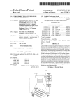
The gauge is a measure of the diameter of the wire; and #18 corresponds to a diameter of 1.2 x 10⁻³ m;
and #22 corresponds to a diameter of 6.4 x 10⁻⁴ m. The resistivity of iron is 9.7 x 10⁻⁸ Ωˑm; and the
value for copper is 1.72 x 10⁻⁸ Ωˑm.
1. Of the five wires, which one has the smallest resistance?
_______________
2. Which one of the wires carries the smallest current when they are connected to identical batteries?
_______________
3. What is the resistance of wire B? (Show work.) _______________
4. Wire B is connected to the terminals of a 1.5-V battery.
through the wire? _______________
33
What
magnitude
current
flows
Laboratory 4—Ohm’s Law and Resistivity
(Adapted from Jerry Wilson, Physics Laboratory Experiments, 4th Ed., pp. 353-357, © 1994 Houghton
Mifflin Company)
Purpose
The purpose of this experiment is to investigate the
resistivity of several different types of wires.
Introduction and Theory
Electric current is defined as the rate at which electric
charge flows through a surface,
The SI unit of current is the ampere (1 A = 1 C/s). The
direction of current flow is conventionally the direction of flow of positive charge. (This sign
convection is standard, although in most cases current is carried mainly by electrons. Electrons are
relatively free to move in solid conductors, and having less mass, electrons undergo a greater
acceleration then protons in a given electric field.)
Ohm’s law states that the potential difference V across a substance is proportional to the current I
flowing through it, V I . The proportionality is the resistance R; V = IR. The MKS unit for
resistance is the ohm (Ω). Thus, R = V/I.
The resistance of an electrical conductor depends on several factors, such as its physical shape, the type
of material it is made of, and the temperature. The resistance of a wire is directly proportional to its
length l and inversely proportional to its cross-sectional area, A:
l
A
R
An analogy for this is the flow of water through a pipe. The longer the pipe, the more resistance to
flow, but the larger the cross-sectional area of pipe, the greater the flow rate or the smaller the
resistance to flow. The material property of resistance is characterized by the resistivity ρ, and for a
given temperature:
R
l
A
Resistivity is independent of the shape of the conductor, and rearranging the previous expression gives
the equation for resistivity:
RA
, with units of Ω-m or Ω-cm
l
34
For a cylindrical wire, the cross-sectional area will be A = πD2/4. Thus, using R = V/I,
VD 2
4 I
V 2D I
D
I
V
35
Laboratory #4 Report Sheet: Ohm’s Law and Resistivity
Experimenters: _________________________
Course: __________________
_________________________
Day: ____________________
_________________________
_________________________
Objective
The objective of this experiment is to verify Ohm’s law and determine the resistivity of copper
and constantan wire.
Equipment
Ammeter (0-0.5 A)
Voltmeter (0-3V)
Rheostat (20 Ω)
Battery or power supply
Meter stick
Micrometers or Calipers
Conductor board or wires of various types, lengths
and diameters
1
1
1
1
1
1
1 (set)
Procedure
1. Set up the circuit as shown below, with one of the wires on the conductor board in the
circuit. Leave the rheostat set to the maximum resistance, and the power supply set to 0
or off, and have the instructor check the circuit before activating.
2. Turn up the DC volts of the power supply to 12V and adjust the rheostat until the current
in the circuit as indicated by the ammeter is 0.5 A. Record the meter values and the DC
volts back to 0 as soon as possible to prevent heating and temperature change.
3. Measure the length of the wire between the voltmeter connections and the diameter of the
wire.
a. Measure the voltage between each terminal to get five values (remember to
measure close to the spool and not at the terminals themselves)
b. Record L in cm and A in cm2 so we can compare with published values more
easily
c. The lengths are printed by each spool, and the thickness of each wire is
represented by the numbers 22 (for one value) and 28 (for a thinner value)
d. Thus, if you carefully measure the thickness of #1 and #2, you can assume that
the value of A for #1 is the same as that for #3 and #5; likewise for #2 and #4.
e. Thickness values are obtained by measuring as many consecutive turns as
possible, making sure they are one right next to another and not skewed…count
36
the number (N) of turns and measure the length along N turns, divide that value
by N to get the diameter of a single turn.
f. With the value for diameter, D, compute the cross-section area, A, with the
formula A = πD2/4
4. Find the percent error of the experimental values by comparing your values with the
accepted values listed below.
NOTE: For best results, the voltmeter should make contact with the resistance wire (R) about 5
cm in from the terminals, not at the terminals.
37
Data:
Substance
Aluminum
Brass
Constantan
Copper
German Silver (18% Ni)
Iron
Manganin
Mercury
Nichrome
Nickel
Silver
Tin
Resistivity, ρ (Ω-cm)
2.8 x 10⁻⁶
7 x 10⁻⁶
49 x 10-6
1.72 x 10⁻⁶
33 x 10-6
10 x 10-6
44 x 10-6
95.8 x 10⁻⁶
100 x 10-6
7.8 x 10⁻⁶
1.6 x 10⁻⁶
11.5 x 10⁻⁶
Ohm’s Law:
Wire: __4 (copper)__
V, Voltage
I, Current
Slope of V vs. I, R = ______________,
Average V = __________,
Wire: __5 (constantan)__
V, Voltage
I, Current
38
Average I = _________
Slope of V vs. I, R = ______________,
Average V = __________,
Average I = _________
Resistivity:
Wire
Diameter, D
Length, l
Voltage, V
Current, I
1 (copper)
2 (copper)
3 (copper)
4 (copper)
Ave=
Ave=
5 (constantan)
Ave=
Ave=
D = ______________; l = ______________; V = ______________; I = _____________
Data analysis:
Wire
ρcalc
ρknown
% error
% uncertainty
A, copper
B, copper
C, copper
D, copper
E, constantan
Summary:
Attach a typed Conclusion and Discussion section, addressing any questions your professor may
ask.
39
Pre-Laboratory Exercise #5: Series and Parallel Resistors
Name: _________________________
Course: __________________
Date: ____________________
Three resistors are placed in a circuit as shown. The potential difference between points A and B
is 30 V.
1. What is the equivalent resistance between points A and B?
_______________
2. Complete the following table for the potential difference and current across each of the
resistors
R (Ω)
ΔV (V)
10
30
60
40
I (A)
Laboratory 5—Series and Parallel Resistors
Purpose
The purpose of this lab is to learn how currents flow through simple linear series and parallel
circuits.
Introduction and Theory
Kirchoff’s rules state the conservation of energy and charge in an electrical circuit and can be
used to determine the distribution of current and voltage within an electrical circuit. Kirchoff’s
“loop rule” expresses conservation of energy.
“Loop rule”: The sum of the potential drops around any closed loop within a circuit is zero.
Simply put, start from any part of a circuit, go around a closed loop returning to the starting
point, and the potential must return to its starting value. Kirchoff’s “junction rule” expresses
conservation of charge.
“Junction rule”: The total current entering a junction must equal the total current leaving a
junction.
A junction is an intersection of conductors (wires). If the current into a junction were different
than the current leaving that junction, then charge would accumulate at the junction. This would
result in an electric field along the wires directed toward or away from the charge; the charge
would be accelerated away from the junction. In other word, because the charge carriers in a
conductor are free, an electric field cannot be sustained within a conductor. Therefore, charge
cannot accumulate at a junction.
41
These rules can be used to determine the equivalent resistance of combinations of resistors in
series and parallel. Consider a simple series combination as diagramed below.
Schematic for a Series Circuit is shown on the next page:
Vo = applied voltage
A = ammeter
V = voltmeter
R1 = resistor one
R2 = resistor two
When some number of resistors are arranged in a circuit hooked together in a series connection
as in the above diagram, the sum of the voltage drops across the separate resistors must equal the
applied voltage:
Vo = V1 + V2 +VA
Using Ohm’s law, V = IR, and the fact that the current in the circuit must everywhere be the
same, the voltage relation can be written
IReq IR1 IR2 IRA
where Req is the equivalent resistance of the circuit. Thus, the total resistance in the circuit is the
sum of the individual resistances. (Note that the ammeter has an internal resistance that needs to
be included in this experiment.)
Req Ri
(series)
i
When a set of resistors are arranged in parallel as in the diagram below, the total current into the
parallel part of the circuit is equal to the sum of the currents in each branch of the parallel circuit:
42
I o I1 I 2
Using Ohm’s law and the fact that the potential drop across each branch must be the same as the
applied voltage:
V
V
V
Req R1 R2
Thus, resistors in parallel are the same as the equivalent resistance:
1
1
Req
i Ri
(parallel)
Schematic for a Parallel Circuit:
A
Vo
I3
I2
I1
Vo = applied voltage
A = ammeter
V = voltmeter
R1 = resistor one
R2 = resistor two
The equivalent resistance of more complicated combinations of resistors can be determine by
determining the equivalent resistance of series and parallel portions of a circuit, then determining
the equivalent resistance of those combinations.
43
The following circuit can be examined for extra credit:
A
R3
Vo
I3
I1
I2
The regular procedure for this lab follows. In addition, the laboratory computers in NSCI 301 are
equipped with the Electronic Workbench / MultiSim utilities that are useful for supplementing
the electronics-based lab exercises with quality simulation. Documentation about MultiSim and
Electronics Workbench are available separately.
Optional Electronic Workbench / MultiSim Extension
Purpose or objective
To validate Ohm’s Law
Equipment
Multisim software and PC
Procedure
Series resistors:
Open the Multisim program. Click on place source this symbol
, which is in the upper left
corner of the program. Select POWER_SOURCES from the left column, then DC_SOURCES
from the right column, and then click ok. Go to anywhere on the page and left click. Then select
GROUND and click ok. Place the GROUND anywhere below the POWER_SOURCE. Go to the
drop down menu that has sources, click it, and then select basic. In the right column, select the
value resistor necessary, and then click ok. Click ok again to select another resistor until you get
the required number of resistors. Then click close to go to the circuit. Connect the circuit by
going to the tip of each component, left click, and then stretch the wire to the tip of the other
component then left click to attach the wire to the other component. Repeat this until the circuit
is complete. See figure 1 below.
44
Figure 1: Resistors in series.
Now, we want to confirm Ohm’s Law by measuring the voltage drop across the resistors. Let’s
measure the voltage drop across resistor R2 and the current between resistors R2 and R3. Click
on place indicator this symbol , which is along the same row as the place sources symbol.
Click on VOLTMETER in the left column and click on VOLTMETER_H in the right column,
then click ok. Then click on AMMETER in the left column and click on AMMETER_H in the
right column, click ok. Then click close. Connect wires from the VOLTMETER to the wire and
from the AMMETER to the wire. Click on the wire below the AMMETER and click delete. The
circuit should look like figure 2 below.
Figure 2: Circuit with VOLTMETER and AMMETER
Click the run button . Wait for a few seconds then when you see the measurements on the
VOLTMETER and AMMETER, click stop . Record your measurements.
45
Parallel resistors
Click new . Create the schematic as shown in the figure 3 (next page). Click run and record
your measurements.
Figure 3: Resistors in parallel
Results
Series:
Voltage
Parallel:
Voltage
Current
Current
Safety Reminder
Caution: Be very careful not to short-circuit the power supply. With too little resistance in a
circuit, the current can exceed 1 A. The power supplies have a fuse that breaks the circuit if the
current exceeds 1 A.
46
Laboratory #5 Report Sheet: Series and Parallel Resistors
Experimenters: _________________________
Course: __________________
_________________________
Date: ____________________
_________________________
_________________________
Objective:
The objective of this experiment is to determine the equivalent circuit resistance of simple
combinations of resistors in series and parallel.
Equipment
Ammeter (0-0.5 A)
Voltmeter (0-10V)
Ohmmeter or multimeter
Rheostats (44 or 177 Ω) or resistors
Power supply
Connecting wires
3
1
1
3
1
as needed
Procedure
We will determine the equivalent resistance of the circuits below by four methods:
(1)
(2)
(3)
(4)
Direct ohmmeter measurement of Req,
Theoretica1 Req using individual ohmmeter measurements of R,
Req from using ohm’s law for circuit,
Theoretical Req from individual Ohm’s law measurements of R.
1. Measure the resistance of each of the resistors and ammeters to be used below. (Note: refer to
the lab write-up for schematics for each of the following circuits)
Series Circuit:
2. Set up the circuit shown above for two resistors in series. For a fixed setting for the power
supply:
3. Measure the current in the circuit and the voltage drops across each of the resistors and the
ammeter.
4. Measure the closed circuit voltage across the battery.
5. Remove the wires from the battery and measure the total resistance, Req, of the circuit by
placing the ohmmeter leads on these two wires. (This is often called the open circuit
resistance.)
Parallel Circuit:
47
6. Set up the circuit shown above for two resistors in parallel. For a fixed setting of the power
supply:
7. Measure the total current in the circuit and the current in each branch.
8. Measure the voltage drop across each resistor and ammeter. (To avoid further complexity,
call R1 (R2) the series combination of the resistor and ammeter in that branch.)
9. Measure the open circuit resistance, Req.
Extra Credit Circuit:
10. Set up the circuit shown above for three resistors in series and parallel. For a fixed setting of
the power supply:
11. Measure the total current in the circuit and the current in each branch.
12. Measure the voltage drop across each resistor and ammeter.
13. Measure the open circuit resistance, Req.
48
Data
Series Combination
Ohmmeter measurements:
Parallel Combination
Extra Credit
(incl. ammeter)
(incl. ammeter)
R1 R1
R2 R2
R3 R3
NA
NA
NA
NA
R A R A
Req Req
Voltage measurements:
V1 V1
V2 V2
V3 V3
V A V A
Vo Vo
Current measurements:
I o I o
I1 I1
NA
I 2 I 2
NA
Data Analysis
Series Circuit
Equivalent resistance from ohmmeter:
Req R1 R2 R A = _______________
Req R1 R2 RA = _______________
Measured Req Req = ______________
Resistance from Ohm’s law:
49
V1 I o
_______________
V
I
o
1
R1
V1
____________________
Io
R1 R1
R2
V2
____________________
Io
R2 R2
RA
VA
____________________
Io
R A R A
Req
Vo
____________________
Io
Req Req
Req R1 R2 R A = _______________
V2 I o
_______________
V
I
o
2
V A I o
_______________
V
I
o
A
Vo I o
Io
Vo
_______________
Req R1 R2 RA = _______________
Parallel Circuit (Include RA in series if needed.)
Resistance from ohmmeter:
Req
R1 R2
= ___________
R1 R2
R1 R2 R1 R2
= ___________
R2
R1 R2
R1
Req Req
Measured Req Req = ______________
Resistance from Ohm’s law:
V1 I 1
_______________
I 1
V1
R1
V1
____________________
I1
R1 R1
R2
V2
____________________
I2
R2 R2
Req
Vo
____________________
Io
Req Req
Req
R1 R2
= ___________
R1 R2
R1 R2 R1 R2
= ___________
R
R
R
R
2
1
2
1
V2 I 2
_______________
I 2
V2
Vo I o
_______________
I o
Vo
Req Req
50
Extra Credit (Include RA in series if needed.)
Resistance from ohmmeter:
Req R3
R1 R2
= _________
R1 R2
R1 R2 R1 R2
= ________
R2
R1 R2
R1
Req R3 Req
Measured Req Req = ______________
Resistance from Ohm’s law:
V1 I 1
_______________
I 1
V1
R1
V1
____________________
I1
R1 R1
R2
V2
____________________
I2
R2 R2
V2 I 2
_______________
I 2
V2
V3 I o
Io
V3
_______________
R R R1 R2
RR
= ________
Req R3 Req 1 2
Req R3 1 2 = _________
R2
R1 R2
R1 R2
R1
V I
V
Req Req o o _______________
Req o ____________________
Io
Io
Vo
R3
V3
____________________
Io
R3 R3
Summary:
For each circuit, compare Req found by the four methods. Attach a typed Conclusion
section and a Discussion section.
Optional extension may be done alongside with or after the main experiment. This is the
Electronic Workbench exercise provided in the first part of the lab write up.
Extra Credit (up to 3 pts.) can be obtained for the equivalent-resistance analysis of the
extra-credit circuit.
51
Pre-Laboratory Exercise #6: RC Circuits
Name: _________________________
Course: __________________
Date: ____________________
1. In a circuit such as the one in Figure 1 (on back) with the capacitor initially uncharged, the
switch S is thrown to position A at t = 0. The charge on the capacitor is
(a)
(b)
(c)
(d)
initially zero and finally Cε.
constant at a value of Cε.
initially Cε and finally zero.
always less than Cε.
2. In a circuit such as the one in Figure 1 with the capacitor initially uncharged, the switch S is
thrown to position A at t = 0. The current in the circuit is
(a)
(b)
(c)
(d)
initially zero and finally ε/R.
constant at a value of ε/R..
equal to ε/R..
initially ε/R and finally zero.
3. In a circuit such as the one in Figure 2 the switch S is first closed to charge the capacitor, and
t
then it is opened at t = 0. The expression V = εe− /RC gives the value of
(a)
(b)
(c)
(d)
the voltage on the capacitor but not the voltmeter.
the voltage on the voltmeter but not the capacitor.
both the voltage on the capacitor and the voltmeter, which are the same.
the charge on the capacitor.
4. If a 5.00 μF capacitor and a 3.50 MΩ resistor form a series RC circuit, what is the RC time
constant? (Show work.) ____________________
5. Assume that a 10.0 μF capacitor, a battery of emf ε = 12.0 V, and a voltmeter of 10.0 MΩ
impedence are used in a circuit such as that in Figure 2. The switch S is first closed, and then the
switch is opened. What is the reading on the voltmeter 35.0 s after the switch is opened? (Show
work.) ____________________
52
53
Laboratory 6—RC Circuits
Purpose
The purpose of this activity is study
currents and voltages in RC circuits. We
will use a Resistor and a Capacitor to
study the capacitor’s transient response
as it is charged then discharged.
NOTE: If you need to familiarize
yourself with the oscilloscope, before
you start on this experiment, work
through the exercise in Appendix A
designed to familiarize you with this
instrument. If you are doing this
experiment using the computer and
PASCO’s DataStudio, no such review is
necessary (a write up for this version of the lab is forthcoming).
Introduction and Theory
A Resistive-Capacitance, or RC circuit is an electronic circuit that is driven by a voltage or
current source such as a battery or power supply. The simplest form of such a circuit is the “First
Order” RC circuit consisting of one resistor and one capacitor. Along with the inductor (L) the
resistor and the capacitor make up three basic linear analog components which, when put
together in various combinations, exhibit behavior that is fundamental to much of analog
electronics and, thus, have important applications. They are commonly used as passive filters.
Two fundamental types of passive filters are the high-pass filter and the low-pass filter. The
high-pass filter presents less attenuation to high-frequency signals than low-frequency signals by
passing a signal through a capacitor or a path to ground through an inductor. The low-pass filter
presents less attenuation to low-frequency signals than high frequency signals by passing the
signal through an inductor or by allowing a capacitor to provide a path to ground. These are two
types of electronic circuits that allow wanted frequencies to pass through while blocking
unwanted ones.
If a capacitor (C) is connected to a voltage source (V) charge will acquire on the plates. As the
charge on the plates increases it becomes more difficult to add additional charge because of the
increasing Coulomb force. This continues until the voltage across the plates equals that of the
voltage source. At any time (t), the charge (Q) on the capacitor plates is given by
Q CV
The rate at which the capacitor charges and discharges is dependent on the capacitor and resistor
in the circuit. An important term in charging and discharging a capacitor is the RC time constant
54
RC
Referring to the circuit shown in Figure 1, when the switch is in position A, the capacitor will
charge. When charging a capacitor with a DC source, Vo, the voltage (Vc) and charge Q will
increase over time. The voltage is characterized by the equation
VC (t ) Vo (1 e t / RC ) Vo (1 e t / )
If t = RC = then the equation reduces to
1
VC (t ) Vo (1 e t / ) Vo (1 ) 0.63Vo
e
So, the capacitor is 63% charged at t = RC. The time to fully charge the capacitor will be
infinite. The capacitor will be 99.3% charged after five time constants.
When the switch in Figure 1 is at position B, the capacitor will discharge its energy through the
resistor. When discharging a capacitor the voltage (Vc) and charge Q will decrease over time.
The voltage is characterized by the equation:
VC (t ) Vo e t / RC Vo e t /
If t = RC = then the equation reduces to:
VC (t ) Vo e t / Vo
1
0.37Vo
e
So, the capacitor is 37% discharged at t = RC.
Since Q = C Vc, the amount of charge on capacitor while charging and discharging it is given by
Charging:
Q(t ) Qo (1 e t / RC ) Qo (1 e t / )
55
Discharging: Q(t ) Qo e t / RC Qo e t /
For charging an initially uncharged capacitor or discharging an initially fully charged capacitor,
the circuit current varies as
I I o e t /
56
Vo t /
e
R
Laboratory #6 Report Sheet: RC Circuits
Experimenters: _____________________
Course: __________________
_____________________
Date: ____________________
_____________________
_____________________
Objective
The objective of this experiment is to use an RC circuit and the rate at which a capacitor charges
and discharges, namely, the RC time constant, to determine its capacitance.
Equipment
DC Power Supply
1
Resistor Box
1
Capacitor (100F)
1
2-Position Switch
1 (optional)
Data Studio w/ Voltage Sensor, 1
Lead Wires
5
Alligator Clips
5
Procedure
1. Set the resistor box for a time constant RC ≈ 1 s. (e.g., if C = 100 F, then R = 10 kΩ.)
2. Short the capacitor by connecting the leads together to ensure that it is not charged.
3. Connect the circuit shown in Figure 1 with the switch at position B.
4. Open Data Studio and connect to the voltage sensor. Setting the sampling rate to 100 Hz will
permit measurements of time constants greater than 0.1 s.
5. Connect the Data Studio voltage sensor across the capacitor.
6. Turn on the power supply and set the voltage not to exceed 8 V. (Do not saturate the power
supply voltage.)
7. Start Data Studio to graph Vc vs. t.
8. Move the switch to position A to charge the capacitor.
9. When the voltage plateaus (Vc ≈ Vo), move the switch to position A to discharge the capacitor.
10. Stop Data Studio when the capacitor is nearly fully discharged (Vc ≈ 0), and you are satisfied
with the resulting curves. (If not satisfied, repeat steps 8 and 9 until you are, or start a new data
set by repeating steps 7−10.
11. Highlight the voltage rise (charging) and fit with an “inverse exponential” fit to obtain the
time constant. Print the fitted data noting the values used for the resistance and capacitance on
the plot.
12. Highlight the voltage decline (discharging) and fit with a “natural exponential” fit to obtain
the time constant. Print the fitted data noting the values used for the resistance and capacitance
on the plot.
57
13. Change the value of the resistance on the resistance box by a factor of 2 to 10, and repeat the
experimental steps 7−12.
Data and Data Analysis
Experiment 1
Vo = _______________,
R = _______________,
C = _______________
Theoretical τ = RC = _______________
Experimental τ (charging) = ____________,
Experimental τ (discharging) = ____________
(Plots attached.)
Experiment 2
Vo = _______________,
R = _______________,
C = _______________
Theoretical τ = RC = _______________
Experimental τ (charging) = ____________,
Experimental τ (discharging) = ____________
(Plots attached.)
Conclusion
Attach a typed Conclusion and Discussion section.
Questions:
For questions 1 and 2 below, assume an RC circuit as above with Vo = 10 V, C = 100 F, and R
= 10 kΩ. (Show your work.)
1. Assuming the capacitor is initially uncharged, what is the value of the voltage across the
capacitor after 5 time constants? ______________
2. With VC (t ) Vo e t / RC Vo e t / , it mathematically takes an infinite time for the capacitor in an
RC circuit to discharge completely. Practically, how many time constants does it take for the
capacitor to discharge to less than 1% of its initial voltage? _______________
3. What is the time constant of the circuit shown above? _______________
58
Pre-Laboratory Exercise #7: Magnetic Force
Name: _________________________
Course: __________________
Date: ____________________
1. An electron traveling horizontally enters a region where a uniform magnetic field is directed
into the plane of the paper as shown. Which one of the following phrases most accurately
describes the motion of the electron once it has entered the field?
(a) upward and parabolic
(b) upward and circular
(c) downward and circular
(d) upward, along a straight line
(e) downward and parabolic
2. An electron is moving with a speed of 3.5 × 10⁵ m/s when it encounters a magnetic field of
0.60 T. The direction of the magnetic field makes an angle of 60.0° with respect to the velocity
of the electron. The magnitude of the magnetic force on the electron is ________________.
(Show your work.)
3. A 0.150-m wire oriented horizontally between the poles of an electromagnet carries a direct
current of 12.5 A. The angle between the direction of the current and that of the magnetic field
is 25.0°. If the magnetic field strength is 0.625 T, what is the magnitude and direction of the
magnetic force on the wire between the poles? ______________________ (Show your work.)
NOTE: The Magnetic Force Lab, if it is performed, will be done using the Instruction
Manual and Experiment Guide for the PASCO Scientific Model SF-8607 and SF-8608
Basic Current Balance and Current Balance Accessory. Hard copies are available in the
drawers where lab forms are kept, and a soft copy version is appended as an appendix to
this document.
59
Pre-Laboratory Exercise #8: Magnetic Induction
Name: _________________________
Course: __________________
Date: ____________________
1. The magnetic flux through a surface is defined as Φ = BA
magnetic flux (a) maximum and (b) minimum?
. At what angle is the
(a) __________
(b) __________
2. A 2-T uniform magnetic field makes an angle of
with the z axis. The magnetic flux
2
through a 3 m portion of the x-y plane is________________. Show your work.
3. Faraday’s law states that an induced emf is proportional to the
(a)
(b)
(c)
(d)
rate of change of magnetic field.
rate of change of electric field.
rate of change of magnetic flux.
rate of change of electric flux.
4. In an experiment, two coaxial coils are used to investigate induction. A sinusoidal current is
passed through the first coil. The induced emf in the second coil does not depend on the
(a)
(b)
(c)
(d)
(e)
frequency of the current.
number of turns in coil 2.
area of coil 2.
resistance of coil 2.
amplitude of the current in coil 1.
60
Laboratory 8—Magnetic Induction
Purpose
The purpose of this experiment is to understand how changing magnetic fields can produce
electric currents. In doing so, we examine Lenz's Law and Faraday's Law.
Introduction and Theory
Magnetic flux is defined as the product of magnetic field lines and the area through which they
pass. Of importance is that the total magnetic flux through a closed surface is zero. This implies
that monopoles do not exist. The magnetic flux is dependent on the strength of the magnetic
field, the size of the area through which they pass and the angle between the normal of the area
and the magnetic field. We will investigate the dependence of flux on these variables and how a
changing flux can induce currents in other coils.
One practical use for inductance is to detect the presence of cars at a stoplight. An inductive loop
is a coil of wire that winds a certain number of turns. This coil is embedded in the road’s surface
and works by detecting a change of inductance. This change comes about when a large steel
object, the car, is placed within the inductor’s magnetic field and that changes the inductance,
which is detected by a meter, which then sends a command to the light to switch from red to
green after a short interval of time.
When electric current first starts flowing in a coil, the coil’s tendency is to build up a magnetic
field. While the field is building, the coil inhibits the flow of current. Once the magnetic field is
built up, the current flows normally through the wire. When the switch is opened, and the circuit
is broken, the magnetic field around the coil maintains an electric current until the magnetic field
collapses. The inductor has a characteristic called capacity which is influenced by two factors:
The number of coils
The material that the coils are wrapped around (the core)
Putting iron in the core of an inductor gives it much more inductance than air or any other nonmagnetic core would. There are devices that can measure the inductance of a coil, and the
standard unit of measure is the Henry.
Magnetic flux is defined as the product of the magnetic field and the area through which they
pass. The magnetic flux is dependent on the strength of the magnetic field, the size of the area
through which they pass and the angle between the normal of the area and the magnetic field.
Recall that the electric flux through any closed surface is proportional to the electric charge
enclosed by the surface. There are no magnetic charges (monopoles), and the magnetic flux
through any closed surface is zero. However, a changing magnetic flux will produce an emf in a
conductor and cause a current to flow.
Magnetic flux through a surface is defined as BA cos , where B is the magnetic field in
tesla, A the area in m2 and θ the angle between the area normal and the magnetic field. When θ
is 900 the magnetic field is in the plane of the surface and Φ = 0. When θ= 00 or 1800 the
magnetic field is perpendicular to the surface and Φ is a maximum value BA.
61
Faraday’s law states a changing magnetic field induces an electric field, this is summarized in the
following equation,
, where ε is the electromotive force, and Φ is the magnetic flux. It
t
states, if we have a magnetic flux which changes in time, it induces an emf. If that emf is
induced in a material capable of carrying a current, a current will result. The sense of the current
will be such that it produces a magnetic field that opposes the changing magnetic flux. This is
Lenz’s law:
The induced current in a loop is in the direction that creates a magnetic field that
opposes the change in magnetic flux through the area enclosed by the loop.
Again, Faraday’s law of induction is
N 2
( BA cos )
B
N2
N 2 A cos
t
t
t
where we assume a secondary coil (coil 2) of N2 turns. To generate our magnetic field we shall
use a 200-turn Helmholtz coil, coil 1. Along the axis perpendicular to the loop the magnitude of
the magnetic field is
B
o N1 I 1 R1 2
2( x 2 R1 ) 3 / 2
2
where o 4 10 7 TAm is the permeability of free space, I is the current, N is the number turns
and R is the radius of the coil, and x is the distance perpendicular along the coil axis. A signal
generator will provide a sinusoidal current to the primary coil to produce B. Hence,
B Bo sin(2ft ) , where Bo
o N1 I 1 max R1 2
2( x 2 R1 ) 3 / 2
2
And…
N 2 A cos
B
2fN 2 Bo A cos cos(2ft )
t
62
Laboratory #8 Report Sheet: Magnetic Induction
Experimenters: _________________________
Course: __________________
_________________________
Date: ____________________
_________________________
_________________________
Purpose
The purpose of this experiment is to examine Faraday’s law of induction which states that a
changing magnetic flux produces an emf and electric current in a conductor.
Equipment
Oscilloscope
Function Generator
Helmholtz Coils
Coaxial Cables
1
1
1 pair, with base
1 set
Procedure
Connect the experiment as shown below…
Coil 2
Coil 1
Oscilloscope
Signal Generator
Changing
Magnetic Field
63
Data
Calculate the magnetic field in coil 1 and coil 2 when it is 10 cm from coil 1 and both coils are
parallel to each other. Use Ohm’s law, V = IR to obtain the current. (Show work.)
V1 = ________________; R1 = _______________; I1 = _______________
Bcalculated_1 = ________________ tesla
Bcalculated_2 = ________________ tesla
Complete Table 1 Below (For ease, you may record peak-to-peak voltage.)
Angle
degrees
0
Distance
between
Coils
10 cm
Frequency
Coil 1
Hz
200 Hz
10
10 cm
200 Hz
20
10 cm
200 Hz
30
10 cm
200 Hz
40
10 cm
200 Hz
50
10 cm
200 Hz
60
10 cm
200 Hz
70
10 cm
200 Hz
80
10 cm
200 Hz
90
10 cm
200 Hz
100
10 cm
200 Hz
110
10 cm
200 Hz
120
10 cm
200 Hz
130
10 cm
200 Hz
140
10 cm
200 Hz
150
10 cm
200 Hz
160
10 cm
200 Hz
170
10 cm
200 Hz
180
10 cm
200 Hz
Voltage 1
Volts
Make a graph of the induced voltage (V2) versus angle
64
Voltage 2
Volts
V2/V1
a. What is the shape of the induced voltage in coil 2 versus angle?
b. Is this what you expected and why?
c. What is observed of the frequency in coil 2? How does it compare to the frequency in
coil 1? What does this tell you?
d. At 0o what is the peak voltage in coil 2? What did you expect for this value?
Complete Table 2 Below (For ease, you may record peak-to-peak voltage.)
Angle
degrees
0
Distance
between
Coils
3cm
Frequency
Coil 1
Hz
150
0
4 cm
150
0
6 cm
150
0
8 cm
150
0
10 cm
150
0
12 cm
150
0
14 cm
150
0
16 cm
150
0
18 cm
150
0
20 cm
150
Voltage 1
Volts
Make a graph of the induced voltage versus distance
65
Voltage 2
Volts
V2/V1
a. What is the shape of the induced voltage in coil 2 versus distance?
b. Is this what you expected and why?
c. What did you observe about the emf values based upon the distance between the coils?
d. What is observed of the frequency in coil 2? How does it compare to the frequency in
coil 1? What does this tell you?
Things to Consider
1. Do you think it is possible to measure the earth’s magnetic field in a given direction by
looking at the induced emf in a coil? If so, how would you construct the experiment and
determine its value?
2. Can you use coil 2 to determine the presence of other signals in the vicinity? How would
you demonstrate this and which frequencies if any did you find?
3. How do you think the number of turns affects the outcome of the experiment?
66
Pre-Laboratory Exercise #9: RLC Circuits
Name: _________________________
Course: __________________
Date: ____________________
A
Consider the RLC circuit shown above with a peak voltage of 240 V, f = 60 Hz, R = 100 kΩ,
L = 0.5 mH, C = 200 µF. (Show your work.)
1. What is the impedance of the circuit? _________________
2. What is the value of the current read by the ammeter? _______________
3. What is the (linear) resonant frequency of the circuit? _______________
67
Laboratory 9—RLC Circuits
Purpose
The purpose of this experiment is to study currents and voltages in RLC circuits. We will
measure the response of the voltage across a resistor (Vr) as a function of a voltage applied at
different frequencies.
Introduction & Theory
When an inductor L, a resistor R and a capacitor C are connected in series, the alternating current
I present in the circuit depends on the frequency of the driving voltage E. This type of circuit is
used extensively in electronic devices, particularly radios and televisions.
These circuits are used in a number of electronics applications including the tuning of analog
radios and televisions. Adjustable tuning is usually achieved by using a parallel plate variable
capacitor which enables the value of C to be changed, which enables the receiver to tune to
stations of different frequencies. The inductor comes with an adjustable core which enables the
inductance, L, to be changed. The core is made of a high permeability material that effectively
increases inductance and is threaded so that it can be screwed in or out of the inductor winding as
needed.
Filters are another common use of RLC circuits. In a filtering application, the resistor R becomes
the load that the filter is working into. The damping factor value is selected based on the desired
bandwidth of the filter. A wider bandwidth uses a larger damping factor and vice versa. The
three components of the circuit give three degrees of freedom to the designer of the circuit to
enable the desired outcome to be met. Two of the components are required to set the bandwidth
and the resonant frequency; the third can be adjusted in such a way so as to scale each of the
three components to convenient values. In another setting, R may be predetermined by the
circuitry within which this circuit is found and which will use this last degree of freedom.
Other common uses of RLC circuits include the use of the circuit as an oscillator whereby the
attenuation (or damping factor) is made as small as possible. This can be adjusted by making the
R be as small as possible for series circuits and as large as possible for parallel circuits. Other
uses also include making the circuit a voltage multiplier or a pulse discharge circuit.
An important property in RLC circuits is resonance, which is the ability of the circuit to resonate
at a specific frequency, called the resonant frequency. Resonance in the circuit happens because
energy is stored in two different ways: as an electric field as the capacitor is charged, and as a
magnetic field as the current flows through the inductor. Energy can be transferred from one to
the other and back again in an oscillatory mode, much like the mass at the end of a spring
oscillates back and forth between one extreme and the other. The mathematics describing both
are identical in form. Whereas friction in the spring-mass system will eventually bring the
system to a halt, the resistance in the RLC circuit will diminish the oscillation over time. Like a
vibrator that can keep the mass on a spring oscillating indefinitely, the driving AC power source
will keep the circuit resonating indefinitely.
68
The resonant frequency is defined as the frequency at which the impedance of the circuit is at a
minimum. In the series LRC circuit that we will be studying, the impedance reaches a minimum
when resonance is achieved (in parallel LRC circuits this happens when the impedance reaches a
maximum). The resonant frequency is reached because the inductor and capacitor are equal but
of opposite sign, so they cancel out.
The AC current of a RLC circuit connected in series depends on the voltage and impedance.
V
I
Z
Impedance is the AC circuit equivalent of resistance. This describes not only the amplitude of
voltages and currents but also the relative phases. The impedance is defined mathematically as:
:
Z
X
X C R
2
L
2
1
, and R is the
C
resistance and the angular frequency is 2f where f is the linear frequency. The current
will have a maximum value at resonance when X L X C this condition defines the resonant
Where the inductive reactance is, X L L the capacitance reactance is X L
1
. For this condition the impedance Z = R and has a minimum value,
LC
which results in the current having a maximum value.
frequency at
res
Note: This lab has several variations which are included below. The standard report sheet with
its procedure is also included. The professor may decide to do one or the other (or a combination
of both). In addition an electronic workbench activity is added.
Suggested Procedure
1.
Set up the circuit as shown below. The function generator will apply the voltage to the
circuit at different frequencies. The oscilloscope will measure the voltage across the
resistor. Record the data in the table
2.
Plot a graph of Vr vs. linear frequency (f)
3.
Determine the inductive reactance, Capacitive reactance, impedance and amplitude of
the current through the resistor and plot XL vs. frequency (f), XC vs. f, and Z vs. f.
4.
Refer to the “Analyzing the data” section on the image below.
69
70
Results
Complete Table 1:
Linear
Frequency
Vr (V)
X L 2fL (Ω)
XC
1
(Ω)
2fC
71
Z (Ω)
I V R (Ω)
Z
Complete Table 2 Below:
Parameter Name
Parameter Value
Inductance
Resistance
Capacitance
Resonant Frequency (linear)
Resonant Angular Frequency
Theoretical Resonant Angular Frequency
Conclusions & Questions
1.
How does the measured value for the resonant angular frequency compare to the
theoretical value for the resonant angular frequency?
2.
Is the plot of impedance current versus frequency symmetrical about the resonant
frequency? Explain.
At resonance, the reactances of the inductor and the capacitor cancel each other out so that the
impedance (Z) is equal to just the resistance R. Calculate the resistance of the circuit by using the
amplitude of the current at resonance in the equation R = V/I. Is the resistance equal to that used
in the circuit? Why or why not?
Optional Electronic Workbench / MultiSim Extension
Purpose
The purpose of this activity is study currents and voltages in RLC circuits. We will measure the
response of the voltage across a resistor (Vr) as a function of a voltage applied at different
frequencies using Multisim.
Equipment
Multisim software
72
Procedure
Open the Multisim program. Click on PLACE, then click on COMPONENT. Click on the drop
down bar below GROUP and select BASIC. Select RESISTOR and under COMPONENT, select
the value resistor then click ok. Select CAPACITOR, select the value, then click ok. Select
INDUCTOR, select the value, then click ok. Click on the drop down bar below GROUP, select
SOURCES, then POWER_SOURCES, then GROUND, then click on ok. Go to the same drop
down bar, select INDICATORS, then select AMMETER, the select AMMETER_H then click
ok. Then close the SELECT A COMPONENT tab.
Go to the right side of the program. Run the mouse over the icons and select FUNCTION
GENERATOR
. Drag it closer to the other components and the left click. Go back to the
right side of the program and select OSCILLOSCOPE
. Drag it closer to the other
components and left click. Click on the edge of the components and use the wire to connect
them. The circuit should look like figure 1 below. Ensure that the positive terminal of the
function generator goes to the positive terminal of the ammeter. Check the schematic in the
figure 1 below to ensure that the terminal match your schematic.
Double click on the oscilloscope. Then click run
or
. Then click stop
or
. Pull
the green vertical line that is on the left of the graph to the crest of the sine wave on the graph (It
will change color to yellow). Then pull the red vertical line to the trough (it will change to blue)
and record your results given by the yellow vertical line. Your results should look like figure 2
below.
Double click on the function generator and change the frequency. Run and stop the experiment
and record your results.
Figure 1: RLC Circuit.
73
Figure 2: Results should look like this
Results
Conclusion
Please include a conclusion statement with your write-up.
74
Laboratory #9 Report Sheet: RLC Circuits
Experimenters: _________________________
Course: __________________
_________________________
Date: ____________________
_________________________
_________________________
Purpose
The purpose of this activity is to study the currents and voltages. We will measure the response
of the voltage across a resistor (Vr) as a function of a voltage applied at different frequencies.
Introduction and Theory
Schematic
f = adjustable frequency
ω=2 f
V= voltage
I = current
Overall resistance:
Z
V
V
1
2
I , Z R 2 X L X C where X L * L and X C
I
Z
*C
75
The smallest Z , occurs when X L = X C ; Resonance condition… 0 * L
0
1
1
, f0
3600Hz
2 L * C
L *C
R ___
L = 1.92mH = 1.92*103 H
C 1 F 1*106 F
(a) Calculate f 0 (theoretically)
(b) Determine experimentally the value of f 0 (experimentally).
Power or amplitude
Pavg
2
V2
1
1
1
2
2
R or rms I rms
I 0 , Vrms
V0
amplitude I rms
2
R
2
2
1 1
Vpp
22
I rms R
Vrms
Vrms
Oscilloscope reads V0, AC meter reads I rms , Vrms
76
1
1
0 2
0 * C
L *C
Q or Quality of circuit
2 f 0 L
R
L
Q 0
R
Q
Equipment
The following components can be used as is or
substituted by PASCO’s AC/DC Electronics Laboratory
System
Oscilloscope
1
Function Generator
1
Inductors
2
Capacitor
1
Resistor
1
Procedure
Setup the circuit as shown below. The function generator will apply the voltage to the circuit at
different frequencies. The oscilloscope will measure the voltage across the resistor. Record the
data in the table.
Plot the graph of Vr vs. linear frequency (f)
Determine the inductive reactance, capacitive reactance, impedance and amplitude of the current
through the resistor and plot XL, XC and Z vs frequency (f)
Refer to the “Analyzing the data” section on the image below.
77
RLC Circuit
Analyzing the data
From the graph find the linear resonant frequency, fres
Using the resonant frequency fres, calculate the resonant angular frequency, ωres and record the
value in the Table 2
Calculate the theoretical resonant angular frequency using the values of the inductance and
capacitance.
Compare the theoretical resonant frequency to your measured resonant frequency
78
Results
Complete Table 2 Below:
ITEM
VALUE
Inductance
Resistance
Capacitance
Resonant Frequency (linear)
Resonant Angular Frequency
Theoretical Resonant Angular
Frequency
79
Conclusion & Questions
How does the measured value for the resonant angular frequency compare to the theoretical
value for the resonant angular frequency?
Is the plot of impedance current versus frequency symmetrical about the resonant frequency?
Explain.
At resonance, the reactances of the inductor and the capacitor cancel each other out so that the
impedance (Z) is equal to just the resistance R. Calculate the resistance of the circuit by using the
amplitude of the current at resonance in the equation R=V/I. Is the resistance equal to the used in
the circuit? Why not?
80
Pre-Laboratory Exercise #10: Reflection and Refraction of Laser
Light
Name: _________________________
Course: __________________
Date: ____________________
1. Light refracts when it travels from one medium to another. Explain why? What principle
explains this behavior?
2. Given that the speed of light in a given medium is 2.3 × 10⁸ m/s. Find the index of refraction,
n, for that medium.
For questions 3 - 5, consider the figure given above in which light
(f1 = 5.5 × 10¹⁴ Hz) travels from medium 1 to medium 2. The index
of refraction for medium one and two are 1.2 and 1.6, respectively.
The angle of incidence θ1 is 68°.
3. What is the frequency in medium 2?
4. What is the velocity of light in medium 2?
5. Find the angle of refraction, θ2? (Show work.)
81
Laboratory 10—Reflection and Refraction of Laser Light
Purpose
The purpose of this laboratory exercise is to study the nature of reflection and refraction of laser
light and find the index of refraction of the material used.
Introduction
When a light beam falls on a surface, both reflection from the surface and refraction into the
substance occurs. Refraction is the bending of light as it passes from one substance to another.
As light passes from a less dense to a more dense material it bends towards the perpendicular to
the plane of the surface of the material. Conversely, light entering a less dense material will bend
away from the perpendicular to the plane of the surface. The amount of bending which occurs
depends both on the wavelength of the light and the type of material through which the light is
propagating. A property of the material related to the amount of refractive bending is called the
index of refraction of the material. The index of refraction of a material is usually quoted with
respect to vacuum, where the vacuum is defined to have an index of refraction of one. The index
of refraction of air is almost that of a vacuum, so light traveling in air can be considered to be in
a vacuum. (This is a good approximation to an accuracy of three significant figures).
On the next page is a table of the index of refraction for a number of everyday items. This list is
composed from lists that appear on several websites such as http://hyperphysics.phyastr.gsu.edu/hbase/tables/indrf.html
and
the
interactive
website
http://interactagram.com/physics/optics/refraction/, which provides a fairly detailed description
of the phenomenon of refraction.
82
Index of Refraction of Selected Materials
Material
Index
Vacuum
1.00000
Water (gas)
1.000261
Argon
1.000281
Air at STP
1.0002926
Nitrogen (liq)
1.2053
Alcohol
1.329
Ice
1.309
Water 100'C
1.31819
Methanol
1.329
Water 35'C (Room temp)
1.33157
Water 20'C
1.33335
Teflon
1.35
Acetone
1.36
Ethanol
1.36
Ethyl Alcohol
1.36
Sugar solution (30%)
1.38
Fluorite
1.433
Aluminum
1.44
Opal
1.450
Quartz, Fused
1.45843
Plastic
1.460
Turpentine
1.472
Glycerine
1.473
Onyx
1.486
Glass, Albite
1.4890
Sugar solution (80%)
1.49
Ulexite
1.490
Plexiglas
1.50
Dolomite
1.503
Gaylussite
1.517
Glass
1.51714
Rubber, Natural
1.5191
Crown glasses
1.52-1.62
Typical crown glass
1.52
Nylon
1.53
Thomsonite
1.530
Sodium chloride
1.54
Material
Rock Salt
Sodium Chloride
Quartz
Amethyst
Amber
Polystyrene
Emerald, Synth flux
Emerald, Synth hydro
Flint glasses
Glass, Flint, Light
Styrofoam
Topaz, Blue
Turquoise
Mercury (liquid)
Topaz
Topaz, Pink
Topaz, Yellow
Topaz, White
Glass, Flint, Medium
Carbon disulfide
Asphalt
Glass, Flint, Heavy
Glass, Flint, Dense
Olivine
Methylene iodide
Ruby
Sapphire
Rare earth flint
Glass, Flint, Lanthanum
Pyrite
Lanthanum flint
Glass, Flint, Heaviest
Sulphur
Crystal
Arsenic trisulfide glass
Zirconia, Cubic
Diamond
Theory
The defining equation for the index of refraction between any two materials is:
nα sin α = nβ sin β
83
Index
1.544
1.544
1.544
1.544
1.546
1.55-1.59
1.561
1.568
1.57-1.75
1.58038
1.595
1.610
1.610
1.62
1.620
1.620
1.620
1.630
1.62725
1.63
1.635
1.65548
1.66
1.670
1.74
1.760
1.760 – 1.77
1.7-1.84
1.80
1.810
1.82-1.98
1.89
1.960
2.00
2.04
2.170
2.417
where α is the bending angle with respect to the external medium, β is the bending angle with
respect to the internal medium, nα is the index of refraction of the external medium, and nβ is the
index of refraction of the internal medium.
For the case where the medium α is air, then nα is nearly one and we can rearrange the above
equation to solve for the index of refraction of the material as:
n
sin
(where n ≡ nβ)
sin
We will use a red laser beam as a source for the light ray (a laser generates a coherent,
monochromatic light beam) with which to find the index of refraction of a slab of transparent
material. This value for the index of refraction is valid only for photons that have the same
wavelength as those from the laser.
Equipment
Laser
Glass block
Protractor or circular optics table
1
1
1
Procedure:
1. Use the materials listed and the above equation to determine the index of refraction of the
glass block. A good procedure is to lay the block flat on a piece of paper and shine the laser
light through the edge at a sufficiently large angle. Make a mark on the paper where the light
enters and leaves the block. Construct perpendicular lines to the face of the edge to be used
for measuring the appropriate angles.
84
2. What are the units of the index of refraction?
3. What are some sources of error?
4. Do you have enough information to determine the type of material the block is made of
(assuming the table above was not provided)? Why or why not?
5. Round off your final answer correctly with respect to the amount of error.
6. Write up your report in the usual manner, remembering to answer all questions.
Bonus 1: Calculate the value of the speed of light inside the object used for refraction.
Bonus 2: Given that the wavelength of the helium-neon laser light is 632.8 nm, what material is
the object used for refraction made of?
Extensions: Because of the brief nature of this lab, it is likely that your instructor may include
some additional steps to provide more opportunity to explore the reflection and refraction of
light. These steps may include (but are not limited to):
Using the table provided in the Introduction, and the physical appearance of the object
used to determine the index of refraction, identify the material out of which your block
was made of.
Repeat the experiment, but also trace the reflected beam as well as the refracted beam.
Measure the reflected beam’s angle to the normal along with the incoming beam’s angle
relative to the normal. What do you notice?
Repeat the experiment with two or three other substances, to include a plastic container
filled with water, a slab of glass, or anything else we may find in the storage room.
Repeat the experiment with a green laser instead of a red one. Try to keep the orientation
identical to that of the red laser (or better yet, shine them side by side). Are they reflected
differently? Do they refract differently? What is the index of refraction as determined by
the green laser and how does it compare with that determined by the red laser?
85
Laboratory 11—Laser with Diffraction Grating
(Adapted from Halliday / Resnick / Walker Probe ware Lab Manual, 6th Ed., pp. 182-183, ©
2003 John Wiley & Sons, Inc.)
Purpose
The purpose of this experiment is to investigate the optical properties diffraction gratings using a
laser.
Safety Note
Do not stare into the aperture (opening where the light comes out) of a laser at any time!
Exposure to the laser light could result in permanent eye damage.
Introduction & Theory
When monochromatic light from a distant source such as a laser passes through a narrow slit
then falls on a viewing screen, the light produces on the screen a diffraction pattern. This pattern
consists of a broad and intense (very bright) central maximum and a number of narrower and less
intense maxima (secondary maxima). Minima lie between the maxima. A Light Sensor measures
the intensity of this pattern; the Rotary Motion Sensor mounted on the Linear Translator
measures the relative positions of the maxima in the pattern.
The diffraction pattern for a single slit is similar to the pattern created by a double slit, but the
central maxima is measurably brighter than the maxima on either side. Analysis of wave
diagrams for light of wavelength λ passing through a single slit with width “a” gives the
following general equation: asinθ = mλ where θ is the angle of the first dark fringe on either side
of the central maxima. The dark fringes can be located with the general equation for m = 1, 2,
3… relating wavelength (λ), the number of fringes (m), and the slit width (a).
Analysis of wave diagrams for light of wavelength λ passing through a double slit with slit
spacing “d” gives the following formula: dsinθ = mλ. The bright fringes can be located with this
equation.
Equipment
Optical Bench
Diode Laser
Single Slit and Multiple Slit accessories
Lens mount and screen
Transmission gratings, 200, 300, 600, 13,400 lines/mm
1
1
1 each
1 each
1 each
Procedure
1. The apparatus should already be set up for you. Make sure the lens bracket and laser are
close to one end of the bench with the white screen near the other.
86
2. Rotate the SLIT SET disk, the Single Slit one, on the Slit Accessory until a slit pattern is in
line with the laser beam. Use the 0.04 mm slit. Use the adjustment screws on the back of the
Diode Laser to adjust the beam if necessary.
3. Examine the diffraction pattern on the white screen. If the pattern is not horizontal, loosen
the thumbscrew on the Slit Accessory. Slowly rotate the Slit Accessory until the laser beam
is centered on the slit pattern you want and the diffraction pattern is horizontal on the white
screen on the Aperture Bracket, parallel to the ruled paper attached to the screen. Tighten the
thumbscrew on the Slit Accessory to hold it in place.
4. Read off the position of the dark fringes, in mm, on either side of the central maximum. For
better accuracy, a set of Vernier calipers can be used to measure the distances between the
minima. If you use the ruler, to get the distance between the two, subtract the smaller number
from the larger, and write this in the Data Table, first space. Repeat for the second and third
sets of slits
5. Take each of the values you wrote in #4 and divide by two to get the distance of the minima
from the central maxima and record these in the next column
Using the parameters for a and λ on the Slit Accessory and laser
respectively, plug these values into the equation, along with m=1 to solve for
sinθ; record in data table. Repeat for m=2 and m=3
6. Refer to the Board to find out how to calculate the theoretical value for d.
7. Repeat 2 to 5 for the multiple slit case (you will only need to measure the distances, and
compare these to the corresponding distances for the single slit case) and fill in that data
table.
8. For the first table, compare your measured d’s with your calculated ones using the %
difference formula:
%diff
(calc given )
given
100%
Finally, in the back corner of the room are several lasers with transmission gratings. Place each
available grating, one at a time, between the laser and wall and note the pattern of dots on the
wall. How does the pattern change with each different grating? You do not have to take
measurements, just a qualitative observation should be sufficient. Record your response in the
Discussion section of your lab report.
87
Laboratory 12—Concave and Convex Lenses
(Adapted from: Jerry Wilson, Physics Laboratory Experiments, 4th Ed., pp. 471-475, ©
1994 Houghton Mifflin Company)
Purpose
The purpose of this experiment is to investigate the optical properties of convex and concave
lenses.
Introduction
Mirrors and lenses are familiar objects that we use on a daily basis. The most commonly used
mirror is what is called a plane mirror, which is used for cosmetic applications. Spherical mirrors
have many common applications, such as security monitoring of store aisles and merchandise,
and concave spherical mirrors are used as flashlight reflectors. Mirrors reflect light, while lenses
transmit light. Spherical lenses are used to converge and focus light (convex spherical lenses)
and to diverge light (concave spherical lenses).
This experiment will focus on spherical lenses of two types—convex and concave. Convex
lenses are sometimes called converging lenses because rays parallel to the principle axis
converge at the focal point. A concave lens is called a diverging lens because rays parallel to the
perpendicular axis appear to diverge from the focal point.
Theory
If the image is formed on the side of the lens opposite the object, it is real and can be observed
on a screen. However, if the image is on the same side of the lens as the object, it is a virtual
image and cannot be seen on the screen. Analytically, the thin-lens equation and magnification
factor are used with the sign convention similar to that in the following table. These equations
apply only to thin lenses. The focal length of a lens is given by the lens maker’s equation:
1
1
1
(n 1)
f
R
R
2
1
Where n is the index of refraction for the lens material and the R’s are taken as positive for
convex surfaces. Lenses used in the laboratory are made from glass, which has an n between 1.5
and 1.7. As an example, for glass with n = 1.5 and symmetrical converging lenses, (R1 = R and R2
= R), the equation yields f = R (for f to be equal to R/2 for a symmetrical lens requires n = 2,
which is greater than the index of refraction of glass). The focal length of a lens depends on the
R-values in general, which can be different, as well as n.
88
Quantity
Focal Length, f
Object distance, do
Image distance, di
Magnification, M
Conditions
Convex Lens
Concave Lens
Usually (always in this experiment), although there
are some cases of lens combinations where do may
be negative when an image is used as an object.
Image real
Image virtual
Image upright
Image inverted
Sign
+
+
+
+
-
Equipment
Concave and Convex Lenses (one of each)
1
st
Convex Lens (focal length longer than 1 convex lens)
1
Meter stick optical bench (white cardboard can serve as the
screen) or precision (PASCO) bench with lens holder and
white screen
1
Light Source: candle and candleholder, or electric light
source with object arrow.
1
Procedure
Convex Lenses
1. Sketch a ray diagram for a convex lens with the object at its focal point. The image is
formed at infinity.
2. using the lens equation, determine the image characteristics for an object at infinity.
3. Experimentally determine the focal length of the lens. (The lens may be placed in a lens
holder and mounted on a meter stick.)
4. Solve cases 1 to 4.
Case 1: d0 > R
Sketch a ray diagram for an object at a distance slightly beyond R (i.e., d0 > R) and note the image
characteristics.
a. Set this situation up on the optical bench, with the object placed several centimeters
beyond the radius of curvature (known from f determination with R=2f). Measure the
object distance d0, and record it. It is usually convenient the lens manually and adjust the
object distance by moving the lens rather than the object light source. Move the screen
along the side of the optical bench until an image is observed on the screen. This is best
observed in a darkened room. The lens may have to be turned slightly to direct the rays
toward the screen.
b. Estimate the magnification factor M and measure and record the image distance di.
c. Using the lens equation, compute the image distance and the magnification factor.
d. Compare the computed value of di with the experimental value by computing the percent
difference
89
Case 2: d0 = R. Repeat the procedure for this case.
Case 3: f < d0 < R. Repeat the procedure for this case.
Case 4: d0 < f. Repeat the procedure for this case.
It is initially instructive to move the lens continuously toward the object light source (decreasing
do) from a do >2f and to observe the image on the screen, which also must be moved
continuously to obtain a sharp image. In particular, notice the change in the size of the image as
do approaches f.
Concave Lens
5. Sketch ray diagrams for objects at (1) do > R, (2) f < do < R, and (3) do < f, and draw
conclusions about the characteristics of the image of a convex lens. Experimentally verify
that the image of a convex lens is virtual (i.e., try to locate the image on the screen).
6. It is possible to determine the focal length of a concave lens experimentally by placing it in
the contact lens combination has a focal length fc given by
1
1
1
fc
f1 f 2
Place the concave lens in contact with the convex lens (convex surface to concave surface) in a
lens holder and determine the focal length of the lens combination fc by finding the image of
a distant object. Record the results in the Laboratory Report. Using the equation
1
1
1
with the focal length of the convex lens determined in procedure 1, compute
fc
f1 f 2
the focal length of the concave lens.
90
Appendix A: Computer Simulation Exercises
Introduction:
One of the many conveniences of computers is their powerful ability to simulate natural
phenomena. Computer simulations save scientists billions of dollars per year by avoiding
expensive experiments in wind tunnels and blast chambers as two examples. Computer
simulations can be performed to simulate a phenomenon that we cannot readily access, such as
the gas flows inside a star in the process of going supernova, the fluctuations of an atom, and the
evolution of a solar system over billions of years’ time. Back on Earth, much simpler simulations
can be used in the classroom to repeat live experiments using an array of initial conditions,
enabling students to see clearly how changing parameters can change the outcome of an
experiment.
In this Lab, we are going to run such a simulation. The assignment (which will vary by instructor
and class section) is to select an experiment of your choosing in the areas of Thermodynamics,
Electricity & Magnetism, Optics, or Modern and run through that experiment several times,
virtually, changing the initial conditions and recording the outcomes of each run.
Equipment:
Computer with Internet access (the instructor will
decide whether to use the website given below,
another website, or a CD-ROM simulation program),
-OR Physics Computer Simulation Program found on the
laboratory computers (Instructor will give specifics)
Procedure:
There is a large number of simulation packages available, from CD’s and DVD’s in the Physics
Learning Center (NSCI 324), to websites that offer applets and downloads that demonstrate
various principles of physics. For this experiment, we will choose one such simulation within the
areas mentioned above from a website (to be determined)
Go to the website provided in class, and click on one of the choices in the list. The list includes
simulations in the following areas:
Archimedes' Principle
The Ideal Gas Law
The Kinetic Theory of Gases
The Carnot Cycle and the Efficiency of Engines
PP Physics in Practice: Gasoline Engines
Hooke’s Law
Damped Harmonic Motion
91
Pulses on a Rope
Sound Waves
The Doppler Effect
Standing Waves on a String
Beats
Superposition of Electric Fields
Electric Resistance and Ohm's Law
Applications of Kirchhoff's Rules
Magnetic Forces on Moving Charged Particles
Generators and Motors
Electromagnetic Waves
The RC Circuit
R-L-C Series Circuit
Models of Light: Rays and Waves
Reflection and Refraction
Thin Lenses
Locating Images by Ray Tracing.
The Thin-Lens Equation
Reflection and Refraction of Light Waves
Interference of Light
Dispersion
Crystals and X-Ray Diffraction
Spectroscopy
The Photoelectric Effect
Successes of the Bohr Theory
Tunneling or Barrier Penetration
Colors by Addition and Subtraction
The pn-junction
Select one or more simulations from this list and do them, varying the parameters and seeing
how this varying affects the outcome of the experiment. You could either choose an experiment
that will not be done this semester, or an experiment that has been done already. In the latter
case, the initial conditions of the experiment can be modified to see how the results differ from
that experienced in the classroom.
Your instructor may decide to use the simulation programs included in the Physics Learning
Center instead of going online to the above site. Internet problems may result in this as well.
Follow the directions given by the instructor and the simulation program(s) being used.
92
Appendix B: Introduction to the Oscilloscope
By Dr. Kevin Storr
Purpose-Introducing the Oscilloscope
The purpose of this exercise is to learn how to operate an oscilloscope, which includes observing
and measuring fast and periodic electrical voltages.
Introduction & Theory
The cathode-ray oscilloscope is an instrument which can be used to display the magnitudes of
rapidly changing electric currents, potentials, or pulses as a function of time. The information is
displayed on a "cathode ray tube" (CRT). The CRT appears as a circular or rectangular window
usually with a centimeter graph superimposed on it. (Of course, a similar cathode-ray tube is
also an integral part of your television set.)
The cathode-ray tube consists essentially of an "electron gun" for producing a beam of rapidly
moving electrons called cathode rays, a fluorescent screen upon which a luminous spot is
produced by the impact of the cathode rays, and a means for displacing the spot from its
quiescent position as the result of current or voltage applied to the deflecting mechanism.
Although the electron beam may be focused by means of magnetic fields, electrostatic focusing
is usually used.
Fig. 1 shows the electrode structure of a typical cathode-ray tube having an electron gun with
electrostatic focusing.
Figure 1
The electron gun consists of an electron source (i.e. an electrically heated cathode which "boils
off" electrons), a grid G for controlling the intensity of the electron beam, hence the brightness of
the luminous spot, and two anodes A1 and A2. The final velocity with which the electrons leave
the gun is determined by the potential of A2 which is normally maintained constant. The
electrostatic fields between G and A1 and between A1 and A2 focus the stream of electrons in a
93
manner somewhat analogous to the focusing of light rays by lenses. Usually, the focus control on
the oscilloscope adjusts the potential of A1.
After leaving the electron gun, the electron beam passes between a pair of horizontal plates. A
potential difference applied between these plates deflects the beam in a vertical plane in direct
proportion to the instantaneous voltage applied between the deflecting plates. This pair of plates
provides the y-axis or vertical movement of the spot on the screen. A pair of vertical plates
provides the x-axis or horizontal movement of the spot on the screen.
The screen of a cathode-ray tube consists of a thin layer of a phosphor, which is a material that
luminesces as the result of bombardment by rapidly moving electrons. The bombardment gives
rise to both fluorescence and, emission of light after bombardment. The phosphor is applied to
the inside of the end of the tube by spraying, dusting, or precipitation from a liquid. Slow decay
of phosphorescence makes possible the visual observation of non-repeating transients and
prevents flicker in the visual observation of periodic voltages of low frequency. However, if it is
too slow it causes blurring whenever an image on the screen changes form.
The main circuits of an oscilloscope and their functions are described below in (a) through (f).
Fig. 1 of Appendix A (to this experiment) shows the control areas for these circuits for the
Tenma 72-6805 oscilloscope, similarly identified as (a) through (f).
(a) The time-base generator. In order that the image plotted on the scope screen shall show the
unknown y-axis voltage as a function of time, it is necessary that the spot shall periodically
sweep across the screen horizontally (along x-axis) with uniform velocity up to a certain point
and then return rapidly to its zero position. If the time taken for one timing sweep is equal to the
period of the voltage applied to the y plates, the pattern will consist of one cycle of the y voltage.
If the sweep frequency is equal to fy/n, the image will show n waves of the y voltage. The
required horizontal movement of the fluorescent spot can be produced by means of an x voltage
that periodically increases uniformly with time and falls to zero instantaneously upon reaching a
given value. The wave form of such a linear sweep voltage is shown in Fig. 2. Because of its
shape, this signal is called a "sawtooth" voltage.
Figure 2
(b) The horizontal and vertical signal amplifiers. The oscilloscope amplifiers serve two
purposes. 1) Providing sufficient voltage to give any desired deflection of the electron beam. 2)
Making possible the variation of the deflection voltages without drawing appreciable current
from the source under observation or from the sweep generator.
94
(c) The z-axis modulation controls the intensity and focus of the electron beam.
(d) and (e) The synchronization circuit ties the sweep of the horizontal time-base in with the
vertical signal so that any harmonic signal can be displayed as a stationary pattern. The
horizontal sweep is begun by a signal or condition called the "trigger.” A variety of triggers are
available as well as a variety of display selections following the trigger.
(f) The power supply provides the various potential differences and currents for complete
operation of the instrument.
The individual controls for the above circuits are identified in Fig. 1 of Appendix A. The
corresponding list of controls and descriptions of their function are given in Appendix A as well.
Study this list and try to understand the function of as many of the controls as you can before
going to the lab. In lab you will experimentally study the functions of most of them.
Equipment
Oscilloscope
Function Generator
DC Power Supply
60 Hz AC Power Source
Coaxial Cables
1
1
1
1
3
Procedure
A. Familiarizing Yourself with the Oscilloscope
To prepare the oscilloscope for operation, follow the instructions for "How to Produce the
Bright Line" in Appendix A. These procedures will avoid damage to the various
oscilloscope circuits at turn-on. At the conclusion of these procedures, you will have
observed the horizontal line (called a trace). Be sure the trace is not too bright or the electron
beam might burn the phosphor on the screen.
Now you should analyze and become familiar with the operation and functions of as many of
the various controls as you can. Design and perform simple tests for the controls. Since
most of these are fairly obvious, you need not record them in your report unless something
unusual happens. If it does, of course, you should seek out the reason. Performing Part B
will help you become acquainted with various controls.
B. Measurement of DC and AC voltages
Note: Bold italic numbers below are knobs indicated schematically and described in Appendix
A. Also note: Connections will typically be made with co-axial cables that are terminated by
BNC connectors. A coaxial cable consists of a central wire surrounded by a dielectric (typically
plastic) which is itself surrounded by a braided copper shield. The signal typically travels on the
center wire and the copper shield is grounded. The center post of the BNC connector is attached
95
to the central wire and the metal twist lock on the BNC connector is attached to the grounded
shield. These connections are schematically shown in figures in the next two labs.
Using Channel 1 (CH 1 or X) controls only:
(1) Set the "DC-GND-AC" Switch 11 on GND.
(2) Adjust the vertical "position ", knob 19 so the horizontal trace is vertically centered on the
screen. Now you can measure voltages relative to this ground position.
(3) Set the "DC-GND-AC" switch to DC.
(4) Turn the variable, "VAR" dark gray knob 15, voltage control fully clockwise. The
surrounding light gray knob "VOLTS/DIV" 13, can be adjusted to change the vertical scale
calibration in volts per centimeter above and below the zero (central) or ground position.
The calibration is correct only when the dark gray knob is fully clockwise. Test this
vertical deflection with a 1.5 volt battery connected to the "CH1 INPUT" 9. Reverse its
polarity. Again test the vertical deflection. Now observe the effect of the variable
calibration control 15.
(5) Set the "DC-GND-AC" switch to AC and repeat the test with the battery and explain what
happens. (Hint: refer to Appendix A.)
(6) Repeat (4) but use an AC voltage source, e.g., the AC line source box. With the
"TRIGGER MODE" switch 35 at AUTO, set the “TRIGGER SOURCE select switch 31 to
CH 1. Adjust the “TRIGGER LEVEL” control knob 34 if the wave display is not
stationary. Measure on the horizontal scale the time period of voltage oscillation.
Compare your result with T = 1/f for f = 60 Hz. The horizontal time scale is chosen by
knob 26, "TIME/DIV". Test what happens when 31 is not set as indicated. EXPLAIN!
(See Appendix A.)
(7) Reset all controls and replace the AC line source box with the sine wave output of the
function generator. Adjust knob 13 so that the sine wave voltage amplitude about fills the
CRT, and vary the frequency of the function generator. Start at about 10 Hz and increase
by about factors of three to about 100,000 Hz. Calculate the frequency at each interval by
measuring the time for a full cycle, as you did in part (6). Compare this measured value
with the value you read off the function generator. Which set of values are more precise?
Plot these data as frequency against frequency, including appropriate error bars. Does a
straight line of slope 1 pass through the data (including 0-0)?
(8) Disconnect the function generator. Set the horizontal sweep (i.e. TIME/DIV) for 5
ms/cm, turn the vertical gain (i.e. CH 1 VOLTS/DIV) up high so that you can see very
small signals, and touch your finger to the center wire of the BNC cable, without
touching the grounded outer cable. Adjust the vertical gain until you see a wave pattern
with a few centimeters amplitude. Measure the period of the wave and deduce its
96
frequency. Identify the source of the signal
for which your body is serving as an
"antenna". (Hint: What else has that
frequency?) What is the AC output voltage of
your body antenna?
C. Lissajous Figures
Now set the horizontal sweep (i.e., the "TIME/DIV"
knob) at the position "X-Y". Then connect the
Channel 2 input 10 to the transformer (small yellow
box) which is plugged into the AC line power of the
laboratory. This box serves as a 60 Hz reference
standard. The electron beam of the oscilloscope is
now displaced vertically by a sinusoidal potential at a
frequency of 60 Hz. Connect the "Sine-Wave" output
of the Function Generator to the horizontal input of
Channel 1, 9.
Observe the various stationary
"Lissajous patterns" which occur as the frequency of the signal generator is varied.
Note: If "TIME/DIV" is set on "X-Y", then the CH 1 input voltage results in a horizontal (x)
deflection and a CH2 input voltage gives a vertical (y) deflection. However when "TIME/DIV"
is at any of the time settings then the x-axis of display is time while CH 1 or CH 2 inputs give a
vertical deflection.
The Lissajous figures can be used to calibrate the Function Generator.
Whenever a stationary pattern is achieved as the frequency is varied, the frequency ratio of the
vertical input to the horizontal input is equal to the ratio of the number of horizontal to vertical
points of tangency to a rectangle that encloses the pattern (or the ratio of the number of
horizontal to vertical axis crossings). Explain why this is true. (Note: Fig. 3 gives a rough
sketch of the Lissajous pattern resulting from the X and Y input voltages shown. In this case the
frequency ratio fx/fy = 1 and the phase angle between the two sine waves is about 300.)
Assuming that the vertical signal is exactly 60 Hz, check a few points on your Function
Generator frequency reading (e.g. 30, 60, 90, 120, 240 Hz) and evaluate correction factors if any,
for them (i.e. the number which must be added to the generator reading to obtain the actual
frequency defined by your standard and the oscilloscope, as a function of generator frequency.)
The sine of the phase angle is given by sin( ) = A/B, as defined in Fig. 3. (Can you show this
mathematically?) Does this relation uniquely define the phase angle (in the range 0 - 2 )?
Results-Analog Oscilloscope
Using the settings that were assigned in lab, answer the following questions:
97
1. What is the setting on the Volts/Div control knob?
2. How many vertical divisions are there from peak-to-peak?
3. What is the peak-to-peak voltage (Vpp)? Remember Vpp = ___ volts/div X ___div = ___
volts
4. What is the setting on the sec/div control knob?
5. How many horizontal divisions are there?
6. What is the period (T) of the signal? T = ___ sec / div X ___ div = ___ sec.
7. What is the frequency (f) of the signal (in Hertz)?
8. Draw the displayed signal on the graph below. Be neat, to scale, and concise.
Write down the scale (V/div and Sec/div settings) on the graph.
The next part is to adjust the function generator to output another signal and repeat the
measurements in Step 1:
1. Generate a sine wave between 5 and 10 kHz with an amplitude setting of at least 6
vertical divisions
2. Adjust the V/div and sec/div settings to maximize the display of the signal on the CRT.
Make sure you show the signal from peak-to-peak and at least one full cycle (period) of
the signal.
3. What is the setting on the Volts/div control knob?
4. How many vertical divisions from peak-to-peak?
5. What is the peak-to-peak voltage (Vpp)? Vpp = ___ volts/div X ___ div = ___ volts
6. What is the settings on the sec/div control knob?
98
7. How many horizontal divisions are there?
8. What is the frequency (f) of the signal (Hz)?
9. Draw the displayed signal on the graph (next page)
Write down the scale (V/div and Sec/div settings) on the graph.
99
Appendix Ba – THE OSCILLOSCOPE: TENMA Model 72-6805
Figure 1
First Time Operation – How To Produce The Bright Line
Before turning on the power, insert the plug of the power cord on the rear panel into the power supply wall
socket and set the controls as follows.
POWER (1)
OFF
INTEN (6)
Midrange
FOCUS (3)
Midrange
VERTICAL MODE (21)
CH1
ALT/CHOP (12)
Released (ALT)
AC-GND-DC (11), (12)
GND
VERT. POSITION (19), (20)
Midrange
VOLTS/DIV (13), (14)
0.5V/DIV
VARIABLE (15), (16)
CAL (Rotate fully clockwise.) In this case, the
VOLTS/DIV is calibrated to its indicated value.
CH2 INV (39)
Released
TRIGGER MODE (35)
AUTO
TRIGGER SOURCE (31)
CH1
TRIG. ALT (40)
Released
SLOPE (41)
+
TIME/DIVISION (26)
0.5 msec/DIV
HORIZ. POSITION (29)
Midrange
SWP. VAR (27)
CAL (Rotate fully clockwise.)
X10 MAG (30)
Released
100
After setting the switches and control knobs as mentioned, turn ON the POWER. A trace will appear on the
screen in about 20 seconds. Adjust the trace to the appropriate brightness and image sharpness with the
INTEN and FOCUS control knobs, respectively.
DESCRIPTION OF THE OSCILLOSCOPE CONTROLS AND CONNECTIONS
1 POWER SWITCH
2 POWER LAMP
Main power switch of the instrument. The unit is set
ON when the switch is at the pushed-in position.
This LED lights up when the main power switch is ON.
3 FOCUS CONTROL
Focus the trace to the sharpest image by turning this
knob clockwise or counterclockwise.
5 TRACE ROTATION
6 INTENsity control
Used to align the trace of the CRT with the horizontal
graticule.
Controls the brightness of the spot or trace. Brightness
is increased by turning the INTEN knob clockwise.
7 POWER SOURCE SELECT SWITCH
8 AC Inlet
Line voltage selector used to select power sources.
Connect the AC power cord (supplied) to this
connector.
9 CH1 INPUT Connector
10 CH2 INPUT Connector
Terminal for the input signal to CH1. The input signal
to CH1 is the X-axis signal when the oscilloscope is
used in X-Y operation.
Terminal for the input signal to CH2. The input signal
to this terminal becomes the Y-axis signal when the
oscilloscope is used in X-Y operation.
11, 12 AC-GND-DC
13, 14 VOLTS/DIV
Selects the connection mode between the input signal
and the vertical amplifier.
AC At this setting, the DC component of the signal is
cut off and only the AC component is displayed.
GND The vertical amplifier input is grounded and
input terminals are disconnected.
DC At this setting, the input signal is directly
connected to the vertical amplifier and is displayed
unchanged including the DC component.
Selects the vertical axis sensitivity from 5mV/DIV to
5V/DIV with 10 ranges totally. Set this switch to an
easily observable range corresponding to the amplitude
of the input signal.
101
15, 16 VARIABLE (VAR.) PULLx5MAG
19, 20 VERTICAL POSITION Controls
Fine adjustment of sensitivity with a factor of greater
than or equal to 1/ 2.5 of the indicated value. For
normal operation, this knob must be turned all the way
clockwise to the CAL position where the sensitivity is
calibrated to the indicated value.
When this knob is pulled out (x5MAG) the amplifier
sensitivity is multiplied by 5.
This knob is used to adjust the vertical position of the
trace or spot.
21 VERTICAL MODE Select Switch
22 CH1 SIGNAL OUTPUT
Selects the operation modes of the CH1 and CH2
amplifiers.
CH1 Operate the oscilloscope as a single channel
instrument, displaying the signal applied to CH1 alone.
CH2 Operate the oscilloscope as a single channel
instrument, displaying the signal applied to CH2 alone.
DUAL Operate the oscilloscope as a dual-channel
instrument, displaying both signals applied respectively
to CH1 and CH2.
ADD The oscilloscope displays the algebraic sum
(CH1 + CH2) or subtraction (CH1 – CH2) of the two
signals. (The subtraction is in effect when the CH2
INV button (39) is pushed in.)
Delivers a voltage of approximately 20mV/DIV from
the CH1 signal to 50 ohm terminal for frequency
counting. Provides a sample of the signal applied to the
CH1 connector.
23 ALT/CHOP
24 25 DC BAL Adjustment Controls
Used in conjunction with (21) VERTICAL MODE
DUAL trace operation. When the ALT/CHOP switch is
released in the DUAL trace mode, the input signals at
CH1 and CH2 are alternately displayed (normally used
at faster sweep speeds). When this switch is depressed
in the DUAL trace mode, the CH1 and CH2 inputs are
chopped and displayed simultaneously (normally used
at slower sweep speeds).
The knobs are used for adjusting the attenuator balance.
See oscilloscope manual, p. 20 DC BAL adjustments
for details.
26 TIME/DIV Select Switch
27 SWP. VAR
Provides sweep time ranges from 0.2 uS/div to 0.5 S/div
with 20 steps totally.
X-Y In this setting the instrument is used as an X-Y
oscilloscope where the X (horizontal) signal is the
input to CH1 and the Y (vertical) signal is the input to
CH2.
The sweep time of the TIME/DIV can be varied
continuously when this knob is not at the CAL position.
Counterclockwise rotation to the full, delays the sweep
by 2.5 times or more.
For normal operation, rotate the knob to the CAL
position and the sweep time will be calibrated to the
preset value of the TIME/DIV switch.
29 HORIZONTAL POSITION
CONTROL
30 x10 MAG
Magnify by 10 by pressing this button.
This knob is used to adjust the horizontal position of the trace or spot.
The trace is moved toward the right with clockwise rotation and
toward the left with counterclockwise rotation.
31 TRIGGER SOURCE Select Switch
33 EXT TRIG IN Input Terminal
Selects the internal triggering source signal, and the
EXT TRIG IN input signal.
CH1 Select CH1 to get internal triggering source
signal.
CH2 Select CH2 to get internal triggering source
signal.
LINE Use the power line frequency signal as triggering
signal.
EXT Obtain external trigger source signal by applying
external signal to the EXT TRIG IN input terminal (33).
This input terminal is used for external triggering signal
by setting the SOURCE switch (31) to the EXT
position.
102
34 LEVEL
35 TRIGGER MODE Select Switch
This knob is used to decide at which portion of the
waveform should the sweep be started by setting the
trigger level. This helps to display a synchronized and
stationary waveform.
Trigger mode selection.
AUTO The oscilloscope is brought into automatic
triggering sweep in which sweep is always conducted.
In the presence of a triggered signal, normal triggered
sweep is obtained and the waveform stands still. In the
case of no signal or out of triggering, the sweep line
will appear automatically. This is the usual and
convenient setting.
NORM Triggered sweep is obtained and sweep is
conducted only when triggering is in effect. No sweep
line will appear in case of no signal or out of
synchronization. Use this mode when effecting
synchronization to very low frequencies.
TV-V Used for observing the entire vertical picture of
television signal.
TV-H Used for observing the entire horizontal picture
of television signal. (Both TV-V and TV-H
synchronize only when the synchronizing signal is
negative)
36 Z-AXIS Input
37 CAL 2V p-p
Input terminal for external intensity modulation signal.
This terminal delivers the calibration voltage of 2 V pp, 1 Khz, positive square wave.
38 GND Terminal
39 CH2 INV
Ground terminal of oscilloscope mainframe.
When this button is pressed, the CH2 input signal is
inverted and in the ADD mode, the CH2 signal is also
inverted.
40 TRIG/ALT
41 SLOPE
If you set VERT MODE (21) to DUAL or ADD, press
CH1 or CH2 on the TRIGGER SOURCE switch (31) ,
then press the TRIG/ALT button, the internal triggering
source signal will display alternately from CH1 and
CH2.
Triggering slope button.
“+” Triggering occurs when the trigger signal crosses
the trigger level by positive going course.
“-” Triggering occurs when the trigger signal crosses
the trigger signal by negative going course.
The TENMA Model 72-6805 Oscilloscope also provides the basic features of a Function Generator to
satisfy general demand with simple and intuitional operation by adjusting the control knobs directly from
the front panel for output waveform, amplitude, frequency and range. All the function generator control
knobs are located in the front panel with the same color.
103
42 GENERATOR OUTPUT
43 FREQUENCY RANGE DISPLAY
This is the main output terminal of the function
generator with 50 ohms impedance.
The selected frequency range is lighted up on this
display panel.
44 FREQUENCY KNOB
45 AMPLITUDE/DC OFFSET
Adjustment Knob
This knob is used to adjust the frequency. Rotate
the knob clockwise to get higher frequency and
rotate counterclockwise to get lower frequency.
The outer knob is used to adjust the amplitude of the
wave. Rotate clockwise to increase the amplitude
and rotate counterclockwise to decrease the
amplitude.
The inner knob is for DC Level adjustment and
works only when the knob is pulled up. Pull up the
knob and rotate clockwise to get positive DC Level
and reverse the rotation of the knob to get negative
DC Level.
46 FREQ RANGE Switch
47 WAVEFORM SELECTOR
The frequency range can be selected by pressing
this button , following 1M, 100k, 10k, 1k, 100, 10
and 1 sequence.
Pushing this button will change the waveform
following a Sine wave, Triangle wave and Square
wave sequence.
48 OUTPUT WAVEFORM DISPLAY
The current output waveform is lighted up on this
display panel.
104
Appendix Bb - The Function Generator
Controls and Indicators
1. PWR Switch. Turns power on and off.
2. Range Selectors. Selects frequency range. Decade
frequency type, seven ranges from 1 Hz to 1 MHz.
Frequency can be adjusted from 0.2 to 2 times the
range selected. For example, if the 100 K range is
selected, frequency can be adjusted (see Frequency
Control) from 20 kHz to 200 kHz. Numbers under
pushbuttons indicate gate time (see GATE LED)
3. Function Selectors. Selects square, triangle, or sine
waveform at OUTPUT jack.
4. AMPL Control. Controls amplitude of signal at
OUTPUT jack. When control is pulled out, signal is
attenuated 20 dB (PULL -20 dB).
5. OUTPUT Jack. Waveform selected by
FUNCTION switches as well as the superimposed DC
OFFSET voltage is available at this jack
6. TTL/CMOS. When control is pushed in, a TTL
signal is present at the TTL/CMOS jack. Level is fixed
at 3 V p-p and turning control has no effect. When the
control is pulled out (PULL CMOS), a CMOS signal is
present at the TTL/CMOS jack. Turning the control
clockwise increases the amplitude and turning the
control counterclockwise decreases amplitude
(amplitude is adjustable from approximately 4 V p-p to
14.5 V p-p).
7. TTL/CMOS Jack. Square wave selected by
TTL/CMOS control (either TTL or CMOS) is available
at this jack. The output is independent of the AMPL
and OFFSET controls.
8. OFFSET Control. When control is pushed in, DC
offset is set at zero. When control is pulled out (PULL
ADJ), clockwise rotation changes DC offset in a
positive direction and counterclockwise rotation
changes DC offset is a negative direction. Full
clockwise rotation gives approximately +5 V into 50
load (+10 V open circuited). Full counterclockwise
rotation gives approximately -5 V into 50 load (-10 V
open circuit).
9. VCF IN Jack. Voltage Controlled Frequency input.
Permits external sweep or frequency control. Positive
voltage decreases the output frequency.
10. DUTY Control. Rotation adjusts the duty cycle of
both the main OUTPUT signal and the TTL/CMOS
signal. Fully counterclockwise rotation is the CAL
position (normal duty cycle). Duty cycle changes when
control is rotated away from CAL position. When
control is pulled out (PULL INV), the square wave at
the main OUTPUT and the TTL or CMOS signal are
inverted.
11. FINE Frequency Control. Vernier adjustment of
output frequency for ease of setting to a precise
frequency.
12. COARSE Frequency Control. Coarse adjustment
of output frequency (main output and TTL/CMOS
output) from .2 to 2 times the selected range.
13. Frequency Counter Display. Displays frequency
of internally generated frequency.
14. Hz and kHz LED. Indicates whether display is
showing Hz or kHz.
15. GATE LED. Indicates when frequency counter
display is updated, When the 10 K through 1 M
frequency switches are selected, the LED will flash 10
times per second (every 0.1 second). When the 10
through 1 K switches are selected, the LED will flash
once each second and when the 1 switch is selected, the
LED will light every 10 seconds. As the LED turns off,
the display is updated.
105
Figure 2
106
APPENDIX C: Experiments in Magnetic Force with PASCO’s Basic
Current Balance and Current Balance Accessory
SF-8607 Basic Current Balance
SF-8608 Current Balance Accessory
What follows are four experiments, one of which can be used for the Magnetic Force Experiment. These
experiments come courtesy of PASCO scientific, who have provided the equipment and the user’s manual
which contain these experiments.
Experiment 1: Force versus Current
Procedure
If you're using a quadruple-beam balance:
➀ Set up the apparatus as shown in figure 1.1.
➁ Determine the mass of the magnet holder and magnets
with no current flowing. Record this value in the column
under “Mass” in Table 1.1.
Current Loop
➂ Set the current to 0.5 amp. Determine the new “mass” of
the magnet assembly. Record this value under “Mass” in
Table 1.1.
Main Unit
Magnet Assembly
0.01
gram
Balance
Lab Stand
➃ Subtract the mass value with the current flowing
from the value with no current flowing. Record this
difference as the “Force.”
Figure 1.1 Equipment Setup
➄ Increase the current in 0.5 amp increments to a maximum
of 5.0 amp, each time repeating steps 2-4.
If you're using an electronic balance:
➀ Set up the apparatus as shown in figure 1.1.
➁ Place the magnet assembly on the pan of the balance. With no current flowing, press the TARE
button, bringing the reading to 0.00 grams.
➂ Now turn the current on to 0.5 amp, and record the mass value in the “Force” column of Table 1.1.
➃ Increase the current in 0.5 amp increments to a maximum of 5.0 amp, each time recording the new
“Force” value.
Data Processing
Plot a graph of Force (vertical axis) versus Current (horizontal axis).
107
Analysis
What is the nature of the relationship between these two variables? What does this tell us about how
changes in the current will affect the force acting on a wire that is inside a magnetic field?
Table 1.1 Data
Current
( amps)
“Mass”
( gram)
“Force”
(gram)
Current
( amps)
0.0
3.0
0.5
3.5
1.0
4.0
1.5
4.5
2.0
5.0
“Mass”
( gram)
“Force”
(gram)
2.5
Please attach a typed Conclusions/Discussion section addressing any questions asked by your instructor (do
the same for each of the four magnetic force experiments).
108
Experiment 2: Force versus Length of Wire
Procedure
➀ Set up the apparatus as in Figure 2.1.
➁ Determine the length of the conductive foil on the
Current Loop
Current Loop. Record this value under “Length” in Table
2.1.
Main Unit
If you are using a quadruple-beam balance:
➂ With no current flowing, determine the mass of the
Magnet Assembly. Record this value on the line at the
top of Table 2.1.
Lab Stand
➃ Set the current to 2.0 amps. Determine the new
Magnet
Assembly
1.1 gram
Balance
Figure 2.1 Equipment Setup
“mass” of the Magnet Assembly. Record this value
under “Mass” in Table 2.1.
➄ Subtract the mass that you measured with no current flowing from the mass that you measured with the
current flowing. Record this difference as the “Force.”
➅ Turn the current off. Remove the Current Loop and replace it with another. Repeat steps 2-5.
If you are using an electronic balance:
➂ Place the magnet assembly on the pan of the balance. With no current flowing, press the TARE
button, bringing the reading to 0.00 grams.
➃ Now turn the current on, and adjust it to 2.0 amps. Record the mass value in the “Force” column
of Table 2.1.
➄ Turn the current off, remove the Current Loop, and replace it with another. Repeat steps 2-4.
Data Processing
Plot a graph of Force (vertical axis) versus Length (horizontal axis).
Analysis
What is the nature of the relationship between these two variables? What does this tell us about how
changes in the length of a current-carrying wire will affect the force that it feels when it is in a
magnetic field?
Table 2.1 Data
“Mass” with I=0:
Length
(mm)
“Mass”
(gram)
“Force”
(gram)
Length
(mm)
109
“Mass”
(gram)
“Force”
(gram)
Experiment 3: Force versus Magnetic Field
Procedure
➀ Set up the apparatus as shown in Figure 2.1. Use the shortest length current loop.
If you are using a quadruple-beam balance:
➁ Mount a single magnet in the center of the holder.
➂ With no current flowing, determine the mass of the Magnet Assembly. Record this value in the
first column under “Mass” in Table 3.1 on the appropriate line.
➃ Set the current to 2.0 amps. Determine the new “mass” of the Magnet Assembly. Record this
value in the second column under “Mass” in Table 3.1.
➄ Subtract the mass you measured when there was no current flowing from the value you measured
with current flowing. Record this difference as the “Force.”
➅ Add additional magnets, one at a time. (Make sure the north poles of the magnets are all on the
same side of the Magnet Assembly.) Each time you add a magnet, repeat steps 3-5.
If you use an electronic balance:
➁ Use a single magnet, centered under the center of the holder.
➂ Place the magnet assembly on the pan of the balance. With no current flowing, press the TARE
button, bringing the reading to 0.00 grams.
➃ Now turn the current on, and adjust it to 2.0 amps. Record the mass value in the “Force” column
of Table 3.1.
➄ Add additional magnets, one at a time. (Make sure the north poles of the magnets are all on the
same side of the Magnet Assembly.) Each time you add a magnet, repeat steps 3-5.
Data Processing
Plot a graph of Force (vertical axis) versus Number of Magnets (horizontal axis).
Analysis
What is the relationship between these two variables? How does the number of magnets affect the
force between a current-carrying wire and a magnetic field? Is it reasonable to assume that the
strength of the magnetic field is directly proportional to the number of magnets? What would happen
if one of the magnets were put into the assembly backwards, with its north pole next to the other
magnets’ south poles? If there is time, try it.
Table 3.1 Data
”Mass”
”Mass”
Number of
Magnets
I=0
gram
I 0 gram
“Force” gram Number of
Magnets
1
4
2
5
3
6
110
I=0
gram
I 0
gram
“Force”
gram
Experiment 4: Force versus Angle
Procedure
1. Set up the apparatus as shown in Figure 4.1.
If you are using a quadruple-beam balance:
2. Determine the mass of the Magnet Assembly with
no current flowing. Record this value in Table 4.1
on the appropriate line.
Main Unit
SF-8608
Accessory
Unit
3. Set the angle to 0o with the direction of the coil of
wire approximately parallel to the magnetic field.
Set the current to 1.0 amp. Determine the new
“mass” of the Magnet Assembly. Record this
value under “Mass” in Table 4.1.
Lab Stand
Magnet
Assembly
0.01 gram
Balance
Figure 4.1 Equipment Setup
4. Subtract the mass measured with no current
flowing from the mass measured with current flowing. Record the difference as the “Force.”
5. Increase the angle in 5o increments up to 90o, and then in –5o increments to –90o. At each
angle, repeat the mass/force measurement.
If you are using an electronic balance:
2. Place the magnet assembly on the pan of the balance. With no current flowing, press the
TARE button, bringing the reading to 0.00 grams.
3. Set the angle to 0o with the direction of the coil of wire approximately parallel to the magnetic
field. Set the current to 1.0 amp. Record the mass value in the “Force” column of Table 4.1.
4. Increase the angle in 5o increments up to 90o, and then in –5o increments to –90o. At each
angle, repeat the mass/force measurement.
Data Processing
Plot a graph of Force (vertical axis) versus Angle (horizontal axis).
Analysis
What is the relationship between these two variables? How do changes in the angle between the current
and the magnetic field affect the force acting between them? What angle produces the greatest force?
What angle produces the least force?
Table 4.1 Data
“Mass” with I = 0:
Angle “Mass” “Force”
()
(gram) (gram)
Angle “Mass” “Force” () Angle “Mass” “Force”
(gram) (gram) ()
(gram) (gram)
0
50
0
–50
5
55
–5
–55
10
60
–10
–60
15
65
–15
–65
20
70
–20
–70
25
75
–25
–75
30
80
–30
–80
35
85
–35
–85
40
90
–40
–90
45
–45
111
Angle “Mass” “Force”
()
(gram) (gram)
APPENDIX D: Magnetic Fields Laboratory Package
Pre-Laboratory Exercise #D: Magnetic Fields
Name: _________________________
Course: __________________
Date: ____________________
1. Draw a good representation of the magnetic field lines produced by the bar magnet
shown on the back of this page.
2. Draw a good representation of the magnetic field lines produced by the solenoid
shown on the back of this page.
The magnitude of the magnetic field along the axis of an N-turn coil (Helmholtz coil) is
B
o NIR 2
2 x2 R2
3/ 2
where I is the current, R is the radius of the coil, and x is axial distance from the coil’s
center.
3. What is the magnitude of the magnetic field at the center of a 100-turn Helmholtz coil
of radius 5.0 cm carrying an 0.5-A current? ____________________
4. What is the magnitude of the magnetic field produced by that Helmholtz coil at a point
on the solenoid’s axis 3.0 m from its center? ____________________
113
Laboratory D—Magnetic Fields
Purpose
The purpose of this experiment is to understand magnetic fields and how they behave
through the mapping of the field lines and through investigations of electromagnetism.
An optional set of computer simulations is included near the end.
Introduction and Theory
A magnetic field is a vector force field generated by a magnetic dipole that can exert a
force on a moving electric charge or another magnetic dipole. Field lines are used to
graphically indicate the direction of the field, and the density of the lines indicates the
strength of the field. These force fields can also be generated by electric currents of
various sizes. These currents can be macroscopic, as is the case in electromagnets, or
microscopic, as is true for permanent dipole or bar magnets. In the microscopic case, the
magnetic field arises from electrons in atomic orbits. The magnetic field, B, is defined in
terms of a force exerted on a moving test charge, as exhibited by the Lorenz Force Law:
F q E qv B
The direction of the electric force is in the direction of the electric field if the charge on
the test charge q is positive, but the direction of the magnetic field is given by the right
hand rule. The magnetic field has units of Tesla and Gauss, where 1 Tesla = 10,000
Gauss.
The magnetic field due to a wire segment, s, is given by the Biot-Savart Law:
B
o I
s r
4r 3
with µ = 4π x 10-7 Tm/A.
For complete circuits, such as a circular loop of wire with a loop radius of R and N turns:
B
o NIR 2
2( x 2 R 2 ) 3 / 2
From the right hand rule, with the fingers curled in the direction of electric current flow
in the loop, the thumb points in the direction that the magnetic field points-along the axis
of the current loop.
Current loops act like magnetic dipoles with a dipole moment of µ = IA, with A being the
area of the loop. Coils of wire only produce magnetic fields when carrying electric
1
current. The magnetic field of such a setup drops as 3 at large R.
R
At large x, the magnetic field equation becomes
o NIR 2
. At a distance, the magnetic
2x 3
field from the loop is equivalent to that of a small permanent magnet.
114
Note: This lab has several variations which are included below. The standard report sheet
with its procedure is also included. The professor may decide to do one or the other (or a
combination of both).
Equipment
Bar magnet
Neodynium or Rare Earth Magnet
Horseshoe magnet
Small compass
Solenoid with iron core
800 turn coil
DC Power supply
Ammeter & Voltmeter (or multimeter)
Connecting wires
Graph paper (can use the same as was used in
the Electric Field Mapping experiment)
PC with Internet connection and Data Studio
Magnetic Field Sensor
1
1
several
1
1
1
1
1 each
4
Several
sheets
1
1
Procedure
Note: this experiment is a collection of demonstration activities that explore the
permanent magnet as well as the electromagnet. The instructor may choose one or more
of the suggested activities, or perform one of his own choosing to demonstrate how
magnetic fields work. Included below are several activities, which consist of both online
and live, hands-on exercises. In addition, there are several demonstrations (e.g. jumping
ring, magnet through a Helmholz coil hooked to a galvanometer, Lenz’s law, etc.) that
can be performed to illustrate concepts covered in this experiment.
1. Permanent Magnet
The first activity involves mapping the magnetic field in a manner similar to what we did
earlier in the semester with the electric field. In this case, it is considerably simpler. We
will use small compasses (“magneto-probes”) to trace out the magnetic field at various
places to put together a picture of the magnetic field. We will do this for several different
types of magnets.
To map out the magnetic field of a bar magnet, follow the guidelines listed below:
Set the magnet near the center of the sheet of graph paper
Starting about 1cm on one side of the magnet, near the middle, place the
compass until the needle stabilizes (do not drop the compasses)
Draw a point on the paper on either side of the points of the compass needle
Move the compass up or down one compass diameter and repeat. Follow the
direction of the needle, if it begins to turn, make sure you turn with it
Continue this process, connecting the dots as you go along, until you reach a
pole of the magnet.
Repeat for the other end, toward the other pole, and also for the other side of
the magnet at an equivalent distance.
115
After having plotted the first pair of magnetic field lines, repeat the above
steps for lines that parallel the magnet about 3cm, 5cm, 7cm and 10 cm away
from the magnet.
If the instructor chooses, he may have you map the magnetic field that surrounds a
different type of magnet. If so, repeat the above steps for that magnet on a separate sheet
of paper.
2. Solenoids and Wire Coils
This next activity makes use of the wire coils in the following manner, starting with the
solenoid. There are several questions in the procedure that you will need to write
responses for in the Results section of your laboratory report.
Connect the solenoid coil, without its core, to a DC power supply.
Turn on the power and adjust the potential to 10V (you may wish to verify
this setting with the voltmeter).
Bring the core into the opening of the solenoid, about ¾ the way inside. Turn
on and off the power supply and observe how this affects the core—does it tug
on the core as you switch on and off?
Does the coil attract the core in a certain direction or is one end of the core
repelled?
Does the core have permanent north and south poles?
We will repeat part of the above procedure with the 800 turn coil, but use the magnetic
field sensor attached to the Science Workshop interface box and with DataStudio
running. Place the sensor inside and outside, at various distances, and perform the
following tasks:
Connect the 800-turn coil to a DC power supply.
Turn on the power and adjust the potential to 10V (you may wish to verify
this setting with the voltmeter).
Measure the current, I, with the ammeter and record it in the Results section
data table. Measure the R, or radius, of the coil loops
Calculate the magnetic field for a point at the center of the cavity of the coil
o NIR 2
loop using the equation B
. Repeat at distances (from the side
2( x 2 R 2 ) 3 / 2
of the coil near the middle) of 2R, 3R, 5R, and 10R.
o NIR 2
At what point would you use
?
2x 3
Take measurements of B at the same locations for which you did calculations.
How do the calculated and measured values compare to each other? To better
evaluate this, calculate the percent difference between the measured and the
calculated values. How does the field drop off as you move away from the
coil (you may wish to plot this to get a better idea of this)?
116
%diff
Bcalculated Bmeasured
100%
Bcalculated
Data and Results
Attach the map(s) of the magnetic field(s) you made from Part I to this write up. If you
mapped two fields, how were they similar? How were they different? Did all of your field
lines make closed loops? (Material from the computer simulation section can go on the
back of this sheet, if this activity is performed). You may use the following data sheet or
construct your own, or use an alternative one provided by your instructor.
Solenoid observations:
The 800-turn coil: Radius = __________
R
R, m
B-field Measured
N = _________
B-field
Calculated
center
2R
3R
5R
10R
117
I = ________
% Difference
3. Computer Simulations (Optional Extension to the Lab)
If instructed by your professor, you will do a simulation that is provided by the
University of Colorado’s Simulation Library. Go to “Faraday’s Electromagnetic Lab” on
the following website:
http://phet.colorado.edu/simulations/sims.php?sim=Faradays_Electromagnetic_Lab
Click on “run now” to launch the simulation (you may need to press the “Ctrl” button as
you click “run” to enable the popup window to appear). There are five tabs for five
activities: bar magnet, pick up coil, electromagnetic, transformer, and generator. We will
do all five. Answer all the questions posed in the five activities below in the discussion
section of your laboratory report.
I. Bar Magnet
On the screen you should have a bar magnet and a compass.
1. Compare the magnetic field around the bar magnet (represented by the little
arrows) to the electric field around a positive and negative charge.
2. Use the magnetic field sensor to find the strength of the magnetic field at 8 points
spread out around the magnet. Sketch the magnet, and at these points, draw a
vector (with size and direction) that represents the field.
3. Use the magnetic field sensor to find the magnetic field inside the magnet.
Explain your findings.
4. Measure the magnetic field strength at 10 points along a straight line extending
out from the magnet’s south pole. As there is no measuring tape on this
simulation, use a ruler against the screen to measure distance in cm. Make a graph
of magnetic field vs. distance (attach to this write up).
II. Electromagnet
Go to the “Electromagnet” tab.
1. Sketch the electromagnet. Label the parts and show what is happening in
the electromagnet to create a magnetic field.
2. How does the magnetic field compare to that of a bar magnet?
3. What things can you change in the simulation that affects the magnetic
field? List the options, and explain the resulting change in the field.
4. What physical factor in the electromagnet determines where the “north”
and “south” pole of the magnet is located?
III. Pickup Coil
Go to the “Pickup Coil” tab and investigate the equipment. Explain 2 ways that you can
get the light bulb to light. What factors determine how brightly the light shines?
IV. Transformer
Investigate the setup of this experiment. Run once with the battery-powered (DC current)
electromagnet to get the light bulb to shine. Do it again with the AC current. What do you
notice that is different when the AC current is run versus the DC current?
118
What else can you change about the pickup coil? How does that change the outcome of
the experiment?
V. Generator
What is happening in this experiment and how do things change with the changing flow
of water? Change out the light bulb for the meter. How does the meter behave as you
change the flow of water that drives the generator?
How does this demonstration relate to the power generation methods of some locations in
the U.S.?
Write your responses after each section of the simulation sequence.
119
Lab #8 Report Sheet: Magnetic Fields
Experimenters: _________________________
Course: __________________
_________________________
Date: ____________________
_________________________
_________________________
Part 1: Magnetic field of bar magnet (attached).
Part 2: Measure the Earth’s magnetic field.
Part 3: Field strength along axis of a Helmholtz coil.
Data Tables
N (# of turns)
R (radius)
200
10.5 cm
x
V (voltage)
B (measured)
R (resistance)
I (current)
7.1 Ω
0.4 A
B (theoretical)
0 cm
5 cm
10 cm
15 cm
17 cm
19 cm
21 cm
23 cm
25 cm
120
% Difference
Attach a plot of the measured B versus x.
Summary
Attach a typed Summary. Include the following:
1. What did you find for the strength and orientation of Earth’s magnetic field?
2. How did your measurements compare to your theoretical expectations both for the
field lines of a bar magnet and for the quantitative measurements of the magnetic field
strength along the axis of the Helmholtz coil?
2a. Is the dependence of the magnetic field strength of Helmholtz coil with distance
along the axis as expected?
2b. Does the field fall off as x-3 with large distance as expected? At what distance does
this behavior begin?
3. Discuss factors that could have influenced your quantitative measurements and what
you did to minimize them.
121