1
Spectroradiometers
Instruction manual
SPR-4001, SPR-4002 and SPR-03
Version 3.1
October 2006
© Copyright Luzchem Research, Inc.
Table of Contents
1.
Initial set-up ......................................................................................................... 3
1.1. Models SPR-4001 and SPR-03 ............................................................................ 3
1.2. Model SPR-4002.................................................................................................. 3
2.
Understand your hardware ................................................................................... 4
2.1. Detector head ....................................................................................................... 4
2.2. Spectrometer ........................................................................................................ 5
2.3. Fiber optic cable................................................................................................... 6
2.4. Attenuator............................................................................................................. 6
2.5. Verification lamp (model SPR-4001 only) .......................................................... 6
3.
Software Instruction manual................................................................................ 8
3.1
General................................................................................................................. 8
3.2
Software Installation............................................................................................ 8
3.4
Starting the software ............................................................................................ 9
3.5
Optimize Integration Time................................................................................. 10
3.5
Power/Intensity Spectra ..................................................................................... 10
3.6
Data reliability evaluation.................................................................................. 12
3.7
Timed Acquisition.............................................................................................. 14
3.8
File Formats ....................................................................................................... 16
4.
Help ................................................................................................................... 18
5.
Advanced Colour Features................................................................................. 19
6.
Advanced Illuminance ....................................................................................... 22
Appendix A: Advanced Colour Features Technical Specifications ........................... 24
Appendix B: Advanced Illuminance Features Technical Specifications.................... 33
2
1. Initial set-up
1.1. Models SPR-4001 and SPR-03
The Spectroradiometer models SPR-4001 and SPR-03 consist of three parts:
• The control module and detection fiber
• The detection head (light integrating module)
• A USB cable
Assemble the instrument as indicated below. The connection of the blue fiber optic
cable to the detector should be ‘finger tight’. Do not use any tools and do not force.
The calibration parameters for your instrument have been determined with the same
components with which it was supplied. Individual parts are not interchangeable.
Optical fiber
S p e c t r o r a d i o m e t e r
SPR-01
-
235-850
nm
Place detector in
Corner for verification
USB cable
Detector
Verification
lamp
Control Module
Figure 1.1: Schematic diagram for SPR-4001 and SPR-03
Optical fibers are fragile and cannot be bent at any angle. The minimum momentary
bent radius is 60 mm, and the minimum long term bent radius is 100 mm (4 inches).
Assemble your instrument as indicated above, and connect the USB cable to an
available port in your computer. Software installation is explained in Section 3 of
this manual.
1.2. Model SPR-4002
The Spectroradiometer model SPR-4002 consists of two parts:
• The control module that with its built- in detection head (light integrating
module)
• A USB cable
SPR-4002 is sold fully assembled. Only the USB cable needs to be installed and
connected to the comp uter. Software installation is explained in Section 3 of this
manual.
3
Figure 1.2: Spectroradiometer models SPR-4001 (left) and SPR-4002
2. Understand your hardware
2.1. Detector head
Figure 2.1 shows the assembly of the detector head or light integrator. The detector is
constructed of PTFE encased in light scattering aluminum and has been designed for
maximum efficiency in a low-profile integrator.
Figure 2.1: Assembly of the detector head
4
The top of the integrator has a solid cover that can be used when monitoring the dark
background. We have found it convenient to leave one holding screw loosely in
place and simply rotate the cover to monitor dark and light signals, see Figure 2.2.
Figure 2.2: Closed and open detector assembly, as used in Model SPR-4001 and
SPR-03
It is important that you do not allow dust or other materials to fall inside the detector
head; this would invalidate the calibration provided by Luzchem.
The bottom of the detector head has a threaded hole (1//4-20 threads) that can be used
for mounting the detector. A very thin aluminum plate protects the PTFE
compartment from damage by objects inserted through the mounting hole. The
maximum penetration is 3 mm. Do not force screws to penetrate more than this, since
they can damage the integrator compartment.
2.2. Spectrometer
The heart of Luzchem spectroradiometers is a 3648 element spectrometer contained
in the control module. It covers a minimum range of 235 to 850 nm in the SPR-4001
and SPR-4002, a minimum range of 235 to 1050 nm in the SPR-03 and has optical
components to optimize ultraviolet detection. Data points are acquired about every
~0.3 nm; however the software converts the data so that points are displayed at 1 nm
intervals.
The spectrometer is quite robust and ideal for field work and wherever portability is
important. However, it should be protected for water and high temperatures.
Stray light is quite low, for example : < 0.05% at 600 nm, < 0.10% at 435 nm, and <
0.10% at 250 nm. The grating used has 600 lines/mm and has been blazed at 400 nm.
Spectrometer control is achieved via the USB port; no other source of power is
required to operate the spectrometer.
5
2.3. Fiber optic cable
The fiber optic cable, connecting the spectrometer to the detector head is an integral
part of your instrument (it is fully enclosed in the spectroradiometer model SPR4002), and instrument calibration is dependent on the fiber used.
The fibers used are terminated with SMA connectors that have been carefully
polished to achieve adequate optical performance. Luzchem uses high-OH fibers to
optimize ultraviolet performance. For model SPR-4001 the fiber used is 300 µm in
diameter and the SPR-03 uses a 750µm solarized fiber. The minimum allowed
momentary radius is 60 mm (~2.5 inches), and the minimum long term radius is 100
mm (4 inches). Bending the fiber beyond these limits can cause permanent damage
that also invalidates the calibration factors. Fiber replacement requires recalibration
of the instrument.
Instructions for SPR-4001 and SPR-03
When installing the fiber, the connection should be “finger tight”. Do not use tools
for this purpose.
The female SMA connector on the detector head should not move when installing or
disconnecting the fiber. It has been installed with a special adhesive that under
normal force conditions will prevent the female connector on the detector head from
moving. If this connector moves it will be necessary to reinstall it matching exactly
the calibration distance. Contact Luzchem for assistance.
2.4. Attenuator
Luzchem spectroradiometers are supplied with a PTFE film attenuator that reduces
the light input by about one order of magnitude. A generic transmission curve is
supplied with all attenuators.
Luzchem can perform a custom NIST traceable calibration for the attenuator supplied
with the system. For many applications the attenuator is not essential; however, for
some solar and sunbed applications, the attenuator may be useful to increase the
dynamic range of the instrument.
2.5. Verification lamp (model SPR-4001 and SPR-03)
Model SPR-4001 and SPR-03 includes a low pressure mercury lamp that operates
with 4 AA batteries. The lamp is controlled by a switch at the back of the instrument.
This switch does not need to be on to operate the radiometer, but only to use the
verification lamp. The verification lamp has the spectrum of Figure 2.3 (this is a
power spectrum), with a characteristic band at 254 nm that should be within ±1 nm of
the wavelength read.
6
-1
40
Power (mWm nm )
50
-2
60
254 nm
30
20
10
0
300
400
500
600
Wavelength, nm
700
800
Figure 2.3. Power spectrum for the verification lamp.
The correct positioning of the detector on the verification lamp is illustrated in Figure
2.4. In addition to verification of the wavelength, the verification lamp is useful in
determining the integrity of the optical fiber. Typically the intensity (that is, before
conversion to a power spectrum) should be between and 50 and 150 counts at 254 nm
for an integration time of 1000 ms.
Figure 2.4. Positioning of the detector head on the verification lamp.
If the counts at 254 nm are significantly less than 50, change the batteries (alkaline
batteries are recommended). If the problem is not resolved by this, it could be an
indication of a ruptured fiber; in this case, contact Luzchem for advice. Lamp usage
for verification purposes normally does not exceed a few minutes, and batteries last
about 12 hours of actual usage. Figure 2.5 shows a representative discharge curve
under continuous operation.
7
Verification lamp discharge
monitored at 254 nm
-2
-1
Power (mWm nm )
40
30
20
10
0
0
10000
20000
30000
40000
Time, seconds
Figure 2.5. Verification lamp discharge curve monitored at 254 nm.
3. Software Instruction manual
3.1
General
The purpose of this Section is to provide training on the acquisition and viewing of
spectra. This application can acquire information at timed intervals ranging from
1/10 of a second to hours. In order to establish the best possible integration time, the
spectroradiometer application is equipped with an “Optimize Integration Time”
function. This function searches for the best integration time for the intensity of the
incident light.
In order for the spectroradiometer application to be able to acquire data, it needs to be
connected to the spectroradiometer instrumentation. However, it can be used
independently to view previously acquired files. The application also requires that
the LabVIEW run time engine be loaded in the computer in use. The LabVIEW run
time engine is provided in the installation package.
3.2
Software Installation
3.2.1
Ensure the latest Java Runtime Environment (JRE) is installed on your
computer. Available for free from Sun Microsystems at
http://java.sun.com/javase/downloads/index.jsp
3.2.2
Insert the SPR installation CD into your CD-ROM drive.
3.2.3
Navigate to your CD using “My Computer”
3.2.4
Select the “Installer” folder and then “Setup”
3.2.5
Follow the installation instructions.
3.3 Connecting the hardware
3.3.1
Connect the USB cable from the spectroradiometer to your computer.
8
3.3.2
Your computer should detect the new hardware and find the drivers
automatically. If not, go to Control Panel > Add or Remove Hardware.
Then install the hardware by searching for drivers on the CD provided
with the spectroradiometer.
3.4 Starting the software
3.4.1 Ensure your Luzchem spectroradiometer is connected to your computer.
Please note that the application is only compatible with the spectrometers sold by
Luzchem. If the software does not recognize the spectrometer, it will give an error
message and close.
3.4.2 To start the spectroradiometer application, select the application in the
Program Files folder. To create a shortcut on the desktop right click on the
application and select “Send to>Desktop (create shortcut)”.
3.4.3 The first time you run the spectroradiometer software, a ‘Configure
Hardware’ window will appear (see figure 3.1 below). Select the following values in
the drop-down menus:
Spectrometer Type:
S4000
A/D Converter Type: USB4000 (SPR-4001 and SPR-4002)
HR4000 (SPR-03)
If your version of the software displays a Serial Number dialog, ensure
your spectrometer serial number is highlighted (usually located at the
bottom of the list).
Figure 3.1: Configure Hardware window
9
3.5 Optimize Integration Time
The optimize integration time function tests the intensity of the light and searches for
an appropriate integration time. This function is important because if the integration
time is too short, the data is susceptible to errors introduced by noise. If the
integration time is too long, the spectrometer can saturate, and the data above the
saturation point will be a flat line. For the SPR-4001 and SPR-4002 the spectrometer
saturation level is approximately 65000 counts. The SPR-03 saturation level is
approximately 16000 counts.
3.5
3.4.1
Navigate to the “Start Optimize Integration” tab
3.4.2
Press the “Start Optimize” button
3.4.3
Turn on the light and press “Start Optimize”. Note that the optimize
function does not require a dark measurement.
3.4.4
The application will test different integration times in order to find the best
one. Once the optimization is done, a dialog box will inform the user of
the optimized integration time. If the integration time is less than 1 or
greater than 1000, a warning message will appear.
3.4.5
If the optimized integration time falls in an acceptable range, all
integration times in the program will be set to this value. The user can
override these values.
3.4.6
If the signal saturates at 1 ms integration time the use of an attenuator is
highly recommended (See section 2.4).
Power/Intensity Spectra
Power or intensity spectra can be acquired alone, or extracted from a timed
acquisition file. This section will cover acquiring a spectrum by itself.
Definitions: An intensity spectrum is a plot of counts against wavelength;
it shows the raw data acquired by the detector; it does not use
energy units. A power spectrum shows the energy distribution
as a function of wavelength; the Luzchem system displays this
in units of mW m-2 nm-1 . An intensity spectrum can be
converted to a power spectrum by using a calibration file.
3.5.1
If desired, optimize integration time by following steps above.
3.5.2
Navigate to the “Spectroradiometer” tab.
3.5.3
Acquire a dark reference by turning off the source lamp or by blocking the
light input.
3.5.4
Open the light input window and acquire a sample.
3.5.5
Note that the data that is viewed on the acquisition graph can be changed
by using the radio buttons beneath the graph:
10
Figure 3.2: Radio buttons select the sets of data displayed
3.5.6
To create a power spectrum from the desired data, an appropriate
calibration file must be chosen. To use Luzchem’s calibration file, select
“Use Luzchem’s Supplied Calibration” from the calibration drop-down
menu. If this option is not available, it mean that the spectroradiometer
serial number that is attached does not match the calibration serial number.
3.5.7
To use your own calibration file, select “Use calibration from File” and
then press the “Browse” button or type in the path to the calibration file:
Figure 3.3: Selection of a calibration file other than the Luzchem file built into the
control software.
3.5.8
The calibration file must be a per- millisecond text file with the following
format:
•
Line 1:
•
Line 2-4: Information you wish to save
•
Line 5:
•
Line 6 – 11: Information you wish to save
•
Line 12:
Wavelength w1
(tab)
Calibration at w1
•
Line 13…: Wavelength w2
(tab)
Calibration at w2
•
A one nm wavelength interval is required. Also, a calibration wavelength
should exist for each wavelength in the acquisition. If a desired wavelength
does not exist in the calibration file, the resulting waveform will produce a
zero at that wavelength.
3.5.9
“Calibration Merge File”
Minimum Wavelength (tab) Maximum Wavelength
Once the calibration file has been chosen press the “Power Spectra”
button. A power spectrum will then appear on the Display graph. On the
left is the power (mW/m2 ) in the UVA, UVB, UVC, Visible, and userselected spectrum (Figure 3.4). These spectra can be viewed on the
display graph by checking the radio buttons to the left of the numbers
(Figure 3.5).
Figure 3.4: Definition of a customer-selected integration range
11
Figure 3.5: Shaded display of a selected integration range.
3.5.10 Luminance (lux) and Color Temperature (K) are also displayed below the
user selectable power spectrum controls.
3.5.11 Intensity spectra can be created using the “Intensity Spectra” button. This
will transfer the data from the acquisition graph to the display graph where
it can be saved. UVA, UVB, UVC, visible spectra, luminance, and color
temperature cannot be viewed.
3.5.12 To save the spectrum press the “Save Spectra” button located below the
graph. This will save the graph in a tab delimited text file that can easily
be opened with most spreadsheet and graphing applications. (Please see
the “File Format” section for the formatting of the intensity/power file.)
3.5.13 Once the spectrum is saved it can be opened at any time by using the
“Read File” button. An intensity spectrum can be opened and converted
to a power spectrum. In this case it is essential to use the calibration file
applicable at the time of acquisition.
3.6 Data reliability evaluation
A switch on the left lower main screen allows this option to be turned on and off.
The default as the program starts is ON. Figure 3.6 shows this control.
12
Figure 3.6: Data reliability evaluation turned on. Note ‘gray’ values when the
criterion set in the optimize tab is not met.
The data are shown in grey when they do not meet the significance criterion set in
the optimize tab. If should be noted that Luzchem sets a very high standard as a
default; users should set values that meet their own requirements. This is done in
the “Optimize” tab, where you will find in the left region the menu of Figure 3.7.
You have three options:
•
An ON/OFF switch serve s the same function as that on the main
window.
•
The percent of the data that must meet the criterion.
•
The number of counts below which the data is judged unreliable.
Note that when the data is labeled as unreliable, it only means that the
numeric value posted in the front window may have considerable error;
however, in general it is a good assumption that for practical purposes the
value is very small or zero.
In regions where there is essentially no light, one expects points with very
small values showing a random distribution around zero; i.e., 50% of the
values could be negative. This is normal. To improve the data increase
the number of averages, increase the integration time, and ensure that the
dark measurement totally prevents light from reaching the detector.
In the UVC region it is possible that some light sources or materials
eliminate all light at the short wavelength range, such as wavelengths
below 250 nm. While the instrument range is 235 to 850 nm for the SPR4001 and SPR-4002 or 235 to 1050 nm for the SPR-03, you may want to
reduce the range to one that is more appropriate to your own light sources.
You can do this in the main screen.
13
Figure 3.7: Data reliability evaluation turned on. Two controls set the criterio n
for data evaluation.
3.7 Timed Acquisition
The timed acquisition tab is very useful if you wish to see how the intensity of a lamp
or light source changes over time. It is very important to check your power
management options before performing a timed acquisition that will be left alone for
long periods of time. To turn off standby or hibernation :
• Navigate to Start>Settings> Control Panel
• Click on the Power Management icon
• Set system standby to “Never”
• Set hibernation to “Never” – Please be aware that some operating system will
not have a hibernation option.
• Click “Apply” and/or “OK” to save the settings and exit the power management
window.
To perform a timed acquisition:
14
3.7.1
If desired, optimize the integration time by following the steps outlined in
the Optimize Integration Time section. Note that the detector will saturate
if the intensity increases by more than 60% during the timed acquisition.
Use a shorter integration time if this is likely.
3.7.2
Press on the “Timed Acquisition” tab
3.7.3
Set the acquisition interval and total acquisition time (see Figure 3.8).
Acquisition interval
Total acquisition time
Figure 3.8: Selection of parameters for a timed acquisition
3.7.4
The Total acquisition time must be greater than or equal to the acquisition
interval. If this condition is not satisfied, an error message will appear and
the acquisition will be cancelled (Figure 3.9).
Figure 3.9: Error message following selection of incompatible parameters for
a timed acquisition.
3.7.5
If (integration time + transmission delay)*number of samples is greater
than the acquisition interval, an error will occur. In this case, either the
integration time or the number of samples to average must be decreased so
that (integration time + transmission delay)*number of samples is less that
the acquis ition interval. Transmission delay is approximately 12 ms.
3.7.6
The acquisition interval can be as low as 0.1 seconds. Any lower and an
error message will appear.
3.7.7
When all parameters are set, press the “Start Timed Acquisition” button.
3.7.8
If the acquisition int erval is less than 1 second, the top graph will not be
updated as the acquisition occurs. This is to save processor resources.
However, if the interval is greater than or equal to one second, the top
graph will be updated at each acquisition. The current time can be viewed
in the box in the bottom left hand side of the graph.
15
3.7.9
If the acquisition interval is equal to or greater than 10 seconds, a timer
will appear in the bottom left of the graph, counting down the seconds to
the next acquisition.
3.7.10 The acquisition can be stopped at any time by pressing the “Stop Timed
Acquisition” button.
3.7.11 When the acquisition is finished, a dialog box will appear and ask you
whether you would like to save the current timed acquisition. If you wish
to save, press yes, if you do not wish to save, press no. The acquisition
can be saved later. Timed acquisition files can be quite large and may
take a few seconds to load and save.
3.7.12 In order to extract a kinetic trace, choose a wavelength on the bottom lefthand side of the screen. Next, press “Save Kinetic Trace”. The line of
information will be saved with the file.
3.7.13 In order to extract a spectrum from the timed acquisition, choose the time
at which you wish to extract the spectrum. Next, press “Save Spectrum”.
The line of information will be saved with the file. The file will also be
transferred to the “Spectroradiometer” tab where it can be edited and
manipulated.
3.7.14 The entire timed acquisition can be converted to a power file. This can be
done by choosing an appropriate calibration file. (Either Luzchem’s
supplied calibration, or a user calibration file.) Next, press the “Convert to
Power” button to calibrate all of the data.
3.7.15 For file formats please see the “File Formats” section.
3.8 File Formats
The spectroradiometer saves four types of files: spectrum files, timed acquisition
files, kinetic traces, and spectrum files extracted from a timed acquisition. Below is a
summary of the information contained in each file:
3.8.1
Line 1
Line 2
Line3
Line 4
Line 5
Line 6-9
Line 10
Line 11
Spectrum/Power File:
“Spectroradiometer” (tab) “Intensity” / “Power” (depending on spectrum
type saved)
Integration time (tab) Samples to average
Minimum wavelength (tab) Maximum wavelength
Line of information
Serial number of spectrometer
“Wavelength” (tab) “Intensity” (tab) “Power”
Wavelength w1 (tab) Intensity data at w1 (tab) Power data at w1 (if
applicable)
16
Line 12…
Wavelength w2 (tab) Intensity data at w2 (tab) Power data at w2 (if
applicable)
In an intensity file the column for ‘power data’ will be blank.
3.8.2
Line 1
Line2
Line 3
Line 4
Line 5
Line 6
Line 7-9
Line 10
Line 11
Line 12
Line 13…
3.8.3
Line 1
Line 2
Line 3
Line 4
Line 4
Line 6-11
Line 12
Line 13
Line 14…
3.8.4
Line 1
Line 2
Line 3
Line 4
Line 5
Line 6-8
Line 10
Line 11
Line 12
Line 13…
Timed acquisition file:
“Spectroradiometer – Timed Acquisition”
“Intensity” / “Power”
Integration time (tab) Samples to Average
Minimum wavelength (tab) Maximum wavelength
Line of information
Serial number of spectrometer
Wavelength array separated by tabs
Time array separated by tabs
Spectrum at time t1 separated by tabs
Spectrum at time t2 separated by tabs
Kinetic Trace:
“Spectroradiometer – Kinetic”
Wavelength at which the kinetic trace was taken
Line of information
Serial number of spectrometer
Time per point (sec)
“Time” (tab) “Power” / “Intensity”
Time t1 (tab) power/intens ity at t1
Time t2 (tab) power/intensity at t2
Spectrum extracted from timed acquisition:
“Spectroradiometer - Spectrum” (tab) “Intensity” / “Power” (depending on
the type of spectrum saved)
Integration time (tab) Samples to average
Minimum wavelength (tab) Maximum wavelength
Line of information
Serial number of spectrometer
“Spectrum at time:” time at which spectrum was extracted
“Wavelength” (tab) “Intensity” (tab) “Power”
Wavelength w1 (tab) Intensity at w1 (tab) Power at w1 (if applicable)
Wavelength w2 (tab) Intensity at w2 (tab) Power at w2 (if applicable)
17
4.
Help
To access the in-program help, click on the “Help” button, or navigate to Help >
Topic Help on the menu bar.
18
5. Advanced Colour Features
The Advanced Colour features can be accessed by clicking the ‘Colour Advanced’ button
on the ‘Spectroradiometer’ tab. These features are for users that would like a more in
depth analysis of the colour properties of their light source. If a power spectrum has been
produced with the spectroradiometer, the program will use the current power spectrum as
the default values for evaluation. Additional power spectrums can be loaded and
evaluated from the Advanced Colour window. In addition to spectral analysis, the dialog
can evaluate colour data gathered from a variety of sources.
Advanced Colour Diagram Screen Capture : For details about the individual
components of the dialog, the numbers (black square containing white letters) displayed
in the screen capture refer to the list below the image.
a. 1931 CIE Colour Diagram: displays RGB triangle, white point and user-defined point
(via spectrum or right panel). When the user-defined point is outside the RGB triangle, the
line connecting the user point and the white point is displayed.
b. Save Image: Image can be saved in .BMP, .JPG or .PNG format
c. Save: Colour data can be saved in a .txt file.
d. Load: LUZCHEM power spectrum files can be loaded for analysis.
19
e. RGB Coordinates: The (x, y) chromacity diagram coordinates of each colour are
displayed. Clicking the ‘Set RGBW Values’ button opens a dialog wherein different values
for RGB and White Point can be set. They can be selected from numerous existing RGB
values (more than 15, including Adobe RGB, Beta RGB, ColorMatch, CIE, sRGB) and white
points (more than 25, including 1931-D50, 1964-D50, 1931-D65, and 1964-D65) or userdefined working spaces can be defined and saved. sRGB is the default.
f. Colour Comparison: ? E is calculated using the two colours L*a*b* values.
g. CIE Colour Matching Function: Either 2 or 10 degree colour matching functions can
be used for evaluation of spectral data.
h. Colour Values: Common colour values are calculated and displayed based on the data
source selected. Data can only be entered in fields with a white background. Available
values: Spectral Data, XYZ, RGB, xyY, Lab, LCH(ab), Luv, LCH(uv), HSV, HSL and
Colour Temperature. Fields appear greyed out if they can not be computed, or they are
20
subject to significant error. CMYK, HSV and HSL values are all set to zero if any RGB
value is outside the range (0, 255).
i. Additional Data: Dominant wavelength, complementary wavelength, XYZ colorimetric
purity and RGB saturation are calculated and displayed. Fields appear greyed out if they can
not be computed, or they are subject to significant error. Additionally, dominant and
complementary wavelength will display ‘NaN’ and appear greyed out if they lie on the
purple line.
j. RGB Triangle Intersection: The intersection of the RGB triangle and the line formed by
connecting the white point and the user-defined colour (displayed on the Colour Diagram). If
the user-defined point is inside the triangle, its intersection is itself.
k. Clear All: All colour values can be cleared.
l. Data Source: Users can compute all colour values from one colour value source of their
choosing. Enabling a data source will disable all other entry fields.
m. Exit: Quit the Advanced Colour Features Dialo g.
Options Menu
Image Options: A dialog is opened wherein display options can be defined for the
Chromacity Diagram. (See diagram below)
21
6. Advanced Illuminance
The Advanced Illuminance features can be accessed by clicking the ‘Illumination
Advanced’ button on the ‘Spectroradiometer’ tab. These features are for users that would
like a more in depth analysis of illuminance. Default options or user preferences can be
used for all calculations and display. If a power spectrum has been produced with the
spectroradiometer, the program will use the current power spectrum as the default values
for evaluation. Additional power spectrums can be loaded and evaluated from the
Advanced Illuminance window.
a. Graph: Illuminance Graph displays photopic and scotopic illuminance. User
specified ranges appear as solid colours on the graph.
b. Total Illuminance : The total integrated photopic and scotopic illuminance is
displayed, as well as the total illuminance in the user-defined range.
c. User Range: Enter a wavelength range for analysis. The total illuminance for that
range will be calculated and displayed. The specified range will appear as a solid
colour on the Illuminance graph.
d. Load/View Luminosity Functions : Standard Luminosity Functions can be
viewed numerically and graphically. Luminosity functions to be used for evaluation
can be selected from a list or loaded from user-defined files.
User-defined Luminosity Function File Format
Line 1: Line of information
Line 2 and on: number pairs separated by tabs– (wavelength, V(?))
Sample File:
Photopic Luminous Efficiency – CIE 1988
380
0.0005890000
381
0.0006650000
382
0.0007520000
383
0.0008540000
22
384
0.0009720000
385
386
387
388
389
390
0.0011080000
0.0012680000
0.0014530000
0.0016680000
0.0019180000
0.0022090000
e. Save: File is saved in tab-delimited format so it can easily be inserted into a
spreadsheet.
Save File Format:
Line 1:
Line 2:
Line 3:
Line 4:
Line 5:
Line 6: Timestamp: Date and Time of Save
Line 7:
Line 8: Total Photopic Illuminance
Line 9: Total Scotopic Illuminance
Line 10:
Line 11: Wavelength Photopic
Scotopic
Line 12(and on): tab-separated values associated with the column headers from
line 11
f. Load: previously acquired LUZCHEM power spectrum files can be loaded for
analysis.
g. Exit: Quit the Advanced Illuminance Features Dialog.
23
Appendix A: Advanced Colour Features Technical
Specifications
Overview.......................................................................................................................... 25
Conversions ...................................................................................................................... 25
Colour Temperature to xyY 8 .................................................................................... 25
Computing [M] 8 ....................................................................................................... 25
HSL to RGB 4 ........................................................................................................... 25
HSV to RGB 3, 12....................................................................................................... 26
Lab to XYZ 8 ............................................................................................................. 26
Lab to LCH(ab) 8 ....................................................................................................... 27
LCH(ab) to Lab 8 ....................................................................................................... 27
LCH(uv) to Luv 8 ...................................................................................................... 27
Luv to LCH(uv) 8 ...................................................................................................... 27
Luv to XYZ 8, 14......................................................................................................... 27
RGB to HSL 4 ........................................................................................................... 28
RGB to HSV 3, 12....................................................................................................... 28
RGB to XYZ 8 ........................................................................................................... 28
XYZ to Colour Temperature 8 .................................................................................. 29
XYZ to Lab 8, 9, 12 ...................................................................................................... 29
XYZ to Luv 8, 14......................................................................................................... 30
XYZ to RGB 8 ........................................................................................................... 30
Additional Computations ............................................................................................... 30
Dominant Wavelength 10 ........................................................................................... 30
Colorimetric Purity 13 ................................................................................................ 31
RGB Saturation 5, 6.................................................................................................... 31
CMYK 7 31
Delta E 31
Data Sources .................................................................................................................... 31
CIE 2 & 10 degree CMF ........................................................................................... 32
White Points .............................................................................................................. 32
RGB Working Spaces ............................................................................................... 32
1931 CIE Chromacity Coordinates ........................................................................... 32
References & Sources ......................................................................................................32
24
Overview
This section provides the formulas and data used to calculate values in the advanced
Colour Features dialog included with LUZCHEM’s Spectroradiometer software.
Conversions
Colour Temperature to xyY
8
x is inaccurate if T < 4000 or T > 25 000 so the colour fields will appear greyed out.
When T < 4000, the first formula is used and when T > 25 000 the second formula is
used.
y = -3.000x2 + 2.870x – 0.275
Computing [M] 8
Used for RGB to XYZ and XYZ to RGB conversions
for each colour, C, in {R, G, B, W}
Xc = xc /yc
Yc = 1
Zc = (1-xc – yc)/yc
HSL to RGB 4
Hk = H/360
temp3R = Hk + 1/3
temp3 G = Hk
temp3B = Hk – 1/3
25
for each colour, C, in {R, G, B}
HSV to RGB 3, 12
Hi = floor(H/60) % 6
f = H/60 – Hi
p = V(1-S)
q = V(1 – f * s)
t = V(1 – (1-f) * S)
case: Hi = 0, then R = V, G = t, B = p
case: Hi = 1, then R = q, G = V, B = p
case: Hi = 2, then R = p, G = V, B = t
case: Hi = 3, then R = p, G = q, B = V
case: Hi = 4, then R = t, G = p, B = V
case: Hi = 5, then R = V, G = p, B = q
Lab to XYZ 8
for each D in {X, Y, Z} and d in {x, y, z}
D = dDw
ƒa = a/500 + ƒy
ƒz = ƒy – b/200
e = 0.008856
? = 903.3
26
Lab to LCH(ab) 8
L=L
C = (a2 + b2 )1/2
H = tan-1 (b/a)
LCH(ab) to Lab
8
L=L
a = CcosH
b = CsinH
LCH(uv) to Luv 8
L=L
u = CcosH
v = CsinH
Luv to LCH(uv) 8
L=L
C = (u2 + v2 )1/2
H = tan-1 (v/u)
Luv to XYZ 8, 14
X = (d - b) / (a - c)
Z = Xa + b
a = 1/3( (52L)/(u + 13Lu0 ) – 1 )
b = -5Y
c = -1/3
d = Y( (39L)/(v + 13Lv0 ) – 5)
u0 = 4Xw / (Xw + 15Yw + 3Zw)
v0 = 9Yw / (Xw + 15Yw + 3Zw)
27
e = 0.008856
? = 903.3
RGB to HSL 4
{R, G, B} all in the range [0, 1]
max is the maximum value of {R, G, B}
min is the minimum value of {R, G, B}
d = max – min
N.B. H is measured in degrees and should be adjusted to the range [0, 360)
L = ½(max + min)
RGB to HSV 3, 12
d = max – min
N.B. H is measured in degrees and should be adjusted to the range [0, 360)
V = max
RGB to XYZ 8
[X Y Z] = [r g b][M]
28
for each colour, C, in {R, G, B} and c in {r, g, b}
Typical:
c=C?
sRGB:
? – gamma for RGB working space
[M] – (see Computing [M])
Spectral Data to XYZ 1, 11
X = S I(?)x(?)
Y = S I(?)y(?)
Z = S I(?)z(?)
I(?) = Spectral power distribution
x(?), y(?), z(?) = CIE colour matching functions
xyY to XYZ1
X = xY/y
Y=Y
Z = (1-x- y)Y/y
XYZ to Colour Temperature 8
Robertson’s Method (as presented by 8)
XYZ to Lab 8, 9, 12
White Point: (X w, Yw, Zw)
L = 116 ƒy – 16
a = 500(ƒx – ƒy)
b = 200(ƒy – ƒz)
for each D in {X, Y, Z} and d in {x, y, z}
d = D/Dw
e = 0.008856
? = 903.3
29
XYZ to Luv 8, 14
u = 13L(u – uw)
v = 13L(v – vw)
y = Y/Yw
u = 4X / (X + 15Y + 3Z)
v = 9Y / (X + 15Y + 3Z)
uw = 4Xw / (X w + 15Yw + 3Zw)
vw = 9Yw / (X w + 15Yw + 3Zw)
e = 0.008856
? = 903.3
XYZ to RGB 8
[r g b] = [X Y Z][M]-1
for each colour, C, in {R, G, B} and c in {r, g, b}
Typical:
C = c(1/?)
sRGB:
? – gamma for RGB working space
[M] – (see ‘Computing [M]’)
XYZ to xyY 1, 11
x = X/(X + Y + Z)
y = Y/(X + Y + Z)
Y=Y
Additional Computations
Dominant Wavelength
10
The dominant wavelength is the closest monochromatic wavelength with CIE colour
coordinates on the line formed by connecting the white point and the test colour point and
extending it to infinity in both directions.
30
Colorimetric Purity 13
x = Euclidean distance from the test colour to the white point
y = Euclidean distance from the colour coordinates of the dominant wavelength to the
white point
pe = excitation purity
pe = x/y
pc = colorimetric purity
yd = y- value of dominant wavelength
yc = y-value of colour
pc = pe * yd / yc
RGB Saturation 5, 6
Brightness = µ
µ = (R + G + B)/3
Saturation = s
s = ( ( (R – µ)2 + (G – µ) 2 + (B – µ) 2 )/3 )1/2
CMYK 7
RGB in range [0, 1]
C’ = 1 – R
M’ = 1 – G
Y’ = 1 – B
K = min{C’, M’, Y’}
if K = 1,
C=M=Y=0
otherwise
C = (C’ – K)/(1 – K)
M = (M’ – K)/(1 – K)
Y = (Y’ – K)/(1 – K)
Delta E
?E is the Euclidean distance between the 2 colours. Each colour is treated as a 3dimensional Lab coordinate.
For colour 1, (L1 , a1 , b1 ), and colour 2, (L2 , a2 , b2 ):
?E = v( (L1 - L2)2 + (a1 - a2 ) + (b1 - b2 ) )
Data Sources
31
CIE 2 & 10 degree CMF
http://www.cvrl.org/cie.htm
White Points
http://en.wikipedia.org/wiki/White_point
RGB Working Spaces
http://brucelindbloom.com/
1931 CIE Chromacity Coordinates
http://www.cvrl.org/cie.htm
References & Sources
1. http://en.wikipedia.org/wiki/CIE_1931_color_space
2. http://www.cvrl.org/cmfs.htm
3. http://en.wikipedia.org/wiki/HSV_color_space
4. http://en.wikipedia.org/wiki/HSL_color_space
5. http://en.wikipedia.org/wiki/Saturation_(color_theory)
6. http://en.wikipedia.org/wiki/Brightness
7. http://en.wikipedia.org/wiki/CMYK
8. http://brucelindbloom.com/
9. http://www.colourware.co.uk/cpfaq/q3-21.htm
10. http://en.wikipedia.org/wiki/Dominant_wavelength
11. http://www.fourmilab.ch/documents/specrend/
12. http://www.cs.rit.edu/~ncs/color/t_convert.html#XYZ%20to%20CIELUV%20&
%20CIELUV%20to%20XYZ
13. http://www.delta.dk/C1256ED600446B80/sysOakFil/i103/$File/I103%20Domina
nt%20Wavelength.pdf
14. http://www.cs.rit.edu/~ncs/color/t_convert.html#XYZ%20to%20CIELUV%20&
%20CIELUV%20to%20XYZ
32
Appendix B: Advanced Illuminance Features Technical Specifications
Overview
This section provides the formulas and data used to calculate values in the advanced
Illuminance Features dialog included with LUZCHEM’s Spectroradiometer software.
Table Of Contents
Appendix B: Advanced Illuminance Features Technical Specifications................. 33
Overview............................................................................................................................ 33
Conversion of Power to Illuminance .................................................................................. 33
Illuminance at an individual wavelength ........................................................................................................ 33
Illuminance in a specified range....................................................................................................................... 33
Lux to Foot-candle conversion........................................................................................... 33
Luminous Efficiency Function Sources:............................................................................. 33
2 degree Cone Photopic:.................................................................................................................................... 33
10 degree Cone Photopic:.................................................................................................................................. 34
1924 CIE Photopic:............................................................................................................................................. 34
1974 CIE Photopic:............................................................................................................................................. 34
1988 CIE Photopic:............................................................................................................................................. 34
1951 CIE Scotopic:............................................................................................................................................. 34
References.......................................................................................................................... 34
Conversion of Power to Illuminance
Illuminance at an individual wavelength 1
F ? = 683 * I(?) V?
? = wavelength (nm)
F ? = Illuminance at ? (mlx/m^2nm) – Standard Luminosity Function
I(?) = Power at ? (mW/m^2nm)
V? = Value of Luminous Efficacy Function at ?
Illuminance in a specified range 1
F = S I(?) V?
Lux to Foot-candle conversion
10.76 lx = 1 fc
Luminous Efficiency Function Sources:
2 degree Cone Photopic:
http://www.cvrl.org/database/text/lum/ssvl2e_1.htm
33
10 degree Cone Photopic:
http://www.cvrl.org/database/text/lum/ssvl10.htm
1924 CIE Photopic:
http://www.cvrl.org/
1974 CIE Photopic:
http://www.cvrl.org/
1988 CIE Photopic:
http://members.misty.com/don/photopic.html
1951 CIE Scotopic:
http://www.cvrl.org/database/data/lum/scvle_1.txt
Refe rences:
1. http://en.wikipedia.org/wiki/Luminosity_function
34