Download Development of an In Situ System for Measuring Ground Thermal

DEVELOPMENT OF AN IN SITU SYSTEM
FOR MEASURING GROUND THERMAL
PROPERTIES
by
WARREN ADAM AUSTIN, III
Bachelor of Science
Oklahoma State University
Stillwater, Oklahoma
1995
Submitted to the Faculty of the
Graduate College of the
Oklahoma State University
in partial fulfillment of
the requirements for
the Degree of
MASTER OF SCIENCE
Oklahoma State University
May, 1998
DEVELOPMENT OF AN IN SITU SYSTEM
FOR MEASURING GROUND THERMAL
PROPERTIES
Thesis Approved:
________________________________________________
Thesis Adviser
________________________________________________
________________________________________________
________________________________________________
Dean of Graduate College
ii
ACKNOWLEDGMENTS
I would like to thank my loving wife, Dusti, for her continuous self-sacrifice during my graduate studies.
Her love and support enabled the completion of my thesis work.
I would like to extend my deepest gratitude to Dr. Jeffrey D. Spitler for his leadership. His integrity has
placed him as a role model for my career. You are my mentor. You will always remain atop my list of
respectable and honorable men in the HVAC industry and GSHP field.
I wish to extend my thanks and appreciation to the following people:
Cenk Yavuzturk for all of your endless hours of assistance on this project. Your work on the numerical
model has made a significant contribution to my work.
Dr. Marvin Smith for your assistance with this project and any IGSHPA related issues.
Randy Perry for all of the numerous labor hours of work we spent together building the research
experimental trailer.
I could not have finished the construction portion of this project without your
guidance and assistance.
The members of my advisory committee for your willingness to offer opinions and suggestions for the
improvement of my knowledge and experience.
Lastly, but not forgotten, my parents and in-laws, Warren and Teri Austin, Terry and Carla Stanley. You
have been the silent partner throughout this entire experience. I know you may not have understood
everything I have done or said, but you have been supportive the entire time.
The research project has one final credit.
I wish to thank the National Rural Electric Cooperative
Association for funding this project. It was a great opportunity and experience for me. This project has
assisted in guiding my career goals.
iii
TABLE OF CONTENTS
1. Introduction.................................................................................................................................... 1
1.1. Overview ................................................................................................................................. 1
1.2. Literature Review- Test Methods........................................................................................ 6
1.2.1. Soil and Rock Identification ..................................................................................... 6
1.2.2. Experimental Testing of Drill Cuttings .................................................................. 7
1.2.3. In Situ Probes ........................................................................................................... 10
1.3. Literature Review- Models ................................................................................................. 11
1.3.1. Line Source Model................................................................................................... 12
1.3.2. Cylindrical Source Model ........................................................................................ 14
1.4. Objectives.............................................................................................................................. 19
2. Experimental Apparatus ............................................................................................................. 20
2.1. Description of Experimental Apparatus.......................................................................... 20
2.2. In Situ Trailer Construction ............................................................................................... 20
2.3. Water Supply System........................................................................................................... 25
2.3.1. Water Storage Tank ................................................................................................. 26
2.3.2. Water Purging ........................................................................................................... 27
2.3.3. Water Flow Rate....................................................................................................... 28
2.3.4. Water Filtering .......................................................................................................... 28
2.3.5. Water Circulating Pumps ........................................................................................ 29
2.3.6. Water Valve Control................................................................................................ 30
2.4. Power Supply........................................................................................................................ 31
2.5. Water Heating Method ....................................................................................................... 32
2.6. Pipe Insulation...................................................................................................................... 35
2.7. Temperature Measurement ................................................................................................ 38
2.8. Flow Sensing/Control Equipment ................................................................................... 39
2.8.1. Flow Sensor............................................................................................................... 39
2.8.2. Flow Indicator .......................................................................................................... 40
2.8.3. Flow Control Equipment........................................................................................ 41
2.9. Watt Transducer................................................................................................................... 41
2.10. Data Acquisition ................................................................................................................ 42
3. Calibration of Experimental Devices........................................................................................ 45
3.1. Temperature Devices .......................................................................................................... 45
3.1.1. Thermocouple Probe and Exposed Junction Thermocouple .......................... 45
3.1.2. Thermistor Probes ................................................................................................... 46
3.2. Temperature Calibration Procedure ................................................................................. 47
3.3. Flow Meter Calibration....................................................................................................... 52
iv
3.4. Watt Transducer................................................................................................................... 53
3.5. Heat Balance......................................................................................................................... 54
4. Development of Numerical Model using Parameter Estimation......................................... 57
4.1. Numerical Model Methodology ........................................................................................ 60
4.2. Numerical Model Validation of Methodology ................................................................ 68
4.3. Nelder-Mead Simplex Search Algorithm ......................................................................... 76
5. Results and Discussion................................................................................................................ 78
5.1. Experimental Tests.............................................................................................................. 78
5.2. Sensitivity of Line Source Model....................................................................................... 80
5.3. Experimental Results for Line Source Model ................................................................. 82
5.4. Experimental Results for Cylindrical Source Model ...................................................... 85
5.5. Overview of Parameter Estimation Results..................................................................... 90
5.6. Parameter Estimation with Single Independent Variable ............................................. 92
5.6.1. Determination of Initial Data Hours to Ignore and Length of Test............... 93
5.6.2. Sensitivity to Far-field Temperature.................................................................... 100
5.6.3. Sensitivity to the Grout Thermal Conductivity................................................. 102
5.6.4. Sensitivity to Volumetric Specific Heat .............................................................. 104
5.6.5. Sensitivity to Shank Spacing ................................................................................. 107
5.7. Parameter Estimation with Two Independent Variables ............................................ 113
5.7.1. Two Variable Optimization ksoil and kgrout Using One Shank Spacing ..... 113
5.7.2. Two Variable Optimization ksoil and kgrout Comparing One or More
Shank Spacing Values............................................................................................ 118
5.7.3. Two Variable Optimization for Different Times of Year ............................... 122
5.7.4. Length of Test ........................................................................................................ 125
5.7.5. Sensitivity of Two Variable Estimation to Volumetric Specific Heat ........... 126
5.7.6. Sensitivity to Experimental Error........................................................................ 129
5.8. Summary of Results- Two Parameter Results ............................................................... 130
5.9. Experimental Error Analysis............................................................................................ 133
6. Conclusions and Recommendations....................................................................................... 135
6.1. Conclusions......................................................................................................................... 135
6.2. Recommendations ............................................................................................................. 142
References ....................................................................................................................................... 144
Appendix A ..................................................................................................................................... 146
Summary of Every Test Performed
Appendix B ..................................................................................................................................... 150
Experimental Data Profiles
Appendix C ..................................................................................................................................... 158
Experimental Data Profiles and Summary for Tests Prior to
January 1, 1997
v
LIST OF TABLES
Table
Page
1-1. Soil Thermal Properties............................................................................................................. 7
3-1. Recorded Temperature Measurements for Calibration Test............................................. 50
3-2. Non-Calibrated Temperature Measurements ...................................................................... 51
3-3. Calibrated Temperature Measurements ................................................................................ 51
3-4. New Coefficients for Equation 3.1........................................................................................ 51
3-5. Results from Flow Meter Calibration Procedure ................................................................ 53
3-6. Heat Balance Check ................................................................................................................. 55
4-1. Comparison of Different Geometries of Numerical Solution.......................................... 69
5-1. Summary of Experimental Tests Used for Detailed Analysis ........................................... 79
5-2. Summary of Project Locations and Secondary Experimental Tests ................................ 80
5-3. Thermal Conductivity Estimations for Site A #2 and #5, respectively .......................... 83
5-4. Typical Spreadsheet for Cylinder Source Method .............................................................. 87
5-5. Experimental Values used in the Cylinder Source Solution for Site A # 1 on 6-2-97
and Site A # 2 on 1-9-97 ........................................................................................................ 88
5-6. Estimation for Testing Length for the Estimation Period; Ignoring 12 Hours of
Initial Data ............................................................................................................................. 100
5-7. GLHEPRO Results for k/ρcp Combinations.................................................................... 106
5-8. Results of Two Variable Estimation with One Shank Spacing and Ignoring 12
Hours of Initial Data ............................................................................................................. 126
5-9. GLHEPRO Results for k/ρcp Combinations.................................................................... 128
5-10. Sensitivity of Results to Power Increases ......................................................................... 129
5-11. Results of Two Variable Estimation with One Shank Spacing and Ignoring 12
Hours of Initial Data of All Data Sets that have at Least 50 Hours of Data............. 131
vi
5-12. Results of Two Variable Estimation with One Shank Spacing and Ignoring 12
Hours of Initial Data of All Data Sets that have at Least 50 Hours of Data
for an Estimated Grout Conductivity of about 0.85 Btu/hr-ft-°F.............................. 132
5-13. Results of Two Variable Estimation with One Shank Spacing and Ignoring 12
Hours of Initial Data of All Data Sets that have at Least 50 Hours of Data
for an Estimated Grout Conductivity of about 0.43 Btu/hr-ft-°F.............................. 132
5-14. Estimated Uncertanties ....................................................................................................... 133
vii
LIST OF FIGURES
Figure................................................................................................................................................ Page
1-1. Typical Vertical Ground Loop Heat Exchanger with a U-bend Pipe Configuration ..... 2
1-2a. Soil and Rock Thermal Conductivity Values Taken from
Soil and Rock Classification Field Manual (EPRI, 1989)................................................... 4
1-2b. Soil and Rock Thermal Conductivity Values Taken from
Soil and Rock Classification Field Manual (EPRI, 1989)................................................... 4
1-3. Illustrated Thermal Conductivity Cell ..................................................................................... 8
2-1. Exterior Views of In Situ Trailer ........................................................................................... 21
2-2. Exterior Views of In Situ Trailer ........................................................................................... 21
2-3. In Situ Trailer Dimensions...................................................................................................... 22
2-4. Top View of Trailer ................................................................................................................. 22
2-5. Overhead View of the Left Wall Cross Section .................................................................. 24
2-6. Water Supply Flow Ports ........................................................................................................ 26
2-7. View of Front Wall Depicting the Water Supply/Purging Equipment ........................... 29
2-8. Left Side Wall View of Water Circulation Pumps and Flow Control Valves ................. 30
2-9. Flow Patterns of Flow Control Valves ................................................................................. 31
2-10. Heat Element Locations in Stainless Steel Plumbing Layout.......................................... 33
2-11. SCR Power Controller Location.......................................................................................... 34
2-12. Inside Pipe Insulation ............................................................................................................ 35
2-13. Insulation of the Exterior Pipe Leads from a U-bend ..................................................... 36
2-14. Exterior Insulation Connecting to the Trailer................................................................... 37
2-15. Round Duct Insulation Covering Pipe ............................................................................... 38
2-16. Temperature Probe Location on the Inner Trailer Wall ................................................. 38
2-17. Close-up View of Watt Transducer..................................................................................... 41
2-18. Typical Data Acquisition System ......................................................................................... 44
4-1. Typical Temperature Rises for Different Mean Error Temperature Estimations......... 59
viii
4-2. Minimization Domain Using the Exhaustive Search Method........................................... 60
4-3. Scaled Drawing of Borehole with Pipe, Pie Sector, and Grid Node
Points Indicated by the Legend............................................................................................. 63
4-4. Solution Domain for Numerical Model................................................................................ 63
4-5. Pie Sector Approximation of ½ the Pipe............................................................................. 64
4-6. Pie Sector Approximation with Nodal Points at the Intersection of Each
Grid Line (black)...................................................................................................................... 66
4-7. Typical Input File for Numerical Model to Estimate Ground Thermal
Properties for Estimating Two Variables ............................................................................ 67
4-8. Pie Sector and Cylinder Source Temperature Plot and Error Comparison 4.5''
Diameter Borehole with a 0.75'' Diameter Pipe. Sector Approximation of the Pipe with
Perimeter Matching. k=1.5, L=250 ft, Tff=63°F ............................................................... 68
4-9. Pie Sector and Cylinder Source Temperature Plot and Error Comparison 4.5''
Diameter Borehole with a 0.75'' Diameter Pipe. Sector Approximation of the Pipe
with Perimeter Matching. k=1.0, L=150 ft, Tff=48°F ...................................................... 69
4-10. Pie Sector and Cylinder Source Temperature Plot and Error Comparison 3.5''
Diameter Borehole with a 0.75'' Diameter Pipe. Sector Approximation of the Pipe
with Perimeter Matching. k=1.5, L=250 ft, Tff=63°F .................................................... 70
4-11. Pie Sector and Cylinder Source Temperature Plot and Error Comparison 3.5''
Diameter Borehole with a 0.75'' Diameter Pipe. Sector Approximation of the Pipe
with Perimeter Matching. k=1.0, L=150 ft, Tff=48°F .................................................... 71
4-12. Pie Sector and Cylinder Source Temperature Plot and Error Comparison 4.5''
Diameter Borehole with a 1.25'' Diameter Pipe. Sector Approximation of the Pipe
with Perimeter Matching. k=1.0, L=150 ft, Tff=48°F .................................................... 71
4-13. Pie Sector and Cylinder Source Temperature Plot with and without the Pipe
Thickness that includes the Thermal Resistance Estimate for: 4.5’’ Diameter
Borehole with a 0.75'' Diameter Pipe, L=250 ft and 150 ft, and Tff = 63°F
and 48°F. Sector Approximation of the Pipe with Perimeter Matching for
k =1.5 and k =1.0 including Pipe and Convection Resistances...................................... 72
ix
4-14. Pie Sector and Cylinder Source Temperature Plot with and without the Pipe
Thickness that includes the Thermal Resistance Estimate for: 3.5’’ Diameter
Borehole with a 0.75'' Diameter Pipe, L=250 ft and 150 ft, and Tff = 63°F
and 48°F. Sector Approximation of the Pipe with Perimeter Matching for
k =1.5 and k =1.0 including Pipe and Convection Resistances...................................... 72
4-15. Pie Sector and Cylinder Source Temperature Plot with and without the Pipe
Thickness that includes the Thermal Resistance Estimate for: 4.5’’ Diameter
Borehole with a 1.25'' Diameter Pipe, L=250 ft and 150 ft, and Tff = 63°F
and 48°F. Sector Approximation of the Pipe with Perimeter Matching for
k =1.5 and k =1.0 including Pipe and Convection Resistances...................................... 73
4-16. Pie Sector and Cylinder Source Temperature Plot with and without the Pipe
Thickness that includes the Thermal Resistance Estimate for: 3.5’’ Diameter
Borehole with a 1.25'' Diameter Pipe, L=250 ft and 150 ft, and Tff = 63°F
and 48°F. Sector Approximation of the Pipe with Perimeter Matching for
k =1.5 and k =1.0 including Pipe and Convection Resistances...................................... 74
4-17. Temperature as a function of distance from the center of the domain ........................ 75
4-18. 2-D view of the Geometric Simplex ................................................................................... 77
5-1. Borehole Location Relative to Site A Stillwater, OK ......................................................... 79
5-2. Sensitivity of the Thermal Conductivity Value to Minor Perturbations such as
Power Fluctuations of Approximately 100 Watts............................................................... 81
5-3. Sensitivity of the Thermal Conductivity Value to Minor Perturbations.......................... 82
5-4. Experimental Test of Sensitivity of Slope to Perturbations .............................................. 83
5-5. Experimental Test of Sensitivity of Slope to Perturbations .............................................. 84
5-6. Cylinder Source Solutions for Two Data Sets ..................................................................... 89
5-7. 3-D Bar Graph of an Experimental Test ............................................................................. 93
5-8. 2-D View of the Ground Thermal Conductivity for Site A # 2 on 1-9-97 .................... 94
5-9. 2-D View of the Ground Thermal Conductivity for Site A # 4 on 3-5-97 .................... 95
5-10. 2-D View of the Ground Thermal Conductivity for Site A # 3 on 2-27-97................ 96
5-11. 2-D View of the Ground Thermal Conductivity for Site A # 2 on 5-28-97................ 96
5-12. 3-D Surface Error Plot for Different Ground Thermal Conductivity Predictions ..... 97
5-13. 3-D Surface Error Plot for Different Ground Thermal Conductivity Predictions ..... 98
5-14. 3-D Surface Error Plot for Different Ground Thermal Conductivity Predictions ..... 98
x
5-15. 3-D Surface Error Plot for Different Ground Thermal Conductivity Predictions ..... 99
5-16. Thermal Conductivity Estimations.................................................................................... 101
5-17. Average Error Estimations ................................................................................................. 101
5-18. Thermal Conductivity Estimations.................................................................................... 103
5-19. Average Error Estimations ................................................................................................. 103
5-20. Conductivity Estimation for Different Volumetric Specific Heat Values................... 104
5-21. Average Error Estimations ................................................................................................. 105
5-22. GLHEPRO Main Input Screen ......................................................................................... 105
5-23. GLHEPRO Load Input File .............................................................................................. 106
5-24. Thermal Conductivity Estimations.................................................................................... 108
5-25. Average Error Estimations ................................................................................................. 109
5-26. Thermal Conductivity Estimations.................................................................................... 110
5-27. Average Error Estimations ................................................................................................. 110
5-28. Thermal Conductivity Estimations.................................................................................... 111
5-29. Average Error Estimations ................................................................................................. 112
5-30. Thermal Conductivity Estimations.................................................................................... 114
5-31. Average Error Estimations ................................................................................................. 115
5-32. Thermal Conductivity Estimations.................................................................................... 116
5-33. Average Error Estimations ................................................................................................. 116
5-34. Thermal Conductivity Estimations.................................................................................... 117
5-35. Average Error Estimations ................................................................................................. 118
5-36. Thermal Conductivity Estimations.................................................................................... 119
5-37. Average Error Estimations ................................................................................................. 120
5-38. Thermal Conductivity Estimations.................................................................................... 121
5-39. Average Error Estimations ................................................................................................. 121
5-40. Thermal Conductivity Estimations.................................................................................... 123
5-41. Average Error Estimations ................................................................................................. 123
5-42. Thermal Conductivity Estimations.................................................................................... 124
5-43. Average Error Estimations ................................................................................................. 125
5-44. GLHEPRO Main Input Screen ......................................................................................... 127
5-45. GLHEPRO Load Input File .............................................................................................. 128
xi
Name: Warren A. Austin, III
Institution: Oklahoma State University
Date of Degree: May, 1998
Location: Stillwater, Oklahoma
Title of Study: DEVELOPMENT OF AN IN SITU SYSTEM FOR MEASUREMENT
FOR GROUND THERMAL PROPERTIES
Pages in Study: 164
Candidate for the Degree of Master of Science
Major Field: Mechanical Engineering
Scope and Method of Study: The uncertainty of the soil’s thermal properties is often
the most significant problems facing Ground Source Heat Pump (GSHP) system
designers and engineers. The thermal properties that designers are concerned
with are the thermal conductivity (k), thermal diffusivity (α), and volumetric
heat capacity (ρcp). The number of boreholes and depth per borehole is highly
dependent on the soil thermal properties. Depending on geographic location and
the drilling cost for that particular area, the soil thermal properties influence the
initial cost to install a GSHP system. This thesis will describe the development
of an experimental apparatus to collect data and the use of parameter estimation
to estimate the soil thermal properties using a computational numerical model.
Parameter Estimation uses an objective function that optimizes the sum of the
squares of the errors between the numerical solution and the experimental
results of the average fluid temperature of the ground loop heat exchanger.
Findings and Conclusions: After estimating one parameter, then two parameters, I was
able to draw several conclusions about the length of test required, the number of
and the type of parameters to estimate, and the initial number of data hours to
ignore. The length of test should be no less than 50 hours to obtain a value of
ground conductivity that would be within 2% of that obtained with a much
longer test. The best estimates are made when approximately 12 hours of initial
data are ignored. The single variable approach is not a good estimation
procedure for this problem because there are too many unknown factors that
influence the estimation. The two-variable estimation for ksoil and kgrout can
adequately represent some of the unknown parameters such as the shank
spacing. In the data sets that were evaluated, the estimation of the grout thermal
conductivity resulted in more steady soil conductivity estimations and lower
estimation errors. The two-variable parameter estimation estimated the ground
thermal conductivity within a range of about 22% for 12 tests at the same site
with resulting total borehole lengths that are within 14.4%. The estimated
uncertainty in the ground thermal conductivity value is ±12%.
ADVISOR’S APPROVAL: _____________________________________
1.
Introduction
1.1. Overview
Ground Source Heat Pump systems (GSHP) have a number of desirable
characteristics, including high efficiency, low maintenance costs, and low life cycle cost.
However, the high initial costs of GSHP systems sometimes cause a building owner to
reject the GSHP system alternative. For commercial applications, vertical ground loop
heat exchangers (boreholes) are typically used, and for large buildings, the large number
of boreholes required can be quite expensive.
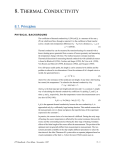
Each vertical heat exchanger consists of three main components, as shown in
figure 1-1. The three components are the pipe, grout material around the pipe, and soil
around the grout. The vertical borehole is a drilled cylindrical hole that can vary in
diameter and depth.
The pipe, which typically ranges from ¾” nominal diameter to 1 ½” nominal
diameter is high density polyethylene (HDPE). The pipe is inserted in a “U” shape, with a
“U-bend” at the bottom of the borehole.
The next component is the material surrounding the pipe, usually “grout”. The
grout plays an important role in heat transfer between the soil and the fluid flowing
within the pipe. It is preferable for the grout to have a high thermal conductivity.
Different grout materials have different thermal conductivity values, typically ranging
from 0.3 to 0.9 Btu/ft-hr-°F.
The goal of this thesis project is to develop an apparatus and procedure for
estimating the thermal properties of the soil surrounding a drilled hole. The uncertainty
of the soil’s thermal properties is often the most significant problem facing GSHP
1
designers and engineers. The thermal properties that designers are concerned with are
the thermal conductivity (k), thermal diffusivity (α), and volumetric heat capacity (ρcp).
The properties are related by the following equation:
α soil =
k soil
ρ soil c psoil
(1-1)
The number of boreholes and depth per borehole is highly dependent on the soil thermal
properties. Depending on geographic location and the drilling cost for that particular
area, the soil thermal properties highly influence the initial cost to install a ground source
heat pump system.
H D P E P ip e
Grout
Soil
Figure 1-1. Typical Vertical Ground Loop Heat Exchanger with a U-bend Pipe
Configuration
2
Designers of the ground loop heat exchangers have a very difficult job when
estimating the soil thermal conductivity (k) and soil volumetric heat capacity (ρcp). Both
soil thermal properties are generally required when the designer is sizing the ground loop
heat exchanger depth and number of boreholes using software programs such as
GLHEPRO for Windows (Spitler, et al. 1996).
The borehole field can be an array of boreholes often configured in a rectangular
grid. In order to design the borehole field, designers and engineers must begin with
values for the soil parameters. Some engineers and designers use soil and rock
classification manuals containing soil property data to design GSHP systems. One
popular manual used is the Soil and Rock Classification for the Design of GroundCoupled Heat Pump Systems Field Manual (EPRI, 1989). Figures 1-2a and 1-2b are
excerpts from the manual of typical thermal conductivities for the rock classifications.
The horizontal band associated with each soil/rock type indicates the range of thermal
conductivity. The typical designer must choose a thermal conductivity value within that
band range depending on the soil composition of the project.
3
Figure 1-2a. Rock Thermal Conductivity Values Taken from
Soil and Rock Classification Field Manual (EPRI, 1989)
Figure 1-2b. Rock Thermal Conductivity Values taken from
Soil and Rock Classification Field Manual (EPRI, 1989)
4
Consider Quartzose sandstone (ss) wet in Figure 1-2b. According to the figure,
the thermal conductivity ranges from 1.8 Btu/ft-hr-°F (~3 W/m-K) to 4.5 Btu/hr-ft-°F
(~7.85 W/m-K). A conservative and prudent designer would choose the thermal
conductivity value of 1.8 Btu/hr-ft-°F (~3 W/m-K) or some value close to the low end of
the band. The lower conductivity value results in more total borehole length. At the
other end of the spectrum, the high value of 4.5 Btu/hr-ft-°F (~7.85 W/m-K) yields the
smallest total borehole length.
As an example, twelve boreholes in a rectangle are sized for a 9,000 ft2 daycare
center. Using the sizing option of GLHEPRO for Windows and a thermal conductivity
value of 4.5 Btu/hr-ft-°F (~7.85 W/m-K), the required depth for each borehole is 152 ft
(~46 m). With the same configuration, changing the thermal conductivity to 1.8 Btu/hrft-°F (~3 W/m-K) requires a ground loop heat exchanger depth per borehole of 217 ft
(~66 m). This is a per borehole depth difference of 65 ft (~43 m), nearly a 43% increase.
The change in depth greatly effects the change in cost. The borehole will incur
additional drilling cost, pipe cost, grout cost, and header cost. Estimating a cost of $10
per foot for the total installation, the additional ground loop heat exchanger depth will
cost $7,800 for the twelve boreholes.
To even further complicate the problem, the designer must deal with soil rock
formations that consist of multiple layers. In order to overcome this uncertainty, the
designer may require that a well log as a single test borehole is drilled. Unfortunately,
well logs are often extremely vague (“…12 feet of sandy silt, 7 feet of silty sand…”) and
difficult to interpret. When the uncertainties in the soil or rock type are coupled with the
5
uncertainties in the soil thermal properties, the designer must, again, be conservative and
prudent when sizing the borefield.
This thesis focuses on methods for experimentally measuring the ground thermal
properties using a test borehole, then using the experimental results to develop methods
to better estimate the ground thermal properties. All of the tested boreholes were part of
commercial installations and research sites in Stillwater, OK, Chickasha, OK, and
Bartlesville, OK, and South Dakota State University, SD. This thesis will describe the
development an experimental apparatus to collect data and the development of a
computational model to evaluate the data collected and estimate the soil thermal
properties.
1.2. Literature Review- Test Methods
There are several methods for estimating soil thermal conductivity that might be
applied to boreholes. These include soil and rock identification, experimental testing of
drill cuttings, in situ probes, and inverse heat conduction models.
1.2.1. Soil and Rock Identification
One technique to determine the soil thermal properties is described by the IGSHPA
Soil and Rock Classification manual. The manual contains procedures to determine the
type of soil and the type of rock encountered at a project location. The procedure begins
by classifying the soil by visual inspection.
6
The next few steps can be followed by the flow chart depicted in figure 3-1 of the Soil
and Rock Classification Field Manual (EPRI 1989). Once the soil type has been
determined, the reference manual offers the values shown in Table 1-1 for the different
soil types:
Thermal Texture
Class
Sand (or Gravel)
Table 1-1 Soil Thermal Properties
Thermal Conductivity
W/m-°K
Btu/hr-ft-°F
0.77
0.44
Thermal Diffusivity
cm2/sec
ft2/day
0.0045
0.42
Silt
1.67
0.96
-
-
Clay
1.11
0.64
0.0054
0.50
Loam
0.91
0.52
0.0049
0.46
Saturated Sand
2.50
1.44
0.0093
0.86
Saturate Silt or Clay
1.67
0.96
0.0066
0.61
Alternatively, if the underlying ground at the site also contains various rock
formations, it is then necessary to classify the rock type(s) into eight different categories
based upon several different elements. The eight categories are termed Petrologic
groups. Figure 1-2a and 2b show the thermal conductivity values for each rock type.
Even though the rock identification procedures are somewhat complicated, the designer
is still left with a wide range of thermal conductivities and to be prudent, must choose a
low value.
1.2.2. Experimental Testing of Drill Cuttings
Another method used to determine the thermal conductivity of the rock was
approached from the viewpoint that the conductivity can be determined from the drill
cuttings. Sass (1971) stated at that time that thermal conductivity is difficult to determine
7
by standard methods due to the lack of cores or outcrop samples from the drill. The
only available samples to use were the drill cuttings that could vary in size from a fine
powder (air-drilled displacement) to millimeter sized particles (coarse-toothed rotary
bits). Sass (1971) began his procedure by collecting the drill cuttings of a well into a
plastic cell using a spatula to pack the particles inside the cell. The plastic cell is then
weighed (dry). Then water is added into the plastic cell and weighed again (wet). The
difference in weight can be used to find the volume fraction of water. Next, the cell is
placed in a divided-bar apparatus and the effective thermal conductivity is determined.
The plastic cell is a long plastic tube approximately 0.63 cm thick, fitted to machined
copper bases as shown in Figure 1-3. The outer diameter is the same as the divided bar
at an outer diameter of 3.81 cm and an inner diameter of 3.49 cm. The plastic cell has a
volume of 6 cm3. A constant temperature drop is maintained across the sample and
copper standard. The thermal conductivity is then estimated by using a rock fragment
and water mixture in a steady-state divided-bar apparatus.
Figure 1-3. Illustrated Thermal Conductivity Cell
8
The model for this approach begins with the assumption that the thermal
resistance of the full cell can be represented by the thermal resistance of the aggregate
and the plastic cell wall in parallel given in equation 1-2.
Ka =
Where,
D2
D2 − d 2
K
−
Kp
d2 c
d2
(1-2)
Kp is the thermal conductivity of the plastic wall
D is the Outer diameter of the Cell Wall (3.81 cm)
d is the Inner Diameter of the Cell Wall (3.49 cm)
Kc is the measured conductivity of the Cell and Contents
Ka is the conductivity of the water-saturated aggregate.
In the second part of this model, the aggregate can be represented by a geometric
mean of conductivities of its constituents. Where the constituent conductivities do not
contrast by more than one order of magnitude, this model appears to have been
successful for applications of this kind. For an aggregate in which the ith constituent
occupies volume fraction φ,
K a = K1φ 1 K 2 φ 2 .... K n φn
(1-3)
If n-1 of the constituents are solid fragments, and the remaining constituent is
water with conductivity Kw and volume fraction φ, then Ka becomes:
K a = K r 1− φ K w φ
Where,
(1-4)
Kr is the geometric mean conductivity of the solid constituents
Combining equation 1-1 and 1-3 gives:
D2 K
D2 − d 2 K p 
Kr = Kw  2 c −

Kw 
d2
 d Kw
1/ ( 1− φ )
Substituting the known numerical values and the known values of the apparatus,
equation 1-5 can be reduced to:
9
(1-5)
K r = 1.46{ 0.815K c − 0104
. }
1/ ( 1− φ )
(1-6)
Equation 1-6 gives an estimate of the conductivity of a nonporous isotropic rock in
terms of the effective conductivity of a cell containing its water-saturated fragments and
of the porosity of the cell’s contents.
The results of using this method to determine the thermal conductivity are
debatable due to the assumption of rock/soil continuity. If several different layers of
rock and/or soil are present, it is difficult to determine with certainty the thermal
conductivity value obtained using the drill cuttings. 1
1.2.3. In Situ Probes
The idea of using measuring probes has been around for some time. According
to Choudary (1976), sampling the ground parameters for thermal conductivity and
diffusivity in situ using a probe could reduce measurement error of the ground thermal
conductivity. This concept was first suggested by a German physicist named
Schleiremachen in 1833. It wasn’t until around the 1950’s that the probes were
developed to the point of being usable for testing drilled wells.
The general construction of an in situ probe consists of an internal heater and at
least one embedded temperature sensor all set in a ceramic insulator or epoxy. All of
1
Experimental Testing of Borehole Cored Samples
Concurrent research under way at Oklahoma State University in estimating the thermal conductivity of
the soil uses the concept of cored samples taken from a borehole drilled for use in a ground loop heat
exchanger. This new innovative method takes cored samples from the drill and utilizes a guarded hot
plate experimental test apparatus. Each core sample tested is the size of small cylinder with
approximately 3 ½” radius and 3” in length. The sample is carefully handled to maintain the moisture
content by sealing the sample with a very thin layer of epoxy.
10
these components are then encased by a metal sheath, usually stainless steel on modern
probes.
Most probes used for this type of application today are about 6 to 12 inches long.
These types of small probes are usually placed in a bucket size sample of the drilled soil
at a laboratory. The probe in the middle of the bucket then heats the soil. The probe
then measures the temperature response to the heat input. Some newer probe models
incorporate the heater and temperature sensor within the same probe. Based upon the
temperature measurement in the middle of the probe and the measured heat input, the
results are used in models such as the Line Source Model for determining the thermal
conductivity of the soil.
1.3. Literature Review- Models
Several different models have been utilized for estimating the performance of
vertical ground loop heat exchangers. They are of interest here for possible inverse
use—estimating the ground thermal properties from the performance rather than the
performance from the ground thermal properties. Specifically, we are interested in
imposing a heat pulse of “short” duration (1-7 days) and determining the ground thermal
properties from the results.
11
1.3.1. Line Source Model
This model is based on approximating the borehole as a line source, assuming
end effects are small. The soil acts as a heat rejection medium that has an assumed
uniform and constant initial temperature (To). The original model was first developed by
Lord Kelvin and it is sometimes called Kelvin Line Source Theory. Ingersoll and Plass
(1948) applied the model to ground loop heat exchangers. Mogensen (1983) further
enhances their findings by applying the model to estimate the ground thermal
conductivity. Ingersoll and Plass begin with this general line source equation:
Q&
∆T (r , t ) =
2πk
∞
∫
−β
e
r
2 πk
β
2
dβ
(1-7)
Where,
∆T(r,t) = Temperature Rise beginning at To (°F)
r = Radius from Line Source (ft)
t = Time after start of Heat Injection (hr)
Q& = Heat Injection Rate per unit borehole length (Btu/hr-ft)
k = Thermal Conductivity (Btu/hr-ft-°F)
α = Thermal Diffusivity (ft2/hr)
Mogensen (1983) suggested approximating the integral portion of equation 1-7
as:
∞ e−β 2
 4αt 
∫
dβ = ln
−C
 R2 
β
r
2πk
Where,
C = Euler’s Number (0.5772…).
12
(1-8)
In this case, r = R is the borehole wall radius given by Mogensen (1983). It is
also required to include the thermal resistance between the fluid within the pipe and the
borehole wall. Mogensen (1983) stated this thermal resistance as ‘mTR’.
The thermal resistance has the units of hr-ft-°F/Btu. The addition of thermal resistance
into the equation yields:
∆T ( R , t ) = Q& mTR +
Q&   4αt 

ln
−
C



4πk   R2 

(1-9)
Collecting terms and rearranging the equation to a more usable form, it becomes easily
evaluated for an effective thermal conductivity of the soil for a given length of time, near
constant heat injection rate, and near constant change in temperature. The resulting
equation for this evaluation is:
∆T ( R , t ) = Q& m TR +
Q&   4α 
 Q&
ln
ln t
 − C +
4πk   R2 
 4πk
(1-10)
Notice the first two terms on the right hand side of the equation are constant as
long as the heat injection rate is near constant. The only variable in the equation is ln(t).
The equation is then reduced to simplest form by taking the constants and ln(t) into a
general linear form,
y = mx + b
Where,
y = ∆T the change in temperature
b = the two constant terms on the RHS of the equation
m=
Q&
4πk
x = ln t
13
(1-11)
After obtaining experimental data of delta T, time, and the heat injection rate, a
simple plot of temperature versus the natural log of time will yield the slope of the line.
This slope is equated to ‘m’ and the thermal conductivity can be determined.
This model is very easy to use once the derivation is reduced to the final equation
(1-11). The Line Source Model does have some disadvantages. This model is applied in
Chapter 5. As shown in Chapter 5, there are significant difficulties associated with
applying the model in practice.
1.3.2. Cylindrical Source Model
The model was first implemented by Carslaw and Jaeger and presented by
Ingersoll (1948, 1954). The description here relies primarily on Kavanaugh (1984,
1991). The model was developed by using a finite cylinder in an infinite medium of
constant properties. The cylinder source model begins with the analytical solution to the
2-D heat conduction equation:
∆Tg = T ff − Tro =
q gc
ks L
G ( z , p)
(1-12)
1 ∞ e −β z − 1
dβ
Where, G ( z , p) = 2 ∫ 2
J 0 ( p β ) Y 1 ( β ) − J 1 ( β ) Y 0 ( pβ ) 2
2
β
π 0 J 1 (β ) + Y1 (β )
2
[
]
Tff is the far-field temperature
Tro is the temperature at the cylinder wall
Tg is the temperature of ground
qgc is the heat flux or heat pulse to the ground
ks is the thermal conductivity of the soil
L is the length of the cylinder
14
(1-13)
The dependent variables within the ‘G’ or cylinder source function are given as:
z=
p=
α soil t
(1-14)
r2
r
ro
(1-15)
The term z in equation 1-14 is known as the Fourier number. Equation 1-12 is
based on a constant heat flux to the ground. For the purposes of experimentation and
the fact that applications do not operate in the constant heat flux mode, equation 1-12
can be modified to adjust for the abnormalities that occur. Kavanaugh (1991) has
developed an equation to estimate equation 1-12, broken down into piece-wise time
intervals. The resulting equation is:
∆Tg =
[
]
[
]
 RF1q gc G( z , p) − G ( z , p)
+ RF2 q gc2 G( z , p) n −1 − G( z , p) n − 2 + 

n
n −1
1

 (1-16)
k soil L ...+ RF q G ( z , p)

n gcn
1

Where,
1
[
]
RF is the run fraction that modifies the heat rate into the ground
(Kavanaugh, 1984)
n is the time interval
In order to adapt the cylinder source model to a borehole with a U-bend pipe
configuration, an equivalent diameter was suggested to correct this error. The diameter
of the two pipe leads can be represented by an approximation of an equivalent diameter
for the given pipe’s diameter (Bose, 1984).
Dequivalent =
2 Do
(1-17)
This diameter equivalence of equation 1-17 yields a single diameter pipe, which
approximates the heat transfer from two pipes in a cylindrical borehole. The two pipes
are represented as a single cylinder with diameter Dequivalent . If the grout properties are
assumed to be the same as the soil properties, the temperature at the edge of the
15
equivalent pipe can be estimated using G(z,1). The resistance between the fluid and the
edge of the equivalent pipe must be estimated. The internal structure is composed of the
resistance of the pipe conductivity and the resistance of convection due to the fluid
movement inside the pipe. The pipe resistance can be represented 2 by:
r 
ro ln o 
 ri 
Rp =
2k p
(1-18)
The conductivity of the pipe (kp) is required as part of the input for equation 1-18.
The convection resistance can represented similarly by:
1
ri
hi
ro
Rc =
(1-19)
The convection coefficient (hi) in equation 1-19 is determined from the following two
equations that deal with heat transfer in internal fluid flow pipes. Equation 1-20 is the
convection coefficient for turbulent flow.
hi = Nu Di
kw
Di
(1-20)
The Nusselt number (Nu) is given by Dittus (1930) as a function of the Reynold’s
number and Prandtl number. The Nusselt equation is given as:
Nu Di = 0.023 Re 4D/i5 Pr n
(1-21)
The Prandtl power coefficient is dependent on the direction of the temperature field. For
heating (Tpipe surface > Tmean fluid temp), n = 0.4. For cooling (Tpipe surface < Tmean fluid temp), n =
0.3.
2
Kavanaugh does not insert a 2 in the denominator, but it appears that it should be there to account for
the fact that there are two pipes in parallel. Cf. Paul (1996).
16
After calculating the convection coefficient in equations 1-20, equation 1-18 and 1-19
can be combined into an equivalent heat transfer coefficient of the total heat transfer
from the fluid to the outside cylinder pipe wall. Kavanaugh (1991) represents the
equivalent pipe resistance as:
heq =
1
R p + Rc
(1-22)
The temperature difference between the outside wall of the cylinder and fluid inside the
pipe can be calculated using equation 1-23.
∆Tp =
q gc
C * N t * heq * Ao
(1-23)
Where, Ao = 2πroL is the outer surface area of contact
C = 0.85 is the short circuit factor
Nt is the number of tubes used
The combination of two pipes configured in a U-bend borehole are close together
if not touching at some places. Since the result is some heat transfer from one pipe to
the other (thermal short-circuiting), Kavanaugh (1984) has incorporated a coefficient to
account for this. The coefficient is C = 0.85 for a single U-bend ground loop design.
There is also a need to account for the actual number of pipes. Occasionally, more than
one U-tube is inserted into a borehole, the coefficient Nt accounts for the additional
actual surface of the multiple pipe leads.
After determining all of the variables, equations 1-12, 1-22 and the far-field
temperature (Tff) can be summed to yield the average water temperature.
Tavg = Tff + ∆Tg + ∆Tp
17
(1-24)
As presented, the cylinder source model does not account for the grout thermal
properties, but they could be taken into account. Kavanaugh (1997) suggests a trialand-error approach to determine ksoil from an experimental data set. This is not wholly
satisfying, as it is time consuming and relies on user judgement as to what is the best
solution.
18
1.4. Objectives
Based on the need for measurement of ground thermal properties, the following
objectives have been developed:
1. Develop a portable, reasonable-cost, in situ test system that can be replicated by
others in the ground source heat pump industry. Also, determine a suitable test
procedure.
2. Develop a numerical model to represent a borehole, incorporating variable power
input, convection resistance, conduction through the pipe, conduction through the
grout, and conduction through the soil. The model will be used to determine the
thermal response of the borehole and ground for various choices of soil and grout
thermal properties. By adjusting the value of the soil and grout thermal properties, a
best “fit” to the experimental data can be found. The adjustment process, when done
systematically, is known as parameter estimation.
3. Determine the best parameter estimation procedure for analyzing the experimentally
obtained results of the soil thermal properties.
19
2. Experimental Apparatus
2.1. Description of Experimental Apparatus
The experimental apparatus is contained within an enclosed single axle trailer.
The trailer contains all necessary components to perform a test. The apparatus has two
barb fittings on the exterior of the trailer to allow attachment of two HDPE tubes which
are protruding from a vertical borehole. The trailer houses stainless steel plumbing,
water heater elements, water supply/purge tank and pump, circulation pumps and valves,
an SCR power controller, and two 7000 watt power generators (not inside the trailer
during testing). All necessary instrumentation and data acquisition equipment are also
contained within the trailer. The instrumentation and data acquisition equipment include
a flow meter, two thermistor probes, a watt transducer, two thermocouples, and a data
logger. The experimental apparatus is described as a set of subsystems: the trailer, the
water supply, the power supply, water heating, pipe insulation, temperature
measurement, flow sensing/control equipment, and data acquisition.
2.2. In Situ Trailer Construction
The in situ trailer must be able to operate independently of water and electric
utilities, since many of the test locations are undeveloped. The trailer must also be
capable of housing every component of the experimental apparatus. The mobile unit
containing the experimental apparatus is a Wells Cargo general-purpose trailer. Figures
2-1 and 2-2 are scaled drawings of the Wells Cargo/In Situ trailer. Both figures depict
20
exterior views of the trailer, and show the original condition of the trailer with one
modification, the Coleman 13,500 Btu/hr Air Conditioner mounted on top of the roof.
Air Conditioner
Figure 2-1. Exterior Views of In Situ trailer
Figure 2-2. Exterior Views of In Situ trailer
The dimensions of the trailer play a very important role in equipment placement.
All other parts of the experimental apparatus must fit into the trailer at the same time.
The inside trailer dimensions are 10 ft x 6 ft x 5 ½ ft, shown in Figures 2-3 and 2-4.
21
5.500 ft.
10.000 ft.
6.000 ft.
Figure 2-3. In Situ Trailer Dimensions
Water Tank
9.528 ft.
10.0 ft.
5.250 ft.
6.000 ft.
Figure 2-4. Top View of Trailer
22
Interior and exterior modifications are required to the trailer for the experimental
equipment. The first modification to the trailer is the interior wall reconstruction. The
trailer was acquired with 1/16” aluminum exterior siding and 1 ¼” steel frame beams to
support the siding and interior walls. The interior walls were 1/8” plywood mounted to
the steel beams. Insulated walls were not included with the purchase of the trailer. With
the interior walls as delivered, there was not any room for installation of the insulation
and electrical wiring designed for the space nor was the wall capable of supporting the
plumbing mounted directly to the inside wall. To overcome these problems, several
changes and additions are made to the trailer.
First the steel frame beams are extended in order to create more space in between
the interior and exterior walls. Wood studs are mounted to the steel beams on the inside
surface of the beam. Since the frame beams are a U-channel shape, the studs fit in the
middle of the U-channel. As the studs are mounted to the beams, the studs wedge into
the channel creating a sturdy wall. Figure 2-5 is an overhead view of a cross section of
the new left side wall construction. The studs are 3 ½” wide and 1 ½” thick, a normal
2x4 construction grade stud. This gives a new total distance between the exterior
aluminum siding and the inside surface of the interior wall of approximately 4 ½”. The
gap is filled with two layers of R-11 insulation (compressed), to minimize heat loss
through the wall to the outside air (the total R-value of the wall is about 24). In
addition, conduit is installed through the wood studs for the required electrical wiring.
23
16.0 in.
Steel
C h an n e l
Bracket
2 x4 Stud
3/4 in. Plywood
1/16 in.
Alumi n u m S i di n g
Fiber g l a s s Insulati o n
5.9 in.
Figure 2-5. Overhead View of the Left Wall Cross Section
The inner layer of the trailer in Figure 2-5 is ¾” plywood which provides
structural support for mounting brackets and screws. It is essential since the stainless
steel plumbing weighs approximately 80 lbs.
The rest of the interior walls of the trailer are constructed in the same manner as
in Figure 2-5. The only difference for the other internal walls is the ¾” plywood is
replaced with ½” plywood to allow for attachment of other items. The rear and side
access doors were not modified; they are already insulated and did not require changes.
24
Another modification for the trailer is the installation of the Coleman Air
Conditioner. Some temperature measurement devices, e.g. thermocouples with cold
junction compensation, are sensitive to temperature fluctuations. When the local
temperature fluctuates, a temperature differential is created between the thermocouple
junction and the cold junction compensation temperature, causing an error. The
experimental test requires at least one person to operate the experiment. The air
conditioner is capable of producing 13,500 Btu/hr or 1.125 tons of cooling. For the size
of the trailer, the air conditioner has more than enough capacity to meet the space
requirements. To minimize these errors, a constant conditioned space temperature is
desirable. Therefore, a second design need is met with the air conditioner.
2.3. Water Supply System
In order to keep the experimental apparatus mobile, a water supply tank and
purging system must accompany the system. If water is not readily available at a test
site, the water supply tank can be used to fill the plumbing system inside the trailer and, if
required, the borehole pipe loop. The water supply system is composed of six different
components:
1.
2.
3.
4.
5.
6.
Water Storage
Water Purging
Water Flow Rate
Water Filtering
Water Circulating
Water Valve Control
25
2.3.1. Water Storage Tank
The first component of the water supply system is the water storage tank. The
tank is molded out of ¼” thick, chemical resistant polyethylene. The water storage tank
is rectangular in shape and has the dimensions of 18”h x 17.5”w x 36.5”l. It is capable
of storing a maximum of 45 gallons of water. The tank has 3 inlet/outlet ports. Figure
2-6 is a drawing of the tank with the location of the three ports relative to the position of
the tank inside the trailer depicted. The tank is located on the front wall of the trailer.
The top view in Figure 2-6 is illustrated looking towards the front wall of the trailer
inside of the trailer. The bottom view is the left side view of the tank and the inlet/outlet
ports. The water supply and return ports connect to a flow center* mounted on the left
side trailer wall.
Water Fill Location
Water Return Line
Water Supply Line
Water Drain Line
Front View
Water Return Line
Water Supply Line
Side View
Water Drain Line
Figure 2-6. Water Supply Flow Ports
*
A “flow center” is a metal cabinet containing 2 pumps, each connected to a 3-way valve. They are
commonly used in residential GSHP installations.
26
One port is the water supply line, located at the bottom of the water storage tank.
This allows the purge pump to draw water that does not contain air bubbles. The second
port is the water return line, located near the top of the water storage tank. This allows
any air in the water purged from the borehole or the plumbing system inside the trailer to
bubble out the top portion of the tank. Returning water to the top of the tank minimizes
the air bubbles in the water being drawn out of the bottom of the tank. The third port is
the drain line, located at the bottom of the tank near the water supply line. The water
drain line in the water tank can drain the entire system if it is needed. Each port has a
PVC ball valve on the exterior left side of the tank. The ball valves allow an operator to
shut off the tank ports after the completion of the purge test.
2.3.2. Water Purging
The second component of the water supply system is the purge pump system.
The two purge pumps are connected to the water supply tank via the water supply line.
Figure 2-7 is a frontal view of the water supply system. The pumps are mounted in-line
and vertically with the 1” PVC plumbing. The pumps serve to circulate the working
fluid during the purging operation of a test. The Grundfos pumps are located on the left
side of the ball valve on the water supply line. The Grundfos pumps are UP26-99F
series pumps rated at 230V and 1.07A. Under normal working conditions they supply 8
gpm to the plumbing inside the trailer at 10 psig and produce 7 gpm to a 250ft borehole
at an unmeasured pressure. The flanges for the pumps connect with 1” nipple pipe
thread (NPT)-1”PVC 40 nominal schedule fittings.
27
2.3.3. Water Flow Rate
The third component of the water supply system is the visual flow meter. It is a
CalQflo flow meter and serves to evaluate the flow rate when the borehole line or the
internal plumbing is purging (A separate, high quality flow meter, described below, is
used to measure flow rate during the experiment.). The location of the flow meter is
down stream from the purge pump. The reading from the visual meter is an indicator of
correct flushing speed. There is not any data collection during the purging operation.
The flow in the internal plumbing during purging is moving in the opposite direction of
the instrument flow meter; therefore that reading can not be reliable because the flow
meter is unidirectional. The overall reason for using the visual flow meter is to
determine if flow rate is fast enough to purge the system. There is a minimum
requirement of 2 feet per second to purge air out of a system line (IGSHPA, 1991). If
the minimum requirement is not met, then air remaining in the system will interfere with
the flow rate measurement.
2.3.4. Water Filtering
The fourth component of the water supply system is the water filter. The water
filter is in between the visual flow meter and the purge pumps in the water supply line.
The water filter is a standard in-line filter cartridge normally used with household water
systems to remove excess rust and sediment. The water filter serves as a particle
removal filter, removing sediment, rust, or other foreign particles such as HDPE
28
shavings flushed from the U-tube or the rest of the system. The filter also aids in
maintaining a minimum constant head on the purge pump.
Breaker Box #2
Breaker Box #1
In-Line Visual Flow Meter
Goes Here
Cartridge Filter
Purge Pumps
Water Tank
Drain Line
Shut-off Ball Valves
Figure 2-7 View of Front Wall Depicting the Water Supply/Purging Equipment
2.3.5. Water Circulating Pumps
The fifth component of the water supply system is the circulating pump system.
The circulating pump system is composed of two pumps placed just after the water filter
as seen in Figure 2-8. These pump are also Grundfos UP26-99F series pumps. They are
29
230Volt/1.07Amp pumps. The design of the plumbing makes use of the pumps physical
characteristic ability to mount in-line. The advantages of using the in-line pumps as
opposed to other pumps are simple mounting, easy installation, and minimal maintenance
time. The circulating pumps aid in purging the U-bend and pressurizing the system line.
When the purge pump and the two circulating pumps purge the U-bend, they produce 910 gpm flow for a 250 ft deep borehole using ¾” nominal pipe.
Water Supply Line
Circulating Pumps
Flow Center
Water Return Line
3-Way Valves
Figure 2-8. Left Side Wall View of Water Circulation Pumps and Flow Control
Valves
2.3.6. Water Valve Control
The sixth component of the water supply system is the flow direction control
valve system shown in Figure 2-8. The valves can direct water in a number of different
flow patterns. These valves are very small and easily turned. The different flow patterns
used during purging and experimental testing can be seen in Figure 2-9. During the
purging operation of a test, flow pattern A is set first to purge the borehole line only, for
30
approximately 15-20 minutes. The purge time is set to IGSHPA standard I.E.7. of the
Design and Installation Standards (IGSHPA, 1991). Flow pattern A creates an open
loop with the water supply tank and flushes the line at approximately 8 gpm. After
purging the borehole line, flow pattern B is set to purge the stainless steel plumbing
inside the trailer for about 15-20 minutes. This flow pattern also creates an open loop
with the water supply tank and flushes the plumbing at approximately 5 gpm. Next, flow
pattern C is set to purge both the borehole loop and the stainless steel plumbing for an
additional 10 minutes. Finally, flow pattern D is set to close the system off from the
water supply tank. This creates a closed loop system, circulating the fluid continuously.
Flow Direction
Flow Direction
Flow Direction
A
B
C
Flow Direction
D
Figure 2-9. Flow Pattern of Flow Control Valves
2.4. Power Supply
The power supply for the experimental test consists of two Devillbiss gasoline
generators. Each generator is capable of supplying 7000 Watts. They are supplied with
wheel kits, allowing the generators to move in and out of the trailer on ramps. Included
in this subsystem is all wiring and wiring accessories the electrical system.
31
The generators are configured and placed outside of the trailer toward the front
left side of the trailer, when possible. Each generator is set to deliver 240 volts. Two
power lines, one from each generator, are routed from the generators to outside
receptacles located in the front trailer wall. The main breaker boxes are located on the
same front wall inside of the trailer, shown in Figure 2-7. Separate generator powers
each breaker box. The breaker box #1 handles the power requirements for the water
heater elements and the two circulating pumps. The breaker box #2 supplies power to
the rest of the trailer. The second breaker box contains the purge pump breaker, the A/C
breaker, and two plug in receptacle breakers. The computer/data logger,
instrumentation, and any other standard 115V power item in the trailer use the outlet
receptacles.
2.5. Water Heating Method
The circulating water inside the closed loop system is heated with (up to) three
in-line water heaters. The water heaters are ordinary water heating elements used in
residential water heaters. Each water heater element has a screw-in mount for 1” NPT
connections and is screwed into a tee joint, as shown in Figure 2-10.
32
1.0 kW Element
1.5 kW Element
2.0 kW Element
Figure 2-10. Heat Element Locations in Stainless Steel Plumbing Layout
The heater element #1 is rated at 1.0 kW, heater element #2 is rated at 1.5 kW,
and heater element #3 is rated at 2.0 kW @ 240 volts. The design of the heater system
allows the in situ system to vary the range of heat input between 0.0 kW and 4.5 kW.
The 2.0 kW heater is connected to a Silicon Controlled Rectifier power controller, which
can vary the power between 0 kW and 2.0 kW. By varying the power to this element
and switching the other two elements on or off, the entire range of 0.0 - 4.5 kW can be
achieved. The power controller for the 2.0 kW heating element is a SCR power
controller with a manual potentiometer for varying the full output as a percentage. The
location of the SCR power controller is shown in Figure 2-11. The manual
potentiometer is mounted next to the LED digital display for the power input. It can be
seen in Figure 2-18.
33
As the water flows clockwise within the plumbing in Figure 2-10, it flows across
each water heater element. The direct contact with the flowing fluid in a counter flow
fashion optimizes the amount of heat transferred from the heater elements to the fluid.
This further reduces transient heat transfer effects, as compared to using the same heater
elements in a tank* (an early design concept). Also, the power measurement is used to
determine the heat flux in the borehole, and a tank adds an undesirable time lag between
the power measurement and the heat transfer to the borehole.
SCR Power Controller
Figure 2-11. SCR Power Controller Location
Total energy input to the circulating fluid is measured by a watt transducer. The
total energy is the energy from the heater elements and the energy from the circulating
pumps. Early tests indicated that the circulating pumps are a significant source of heat
input, on the order of approximately 300 to 400 watts.
*
Another trailer, built by a commercial firm, utilized a water tank. The tank was subject to sudden
changes in exiting water temperature when (apparently) the water in the tank was experiencing
buoyancy-induced instability.
34
2.6. Pipe Insulation
The stainless steel plumbing is insulated to aid in reducing heat loss. All piping
contained within the trailer is insulated using a fiber glass material called Micro-Lok
insulation shown in Figure 2-12.
Zeston PVC 90° Elbow
Micro-Lok Insulation
Figure 2-12. Inside Pipe Insulation
In Figure 2-10, the stainless steel pipe was not yet covered. Figure 2-12 depicts
all plumbing components insulated with the exception of the flow center. The MicroLok pipe insulation is 1 ½” inches thick with an R-value of approximately 5.5 (hr-ft2-°F/
Btu). Micro-Lok is chosen due to its “hinged” siding to easily wrap around each pipe
length and formidable compressed fiberglass structure for custom fitting at awkward pipe
joint locations. Zeston PVC fittings are also used to cover and insulate special joint
locations such as each tee joint with the water heater elements.
35
It is also necessary to insulate the exterior exposed pipe leads from the U-bend.
Figures 2-13, 2-14, and 2-15 depict the insulation of the exterior pipe. Early tests
revealed considerable heat loss through the exterior pipes if they were not well insulated.
The heat loss is due to the distance from the ground surface to the trailer hook-up
connectors that can vary from just a few feet to as much as 20 or 30 feet. Some
insulation was in use, but a larger R-value improved the overall heat balance difference.
½” Foam Insulation
¾” Pipe
5” Round Duct
9” Round Duct
Figure 2-13. Insulation of the Exterior Pipe Leads from a U-bend
First, 1/2” foam insulation is placed around the exterior pipe leads as shown in
Figure 2-13. Next, the 5” round duct insulation is pulled around the foam insulation.
Finally, the 9” round duct insulation is pulled on top of the 5” round duct insulation.
The R-value of each round duct section is 6 (hr-ft-°F/Btu). Combining the insulation
36
thermal resistances, the foam insulation, and estimating the air gap, the total R-value of
thermal resistance is approximately 18.75 (hr-ft-°F/Btu)*.
Figure 2-14. Exterior Insulation Connecting to the Trailer
After the exterior pipe leads are insulated, they are connected to the exterior barb
connections of the trailer, shown in the left-hand picture of Figure 2-14. Once the
connections to the barbs are complete, the remaining round duct insulation is pulled over
the exterior barb fittings and taped to the side wall of the trailer as seen in the right hand
picture of Figure 2-14. The round duct insulation is then adjusted to ensure it covers all
of the exterior pipe leads exposed out of the ground displayed in Figure 2-15.
*
All of the tests performed before January 1, 1997 were not insulated as described in this section. Only
the ½ inch foam insulation and crude wrapping of fiberglass batt insulation was used during the
previous tests. Effects of changes in the weather are clearly visible in the test data. See, for example, in
Appendix C, the test data of Site A #5 on 11/25/96, which shows a cold front coming through. The
effect of the cold front can be seen in Figure 5-5.
37
Figure 2-15. Round Duct Insulation Covering Pipe
2.7. Temperature Measurement
The water temperature is measured at the inlet and outlet to the trailer, as shown
in Figure 2-16. The sensors for the two temperature measurements are 4 ½” stainless
steel Omega ON-410-PP series thermistor probes with 1/8” NPT fitting. The probes
have an accuracy of ±0.18°F for 2252Ω@25°C. The probes are immersed in the
circulating fluid.
Thermistor Probe
Location
Flow Needle Valve
Figure 2-16. Temperature Probe Location on the Inner Trailer Wall
A digital display meter receives the signal from a probe. The two digital display meters
are Omega DP25-TH-A series digital display meters with analog output boards. The
38
accuracy of the meters is ±0.3°F. The meters can sense a temperature from -112 to 302
°F. The analog output is pre-set by the manufacturer to be 0-10Vdc for the user
specified temperature range. For this experiment 0-10Vdc represents a temperature
range of 50-150°F. The data logger can retrieve the analog signal.
In addition, several temperature measurements are taken using type-T
thermocouples manufactured by Omega. The outside air temperature and inside air
temperature are both measured. Each thermocouple as well as the other temperature
sensing instrumentation is calibrated. The calibration procedure is detailed in chapter 3.
2.8. Flow Sensing/Control Equipment
Precise monitoring of the circulation flow rate is essential to compute an accurate
heat balance. The flow sensing equipment consists of three basic elements. These
elements are the flow sensor, flow display meter, and the flow control valve.
2.8.1. Flow Sensor
The flow sensor has two ¾” NPT ports. With the ¾” ports, the flow meter
mounts directly into the plumbing without any special modifications to the pipe system.
The location of the flow sensor with respect to the rest of the system is shown in Figure
2-17. Since the flow meter adapts so well to the existing plumbing layout, the
connection ports of the flow meter serve as union disconnection joints for our plumbing
system should any work or maintenance to the plumbing be required. This allows us to
maintain the plumbing in sections. The flow sensor is an Omega FTB4607 model. It has
39
a range of 0.22 gpm to 20 gpm. The flow sensor features a high frequency pulse output
from a spinning paddle that rotates about a vertical axis. The claimed accuracy is ±1.5%
of the flow rate at 20 gpm and ±2.0% of the flow rate at 0.8 gpm. The flow sensor has
an operating range of 32°F to 190°F. The flow meter is designed for a uni-directional
flow system. An arrow on the flow meter specifies the flow direction. It requires at
least 15 pipe diameters distance upstream and 5 pipe diameters downstream to create a
uniform flow.
2.8.2. Flow Indicator
The flow indicator display is compatible with the flow sensor. It is an Omega
DPF401-A with TTL Level Inputs. It can readily accept the output pulses from the flow
sensor for frequency ranges of 0.2Hz to 20kHz. It does require user specified flow
units, and frequency conversion rate (i.e. the flow sensor is set for 75 pulses/gal of flow
measured, so the meter must be set too using the operating manual). It has an analog
output accessory that sends a voltage reading to the data logger for data collection. The
analog signal is set using the correct conversion units for flow. The procedure is similar
to that of the thermistor probes and should be followed in the user manual of the flow
indicator display. The indicator has preset calibration numbers determined by the
manufacturer. Checks are made routinely to assure the numbers are correct.
40
Flow Meter Location
Watt Transducer
Current Sensors
Figure 2-17. Close-up View of Watt Transducer
2.8.3. Flow Control Equipment
A thermoplastic needle valve controls the flow rate. The location of the needle
valve can be seen in Figure 2-16. The valve has a very sensitive micro-turn adjustment
knob. The knob allows a test to run at a very constant flow rate. This piece of
equipment was chosen to reduce fluid oscillations that sometimes occur with other more
robust and conventional flow valves such as a gate or globe valve.
2.9. Watt Transducer
A watt transducer is put in place to measure power input to the water heater
elements and the circulating pumps. The watt transducer is built and calibrated by Ohio
Semitronics, Inc. The model depicted in Figure 2-17 is PC5-061DY24. One leg of the
line is connected to the watt transducer terminal strip so the transducer can measure the
41
voltage. Two current sensing doughnuts determine the actual current flowing to the
water heater elements and circulating pumps. One leg of each wire set is sent through
one doughnut and the other leg of each wire set is sent through the other doughnut. The
watt transducer has a sensing range of 0 to 20 kW with an accuracy of ±0.5% of full
scale reading. In order to receive better accuracy for our range of 0-2.0 kW, the
electrical wires are wrapped around each doughnut 4 times to reduce the full scale
reading to 5 kW. The watt transducer has an analog output signal of 0-10 volts of fullscale reading. The signal is sent to the Fluke Data Logger and a green LED digital
display. The display can be seen in Figure 2-18. The display configured to have a
readout of power with the units of Watts. If the 2.0 kW water heater is in use, the
display assists in precise power adjustment using the manual potentiometer that is
located next to the display.
2.10. Data Acquisition and Logging
The watt transducer and digital displays’ analog outputs are measured by a Fluke
Hydra Data Logger. Each of the digital displays’ voltage signal is a DC voltage signal
configured on an output scale of 0-10volts for each measurement. The signals sent to
the data logger from the digital displays are:
1. Temperature of water leaving the trailer (Vdc)
2. Temperature of water returning to the trailer (Vdc)
3. Flow Rate (Vdc)
42
In addition, several other measurements are made directly:
1. Watt Transducer (Vdc)
2. Temperature Inside the Trailer (thermocouple)
3. Temperature Outside the Trailer (thermocouple)
As each signal is retrieved, it is stored in two places. The first place the data is
stored is inside the data logger’s own memory. The data is then down loaded at a later
time without losing any measurements. If a computer, via remote or RS-232 connection
controls the data logger, then the data is also stored in a data file setup by the
manufacture’s software program. Figure 2-18 is a picture of the data acquisition system.
The software program allows configuration of the data logger for an
experimental test. The software allows real time plots every time the data input channels
are scanned. Once the data is retrieved by any of the afore mentioned methods, it is
stored in an ASCII data file and can be read by other programs
43
Manual
Potentiometer
Tin (°F)
Flow (gpm)
Tout (°F)
Twall (°F)
Power (Watts)
Fluke Hydra Data Logger
Computer Notebook
Figure 2-18. Typical Data Acquisition System
44
3. Calibration of Experimental Devices
With any experimental apparatus, some uncertainty exists for each measurement.
These errors are then compounded when the measurements are used to compute other
parameters. Therefore, it is desirable to minimize uncertainties by careful calibration of
the sensors and data acquisition equipment. The experiment collects data of three types,
temperature (°F), flow rate (gallons per minute), and input power (watts). Each device
is calibrated independently, and then an overall check is made with a heat balance.
3.1. Temperature Devices
There are three thermistor probes, two thermocouple probes, and one exposed
thermocouple used to measure temperature. Each device serves a separate and specific
purpose. Two of the thermistor probes are used to determine the fluid temperatures
leaving and returning into the trailer. The thermocouple probes measure the ground and
outside air temperatures. The thermocouple measures the inside room temperature.
Some of the devices require extreme accuracy while some can be used with an
acceptable uncertainty of ± 1.0 °F.
3.1.1. Thermocouple Probe and Exposed Junction
Thermocouple
The exposed junction thermocouple is a type-T thermocouple, which measures
the inside air temperature for the duration of each experimental test. The uncertainty is
45
about ±0.56°F (0.3°C) of the reading as stated by the manufacture. The thermocouple
was not calibrated because the error associated with the reading was acceptable.
The thermocouple probe is used to measure the outside air temperature for each
test. This thermocouple probe uses type-T wire and is 6” in length. The connection of
the two wires is an ungrounded junction. A stainless steel casing that creates the probe
portion of the sensing device surrounds the ungrounded junction. Since the temperature
probe is a type-T thermocouple, it has the same temperature sensing range of -454°F to
752°F (-270-400°C). The error is about ±0.56°F (0.3°C) of the reading. Since it was
used to measure the outside air temperature, the thermocouple probe was also
determined to have a reasonable error that did not need to be taken into account for the
overall heat balance equation used as heat loss or heat gain through the wall to the pipe
inside of the trailer. The probe was calibrated in the same manner as discussed in the next
section with the thermistor probes.
3.1.2. Thermistor Probes
The experimental apparatus uses three thermistor probes. The probes measure
the temperature of the water as it leaves the trailer (Tout) and as it enters the trailer (Tin).
The probes are 4 ½” in length with a 1/8” NPT screw thread. The first and second
probes are mounted to a drilled and tapped hex head bolt. The hex head bolt is mounted
to one of three ports of a pipe Tee joint. The third thermistor probe is retained as a
backup for the first two probes, but currently measures the temperature between the wall
46
the pipe is mounted against and the insulation around the stainless steel pipe (Twall). The
thermistors are accurate to ±0.2°F (±0.1°C).
Each thermistor probe is wired to an LED temperature display that in turn has an
analog output signal to be received by the Fluke Data Logger. The error associated with
the LED display is ±0.3°F (0.2°C).
3.2. Temperature Calibration Procedure
Calibrating the temperature devices began by selecting a known source of
constant or near constant temperature. An environmental chamber was selected to
create the constant temperature surrounding. This chamber uses both heating and
cooling to maintain a set temperature. The user can set the temperature of the chamber.
For the calibration, 10°F increments starting at 50°F are the set point temperatures until
the final temperature of 120°F is achieved.
Another thermistor probe calibrated within two decimal places is used as one of
the sources for the known temperature inside the environmental chamber. Two precision
thermometers are also used inside the chamber to read the temperature inside the
environmental chamber. One thermometer is accurate to ±0.1°F and a temperature
reading range of 30°F to 80°F. The second thermometer is accurate to ±0.1°F and a
temperature range of 75°F to 125°F.
Each temperature “system” is intact, as each probe is set inside the chamber,
along with the calibrated probe. A temperature “system” consists of the following:
thermistor probe, thermistor wire from probe to the LED display, LED display, analog
47
output wire from the LED display to the Fluke Data Logger, and the Fluke Data Logger.
This calibration approach will lump each individual component error associated with
each temperature measurement into one total error. Then the calibration coefficients can
be determined for a linear correction. The linear correlation is the same procedure the
manufacturer of the temperature sensing instrumentation uses.
In order to distinguish each temperature measurement separately they are
assigned a color code. The color code key is as follows:
White = (Tin) The temperature measurement of the water coming into the
trailer.
Red
= (Twall) Backup Device; The temperature measurement at the wall.
Green = (Tout) The temperature measurement of the water as it leaves the
trailer.
The 6” thermocouple probe was also calibrated at this time. It maintained a wire length
of approximately 12ft.
After the temperature of the environmental chamber was in equilibrium at 50°F,
readings of the calibrated thermistor probe display were taken over a period of 10
seconds. Then an average value was calculated because the second digit past the
decimal place fluctuated ±0.03 of the average value. Next, a reading was taken on the
precision thermometer that has the applicable temperature range and recorded. Finally,
the channels of each temperature device were scanned and recorded in the internal
memory by the Fluke Data Logger over 10 seconds. The values of each temperature
measurement read by the Data Logger were average in the same manner as the calibrated
48
thermistor probe.
This step was repeated for each 10°F increment until 120°F was
reached.
In order for the LED readout screen to display a temperature, a linear association
between the raw voltage measured and the actual temperature must be manually scaled
to read temperature values. For temperature measurement a conversion must be
determined for the display to calculate for a given input voltage. Equation 3-1 is the
relationship between the temperature and raw voltage. Equation 3-1 takes on the y = mx
+ b linear equation.
T (° F ) =
(150° F − 50° F )
( Raw _ Volts) + 50° F
10 − 0Volts
(3-1)
Table 3-1 shows each reading taken by the Fluke with average values in bold
print. Once the individual values are tabulated, each LED display reading is reduced to
the raw voltage reading. Once the raw voltage is obtained, a statistical regression is
conducted on the values. The regression is linear with residuals set at 2% or
approximately 0.01°F using the Excel 95 data analysis function. The linear regression
follows the same form used in equation 3-1 except new coefficients for the raw voltage
and values for the constant are calculated. Table 3-2 shows every temperature reading
taken in the environmental chamber. All of the temperatures are within ±0.1°F.
Therefore, the thermistor temperature measurement uncertainties are estimated as
±0.1°F.
49
Reading 1
Reading 2
Reading 3
Reading 4
Reading 5
Average
Reading 1
Reading 2
Reading 3
Reading 4
Reading 5
Reading 6
Average
Reading 1
Reading 2
Reading 3
Reading 4
Reading 5
Average
Reading 1
Reading 2
Reading 3
Reading 4
Reading 5
Average
Reading 1
Reading 2
Reading 3
Reading 4
Reading 5
Reading 6
Average
Reading 1
Reading 2
Reading 3
Reading 4
Reading 5
Reading 6
Average
Reading 1
Reading 2
Reading 3
Reading 4
Average
Reading 1
Reading 2
Reading 3
Reading 4
Reading 5
Average
White
49.9
50.0
50.1
50.1
50.1
50.0
60.0
60.0
60.1
60.2
60.3
60.3
60.1
69.8
69.9
70.0
70.0
70.0
69.9
80.4
80.4
80.4
80.4
80.4
80.4
91.3
91.3
91.3
91.3
91.3
91.2
91.3
97.7
97.7
97.8
97.7
97.7
97.7
97.7
109.6
109.6
109.6
109.6
109.6
118.8
118.8
118.8
118.8
118.6
118.8
Red
50.6
50.5
50.5
50.6
50.6
50.6
59.0
58.9
59.0
58.9
58.9
59.0
59.0
70.6
70.6
70.6
70.6
70.6
70.6
79.5
79.5
79.5
79.5
79.5
79.5
89.7
89.7
89.7
89.7
89.7
89.7
89.7
97.7
97.7
97.7
97.7
97.7
97.7
97.7
109.6
109.6
109.6
109.6
109.6
118.8
118.8
118.8
118.8
118.8
118.8
Green
50.5
50.5
50.5
50.5
50.5
50.5
59.0
59.0
59.0
59.0
59.0
59.0
59.0
70.6
70.6
70.7
70.7
70.7
70.6
79.6
79.6
79.6
79.6
79.6
79.6
89.7
89.8
89.8
89.8
89.8
89.7
89.8
97.7
97.7
97.7
97.7
97.7
97.7
97.7
109.6
109.6
109.6
109.6
109.6
118.8
118.8
118.8
118.8
118.8
118.8
TC-Probe
50.7
50.7
50.7
50.7
50.7
50.7
58.9
58.9
59.0
59.0
59.0
59.0
59.0
70.5
70.5
70.6
70.5
70.6
70.6
79.6
79.6
79.6
79.6
79.6
79.6
89.7
89.7
89.7
89.7
89.7
89.7
89.7
97.6
97.6
97.6
97.6
97.6
97.6
97.6
109.5
109.4
109.5
109.5
109.5
118.6
118.6
118.6
118.6
118.6
118.6
Table 3-1. Recorded Temperature Measurements for Calibration Test
50
Table 3-2. Non-Calibrated Temperature Measurements
Calibrated Thermistor
50.6
59.0
70.5
79.4
89.6
97.6
109.5
118.5
Thermometer
50.6
59.0
70.5
79.4
89.6
97.6
109.5
118.5
White
50.0
60.1
69.9
80.4
91.3
97.7
109.6
118.8
Red
50.6
59.0
70.6
79.5
89.7
97.7
109.6
118.8
Green
50.5
59.0
70.6
79.6
89.8
97.7
109.6
118.8
TC-Probe
50.7
59.0
70.6
79.6
89.7
97.6
109.5
118.6
After each regression of the raw voltage, the new calculated coefficient (m) and
the constant (b) can be applied back into equation 3.1 and a new set of temperatures are
determined. The new temperatures are tabulated in Table 3-3.
Table 3-3. Calibrated Temperature Measurements
Calibrated Thermistor
50.6
59.0
70.5
79.4
89.6
97.6
109.5
118.5
Thermometer
50.6
59.0
70.5
79.4
89.6
97.6
109.5
118.5
White
50.6
59.0
70.5
79.5
89.6
97.7
109.4
118.5
Red
50.6
59.0
70.5
79.4
89.6
97.6
109.4
118.6
Green
50.5
59.0
70.6
79.5
89.6
97.5
109.4
118.5
TC-Probe
50.6
58.9
70.5
79.5
89.6
97.6
109.4
118.5
Table 3-4 gives the coefficients and constants for each temperature device. Since
the Fluke Hydra data logger directly monitors the thermocouple probe, it should take on
a near one to one linear relation as seen in Table 3-4.
Table 3-4. New Coefficients for Equation 3.1
Temperature Device
Coefficient (m)
Constant (b)
White
10.00188
50.0775
Red
9.956861
50.06037
Green
9.95378
50.05189
Thermocouple Probe(6”)
1.000241379
-0.07051528
51
3.3. Flow Meter Calibration
The flow meter is calibrated by utilizing a stopwatch and bucket. Three people
work together to collect all of the necessary measurements and readings to calibrate the
flow meter. One person controls the stopwatch and records the actual start and stop
time. Another person runs the Fluke that in turn scans the channel to which flow meter
signal is connected. The last person fills the bucket to a predetermined line and weighs
the bucket of water on a scale. The bucket is marked so that it contains approximately
5 gallons of water. This procedure is performed for several different flow rates
controlled by the needle valve of the pipe system. The calibration occurs at the two
exterior flow ports of the trailer.
Each flow rate requires the following information: Weighing of the bucket
(grams), zeroing out the weight of the bucket by itself, marking time to fill bucket to
approximately 5 gallons, recording actual time began and finished filling the bucket,
scanning the channel for the duration of the time to fill bucket. Once all information is
collected, it is necessary to make use of the conversion of grams to lbm. Once the
conversions are made, the actual flow rate can be determined by the following equation:
•
Q( gal / min) =
MassWater _ in _ Bucket ( lbm)
Time Stop _Watch (min)
*
1
* 7.483( gal / ft 3 )
ρWater ( ft 3 / lbm)
(3-2)
This actual flow rate is compared to the flow rate measured by the flow meter. The flow
meter signal is sent to an LED display box that contains an analog signal output. The
analog signal is read by the Fluke. In order to reduce the uncertainty in the resistance
52
change in the wires and readings of the LED display and data logger, a linear regression
statistical calibration is applied to the raw voltage of the signal of the flow meter using an
Excel spreadsheet using the regression statistical function. This regression was set to fit
the data within a 2% residual. The residual is the statistical function’s ability to find the
coefficients within a percentage of accuracy. The preliminary results indicated the flow
meter was not correctly set.
The new calibrated equation for the flow meter is:
Flow_ Rate(gpm) = 204851529
.
* Raw_VoltageFlow_ Meter − 003807149
.
(3-3)
The results from the calibration test are given in table 3-5. The original flow
meter signal was misreading the flow rate by a factor of approximately two.
Table 3-5. Results from Flow Meter Calibration Procedure
Actual Flow
Measured Flow (gpm)
Calibrated Flow
Error (%)
(gpm)
(gpm)
0.875995
0.432813
0.848553
3.2
1.943090
0.978517
1.966436
1.2
2.839573
1.422996
2.876957
1.3
3.943883
1.927575
3.910595
0.9
3.4. Watt Transducer
The watt transducer measures the amount of power (electricity) transferred to
the water via resistive water heater elements and the circulating pumps. The watt
transducer is calibrated by the manufacturer and has a seal of warranty on the casing
ensuring calibration. The transducer is accurate to ±1% of the reading and ±0.5% of the
full scale reading. The transducer is rated for 20kW, but by looping the wire through the
current sensors four times, the rating is changed to 5kW. The decrease in range
53
increases the accuracy of the readings four fold. The watt transducer has an analog
output signal preset by the manufacturer as 0-10V for the range measured. For our case
it would be 0-10V for 0-5kW. This analog signal is sent to an LED display that in turn
has another analog signal also setup as 0-10V. Those readings are sent to the data
logger.
3.5. Heat Balance
In order to verify the experimental measurements are reasonably, a justifiable
means of validation is required. The approach is to use a heat balance. The simplest
expression of the heat balance equation is:
qin =
62.4(lbm / ft 3 ) * 60(min/ hr )
& p (Tout − Tin )
*Vc
3.414( Btu / hr − Watt ) * 7.483( gal / ft 3 )
(3-4)
Where, qin (watts) is the measured heat input to the water heater elements and
pumps
V& (gpm) is flow rate
cp (Btu/lbm-°F) is the specific heat of water, equal to 1.0(Btu/lbm-°R)
Tin and Tout (°F) are measured from the thermistor probes
After applying all of the calibration equations to the measurement devices, the
heat transfer rate predicted by the right hand side of equation 3-4 can be compared to the
measured power input (left hand side of equation 3.4). The numbers summarized in
Table 3-6 are the average values over the length of each test and they are used to
compare the instrumentation uncertainties and total heat input error.
54
Table 3-6. Heat Balance Check
Location
and Date
Watt Transducer Reading
(Watts)
.
Average
Vcp(∆T) (Watts)
Difference
(Watts)
% of Total
Average Power
Site A #1
1-6-97
Site A #2
1-9-97
Site A #3
2-27-97
Site A #4
3-5-97
Site A #5
4-21-97
Site A V1
4-29-97
Site A #2
5-28-97
Site A #1
6-2-97
2458.7
2556.8
98.1
3.98
2457.9
2601.6
143.7
5.85
2482.6
2617.3
134.7
5.43
2479.4
2618.0
138.5
5.59
2513.1
2597.8
84.7
3.37
3497.3
3637.6
140.3
4.01
3199.0
3202.5
3.5
0.66
3181.2
3212.2
31.1
1.04
The uncertainties in the temperature measurement are ±0.1°F for the probes and
±0.3°F for the signal conditioner of the digital displays with the analog signal. Adding
the errors in quadrature gives the total uncertainty for the temperature measurements
given in equation 3-5.
∆T uncertainty =
( ± 01
. ) in 2 + ( ± 0.3) in 2 + ( ± 01
. ) out 2 + +( ± 0.3) out 2 ≈ ±0.45° F
(3-5)
Taking into account that the ∆T for each test is approximately 6°F, the
uncertainty due to the temperature measurements becomes:
error =
± 0.49° F
≈ ±7.45%
6° F
55
(3-6)
Using the highest error for the flow meter taken from Table 3-5 of ±3.2%, the
total uncertainty in the heat balance equation is:
2
2
Total error = ( ± 0.0745) + ( ± 0.032) ≈ ±811%
.
(3-7)
The error for the watt transducer measurement is ±1% of the reading plus ±0.5%
of the full scale reading, which is equal to ±1% ±25 Watts. The greatest discrepancy
between the LHS and RHS of the heat balance equation in Table 3-6 was 5.85% of the
total heat input. This discrepancy is well within the bounds of the known uncertainties,
and so there are no inexplicable errors.
56
4. Development of Numerical Model using Parameter
Estimation
Several different approaches have been used to estimate the ground thermal
properties (e.g. Mogensen, 1983, Kavanaugh, 1991). A different approach to the
solution, parameter estimation coupled with a numerical model, is presented here.
Parameter estimation involves minimizing the differences between an experiment and an
analytical or numerical model by adjusting inputs to the model. In this case, a numerical
model of the borehole and surrounding ground is used to compare to the experimental
results. Some inputs to the model, such as power as a function of time, are fixed and other
inputs, such as the thermal conductivity of the ground and the thermal conductivity of the
grout are allowed to vary. By systematically varying the thermal conductivity of the
ground and the thermal conductivity of the grout so that the minimum difference between
the experimental results and the numerical model is found, a best estimate of the thermal
conductivities may be found.
The numerical model used is described in section 4.1. It accepts as input:
• power in 5 minute intervals (obtained from experimental data)
• undisturbed ground temperature (measured at beginning of test)
geometrical information:
(pipe size, wall thickness, borehole diameter, pipe spacing, depth)
• ground thermal properties (conductivity and volumetric specific heat)
• grout thermal properties (conductivity and volumetric specific heat)
• fluid properties (conductivity, volumetric specific heat, flow rate and viscosity)
57
Most of the inputs will be determined based on knowledge of the borehole
installation. A few, however, will be treated as independent variables in an optimization.
The optimization is performed with a non-linear optimization technique, e.g. Nelder-Mead
Simplex, although other methods such as exhaustive search or steepest descent might be
the error. The objective function for the optimization is the sum of the squares of the
errors between the numerical model solution and the experimental results, specifically:
N
Error = ∑ (Texperimental − Tnumerical_ model ) 2
n =1
(4-1)
Where, N = The total number of Data Points
Texperimental = Average of input and output temperature at nth data point
Tnumerical_model = Average fluid temperature at nth data point
Once the error in equation 4-1 is determined, then a mean error per estimated
temperature data point can be determined. The mean error can range as high as 1.0 °F to
as low as 0.05 °F. Figure 4-1 shows how well a high and low mean error parameter
estimation compares to the experimental temperature. In one case, the mean error is 0.35
°F per estimated data point. In the other case, the mean error is 0.08 °F per estimated
data point.
58
Temperature rise for typical mean error temperature estimations
88
86
84
Temperature (°F)
82
Texperimental (°F)
80
Tnumerical, high error = 0.35°F
Tnumerical, low error = 0.08°F
78
76
74
72
70
0
2
4
6
8
10
12
14
16
18
20
22
24
26
28
30
32
34
36
38
40
42
44
46
48
50
Time (hr)
Figure 4-1. Typical Temperature Rises for Different Mean Error Temperature
Estimations
The independent variables for the optimization may be almost any of the inputs,
although the obvious choices include the ground thermal properties, the grout thermal
properties and the pipe spacing. One possible set of independent variables includes just
the ground thermal conductivity and the grout thermal conductivity. The optimization
domain for a specific test with this combination is shown in Figure 4-2. In this case, the
minimum lies in a turning valley, inferring that there may be a range of combinations that
give similar values for similar, near minimum sum of the squares of the errors. The
optimization procedure used here is described in section 4.3.
59
50
42
34
0.550
26
Sum-of-the-Squares Error
0.525
0.500
18
0.475
10
0.450
K_Grout in BTU/hr-ft-F
0.425
0.400
0.90
0.95
1.00
0.375
1.20
1.05
1.10
1.15
K_Soil in BTU/hr-ft-F
1.25
0.350
1.30
1.35
5 10 15 20 25 30 35 40 45 50
Untitled_s
Figure 4-2. Minimization Domain Using the Exhaustive Search Method
4.1. Numerical Model Methodology
Both the line source and cylinder source models attempt to represent the ground
loop heat exchanger as a simple geometrical object, an infinite line source and an infinite
cylinder source respectively. The numerical model can more accurately model the ground
loop heat exchanger by representing each component of a ground loop heat exchanger
60
(U-tube, grout-filled borehole, and the surrounding ground). This section will detail the
steps taken to adequately model the borehole using a numerical modeling technique. The
validation of the numerical model will be discussed in section 4.3. The numerical model
described in this section was developed primarily by Yavuzturk (1996).
The numerical model requires less approximation than the analytical models.
However, because of its detail, it does require some additional assumptions. The
numerical model does attempt to handle the possible varying power input (heat pulse), but
assigns each pipe a percentage of the total power input for each time step. The pipe with
the downward flow is assumed to dissipate 2/3 of the total power input, while the pipe
with the upward flow dissipates 1/3 of the total power input. This distribution is assumed
to be representative of the entire borehole. Yavuzturk (1996) has modified Patankar’s
(1991) CONDUCT program and developed a working 2-D model to simulate a single
borehole. The modified program used for this project is described below. The
modifications involved specifying the borehole geometry and allowing for heat generation
to also vary with time (variable power input).
This approach begins with the general 2nd order differential equation in cylindrical
coordinates for conduction heat transfer as:
1  ∂T  ∂ 2 T 1  ∂T  1 ∂ 2 T

=
+  +
α  ∂r 2  ∂r 2 r  ∂r  r 2 ∂θ 2
(4-2)
This, of course, is a simplification of the 3-dimensional geometry to a twodimensional geometry in the r- and θ-direction and assuming a unit depth in the zdirection. The equation will be solved using Patankar’s (1991) finite volume approach.
The boundary condition is adiabatic at the outer radius. However, a check is made to
61
insure that the solution domain is large enough that the outer boundary condition has no
effect on the solution. The initial condition is that all temperatures are at the far-field
temperature. Since a symmetry exists on the θ = 0°/θ = 180° plane, only one half of the
entire domain will be solved. Energy balance equations are set up for each finite volume
for the heat flux through a particular control volume based upon the boundary and initial
conditions of the solution domain.
The model uses a five-minute implicit time step. The time step is chosen to be the
same as the measurement interval in the experimental data acquisition system. The power
over the five-minute period is assumed to be the average between the measurement at the
beginning of the interval and the measurement at the end of the interval. The power is
represented in the model by heat generation in the “fluid” cells. The “fluid” cells are
given a high thermal conductivity and a low volumetric specific heat. This has the effect
of dissipating the energy without introducing any thermal resistance inside the fluid.
These approximations are necessary because of the 2-dimensional approximation.
The actual number of control volumes in each direction is dependent upon the
actual size of the borehole and the actual size of the HDPE pipe used within the borehole.
Typically, the solution domain grid size is set to have approximately 50(θ) x100(r) finite
control volumes. The numerical model grid is coded so that the grid spacing gradually
increases the control volume size in the r-direction as r increases. This algorithm allows a
fine grid in the immediate area of the borehole and a coarse grid in the area surrounding
the borehole. Figure 4-3 is a representation of the grid generation within the borehole.
Figure 4-4 is a view of the entire solution domain scaled to size. It is important to note
62
that the intersection of the “grid” lines represent the nodes, or centers of the control
volumes.
Figure 4-3. Scaled Drawing of Borehole with Pipe, Pie Sector, and Grid Node Points
Indicated by the Legend
The model uses a 5-minute implicit time step. The time step is chosen to be the
same as the interval of the experimental data collection.
Figure 4-4. Solution Domain for Numerical Model
63
Modeling the borehole is simple with the type of coordinate system used, but to
stay with the coordinate system the modeling of the pipe segments is a challenge. Figure
4-5 is a detailed layout of the “pie” approximation to the pipe, remembering that only the
top half is modeled due to symmetry.
Figure 4-6 shows the pie sector approximation to the two pipes. The nodal points,
where the temperature at each location is numerically solved, are shown in Figure 4-6 as
the intersection of the black lines. The control volumes, which represent the pipe wall, are
drawn in green. The assumption is made that the pie-shaped sector represents a half
HDPE pipe. The odd shape of the pie sector approximation compared to the half cylinder
shape of the pipe can be attributed to two factors.
r
θ
Figure 4-5. Pie Sector Approximation of ½ the Pipe
64
The wall thickness of the HDPE directly affects the wall thickness of the pie
sector. The code was written to assign the number of control volumes in the r-direction to
an incremental distance matching the wall thickness of the pipe as can be seen in
Figure 4-5. The flow area of the pipe is the second factor in the shape of the pie sector.
The numerical model matches the inside perimeter of three sides of the pie sector to the
inside perimeter of the half pipe.
As shown in Figure 4-6, there is one control volume inside each pie-shaped
sector’s control volumes that attempts to represent the HDPE pipe. Within each of those
particular control volumes the thermal conductivity is calculated from a thermal resistance
circuit. The thermal conductivity of the HDPE pipe over the thickness of the HDPE pipe
is, obviously, one of the lumped resistances. The other resistance is convection due to the
fluid flow inside of the HDPE pipe. The two resistances are added up in series and the
thermal conductivity of the numerical model control volumes that represent the HDPE
pipe is set so that the cell’s resistance (normal to the pipe wall) matches the calculated
resistance. Hence, the assigned thermal conductivity is actually an effective thermal
conductivity. Due to the odd shape of the pie sector approximation, different thermal
conductivity values must be assigned to the pipe represented control volumes. The left
hand and right control volumes are set to be the same value calculated from the lumped
resistance. However, the top control volumes must be modified because they change in
thickness as r. In order to account for the changing thickness, each control volume on the
topside of the pie sector is scaled. Since the control volumes increase in thickness (θ
direction) as r increases, the effective thermal conductivity must be decreased to maintain
a constant thermal resistance, as r increases.
65
Figure 4-6. Pie Sector Approximation with Nodal Points at the Intersection of Each
Grid Line (black)
The numerical model requires three input files, one of which gives parameters
such as the fluid properties, borehole depth, far-field temperature, etc. The other two
files give the power and temperature at 5-minute intervals. The model requires the
experimental average temperature, determined by averaging the inlet and outlet
temperatures in degrees Fahrenheit, and the experimental power input measured by the
watt transducer in Watts. The input of the experimental power will eliminate problems
that could occur or be associated with typical power fluctuations introduced with the use
of portable power generators or utility power supply lines. Figure 4-7 is a typical input
file required by the numerical model to run a simulation to estimate the ground thermal
properties optimizing two variables.
66
INPUT DATA FILE FOR NELDER-MEAD SIMPLEX MINIMIZATION
(FLOATING K_SOIL,K_GROUT)
------------------------------------------------------------*Full path and file name of the variable power data*
C:\MSDEV\PROJECTS\2D_MODEL\POWER_SiteA1-01-06-97.DAT
*Full path and file name of the experimental temperature data*
C:\MSDEV\PROJECTS\2D_MODEL\TEXP_SiteA1-01-06-97.DAT
*Number of data points minus (1)*
866
*Borehole depth [ft.]*
244
*Far field temperature [F]*
63.1
*Soil Storage term-lambda- [Btu/hr-F-ft]*
0.43
*Pipe conductivity [Btu/hr-F-ft]*
0.226
*Fluid conductivity [Btu/hr-F-ft]*
10000
*Fluid dynamic viscosity [lbm/ft-hrs]
2.39
*Fluid density [lbm/ft^3]
62.32
*Fluid volumetric flow rate [gpm]
3.00
*Grout storage term-lambda- [Btu/ft^3-F]*
52.00
*Pipe storage term-lambda- [Btu/ft^3-F]*
30.00
*Fluid storage term-lambda- [Btu/ft^3-F]*
0.0001
*Borehole radius [ft.]*
0.145833333
*Pipe outer diameter [ft.]*
.0875
*Distance between U-tube legs [ft.]*
0.0233
*Pipe wall thickness [ft.]*
0.00791667
*Time step [hr.]*
0.0833
Figure 4-7. Typical Input File for Numerical Model to
Estimate Ground Thermal Properties for Estimating Two Variables.
67
4.2. Numerical Model Validation of Methodology
Unfortunately, there is no analytical solution for two pipes in a grout-filled
borehole surrounded by an infinite medium with a different thermal conductivity. So, the
model was simplified for comparison to an analytical solution. This was done by removing
one leg of the U-tube; setting the pipe conductivity, grout conductivity, and ground
conductivity to all be equal; and using a constant power. This allows us to compare the
numerical model’s pie-slice-shaped pipe to the cylinder source solution. Any deviations
between the numerical model and the analytical solution are then assumed to be caused by
either the shape approximation, or possibly other numerical errors.
4.5'' Diameter Borehole with a 0.75'' diameter pipe.
Sector Approximation of the Pipe with Perimeter Matching. k=1.5,
L=250ft, Tff=63.F
%Error for Sector Approximation of the Pipe with Perimeter
Matching. 4.5'' Diameter Borehole with a 0.75'' diameter
pipe, flow area. k=1.5, L=250ft, Tff=63.F]
40.0
87
86
85
84
83
82
81
80
79
Error [%]
35.0
T_avg_CS
30.0
T_TEST
25.0
%
20.0
15.0
78
77
76
75
74
10.0
5.0
10
20
30
40
50
60
70
80
90 100 110 120 130 140 150 160 170 180 190 200
Time (Hrs)
181
161
141
121
101
81
61
1
0
41
0.0
73
72
71
70
21
Temperature (˜F )
91
90
89
88
Time (hrs)
Figure 4-8. Pie Sector and Cylinder Source Temperature Plot and Error Comparison.
4.5'' Diameter Borehole with a 0.75'' Diameter Pipe. Sector Approximation
of the Pipe with Perimeter Matching. k=1.5, L=250 ft, Tff=63°F
A constant heat input value is set at 3500 Watts. The cylinder source integral was
solved analytically using a computer software program called Mathamatica. Figures 4-8,
4-9, 4-10, 4-11, and 4-12 compare the cylinder source solution with the numerical model
solution for different borehole diameters, soil thermal conductivities, borehole depths,
68
and far-field temperatures. The % error is based on the temperature and is calculated
using equation 4-3.
% Error =
Tnumerical_ model − Tcylinder_source
Tcylinder_source − Tfar − field
* 100
(4-3)
Table 4-1. Comparison of Different Geometries of Numerical Solution
Figure: Dborehole (in) Dpipe (in) Lborehole (ft) Tff (°F) ksoil (Btu/hr-ft-°F)
4.5
0.75
250
63
1.5
4-8
4-9
4.5
0.75
150
48
1
4-10
3.5
0.75
250
63
1.5
4-11
3.5
0.75
150
48
1
4-12
4.5
1.25
150
48
1
% Error at 192 hour
0.5
2
3
1
5
Table 4-1 compares the different configurations used to verify the numerical
method is adequate. The % errors in Table 4-1 are at the 192nd hour. It seems likely that
the approximation of the cylinder shape causes a more significant error early on in the test.
In every case the average temperature calculated by the model lags behind the cylinder
source average temperature values.
4.5'' Diameter Borehole with a 0.75'' diameter pipe. Sector
Approximation of the Pipe with Perimeter Matching. k=1.0, L=150,
Tff=48.F
115
% Error for Sector Approximation of the Pipe with Perimeter Matching. 4.5''
Diameter Borehole with a 0.75'' diameter pipe, flow area. k=1.0, L=150, Tff=48.F
40.0
110
105
35.0
T_avg_CS
T_TEST
100
Error [%]
30.0
25.0
60
0
10
20
30
40
50
60
70
80
90 100 110 120 130 140 150 160 170 180 190 200
Time (Hrs)
181
161
141
121
0.0
65
101
5.0
70
81
10.0
75
1
15.0
80
61
20.0
85
41
90
21
%
95
Time (Hrs)
Figure 4-9. Pie Sector and Cylinder Source Temperature Plot and Error Comparison.
4.5'' Diameter Borehole with a 0.75'' Diameter Pipe. Sector Approximation
of the Pipe with Perimeter Matching. k=1.0, L=150 ft, Tff=48°.F
69
The high initial error could imply that it is necessary to ignore some initial portion
of the data when matching for parameter estimation. In Table 4-1, the average error for
solving a particular case is only about 2% after 192 hours of simulation. The worst case is
occurs when a 1 ¼” pipe is used, yielding a 5% error. In reality it will be very unlikely
that this particular size of pipe will be used to perform an in situ test. Based upon these
results, the numerical model is performing within a reasonable threshold of error. It might
be useful to note here that representing the pipe as being flattened into a pie shape causes
this error. Other than that, the model is faithful in representing the location of the pipes
and the borehole shape. Other models such as the line source or cylinder source, when
applied to the standard two-pipes-in-borehole configuration, are even grosser
representations. Therefore, we would not expect them to perform better, and would
expect an even longer time before effects of the local borehole geometry are washed out.
3.5'' Diameter Borehole with a 0.75'' diameter pipe. Sector
Approximation of the Pipe with Perimeter Matching.k=1.5, L=250,
Tff=63.F
91
90
89
88
87
86
85
84
83
82
81
80
79
78
77
76
75
74
73
72
71
70
% Error for Sector Approximation of the Pipe with Perimeter Matching. 3.5''
Diameter Borehole with a 0.75'' diameter pipe, flow area.k=1.5, L=250, Tff=63.F
40.0
35.0
Error [%]
T_avg_CS
30.0
T_TEST
%
25.0
20.0
15.0
10.0
5.0
0
10
20
30
40
50
60
70
80
90 100 110 120 130 140 150 160 170 180 190 200
181
161
141
121
101
81
61
41
21
1
0.0
Time (Hrs)
Time (Hrs)
Figure 4-10. Pie Sector and Cylinder Source Temperature Plot and Error Comparison.
3.5'' Diameter Borehole with a 0.75'' Diameter Pipe. Sector Approximation
of the Pipe with Perimeter Matching.k=1.5, L=250 ft, Tff=63°F
70
3.5'' Diameter Borehole with a 0.75'' diameter pipe. Sector
Approximation of the Pipe with Perimeter Matching. k=1.0, L=150, Tff=48.F
% Error for Sector Approximation of the Pipe with Perimeter Matching. 3.5''
Diameter Borehole with a 0.75'' diameter pipe, flow area. k=1.0, L=150, Tff=48.F
45.0
110
T_avg_CS
T_TEST
105
Error [%]
40.0
35.0
100
30.0
%
95
90
25.0
20.0
85
15.0
80
10.0
75
5.0
70
60
0
10
20
30
40
50
60
70
80
181
161
141
121
101
81
61
41
21
1
0.0
65
Time (Hrs)
90 100 110 120 130 140 150 160 170 180 190 200
Time (Hrs)
Figure 4-11. Pie Sector and Cylinder Source Temperature Plot and Error Comparison.
3.5'' Diameter Borehole with a 0.75'' Diameter Pipe. Sector Approximation
of the Pipe with Perimeter Matching. k=1.0, L=150 ft, Tff=48°F
4.5'' Diameter Borehole with a 1.25'' diameter pipe.
Sector Approximation of the Pipe with Perimeter Matching. k=1.0,
L=150, Tff=48.F
110
% Error for Sector Approximation of the Pipe with Perimeter Matching. 4.5''
Diameter Borehole with a 1.25'' diameter pipe, flow area. k=1.0, L=150, Tff=48.F
45.0
105
Error [%]
40.0
100
35.0
T_avg_CS
95
T_TEST
30.0
90
25.0
%
85
60
75
90
105
Time (Hrs)
120
135
150
165
180
195
181
45
161
30
141
15
121
0
101
0.0
55
81
5.0
60
61
10.0
65
41
15.0
70
1
75
21
20.0
80
Time (Hrs)
Figure 4-12. Pie Sector and Cylinder Source Temperature Plot and Error Comparison.
4.5'' Diameter Borehole with a 1.25'' Diameter Pipe. Sector Approximation
of the Pipe with Perimeter Matching. k=1.0, L=150 ft, Tff=48°F
The next step was to actually model the HDPE pipe thermal conductivity and fluid
convection. So, the model and analytical solution under the previous procedure was
modified. The thermal conductivity of numerical model was changed by setting the pieshaped control volumes that represent the HDPE pipe conductivity to a different value, as
described in the previous section, rather than being equal in value to all other properties.
At the same time, the model retained the grout conductivity, and ground conductivity to
all be equal; and still used a constant power.
71
4.5'' Diameter Borehole with a 0.75'' diameter pipe. Sector Approximation of
the Pipe with Perimeter Matching. k=1.5, L=250ft, Tff=63.F
Including Pipe and Convection Resistances
100
130
98
125
96
120
94
115
92
Temperature (°F)
4.5'' Diameter Borehole with a 0.75'' diameter pipe. Sector Approximation of
the Pipe with Perimeter Matching. k=1.0, L=150,
Tff=48.F
Including Pipe and Convection
Resistances.
110
90
105
T_avg_wo/pipe
88
T_avg_w/pipe
100
86
84
Ignore=24hrs.
Avg Error= 0.19F
Avg Error= 0.39% of
the T-rise.
82
80
78
T_avg_wo/pipe
95
T_avg_w/pipe
90
T_avg_CS
Ignore=24hrs.
Avg Error= 0.56F
Avg Error= 0.72% of
the T-rise.
85
T_CS_adj
T_avg_CS
T_CS_adj
80
76
75
74
70
72
65
70
60
0
10
20
30
40
50
60
70
80
90 100 110 120 130 140 150 160 170 180 190 200
Time (Hrs)
0
10
20
30
40
50
60
70
80
90 100 110 120 130 140 150 160 170 180 190 200
Time (Hrs)
Figure 4-13. Pie Sector and Cylinder Source Temperature Plot with and without the Pipe
Thickness that includes the Thermal Resistance Estimate for 4.5’’ Diameter
Borehole with a 0.75’’ Diameter Pipe, L= 250 ft and 150 ft, and Tff = 63°F
and 48°F. Sector Approximation of the Pipe with Perimeter Matching for
k =1.5 and k =1.0 including Pipe and Convection Resistances
The cylinder source solution should also account for the pipe. There is not an
exact analytical solution for the cylinder source that includes the pipe, but there is an
approximate analytical solution. This involves treating the pipe as an infinitesimally thin
thermal resistance. The cylinder source modified solution is referred to as cylinder source
adjusted (cs_adjusted) in Figures 4-13, 4-14, 4-15, and 4-16.
3.5'' Diameter Borehole with a 0.75'' diameter pipe. Sector Approximation of
the Pipe with Perimeter Matching.k=1.5, L=250, Tff=63.F
Including Pipe and Convection Resistances
3.5'' Diameter Borehole with a 0.75'' diameter pipe. Sector Approximation
of the Pipe with Perimeter Matching. k=1.0, L=150, Tff=48.F
Including Pipe and Convection Resistances.
100
130
98
125
96
120
94
115
Temperature (°F)
92
110
90
105
88
Ignore=24hrs.
Avg Error= 0.93F
Avg Error= 2.67% of
the T-rise.
84
82
80
T_avg_wo/pipe
T_avg_w/pipe
100
T_avg_wo/pipe
86
T_avg_w/pipe
95
T_avg_CS
90
T_CS_adj
Ignore=24hrs.
Avg Error= 2.13F
Avg Error= 2.83% of
the T-rise.
85
78
80
76
75
74
70
T_avg_CS
T_CS_adj
65
72
70
60
0
10
20
30
40
50
60
70
80
90 100 110 120 130 140 150 160 170 180 190 200
Time (Hrs)
0
10
20
30
40
50
60
70
80
90 100 110 120 130 140 150 160 170 180 190 200
Time (Hrs)
Figure 4-14. Pie Sector and Cylinder Source Temperature Plot with and without the Pipe
Thickness that includes the Thermal Resistance Estimate for 3.5’’ Diameter
Borehole with a 0.75’’ Diameter Pipe, L= 250 ft and 150 ft, and Tff = 63°F
and 48°F. Sector Approximation of the Pipe with Perimeter Matching for
k =1.5 and k =1.0 including Pipe and Convection Resistances
72
4.5'' Diameter Borehole with a 1.25'' diameter pipe. Sector Approximation of
the Pipe with Perimeter Matching. k=1.5, L=250, Tff=63.F
Including Pipe and Convection Resistances.
4.5'' Diameter Borehole with a 1.25'' diameter pipe. Sector Approximation of
the Pipe with Perimeter Matching. k=1.0, L=150, Tff=48.F
Including Pipe and Convection Resistances.
95
115
93
110
91
89
105
87
100
85
T_avg_w/pipe
T_CS_adj
95
83
T_avg_wo/pipe
81
T_avg_w/pipe2
79
Ignore=24hrs.
Avg Error= 0.66F
Avg Error= 2.39% of
the T-rise.
77
75
73
71
T_avg_CS
90
Ignore=24hrs.
Avg Error= 1.47F
Avg Error= 2.43% of
the T-rise.
85
T_CS_adj
69
80
75
70
67
65
65
0
10
20
30
40
50
60
70
80
90 100 110 120 130 140 150 160 170 180 190 200
60
0
Time (Hrs)
10
20
30
40
50
60
70
80
90 100 110 120 130 140 150 160 170 180 190 200
Time (Hrs)
Figure 4-15. Pie Sector and Cylinder Source Temperature Plot with and without the Pipe
Thickness that includes the Thermal Resistance Estimate for 4.5’’ Diameter
Borehole with a 1.25’’ Diameter Pipe, L= 250 ft and 150 ft, and Tff = 63°F
and 48°F. Sector Approximation of the Pipe with Perimeter Matching for
k =1.5 and k =1.0 including Pipe and Convection Resistances
In each figure, it can clearly be seen that the numerical and cylinder source
solutions differ more when the solutions include the pipe. The average error listed in each
plot is determined by using equation 4-1, but instead of using the experimental average
temperature, it is replaced with the adjusted cylinder source average temperature. The
average % error is calculated by using equation 4-3, then averaging the % over the length
of the simulation and ignoring the % error for the first 24 hours of the average numerical
and cylinder source temperatures. In all of the cases shown in Figures 4-13, 4-14, 4-15,
and 4-16, the numerical average temperatures are lagging behind the adjusted cylinder
source solutions even worse than before.
73
3.5'' Diameter Borehole with a 1.25'' diameter pipe. Sector Approximation of the
Pipe with Perimeter Matching. k=1.5, L=250, Tff=63.F
Including Piep and Convection Resistances.
3.5'' Diameter Borehole with a 1.25'' diameter pipe. Sector Approximation of
the Pipe with Perimeter Matching. k=1., L=150, Tff=48.F
Including Piep and Convection Resistances.
115
93
110
91
89
105
T_avg_w/pipe
87
T_CS_adj
100
T_avg_wo/pipe
T_avg_CS
90
T_avg_w/pipe2
85
Ignore=24hrs.
Avg Error= 0.42F
Avg Error= 0.74% of
the T-rise.
80
75
T_CS_adj
Temperature (°F)
85
95
Ignore=24hrs.
Avg Error= 0.27F
Avg Error= 0.84% of
the T-rise.
83
81
79
77
75
73
70
71
65
69
60
67
0
10
20
30
40
50
60
70
80
90 100 110 120 130 140 150 160 170 180 190 200
Time (Hrs)
0
10
20
30
40
50
60
70
80
90 100 110 120 130 140 150 160 170 180 190 200
Time (Hrs)
Figure 4-16. Pie Sector and Cylinder Source Temperature Plot with and without the Pipe
Thickness that includes the Thermal Resistance Estimate for 4.5’’ Diameter
Borehole with a 1.25’’ Diameter Pipe, L= 250 ft and 150 ft, and Tff = 63°F
and 48°F. Sector Approximation of the Pipe with Perimeter Matching for
k =1.5 and k =1.0 including Pipe and Convection Resistances
The difference between the two solutions is largest near the beginning; this is,
unfortunately, the most important time. It is not certain what is the cause of the
difference, whether the numerical model approximation or the approximate analytical
cylinder source is causing the % error to be higher in the start up. A possible answer is
that the finite pipe thickness in the numerical model is more important, and the cylinder
source’s infinitesimally thin representation of the pipe causes some error. With the errors
being relatively small, it is safe to presume the numerical model is a good representation.
Further investigation of the differences would be useful.
Another check performed on nearly all of the validation solutions described
previously was related to the temperature at the other boundary. The boundary condition
at the last radial location is adiabatic. If the model has a large enough solution domain,
then the temperature at those locations should remain constant. If the temperature at
those locations is gradually increasing, the temperature of the fluid will be adversely
affected. Figure 4-17 shows the temperature as a function of location after a simulation
of 192 hours, showing that beyond about 10 feet, the heating has had no effect. As
74
shown in Figure 4-17, the boundary temperature is 63.0 °F after 192 hours of simulation.
This alleviates the question of heating up the outer boundary after time. Note that the
outer boundary will eventually heat up if the problem is not set up correctly; if the time
were to have been 250 hours, then there would have been an increase in that temperature
at the boundary. For this reason, the domain boundary is set at 20 feet in the numerical
model and a check on the temperature at the outer boundary is made.
Temperature vs. Distance from the Borehole Center after 192 hours
of Simulation
75.00
72.50
70.00
67.50
65.00
62.50
60.00
0
1
2
3
4
5
6
7
8
9
10
11
12
Distance (ft)
Figure 4-17. Temperature as a function of distance from the center of the domain.
By using 100rx50θ cells, the numerical model adequately compares to an analytical
solution within 2%-3% of the temperature rise. The error is very reasonable since the
biggest factor in the error is the point of modeling a half-cylindrical ring by a “pie” shaped
sector ring that matches only the perimeter. In the θ-direction, there is no convenient way
to change the discretization, because it is set so the perimeter of the pie-shaped sector can
match the perimeter of the half pipe.
It is difficult or impossible to exhaustively and comprehensively validate a
numerical model. However, where checked the numerical model has proven to be
reasonably valid. Also, this seems to be the best available approach, when compared to
representing the U-tube as either a line source or a cylinder source.
75
4.3. Nelder-Mead Simplex Search Algorithm
The parameter estimation technique utilizes a search method called the NelderMead Simplex search algorithm. This algorithm is sometimes referred to as the
AMOEBA algorithm. The optimization subroutine was obtained from Numerical Recipes
(Press, et al., 1986). It is written explicitly for functions of several variables, known as
multidimensional minimization. The simplex algorithm is simple to implement because it
does not involve any derivatives, requiring only function evaluations.
This algorithm creates a geometrical figure in N-dimensions of N+1 points and
interconnecting lines or surfaces, where N is the number of independent variables. This
figure is known as a simplex. In two dimensions it is a triangle, in three dimensions it is a
tetrahedron. In order to start the procedure, there must be some initial simplex, which
consists of user “guesses”. The vertices of the simplex are changed in a series of steps.
Each step is chosen by taking the highest function evaluation point and reflecting it
through the opposite face of the simplex to some (hopefully) lower point. Depending on
the outcome the simplex may then be expanded or contracted. This motion resembles
amoeba-like movement; thus the name “amoeba”.
Typically, the algorithm is terminated when a fractional tolerance is met with
respect to the function evaluation. It should be noted that the simplex algorithm should be
restarted after the fractional tolerance is achieved because it may have found local minima.
For a case where the independent variables are ksoil and kgrout the simplex is a 2-D
geometric object with three vertices in the same plane as shown in Figure 4-18.
76
Figure 4-18. 2-D view of the Geometric Simplex
77
5. Results and Discussion
5.1. Experimental Tests
The Line Source model, the Cylinder Source model, and the numerical model will
each be evaluated for selected experimental tests. There were 22 experimental tests
performed in different geographical locations. Some locations had multiple boreholes to
test with different ground loop heat exchanger parameters such as different depths,
diameters, and grout material. A summary of every test performed can be found in
Appendix A. Seven tests were selected to investigate the three methods for analyzing
the experimental data. The dimensions of each borehole at Site A are detailed in Figure
5-1. Table 5-1 describes each set of the seven tests selected. Table 5-2 reviews a list of
secondary test(s) used to demonstrate some of the results, but not used for detailed
analysis due to the short data length. Appendix B contains the experimental data plots of
temperature, power, and flow rate.
78
Site A Stillwater, OK Test Location
Borehole Configurations for In Situ Thermal Conductivity Tests
Vertical Well #1
Grout- Benseal
Depth- 250'
Well #6
Incomplete Grout
Level-- NOT Tested
3.5 in
Well #1
3.5 in
Well #3
Well #5
Grout- 30% Bentonite
Grout- Thermal Gout 85
Grout- E-Z Mud
Depth- 244'
Depth- 252'
Depth- 252'
3.5 in
3.5 in
3.5 in
4.5 in
3.5 in
Vertical Well #2
Grout- Benseal
Depth- 250'
4.5 in
Well #2
Grout- Thermal Grout 85
Depth- 252'
Test Well for
IGSHPA 3-Day May 21, 1997
Technical Demonstration
Well #4
Grout- 30% Bentonite
Depth- 250'
Drawing Not to Scale
Figure 5-1. Borehole Location Relative to Site A Stillwater, OK
Table 5-1. Summary of Experimental Tests Used for Detailed Analysis
Date
Location
Description
Duration(hr)
1-6-97
Stillwater,
#1- 3 ½” borehole, 244’ deep, grouted
72
OK
with 30% solids Bentonite. Powered
Site A
by electric utility.
1-9-97
Stillwater,
#2- 3 ½” borehole, 252’ deep, grouted
170
OK
with Thermal Grout 85. Powered by
Site A
electric line.
2-27-97
Stillwater,
#3- 4 ½” borehole, 252’ deep, grouted
120
OK
with Thermal Grout 85. Powered by
Site A
electric line.
3-5-97
Stillwater,
#4- 4 ½” borehole, 250’ deep, grouted
73
OK
with 30% solids Bentonite. Powered
Site A
by electric line.
5-28-97
Stillwater,
#2- 3 ½” borehole, 252’ deep, grouted
170
OK
with Thermal Grout 85. Powered by
Site A
electric line.
6-2-97
Stillwater,
#1- 3 ½” borehole, 244’ deep, grouted
93
OK
with 30% solids Bentonite. Powered
Site A
by electric line.
9-26-97
Chickasha, Test Well for Smart Bridge Project- 3
99
OK
½” borehole, 250’ deep grouted with
30% solids Bentonite, Power by
Electric Generators
79
Table 5-2. Summary of Project Locations and Secondary Experimental Tests
Date
Location
Description
Duration(hr)
6-5-96
Richardson,
4 ½” borehole, 200’ deep, grouted with
11
TX
Thermal Grout 85
6-6-97
Richardson,
4 ½” borehole, 200’ deep, grouted with
10
TX
Ben-seal
8-8-96
Brookings,
#4- 6 “ borehole, 200’ deep, grouted
12
SD
with Thermal Grout 85. Power Supply
from Building hookup.
75
#2- 3 ½” borehole, 252’ deep, grouted
11-6-96
Stillwater,
with Thermal Grout 85. Powered by
OK
electric line.
Site A
11-12-96 Stillwater,
#1- 3 ½” borehole, 244’ deep, grouted
71
OK
with 30% solids Bentonite. Powered
Site A
by electric line.
11-17-96 Stillwater,
#3- 4 ½” borehole, 252’ deep, grouted
73
OK
with Thermal Grout 85. Powered by
Site A
electric line.
11-21-96 Stillwater,
#4- 4 ½” borehole, 250’ deep, grouted
73
OK
with 30% solids Bentonite. Powered
Site A
by electric line.
11-25-96 Stillwater,
#5- 3 ½” borehole, 252’ deep, grouted
76
OK
with Benseal. Powered by electric line.
Site A
4-21-97
Stillwater,
#5- 3 ½” borehole, 252’ deep, grouted
93
OK
with Benseal. Powered by electric line.
Site A
5.2. Sensitivity of Line Source Model
The line source model for determining the thermal conductivity is easily
implemented using a spreadsheet. As discussed in section 1.2.5, the soil conductivity can
be estimated from the slope of the temperature vs ln(time) line:
•
Q
Slope =
4πk soil
where,
Q = Average power Input per unit length (Btu/hr-ft)
80
(5-1)
The line source model has apparent problems with estimating the soil thermal
conductivity because it is very sensitive to the temperature fluctuations that can
sometimes occur during an experimental test. This is demonstrated in Figure 5-2.
Thermal conductivity using 3 hour time period
1.4
1.2
k (Btu/h ft F)
1
0.8
Benseal
TEG
0.6
0.4
0.2
0
0
2
4
6
8
10
12
Tim e (H)
Figure 5-2. Sensitivity of the Thermal Conductivity Value to Minor Perturbations such
as Power Fluctuations of Approximately 100 Watts
Using the data from Richardson, TX on 6-6-96, the thermal conductivity was
systematically calculated for a floating 3-hour period. So, the thermal conductivity value
at 3 hours in Figure 5-2 is calculated using the experimental data from 0 to 3 hours and
the value at 6 hours is determined from the experimental data from 3 to 6 hours.
Depending on where one chose to determine the slope of the line based on the time
interval, different thermal conductivities result. In fact, the values of ksoil oscillate. This
was not the only data set found to display these characteristics; in fact, most data sets
show the same trend. Figure 5-3 also displays the same trend. Further investigation has
revealed that any minor perturbation in the system will lead to the same problem.
perturbations can arise from power changes, strong weather fronts, and changes in the
flow rate. Longer tests also displayed oscillatory behavior; it did not settle out with
time. Every test performed exhibits some form of changing conductivity.
k Value for a floating 3hr time period for Vertical hole #4 at South Dakota State
University on 8/8/96
1.60
1.55
kfor3hrPeriods
1.50
1.45
1.40
1.35
1.30
1.25
1.20
1.15
1.10
1.05
1.00
0.95
0.90
0.85
0.80
0.75
0.70
0.65
0.60
0.55
0.50
0
1
2
3
4
5 Time6(hr) 7
8
9 10 11 12
Figure 5-3. Sensitivity of the Thermal Conductivity Value to Minor Perturbations
5.3. Experimental Results for Line Source Model
Figure 5-4 shows the temperature versus the ln(time) for a 114-hour test. The
data shown in figure 5-4 are susceptible to many different interpretations depending on
where the slopes are taken. The calculated thermal conductivity values ranges between
1.13 Btu/hr-ft-°F and 1.73 Btu/hr-ft-°F for the different slopes shown. The conductivity
resulting from the different slopes are quantified in Table 5-3. Again, this is from a
number of factors.
82
The Average Fluid Temperature of Site A #2 in Stillwater, OK on 1-9-97 versus the
Natural Log of Time. This plot is used to determine the slope of the data for the Line
Source Model.
82
Slope # 5
81
80
Slope # 4
79
Slope # 7
Slope # 3
78
Slope # 6
77
Temperature (°F)
76
Slope # 2
75
74
Slope # 1
73
72
71
70
69
68
67
66
65
0.01
0.10
1.00
Time (hr)
10.00
100.00
1000.00
Figure 5-4. Experimental Test of Sensitivity of Slope to Perturbations
Another example of the wide range of the possible predictions is from Site A #5
tested on 11-25-96. The Line Source results can be seen in Figure 5-5. Again,
depending on where the slopes are taken (time interval) the calculated thermal
conductivity values ranges between 0.66 Btu/hr-ft-°F and 3.60 Btu/hr-ft-°F shown in
Table 5-3.
Table 5-3. Thermal Conductivity Estimations for Site A #2 and #5, respectively
Average Period (hr)
1-3
4-11
11-19
20-30
40-60
60-90
100-150
1-2
2-6
4-15
25-50
Average Power (Btu/hr)
Site A #2
8449.6
8388.6
8395.8
8389.5
8408.2
8395.1
8374.8
Site A #5
8749.8
8706.3
8673.7
8640.1
83
Slope
Ksoil (Btu/hr-ft-°F)
2.352
1.600
1.749
2.172
1.534
1.816
2.138
1.13
1.66
1.52
1.22
1.73
1.46
1.24
4.239
3.173
2.349
0.764
0.66
0.87
1.18
3.60
The Average Fluid Temperature for Site A # 5 in Stillwater, OK on 11-25-96 versus the
Natural Log of Time. This plot is used to determine the slope of the data for the Line
Source Model
86
Slope # 4
85
84
83
Slope # 3
82
81
Slope # 2
80
Temperature (°F)
79
78
Slope # 1
77
76
75
74
73
72
71
70
69
68
67
66
65
0.10
1.00
10.00
100.00
Time (hr)
Figure 5-5. Experimental Test of Sensitivity of Slope to Perturbations
It is difficult to make any comparison between Site A # 2 and # 5. Both tests
should yield the same ground thermal conductivity because the soil composition is the
same, yet neither case gives reasonable results. This trend manifests itself in almost
every experimental data set. This has led us to reject this approach for analyzing the in
situ test data.
84
5.4. Experimental Results for Cylinder Source Model
Two data sets were used to estimate the thermal conductivity of the ground using
the cylinder source method. As described in Chapter 1, the step by step procedure of the
cylinder source solution involves many equations and calculations. A recent publication
by ASHRAE has listed the same procedure in condensed form with tables and figures in
place of the equations. This procedure is described by Kavanaugh and Rafferty in
Ground Source Heat Pumps- Design of Geothermal Systems for Commercial and
Institutional Buildings, Chapter 3- Fundamentals of Vertical Ground Heat Exchanger
Design, Section 3.5- Field Tests for Determining Soil Properties (Kavanaugh and
Rafferty, 1997) (Referred to in this section as “the handbook”). This procedure was this
section.
To begin this procedure some general information about the borehole and
borehole drill must be known. Some of the general information includes:
•
HDPE pipe used for the test
•
Borehole backfill material
•
General knowledge about the cuttings from the bore (i.e. type of soil/rock, moisture
content, etc.)
Next, an effective thermal resistance of the ground by a daily pulse using equation 5-2 is
calculated.
85
Rgd
t wi + t wo 

 

 1
 Lc  t g −
2 
=
− Rb 
− 3.41Wc
 Fsc



(5-2)
Where, tg is the undisturbed ground temperature (°F)
two is the outlet water temperature (°F) at the last timed point
twi is the inlet water temperature (°F) at the last timed point
Lc is the borehole length (ft)
Fsc is the short circuiting heat loss factor taken from the Figure 3.3 of the
handbook.
Rb is the borehole resistance (hr-ft-°F/Btu) taken from Table 3.2 of the
handbook.
Wc is the power input for cooling (Watts)
Once this information is known, the thermal resistance can be calculated using equation
5-2. Then, the ground thermal conductivity (kg) and thermal diffusivity (αg) are
“guessed” from Table 3.4, based on the knowledge of the geological conditions from the
drill cuttings. Next, the Fourier number (Fo) is calculated from equation 5-3.
Fo =
Where,
4α gτ
d2
(5-3)
τ is the time interval of the test in days
d is the equivalent diameter of the pipe used (taken
from Table 3.2 of handbook)
From the Fourier number that was calculated is used to estimate a G-Factor using Figure
3.2 of the handbook. Once the G-Factor is estimated, the thermal resistance of the
ground is calculated using equation 5-4.
Rg =
G
kg
(5-4)
Once the thermal resistance of equation 5-4 is calculated, it is compared to the thermal
resistance value determined from equation 5-2. After that, the ground thermal
86
conductivity and thermal diffusivity are adjusted until the thermal resistance of the
ground calculated in equation 5-4 matches the value from equation 5-2.
After looking up the table values for the soil conditions at Site A, a simple
spreadsheet was set up to update the values as different guesses were used for different
data sets. Table 5-4 shows a typical spreadsheet configuration for the data sets
evaluated.
Site A #5 on 11-25-96
tg
63 Table 3.4
twi
81.9 Table 3.4
two
87.9
lc
250
Rb
0.09
Fsc
1.04
Wc
2526
Rgd
0.525
d
0.15 Table 3.2
Days
Equation 3.4
Figure 3.2
k
alpha
t =72 hour
Fo
G
Rg
1
0.8
1.1
1
1.1
1.2
1
0.7
1.1
0.9
3
426.7
0.55
0.550
3
533.3
0.56
0.509
3
640.0
0.588
0.535
3
373.3
0.54
0.540
3
480.0
0.56
0.509
Table 5-4. Typical Spreadsheet for Cylinder Source Method
Data from Site A #1 on 6-2-97 and Site A #2 on 1-9-97 are shown in Table 5-5.
The data are used in a spreadsheet similar to that in Table 5-4 to estimate the soil
properties at different times for each data set. The soil thermal conductivity estimated
over the test period is shown in Figure 5-6. The thermal conductivity appears to be
approaching a near constant value. Unfortunately, the two separate tests do not estimate
the same soil thermal conductivity. This is due inherently to the different grout material
used in each borehole. Site A # 1 is grouted with Bentonite (kgrout = 0.85 Btu/hr-ft-°F);
Site A # 2 is grouted with thermally enhanced grout (kgrout = 0.43 Btu/hr-ft-°F).
87
Table 5-5. Experimental Values used in the Cylinder Source Solution for Site A #1 on
6-2-97 and Site A # 2 on 1-9-97
TIME
1/9/97 18:02
1/10/97 3:02
1/10/97 13:02
1/10/97 23:02
1/11/97 9:02
1/11/97 19:02
1/12/97 5:02
1/12/97 15:02
1/13/97 1:02
1/13/97 11:02
1/13/97 21:02
1/14/97 7:02
1/14/97 17:02
1/15/97 3:02
1/15/97 13:02
1/15/97 23:02
1/16/97 9:02
1/16/97 18:32
TIME
6/2/97 13:40
6/2/97 22:40
6/3/97 8:40
6/3/97 18:40
6/4/97 4:40
6/4/97 14:40
6/5/97 0:40
6/5/97 10:40
6/5/97 20:40
6/6/97 6:40
6/6/97 15:10
Site A # 2 on 1-9-97
T
from
Gnd (°F) Tout to Gnd (°F) Flow (gpm)
time(hr)
in
1.00
69.1
75.0
3.014
10.00
73.8
79.7
3.063
20.00
74.9
80.8
3.065
30.00
75.8
81.6
3.057
40.00
76.2
82.1
3.001
50.00
76.6
82.5
3.020
60.00
76.9
82.7
2.982
70.00
77.2
83.1
3.050
80.00
77.3
83.2
3.015
90.00
77.6
83.5
2.997
100.00
77.8
83.6
3.068
110.00
77.9
83.7
3.052
120.00
78.2
84.0
3.108
130.00
78.3
84.0
3.069
140.00
78.4
84.3
2.985
150.00
78.5
84.4
2.981
160.00
78.4
84.3
3.047
169.50
78.6
84.5
3.021
Site A # 1 on 6-2-97
Time(hr) Tin from Gnd (°F) Tout to Gnd (°F) Flow (gpm)
1
75.1
82.4
3.07
10
83.5
90.7
3.1
20
85.3
92.5
3.06
30
86.5
93.6
3.13
40
86.9
94
3.1
50
87.7
94.7
3.12
60
87.9
95
3.02
70
88.4
95.5
3.01
80
89
96.4
3.03
90
88.9
96.1
2.97
98.5
89.4
96.5
3.01
Power(Watt)
2472.5
2454.2
2445.3
2449.9
2467.7
2467.6
2461.8
2459.6
2459.2
2452.9
2466.1
2466.5
2468.8
2446.8
2453.3
2452
2474.9
2439.9
Power(Watt)
3202.5
3166.5
3203.4
3179.3
3129.5
3153.7
3168.7
3135.9
3264.6
3208.6
3149
Results from Site A # 1 on 6-2-97 estimate a soil thermal conductivity of
approximately 1.32 Btu/hr-ft-°F. The results from Site A # 2 on 1-9-97 have a
significant variation with an estimated soil thermal conductivity of 1.65 Btu/hr-ft-°F.
The two boreholes compare from 1.35 to 1.65 Btu/hr-ft-°F, which is a 22% increase
from the lower value.
88
Cylinder Source Solutions versus Test Length for two different boreholes on different dates.
2.7
Thermal Conductivity (Btu/hr-ft-°F)
2.6
2.5
ksoil- Site A # 2 on 1-9-97; kgrout = 0.85 Btu/hr-ft-°F
2.4
ksoil- Site A # 1on 6-2-97;kgrout = 0.43 Btu/hr-ft-°F
2.3
2.2
2.1
2
1.9
1.8
1.7
1.6
1.5
1.4
1.3
1.2
0
20
40
60
80
100
120
140
160
180
Test Time (hr)
Figure 5-6. Cylinder Source Solution for Two Data Sets
Comparing the conductivity predictions between the two tests, the effect of grout
thermal conductivity can be clearly seen even after adjusting the borehole thermal
resistance according to Table 3.2 in the handbook. The borehole with thermally
enhanced grout yields a significantly higher ground thermal conductivity. As shown in
Figure 5-6, the estimations appear to be increasing slightly as time increases. Also, the
value of ground conductivity predicted depends strongly on the length of the test.
Kavanaugh and Rafferty (1997) do not suggest a minimum test time, although they give
an example where a 12-hour test is used. For these boreholes, a 12-hour test would not
predict the “converged value of the ground conductivity.
89
5.5. Overview of Parameter Estimation Results
As discussed in Chapter 4, there are a number of ways that the parameter
estimation might be approached. Specifically, one, two, or more parameters might be
estimated simultaneously. Although a number of approaches were tried, including
estimating up to five parameters (soil conductivity, shank spacing, grout conductivity,
soil volumetric specific heat, and grout volumetric specific heat) simultaneously, only the
two most promising approaches will be presented in this thesis. The first is estimation of
only the soil conductivity. This has the advantages of simplicity and speed, since only
one parameter is varied. The disadvantage of using only one variable is that all of the
other inputs must be “correct”: shank spacing, grout conductivity, and grout volumetric
specific heat.
The second approach, which is discussed in Section 5.7, involves simultaneous
estimation of both soil conductivity and grout conductivity. This has the advantage of
allowing for an approximate accounting for several borehole-related parameters: grout
conductivity, shank spacing and even borehole diameter. (The borehole will not
necessarily be exactly the diameter of the drill bit.) The estimated grout conductivity
might be considered as an effective grout conductivity in this case.
Other approaches that involved estimation of additional parameters often gave
very good fits to the experimental data. Unfortunately, some of the estimated
parameters, especially the volumetric specific heats, were outside of what might be
considered physically possible. Also, as more simultaneous parameters are estimated,
90
more computational time is required. With only considering simultaneous estimation of
one or two parameters, the results presented in this chapter represent approximately 650
hours of CPU time on Pentium computers that ranged in clock speed from 90-233 MHz.
Furthermore, simultaneous estimation of both soil conductivity and soil
volumetric specific heat is problematic. In a transient conduction heat transfer problem,
the governing equation is often written with only the thermal diffusivity, the ratio of the
thermal conductivity to the volumetric specific heat. From this, one might conclude that
it is impossible to estimate conductivity and volumetric specific heat simultaneously, as
there are an infinite number of values that represent the same value of diffusivity.
However, one must keep in mind that the boundary condition at the wall of the pipe is
effectively a fixed heat flux, and that therefore k dT/dx is fixed. This does allow
simultaneous estimation of thermal conductivity and volumetric specific heat, even if the
results are not always satisfactory.
Consequently, the value of volumetric specific heat has been estimated based on
knowledge of the rock formation and treated as a known value. As it turns out, the
results are not that sensitive to the assumed value of volumetric specific heat. This is
demonstrated in Section 5.6.4.
Another important issue that should be discussed at the outset of the parameter
estimation section is the issue of an “absolute truth model” for the thermal conductivity.
The fundamental problem is that, to date, there is no location where an in situ test can be
performed that the ground conductivity is already known. In other words, there is no
completely independent method for determining the ground conductivity. As mentioned
in Section 1.2.3, an effort is being made by Dr. Smith in the OSU Division of
91
Engineering Technology to measure the thermal conductivity samples taken from a cored
borehole. If successful, this might provide an independent measurement of the thermal
conductivity. Because there is no “absolute truth model”, we are somewhat limited in
the comparisons that can be made. For example, when attempting to answer the
question of “how long does the test need to be?”, we are limited to looking at different
test lengths to find the length of test, beyond which the thermal conductivity will not
change very much.
We can also look for other types of indirect confirmation that the method works
correctly. For example, measurements of thermal conductivity taken at nearby boreholes
with different grout types and pipe types should give approximately the same value.
5.6. Parameter Estimation with Single Independent Variable
In this section, results from parameter estimation with a single independent
variable, soil conductivity, are presented. Section 5.6.1 focuses on the sensitivity of the
results to the length of the test, and to the number of initial data hours that are ignored, if
any. Sections 5.6.2-5.6.5 show the sensitivity of the results to other parameters with
pre-estimated values – far field temperature grout conductivity, shank spacing and soil
volumetric specific heat.
92
5.6.1. Determination of Initial Data Hours to Ignore and
Length of Test
One of the most commonly asked questions about in situ testing is “How long
does the test need to be?” At present, the best approach available for answering this
question is to run long tests, and then use only portions of the data for estimating the
thermal conductivity. As the portion of data used increases in length, there should be a
point in time beyond which the estimated value of thermal conductivity does not change
very much. Likewise, it might be useful to ignore some initial part of the data.
Analysis on the long data sets began with the assumption that a better parameter
estimation may exist when a certain number of initial data points are ignored.
Solid3-Dbar Chart of the Estimated Thermal Conductivity using a specified length of hours
from
D
ata Set collected at Site A#2on1-9-97. Thecomplete Data Set is approximately170hours
long.
1.40
1.20
0
5
10
20
25
1.00
0.80
0.60
0.40
0.20
0.00
10 20
30 40
50 60
70 80
90
EndingDataSetTime(hr) 100 110 120
130 140
150 160
170 0
5
25
20
10 NumberofInitialDataHours
Ignored
Figure 5-7. 3-D Bar Graph of an Experimental Test
93
Figure 5-7 is a 3-D view of a 170 hour long experimental data set. The predicted ground
thermal conductivities appear to be near constant for any number of initial data hours
ignored. All predicted values are approximately 1.3 Btu/hr-ft-°F. But, a better
representation is in Figure 5-8 that depicts a 2-D side view. With the scale for thermal
conductivity “zoomed” to 1.27-1.38, a small but steady increase in the estimated ground
thermal conductivity can be seen as additional data are used.
1.38
1.37
1.36
1.35
0
5
1.34
10
1.33
20
25
1.32
1.31
1.30
ThermalConductivity(Btu/hr-ft-°F)
1.29
1.28
1.27
0
20
40
60
80
100
120
140
160
180
EstimationPeriod(hr)
Figure 5-8. 2-D View of the Ground Thermal Conductivity for Site A #2 on 1-9-97
There are two trends* that can be seen in Figure 5-8. The first noticeable trend is the
asymptotic convergence to a ground thermal conductivity value of 1.36 Btu/hr-ft-°F as
the estimated period increases. The second trend of Figure 5-8 is that the more initial
data ignored, the more quickly the ground thermal conductivity predictions approach the
*
A third “trend” might be the appearance of the plot. All values were only entered to the nearest
hundredth. Therefore, when we “zoom in” the values have clearly defined “steps”.
94
asymptote line. This behavior of the ground thermal conductivity predictions can be
seen in several other data sets. Figure 5-9, 5-10, and 5-11 display the data sets that
behave in similar manners as in Figure 5-8.
1.65
1.64
1.63
1.62
1.61
1.60
0
1.59
3
1.58
6
9
1.57
12
15
1.56
18
1.55
21
1.54
24
1.53
1.52
1.51
1.50
1.49
12
24
36
Estimation Period (Hr)
48
60
72
Figure 5-9. 2-D View of the Ground Thermal Conductivity for Site A # 4 on 3-5-97
95
1.53
1.52
1.51
1.50
1.49
1.48
1.47
1.46
1.45
1.44
1.43
1.42
1.41
1.40
1.39
1.38
1.37
1.36
1.35
1.34
1.33
1.32
1.31
1.30
1.29
1.28
1.27
1.26
1.25
0
3
6
9
12
15
18
21
24
10
20
30
40
50
60
70
80
90
100
110
120
EstimationPeriod(hr)
Figure 5-10. 2-D View of the Ground Thermal Conductivity for Site # 3 on 2-27-97
1.25
1.24
1.23
1.22
1.21
0
1.20
6
1.19
12
1.18
18
1.17
24
1.16
1.15
1.14
1.13
1.12
1.11
1.10
1.09
Therm
alConductivity(Btu/hr-ft-°F)
1.08
1.07
1.06
1.05
1.04
0
20
40
60
80
100
120
140
EstimationPeriod(hr)
Figure 5-11. 2-D View of the Ground Thermal Conductivity for Site A # 2 on 5-28-97
96
In an attempt to determine the approximate number of initial data hours to
ignore, 3-D surface plots of the average error per estimated data point are used. These
plots can be seen in Figure 5-12, 5-13, 5-14, and 5-15. Figure 5-12 suggests some
initial data should not be included in the parameter estimation optimization. Viewing
Figure 5-12, one could interpret after about 6 hours of time, the error doesn’t change
significantly. Figures 5-13, 14, and 15 indicate that after 12 hours the error doesn’t seem
to significantly. By using the 3-D surface plots of the errors in conjunction the ground
conductivity predictions plots, any estimation period ignoring at least the first 12 hours
of estimation time appear to “approach” the “true” conductivity in less total estimation
time. So, for one variable optimization, about 12 hours of initial data ignored would
yield reasonable ground thermal conductivity predictions. This will aid in determining
the length of test.
Surface plot of the Average Error per Estimated Data Point. Site A#4 on 3-5-97 for 72 hours.
0.45-0.50
0.40-0.45
0.35-0.40
0.30-0.35
0.25-0.30
0.50
0.20-0.25
0.45
0.15-0.20
0.40
0.10-0.15
0.35
0.05-0.10
0.30
0.00-0.05
Error (°F)
0.25
0
0.20
3
0.15
6
0.10
9
0.05
12
0.00
15
72
18
60
48
LengthofDataSet(hr)
InitialDataIgnoired(hr)
21
36
24
12,24
Figure 5-12. 3-D Surface Error Plot of Different Ground Thermal Conductivity
Predictions
97
Surface plot of the Average Error per Estimated Data Point. Site A #3 on 2-27-97 for 120
hours.
0.45
0.40-0.45
0.40
0.35-0.40
0.30-0.35
0.35
0.25-0.30
0.20-0.25
0.30
0.15-0.20
0.10-0.15
0.25
0.05-0.10
0.20
0.00-0.05
0.15
0.10
0.05
3
0.00
0
6
9
120 110
100 90
80
Data Length (hr)
12
70
Initial Data Ignored (hr)
15
60
50
40
18
30
20
21
10
Figure 5-13. 3-D Surface Error Plot of Different Ground Thermal Conductivity
Predictions
Surface plot of the Average Error per Estimated Data Point. Site A #2 on 5-28-97 for 120
hours.
0.70
0.65-0.70
0.65
0.60-0.65
0.55-0.60
0.50-0.55
0.60
0.55
0.45-0.50
0.40-0.45
0.50
0.35-0.40
0.30-0.35
0.45
0.40
0.15-0.20
0.35
0.10-0.15
0.30
0.05-0.10
0.00-0.05
0.25
0.20
0.15
0.10
0.05
110
90
0.00
70
Data Set Length (hr)
50
30
18
10
12
6
0
Initial Data Ignored (hr)
Figure 5-14. 3-D Surface Error Plot of Different Ground Thermal Conductivity
Predictions
98
Error (°F)
0.25-0.30
0.20-0.25
Surface plot of the Average Error per Estimated Data Point. Site A #2 on 1-9-7-97 for 170
hours.
0.30
0.25-0.30
0.20-0.25
0.15-0.20
0.10-0.15
0.05-0.10
0.00-0.05
0.25
0.20
0.15
0.10
0.05
0.00
170
160
150
140
130
120
110
100
90
Data Set Length (hr)80 70
0
60
5
50
40
30
20
10
20 Initial Data Ignored (hr)
10
Figure 5-15. 3-D Surface Error Plot of Different Ground Thermal Conductivity
Predictions
For cases shown in this section, the test length of the experiment will be
estimated from the data sets that are at least 100 hours in total length. The sets are: Site
A # 2 on 1-9-97 and 5-28-97 and Site A # 3 on 2-27-97. The final ground conductivity
estimated for each data set will be averaged for 0 and 12 hours of initial data ignored.
Then that average value will be treated as the most “true” value of the ground
conductivity. Then, the length of test required to estimate the ground conductivity
within 2% (the “98%” time) and 5% (the “95%” time) will be determined. These results
are presented in Table 5-6.
99
Table 5-6. Estimation for Testing Length for the Estimation Period; Ignoring 12 Hours
of Initial Data
Location
“True” ksoil
98%
95%
and Date
(Btu/hr-ft-°F) Time (hours) Time (hours)
Site A # 2
1.37
62
20
on 1-9-97
Site A # 3
1.52
73
42
on 2-27-97
Site A # 2
1.23
73
48
on 5-28-97
With the aid of Figures 5-8, 5-10, and 5-11, Table 5-6 can be explained in detail.
By determining the final value for the each of the 100+ hour data sets, the estimation
period for the length of test can be extrapolated depending on the number of data hours
one would choose to ignore. Using the 12-hour-initial-data–hours- ignored estimation
plot lines, the estimation time periods can be extrapolated from each figure. These
results for the 2% and 5% are shown in columns 2 and 3 of Table 5-6. So, for the one
variable estimation approach, the conductivity value and length of test can be 98%
accurate with approximately 72 hours of data collection by ignoring the first 12 hours of
the estimation period.
5.6.2. Sensitivity to Far-Field Temperature
The sensitivity of the numerical model to the assumed* ground far-field
temperature can be seen in Figure 5-16. For one particular experimental data set, three
different far-field temperatures were used as input parameters. One variable was
estimated with spacing between the pipe legs set at 0.053 ft for all three cases. The
*
The far-field temperature is estimated by reading the lowest temperature reading on the Tin display
when the borehole is purged as described in Section 2.3.6.
100
numerical model is very sensitive to the ground far-field temperature. Even a 1.0°F
difference yields significantly different thermal conductivity predictions.
Sensitivity for thermal conductivity predictions for Site A #2 on 1-9-97. These results ignore
the
12 hours worth of data. The parameters for the thermal conductivity prediction are: x=
0.05333 and kgrout = 0.85
1.54
1.52
1.50
1.48
Tff = 63°F
1.46
Tff = 62°F
1.44
Tff = 64°F
1.42
1.40
1.38
1.36
1.34
1.32
1.30
1.28
1.26
1.24
1.22
1.20
1.18
1.16
1.14
1.12
1.10
30
50
70
90
110
130
150
170
Estimation Period (hr)
Figure 5-16. Thermal Conductivity Estimations
Site A #2 on 1-9-97. These results ignore the first 12 hours worth of data. The parameters
for
the thermal conductivity prediction are: x= 0.05333 and kgrout = 0.85
0.25
0.24
0.23
0.22
0.21
0.20
0.19
0.18
0.17
0.16
0.15
0.14
0.13
0.12
0.11
0.10
0.09
0.08
0.07
0.06
0.05
0.04
0.03
0.02
0.01
0.00
Tff = 63°F
Tff = 62°F
Tff = 64°F
30
50
70
90
110
130
Estimation Period (hr)
Figure 5-17. Average Error Estimations
101
150
170
The errors between all three thermal conductivity predictions are also different and can
be seen in Figure 5-17. These two figures indicate a very systematic and fairly accurate
means of obtaining the ground far-field temperature is required.
5.6.3. Sensitivity to the Grout Thermal Conductivity
Another issue for estimation of a single parameter, ground conductivity, is the
sensitivity of the prediction to the value of the grout conductivity. Using the same
experimental data set of the previous section, three different values of grout conductivity
were used. The resulting predictions for ground conductivities can be seen in Figure 518. The error associated with each grout thermal conductivity value can be seen in
Figure 5-19. From the results shown in Figure 5-18, it can be seen that the model is
sensitive to the grout thermal conductivity, but that the lowest error of Figure 5-19 is
associated with the known grout used on that particular borehole. If a significantly
wrong grout thermal conductivity value were to be used, the ground thermal
conductivity could be quite wrong. (Note, that this would probably only happen if
totally different grout types were used, e.g. thermally enhanced grout instead of
Bentonite grout. Uncertainties in the value of thermal conductivity for a known grout
type are likely to be comparatively small.)
102
Thermal Conductivity (Btu/hr-ft-°F)
Sensitivity for thermal conductivity predictions for Site A #2 on 1-9-97. These results ignore
the first 12 hours worth of data. The parameters for the thermal conductivity prediction are:
Tff=63.0 and x= 0.05333
2.15
2.10
2.05
2.00
1.95
1.90
1.85
1.80
1.75
1.70
1.65
1.60
1.55
1.50
1.45
1.40
1.35
1.30
1.25
1.20
1.15
1.10
1.05
1.00
0.95
0.90
kgrout = 0.85
kgrout = 0.43
kgrout = 1.28
30
50
70
90
110
130
150
170
Estimation Period (hr)
Figure 5-18. Thermal Conductivity Estimations
Site A #2 on 1-9-97. These results ignore the first 12 hours worth of data. The parameters
for
the thermal conductivity prediction are: Tff=63.0 and x= 0.05333
0.40
0.38
kgrout = 0.85
0.36
kgrout = 0.43
0.34
kgrout = 1.28
0.32
0.30
0.28
0.26
0.24
0.22
0.20
0.18
0.16
0.14
0.12
0.10
0.08
0.06
0.04
0.02
0.00
30
50
70
90
110
130
Estimation Period (hr)
Figure 5-19. Average Error Estimations
103
150
170
5.6.4. Sensitivity to Volumetric Specific Heat
Since the thermal diffusivity is a ratio of the thermal conductivity and volumetric specific
heat, it is difficult to estimate the parameters simultaneously because there are different
numerator and denominator combinations that can result in the same diffusivity value.
In order to illustrate the point, three separate volumetric specific heat values were varied
with a single estimation variable (ksoil). Values of ρcp reported in EPRI (1991) and
GLHEPRO (Spitler, et al. 1996) for all soil and rock types range from about 18 to 40
Btu/ft3-°F. The results are shown in Figure 5-20. The different conductivity predictions
are approximately 30% apart. The errors associated with the estimations also vary from
approximately 0.17°F to 0.40°F, as seen in Figure 5-21. Because of the independence
between ksoil and ρcp, this difference in predicted soil conductivities is not as significant
as it might seem.
Sensitivity for thermal conductivity predictions for Site A #2 on 5-28-97 ignoring 12 hours of
initial data. The parameters for thermal conductivity predictions are: Tff = 63.0 and
kgrout = 0.85
1.80
rhocp = 20.0
1.75
rhocp = 40.0
1.70
rhocp = 50.0
1.65
1.60
1.55
1.50
1.45
1.40
1.35
1.30
1.25
1.20
1.15
1.10
1.05
1.00
0.95
0.90
0.85
0.80
30
50
70
90
Estimation Period (hr)
Figure 5-20. Conductivity Estimation for Different Volumetric Specific Heat Values
104
Site A #2 on 5-28-97. These estimations ignore the first 12 hours worth of data.
0.44
0.42
rhocp = 20.0
0.40
rhocp = 40.0
0.38
rhocp = 50.0
0.36
0.34
0.32
0.30
0.28
0.26
0.24
0.22
0.20
0.18
0.16
0.14
0.12
0.10
0.08
0.06
0.04
0.02
0.00
30
50
70
90
Estimation Period (hr)
Figure 5-21. Average Error Estimations
Figure 5-22. GLHEPRO Main Input Screen
To illustrate the point, each ground conductivity and coupled volumetric specific heat
were used as input values in GLHEPRO. The same daycare center used in Chapter 1 is
used in this example. There are 12 boreholes spaced in a rectangle configuration. The
105
GLHEPRO input file can be seen in Figure 5-22 with the load-input file shown in Figure
5-23. Table 5-7 contains the results of the borehole sizing option of GLHEPRO.
Figure 5-23. GLHEPRO Load Input File
Table 5-7. GLHEPRO Results for k/ρcp Combinations
Volumetric Specific
Averaged ksoil Flow Rate (gpm) Borehole Length (ft)
Heat (Btu/ft3-°F)
(Btu/hr-ft-°F)
20
1.43
65
3369.56
40
1.23
65
3082.46
50
1.16
65
2964.00
The borehole lengths in Table 5-7 are within 9% of each other. It may have
appeared that the differences in conductivity predictions were significant, but the impact
on the ground loop heat exchanger design is relatively minor.
106
5.6.5. Sensitivity to Shank Spacing
The sensitivity of the ground thermal conductivity predictions to the shank
spacing or the inside distance between the two pipes from pipe outer wall to pipe outer
wall is presented in this section. Since it is difficult in practice to control the shank
spacing, this parameter was varied to examine the sensitivity. This was due in part to the
fact that once the U-tube is installed into the borehole, no one really knows what
happens. It is possible that the U-tube twists and straightens the entire length, or the Utube is not exactly in the middle of the borehole but located more on one side of the
borehole than the other. For this reason, several experimental data sets were used to
present the results of the numerical model sensitivity to the shank spacing.
Figure 5-24 is a ground thermal conductivity plot using two different shank
spacing values ignoring 12 hours of initial data for Site A # 3 taken on 2-27-97. The
figure displays about a 9% variation in the ground thermal conductivity predictions for
two shank spacing values. The next step is to understand the errors associated with
these predictions. The errors for each case can be seen in Figure 5-25.
107
Sensitivity for thermal conductivity predictions for Site A #3 on 2-27-97 ignoring 12 hours of
initial data. The parameters for thermal conductivity predictions are: Tff = 63.0 and
kgrout = 0.43
1.80
1.75
X = 0.023
X = 0.033
1.70
1.65
Thermal Conductivity (Btu/hr-ft-°F)
1.60
1.55
1.50
1.45
1.40
1.35
1.30
1.25
1.20
1.15
1.10
1.05
1.00
0.95
0.90
0.85
0.80
30
50
70
90
Estimation Period (hr)
Figure 5-24. Thermal Conductivity Estimations
Figure 5-25 implies that the actual shank spacing for Site A # 3 on 2-27-97 is
closer to the x = 0.033 ft distance because the errors are much lower than those of a
shank spacing for x = 0.023.
108
120
Site A #3 on 2-27-97. These errors ignore the first 12 hours worth of data.
0.22
X = 0.023
0.20
X = 0.033
0.18
0.16
0.14
0.12
0.10
0.08
0.06
0.04
0.02
0.00
30
50
70
90
120
Estimation Period (hr)
Figure 5-25. Average Error Estimations
Figure 5-26 and 5-27 are results from another data set collected at Site A #2 on 1-9-97.
In this case, three different shank spacing values were used. The different shank spacing
values estimated ground conductivity values ranging from 1.26 Btu/hr-ft-°F to 1.49
Btu/hr-ft-°F. The estimated ground conductivity values differ by 18%. The errors
associated with each shank spacing value’s estimated ground conductivity can be seen in
Figure 5-26. As shown in Figure 5-27 the error for the largest shank spacing is
significantly different from the other two shank spacing estimations. Again it can be
stated that the small shank spacing predicts the best ground thermal conductivity based
on the estimation error, but it is clear the shank spacing sensitivity is important in the
parameter estimation method.
109
Sensitivity for thermal conductivity predictions for Site A #2 on 1-9-97. The results ignore the
first 12 hours worth of data. The parameters for the thermal conductivity prediction are:
Tff=63.0 and kgrout = 0.85
1.50
1.48
1.46
X = 0.053
1.44
X = 0.033
1.42
X = 0.073
1.40
1.38
1.36
1.34
1.32
1.30
1.28
1.26
1.24
1.22
1.20
1.18
1.16
1.14
1.12
1.10
30
50
70
90
110
130
150
170
Estimation Period (hr)
Figure 5-26 Thermal Conductivity Estimations
Site A #2 on 1-9-97. These errors ignore the first 12 hours worth of data. The parameters for
the thermal conductivity prediction are: Tff=63.0 and kgrout = 0.85
0.32
0.30
0.28
0.26
0.24
0.22
0.20
0.18
0.16
0.14
0.12
0.10
0.08
0.06
0.04
0.02
0.00
30
X=0.053
X=0.033
X=0.073
50
70
90
110
EstimationPeriod (hr)
130
Figure 5-27. Average Error Estimations
110
150
170
In the results of Chickasha on 9-30-97, the same shank spacing sensitivity
characteristics described in the last paragraph are shown in Figures 5-28and 5-29. When
Figures 5-28 and 5-29 are viewed at the same time, it is interesting to note two
completely different ground thermal conductivity predictions yield approximately the
same error.
Sensitivity for thermal conductivity predictions for Chickasha on 9-30-97. The results ignore
the first 12 hours worth of data. The parameters for the thermal conductivity prediction are:
Tff=62.5 and kgrout = 0.43
1.80
1.75
1.70
X = 0.053
1.65
X = 0.063
1.60
1.55
1.50
1.45
1.40
1.35
1.30
1.25
1.20
1.15
1.10
20
30
40
50
60
70
80
Estimation Period (hr)
Figure 5-28. Thermal Conductivity Estimations
111
90
100
Chickasha on 9-30-97. These errors ignore the first 12 hours worth of data. The parameters
for the thermal conductivity prediction are: Tff=62.5 and kgrout = 0.43
0.18
0.17
X = 0.053
0.16
X = 0.063
0.15
0.14
0.13
0.12
0.11
0.10
0.09
0.08
0.07
0.06
0.05
0.04
0.03
0.02
0.01
0.00
20
30
40
50
60
70
80
90
100
Estimation Period (hr)
Figure 5-29. Average Error Estimations
It is evident as shown in these last four data sets, that the shank spacing is very
important to the estimation procedure and that any slight alteration could yield as much
as a 40% change in ground conductivity estimation for a single experimental test.
Looking again at Site A #1 and #2, these two boreholes should have nearly the same
actual ground thermal conductivity, but as stated earlier, a smaller ground conductivity
estimation is made for the same shank spacing in the previous data set. In the data set of
Site A #2 on 1-9-97, a ksoil value estimated was 1.49 Btu/hr-ft-°F, but in this data set a
ksoil value is estimated to be 1.25 Btu/hr-ft-°F. This discrepancy can be attributed to the
fact that these two boreholes use different grout types and the current single parameter
estimation in not enough to make proper adjustments for some the parameters that can
vary. One simple approach would be to estimate a second variable simultaneously that
could possibly account for things such as the shank spacing and the grout thermal
properties.
112
5.7.
Parameter Estimation with Two Independent Variables
As stated at the beginning of the chapter, estimation of only one variable cannot
adequately account for uncertainties in the tube placement, grout conductivity, etc. A
two variable parameter estimation will be presented in this section. The ground thermal
conductivity will still be one of the estimated variables, but the second variable estimated
will be the grout conductivity. The grout conductivity was chosen because it is believed
that its estimation will account for both grout conductivity and the sensitive shank
spacing.
5.7.1. Two Variable Optimization ksoil and kgrout using one
shank spacing
The results in this section begin with the Chickasha data set. The two variable
estimation results can be seen in Figure 5-30. The ground thermal conductivity value
estimated for this data set is about 1.60 Btu/hr-ft-°F ignoring the first 12 hours of data.
The estimate value of ksoil is 5% less than that predicted with the single variable
approach, but the estimated grout conductivity is significantly different from the known
grout. The most likely explanation for this is that the estimated grout thermal
conductivity has been adjusted by parameter estimation for the shank spacing (x =
0.033ft). In Figure 5-31, the error for this data set remains nearly steady at 0.1°F per
data point. This is significantly lower than the error in the single variable estimation.
Although the shank spacing and grout conductivity may be incorrect in value, the low
113
error indicates that both parameters can be reasonably accounted for by allowing the
grout conductivity to be varied.
Predicted Thermal Conductivity values for Chickasha on 9-26-97. These results are
determined by estimating two parameters, ksoil and kgrout. This plot ignores 12 hrs worth
of
initial data.
1.80
1.70
1.60
1.50
1.40
ksoil, x = 0.033
1.30
1.20
kgrout, x = 0.033
1.10
Published kgrout
1.00
0.90
0.80
0.70
0.60
0.50
0.40
0.30
0.20
0.10
0.00
30
40
50
60
70
Estimation Period (hr)
Figure 5-30. Thermal Conductivity Estimations
114
80
90
Error for Chickasha tested on 9-26-97. These errors use the data set with the first 12 hours
worth of data ignored.
0.44
0.42
x = 0.033
0.40
0.38
0.36
0.34
0.32
0.30
0.28
Error (°F)
0.26
0.24
0.22
0.20
0.18
0.16
0.14
0.12
0.10
0.08
0.06
0.04
0.02
0.00
30
40
50
60
70
80
90
Estimation Period (hr)
Figure 5-31. Average Error Estimations
Another data set is presented in Figure 5-32 from Site A #1 on 1-6-97. In this case a
better estimate for the shank spacing was used. For this reason a better estimate for the
grout conductivity is made. In fact after 50 hours of data, the grout conductivity is
nearly at the published conductivity value. Again, we see the error for this estimation
data set; the error is about 0.1°F per data point shown in Figure 5-33.
In the two cases shown so far, both parameter estimation values for the
conductivities have had some initial time before the estimated value “leveled” off. The
noticeable trend, seen in Figure 5-32 and 5-30, is possibly further indication the minimum
time is not less than 45-48 hours of testing, even estimating two parameters
simultaneously.
115
Predicted Thermal Conductivity values for Site A #1 on 1-6-97. These results are determined
by estimating two parameters, ksoil and kgrout. This plot ignores 12 hrs worth of initial
data.
1.80
1.70
ksoil, x = 0.023
1.60
kgrout, x = 0.023
1.50
1.40
Published kgrout
1.30
1.20
1.10
1.00
0.90
0.80
0.70
0.60
0.50
0.40
0.30
0.20
0.10
0.00
20
25
30
35
40
45
50
55
60
65
70
Estimation Period (hr)
Figure 5-32. Thermal Conductivity Estimations
Error for Site A #1 on 1-6-97. These error ignore the first 12 hours worth of data.
0.45
0.40
x = 0.023
0.35
Error (°F)
0.30
0.25
0.20
0.15
0.10
0.05
0.00
20
25
30
35
40
45
50
55
Estimation Period (hr)
Figure 5-33. Average Error Estimations
116
60
65
70
Predicted Thermal Conductivity values for Site A #2 on 1-9-97. These results are determined
by estimating two parameters, ksoil and kgrout. This plot ignores 12 hrs worth of initial data.
1.80
1.75
1.70
1.65
1.60
1.55
1.50
1.45
1.40
1.35
1.30
1.25
1.20
1.15
1.10
1.05
1.00
0.95
0.90
0.85
0.80
0.75
0.70
0.65
0.60
0.55
0.50
0.45
0.40
30
ksoil,x=0.023
kgrout, x=0.023
Publishedkgrout
50
70
90
110
EstimationPeriod(hr)
Figure 5-34. Thermal Conductivity Estimations
130
150
In our last case presented in this section, Site A #2 on 1-9-97 is the data set used.
The parameter estimation for this data set was able to predict nearly the same ground
conductivity and grout conductivity as that of Site A #1 on 1-6-97. Figure 5-34
indicates the same start up trend as the previous two data sets in this section, but it is
about 50 hours longer in estimation period. Although this data set was over 150 hours,
it provides the insight that after that period the estimated conductivity doesn’t change
too much. The error for this plot can be seen in Figure 5-35. For this data set, the error
is about 0.06°F per data point.
117
Error for Site A #2 on 1-9-97. These estimations ignore the first 12 hours worth of data.
0.45
x = 0.023
0.40
0.35
Error (°F)
0.30
0.25
0.20
0.15
0.10
0.05
0.00
30
50
70
90
110
130
150
Estimation Period (hr)
Figure 5-35. Average Error Estimations
5.7.2. Two Variable Optimization ksoil and kgrout comparing two
or more shank spacing values
Now that the results from two variable optimization with one assumed shank
spacing results have been presented, this section will present results using different shank
spacing values for estimating two variables. In this section two cases are presented. The
two cases presented in this section are Site A #1 on 6-2-97 and Site A #2 on 5-28-97.
The first results presented are from Site A #1 on 6-2-97 and are shown in Figure
5-36 and 5-37. Five different shank spacing values were used in the two variable
estimation approach. All five shank spacing values estimated a ground thermal
conductivity to be nearly the same value of 1.47 Btu/hr-ft-°F. The predicted grout
conductivity, however, was different for each shank spacing value. The larger the shank
spacing value, the worse the grout estimation compared to the known published value.
118
Predicted Thermal Conductivity values for Site A #1 on 6-2-97. These results are determined
by estimating two parameters, ksoil and kgrout. This plot ignores 12 hrs worth of initial
data.
1.60
1.55
1.50
1.45
1.40
1.35
1.30
1.25
1.20
1.15
1.10
1.05
1.00
0.95
0.90
0.85
0.80
0.75
0.70
0.65
0.60
0.55
0.50
0.45
0.40
0.35
0.30
0.25
0.20
0.15
0.10
0.05
0.00
ksoil, x = 0.023
ksoil, x = 0.033
ksoil, x = 0.053
ksoil, x = 0.073
Published kgrout
kgrout, x = 0.023
kgrout, x = 0.033
kgrout, x = 0.053
kgrout, x = 0.073
20
30
40
50
60
70
80
90
100
110
Estimation Period (hr)
Figure 5-36. Thermal Conductivity Estimations
Interestingly though, they all have an estimation error that lay on top of each other.
The error is about 0.13°F per data point. This is a further indication that allowing the
grout conductivity to be varied (and estimated), nearly the same ground conductivity can
be predicted.
Another case is Site A #2 on 5-28-97. In this case on two shank spacing values
were chosen, but the results are about the same. Figure 5-38 depicts the thermal
conductivity estimations. The ground conductivity estimations are a little different but
only by 1%. This data set did estimate a higher conductivity than the results presented in
the previous two figures. The results of the ground conductivity predictions are an
increase of about 15% of the results of Site A #1 on 6-2-97. However, the error for this
data set is much lower as shown in Figure 5-39. The estimation error is 0.09°F per data
119
point. In this data set, the two shank spacing values estimation errors lay on top of one
another as in the case previously presented.
Both data sets indicate that the estimated grout conductivity compensates for
different assumed shank spacing. This gives us increased confidence that uncertainties in
how the U-tube is placed in the borehole can be accounted for with the grout
conductivity.
Error for Site A #1 on 6-2-97. These error ignore the first 12 hours worth of data.
0.45
x = 0.033
x = 0.053
x = 0.073
x = 0.023
0.40
0.35
Error (°F)
0.30
0.25
0.20
0.15
0.10
0.05
0.00
20
30
40
50
60
70
80
Estimation Period (hr)
Figure 5-37. Average Error Estimations
120
90
100
110
Predicted Thermal Conductivity values for Site A #2 on 5-28-97. These results are
determined by estimating two parameters, ksoil and kgrout. This plot ignores 12 hrs worth
of
initial data.
1.80
1.75
1.70
1.65
1.60
1.55
1.50
1.45
1.40
1.35
1.30
1.25
1.20
1.15
1.10
1.05
1.00
0.95
0.90
0.85
0.80
0.75
0.70
0.65
0.60
0.55
0.50
0.45
0.40
ksoil, x = 0.033
kgrout, x = 0.033
ksoil, x = 0.023
kgrout, x = 0.023
Published kgrout
30
40
50
60
70
80
90
100
110
120
Estimation Period (hr)
Figure 5-38. Thermal Conductivity Estimations
Error for Site A #2 on 5-28-97. This estimation ignore the first 12 hours worth of data.
0.45
x = 0.033
x = 0.023
0.40
0.35
Error (°F)
0.30
0.25
0.20
0.15
0.10
0.05
0.00
30
40
50
60
70
80
Estimation Period (hr)
Figure 5-39. Average Error Estimations
121
90
100
110
5.7.3. Two Variable Optimization for Different Times of Year
Another question that should be addressed is how sensitive are the results to the
time of year. The temperature profile of the ground, especially near the surface changes
throughout the year. This section presents two borehole locations, Site A #1 and #2,
each tested at different times of the year. The best shank spacing approximation is 0.023
ft and, therefore, used in the results of this section (The best shank spacing is the one
that resulted in the estimated grout conductivity nearest to the published grout
conductivity). The results in this section are also two variable estimations that ignore the
first 12 hours of initial data.
Results presented in Figure 5-40 are the Site A #1 data sets. The time of the year
does not seem to have a significant impact. Both data sets appear to have the same
problem discussed earlier with estimating a ground conductivity value in the initial
estimation period, but after the 45-50 hour time period, they are nearly the same. As can
be seen in Figure 5-41, the error for each data set is essentially the same over the entire
estimation period.
122
Site A #1 Comparison of two tests performed. Test 1 was performed on 1-6-97 and test 2 was
performed on 6-2-97. This comparison ignores the first 12 hours of initial data.
1.70
1.60
1.50
1.40
1.30
6-2-97, Two Variable, x = 0.023
1.20
6-2-97, kgrout, Two Variable, x = 0.023
1.10
1.00
Published kgrout
0.90
1-6-97, Two Variable, x = 0.023
0.80
1-6-97, kgrout, Two Variable, x = 0.023
0.70
0.60
0.50
0.40
0.30
0.20
0.10
0.00
20
25
30
35
40
45
50
55
60
65
70
Estimation Period (hr)
Figure 5-40. Thermal Conductivity Estimations
This plot is the average error of Site A #1 for two different tests. The first test was performed
on 1-6-97 and the second test was performed on 6-2-97. This comparison ignores the first
12 hours of initial data.
0.6
0.55
6-2-97, Two Variable, x = 0.023
1-6-97, Two Variable, x = 0.023
0.5
0.45
0.4
0.35
0.3
0.25
0.2
0.15
0.1
0.05
0
20
25
30
35
40
45
50
55
Estimation Period (hr)
Figure 5-41. Average Error Estimations
123
60
65
70
The second case to present is Site A #2 tested on 1-9-97 and 5-28-97 shown in Figure 542. These data sets estimate the ground conductivity to be different by about 10%.
Site A #2 Comparison of two tests performed. Test 1 was performed on 1-9-97 and test 2 was
performed on 5-28-97. This comparison ignores the first 12 hours of initial data.
1.90
1.80
1.70
1.60
5-28-97, Two Variable, x = 0.023
1.50
1.40
5-28-97, kgrout, Two Variable, x = 0.023
1.30
Published kgrout
1.20
1-9-97, Two Variable, x = 0.023
1.10
1-9-97, kgrout, Two Variable, x = 0.023
1.00
0.90
0.80
0.70
0.60
0.50
0.40
0.30
0.20
0.10
0.00
30
40
50
60
70
80
90
100
110
Estimation Period (hr)
Figure 5-42. Thermal Conductivity Estimations
The errors for the two data sets are shown in Figure 5-43. One data set has an error of
0.06°F and is nearly constant. The data set taken on 5-28-97 has a higher error of about
0.08°F and changes slightly over time. It is difficult at this point in time to draw a
conclusion as to which result is more accurate.
124
This plot is the average error of Site A #2 for two different tests. The first test was performed
on 1-9-97 and the second test was performed on 5-28-97. This comparison ignores the
first 12 hours of initial data.
0.6
0.55
1-9-97, Two Variable, x = 0.023
0.5
5-28-97, Two Variable, x = 0.023
0.45
0.4
0.35
0.3
0.25
0.2
0.15
0.1
0.05
0
30
40
50
60
70
80
90
100
110
Estimation Period (hr)
Figure 5-43. Average Error Estimations
5.7.4. Length of Test
The two variable estimation results are summarized in Table 5-8. These results
are from one shank spacing value of 0.023 ft for Site A cases and 0.033 ft for the
Chickasha case. All sets ignore the first 12 hours of estimation data. Using the two
variable estimation approach, the question of how long to test is approximated by a
percentage of the final ground conductivity value in each data set. If a ±2% estimation
of the ground conductivity is sufficient, then for Site A #1 on 1-6-97 testing the borehole
for approximately 50 hours would give results of 98% confidence in the ground
conductivity value. If a ±5% confidence were desired, then for the same data set case,
125
45 hours of testing would be sufficient. The percentages with the associated time frame
are also given in Table 5-8.
Table 5-8. Results of Two Variable Estimation with One Shank Spacing and Ignoring
12 Hours of Initial Data.
Location Date of Test
ksoil
Length of Test Time at
Time at
mm-dd-yy
(Btu/hr-ft-°F)
(hr)
± 2%(hr)
± 5% (hr)
Site A # 1
01-06-97
1.50
72
50
45
Site A # 2
01-09-97
1.55
170
50
30*
Site A # 2
05-28-97
1.76
114
48
42
Site A # 1
06-02-97
1.50
98
45
38
Chickasha
09-26-97
1.55
99
50
30*
* It may be possible to extrapolate to an earlier time prior to the 30 hour estimation
period, but it was not calculated before that 30 hour estimation value. Since no
estimations were made with less than 30 hours of data, this was not estimated.
Overall, Table 5-8 suggests that for the time of year with different borehole
configurations, the ground conductivity can be estimated within a 15% range of 1.50 to
1.76 Btu/hr-ft-°F.
5.7.5. Sensitivity of Two Variable Estimation to Volumetric
Specific Heat
After presenting the results of single parameter estimations varying the
volumetric specific heat, a two-parameter estimation is presented in this section for
different volumetric specific heats. Three separate volumetric specific heat values were
varied while estimating two parameters, ksoil and kgrout. Values of ρcp reported in EPRI
(1991) and GLHEPRO (Spitler, et al. 1996) for all soil and rock types range from about
18 to 40 Btu/ft3-°F. The results from the two-parameter estimation are shown in Table
126
5-9. The different conductivity predictions are approximately 3.4% apart. The errors
associated with the estimations do not vary; all three errors are 0.08°F (more digits
would reveal a slight variation) as shown in Table 5-9. Because of the independence
between ksoil and ρcp, this difference in estimated soil conductivities is not as significant
as it might seem.
Figure 5-44. GLHEPRO Main Input Screen
Again, to illustrate the point, each estimated ground conductivity and grout conductivity
(represented in the borehole resistance value), coupled with the varied volumetric
specific heat were used as input values in GLHEPRO. The same daycare center used in
Chapter 1 is used in this example. There are 12 boreholes spaced in a rectangular
configuration. The GLHEPRO input file can be seen in Figure 5-44 with the load-input
file shown in Figure 5-45. Table 5-9 contains the results of the borehole sizing option of
GLHEPRO.
127
Figure 5-45. GLHEPRO Load Input File
Table 5-9. GLHEPRO Results for k/ρcp Combinations.
Volumetric Specific Estimated ksoil Estimated kgrout Flow Rate
Heat (Btu/ft3-°F)
(Btu/hr-ft-°F)
(Btu/hr-ft-°F)
(gpm)
20
1.80
0.61
65
Borehole
Length (ft)
3125.82
30
1.77
0.55
65
2967.42
40
1.74
0.53
65
2855.16
The borehole lengths in Table 5-9 are within 9.5% of each other. Note that the
range 20-40 Btu/hr-ft-°F covers nearly the entire range of expected values. Using an
intelligent estimate of ρcp should allow the impact on the ground loop heat exchanger
design to be relatively minor.
128
5.7.6. Sensitivity to Experimental Error
This section investigates the sensitivity of the results to experimental error. The
experimental error of most concern is that associated with measurement of power.
Three data sets were simulated with power increased artificially by 5%. Table 5-10
shows the resulting change in estimated thermal conductivity due to the artificial 5%
power increase.
The mean error for each data set did not change with the power increase.
However, the 5% increase in the power input yields roughly a 5% increase the estimated
ground thermal conductivity. Additional anecdotal evidence suggests that a change in
power resulted in a proportional change in estimated thermal conductivity. This
highlights the need to carefully measure the power. The watt transducer is rated by the
manufacturer as having an error of ±1% of the reading and ±0.5% of full scale, so the
resulting effect on the thermal conductivity estimate is about ±1%.
Location
Site A #1
Site A #2
Site A #3
Site A #1
Site A #2
Site A #3
Table 5-10. Sensitivity of Results to Power Increase
Date of Test
ksoil
kgrout
Estimation
(mm-dd-yy) (Btu/hr-ft-°F) (Btu/hr-ft-°F) Mean Error (°F)
Normal Power File
6-2-97
1.51
0.39
0.12
5-28-97
1.77
0.54
0.08
2-27-97
1.60
0.70
0.04
5% Power Increase
6-2-97
1.57
0.43
0.12
5-28-97
1.85
0.58
0.08
2-27-97
1.69
0.76
0.04
129
%
Change
4.0
4.5
5.6
5.8. Summary of Results- Two Parameter Results
This section contains results from every test performed with the final experimental
configuration* that was over 50 hours in length at Site A in Stillwater, OK. Estimates of
the ground conductivity based on the “best procedure” as recommended in section 5.7:
§
Length of test: 50 hours (In this case, only the first 50 hours of the data set were
used, regardless of the length of the test.)
§
Initial data ignored: 12 hours
§
Two parameters estimated: ground thermal conductivity and effective grout thermal
conductivity.
Once each data set had been analyzed, the results were used to design a ground loop
heat exchanger for the daycare facility described in Chapter 1. The first approach used
the estimated ground thermal conductivity, but did not use the estimated effective grout
thermal conductivity. The results for this approach are summarized in Table 5-11. As
can be seen in Table 5-11, the highest predicted thermal conductivity value is about 22%
higher than the lowest. When the conductivities are used in GLHEPRO, the highest
resulting borehole length is 14.4% higher than the lowest. Still, a narrower spread
between the predictions would be desirable.
Therefore, a second approach was used; one in which the estimated ground thermal
conductivity was also used. (Because there is some trade-off between the effects of
*
As discussed in Chapter 2, tests performed prior to January 1, 1997 did not have adequate insulation
on the exposed piping. They are not included in this section, but a brief summary is made in Appendix
C
130
borehole resistance and ground thermal conductivity, all other things being equal, tests
with higher predicted ground thermal conductivity tend to have lower estimated grout
thermal conductivity. Likewise, in the design process, there is a similar trade-off.) In
order to make use of this information, the same grout, piping, borehole diameter, etc.
should be used in the test borehole as will be used in the final installation. In the test
boreholes at Site A, there were two substantially different configurations: holes #2 and
#3 used thermally enhanced grout, while holes #1, #4, and #5 used standard Bentonite
grout. The two groups of boreholes were analyzed separately.
Table 5-11. Results of Two Variable Estimation with One Shank Spacing and Ignoring
12 Hours of Initial Data of All Data Sets that have at Least 50 Hours of Data.
Location
ksoil
(Btu/hr-ft-°F)
kgrout
(Btu/hr-ft-°F)
Site A # 1
Date of
Test
(mm-dd-yy)
01-06-97
Borehole
Resistance
(°F-hr-ft/Btu)
0.415
Borehole
Length (ft)
0.44
Estimation
Mean
Error (°F)
0.11
1.45
Site A # 1
06-02-97
1.51
0.39
0.12
0.415
3035.98
Site A # 2
01-09-97
1.55
0.84
0.06
0.415
3010.66
Site A # 2
05-28-97
1.77
0.54
0.08
0.415
2844.26
Site A # 3
02-27-97
1.60
0.70
0.04
0.415
2972.90
Site A # 4
03-05-97
1.68
0.46
0.15
0.415
2909.88
Site A # 5
04-21-97
1.56
0.41
0.15
0.415
3255.48
3081.47
High
1.77
2844.26
Low
1.45
3255.48
Table 5-12 contains results for the boreholes that utilized thermally enhanced
grouts. For this group of tests, the highest estimated thermal conductivity is 14% higher
than the lowest value. However, the highest borehole length is only 5.5% different from
the lowest. Use of the effective grout thermal conductivity significantly reduces the
spread in design borehole lengths.
131
Table 5-12. Results of Two Variable Estimation with One Shank Spacing and Ignoring
12 Hours of Initial Data of All Data Sets that have at Least 50 Hours of Data for an
Estimated Grout Conductivity of about 0.85 Btu/hr-ft-°F.
Location
ksoil
(Btu/hr-ft-°F)
kgrout
(Btu/hr-ft-°F)
Site A # 2
Date of
Test
(mm-dd-yy)
01-09-97
Estimation
Borehole
Mean Error Resistance
(°F)
(°F-hr-ft/Btu)
0.06
0.275
Borehole
Length (ft)
1.55
0.84
Site A # 2
05-28-97
1.77
0.54
0.08
0.377
2896.62
Site A # 3
02-27-97
1.60
0.70
0.04
0.371
2744.38
2859.89
Table 5-13 contains results for the boreholes that utilized standard Bentonite
grouts. For this group of tests, the highest estimated thermal conductivity is 16% higher
than the lowest value. However, the highest borehole length is only 11.2% different
from the lowest. Again, use of the effective grout thermal conductivity significantly
reduces the spread in design borehole lengths.
Table 5-13. Results of Two Variable Estimation with One Shank Spacing and Ignoring
12 Hours of Initial Data of All Data Sets that have at Least 50 Hours of Data for an
Estimated Grout Conductivity of about 0.43 Btu/hr-ft-°F.
Location
ksoil
(Btu/hr-ft-°F)
kgrout
(Btu/hr-ft-°F)
Site A # 1
Date of
Test
(mm-dd-yy)
01-06-97
Borehole
Resistance
(°F-hr-ft/Btu)
0.443
Borehole
Length (ft)
0.44
Estimation
Mean
Error (°F)
0.11
1.45
Site A # 1
06-02-97
1.51
0.39
0.12
0.488
3348.50
Site A # 4
03-05-97
1.68
0.46
0.15
0.518
3011.89
Site A # 5
04-21-97
1.56
0.41
0.15
0.468
3255.48
3308.61
As demonstrated in this section, use of the estimated grout conductivity in the
design process gives significantly better results. Therefore, it is recommended that the
test borehole be configured (grout, piping, diameter) the same way as the final boreholes
will be configured and that the effective grout conductivity be utilized.
132
5.9. Experimental Error Analysis
Several sources of uncertainty were identified and quantified. A summary of the
uncertainties is given in Table 5-14. The estimated uncertainties are based on a limited
number of tests, so the estimates may change with more testing.
Table 5-14 Estimated Uncertainties
Source
Estimated
uncertainty in
value of kground
Length of test – 50 hours
Power measurement when high accuracy
watt transducer is used
User estimate of volumetric specific heat.
The value typically ranges from about 20
Btu / ft3 °F for a very dry soil to about 40
Btu / ft3 °F for a very wet soil or dense
rock. If the user can estimate to within ±5
Btu / ft3 °F, the effect on the borehole
length is about ±3%
Assumed shank spacing. With the two
parameter estimation, the effect of the
spacing is small
The numerical model. Based on the
validations against the cylinder source, in
most cases the error in the estimated
conductivity would be no more than ±2%.
However, it is greater in a few cases.
Estimate of far-field temperature. The
parameter estimation process is very
sensitive to the far-field temperature.
However, as long as the far-field
temperature used for the parameter
estimation is also used in the ground loop
design, the uncertainty in borehole length
is substantially reduced. (The uncertainty
is based on an assumed error of ±1°F in
the far-field temperature.)
133
±2%
±1.5%
Estimated
uncertainty in
borehole
length
±1%
±1%
±1.5%
±3%
±1%
±0.5%
±4%
±2%
±11%
±3%
Since the uncertainties described above are all independent or nearly independent
from each other, they may be added in quadrature. Therefore, the total estimated
uncertainty in the value of the ground thermal conductivity is ±12%. The total estimated
uncertainty in the resulting borehole length is ±5%. This compares well with the range
of values that we obtained for 7 tests in nearby boreholes in Stillwater previously
described. The highest value of thermal conductivity was 14% higher than the lowest
value, and the highest value of borehole length for our test building was 5.5% higher
than the lowest value.
134
6. Conclusions and Recommendations
6.1. Conclusions
As stated in the objectives, there are three issues, which this project focused on: the
experimental apparatus and procedure, the development of a numerical model, and the
parameter estimation.
In situ experimental test and procedure
Approximately 36 in situ tests were conducted over the span of one year for this
research project. As time progressed from the first experimental test conducted in June
of 1996, we were able to make several observations. Some observations are pitfalls to
watch out for, while other observations are specific steps that need to be taken in certain
areas of the experimental apparatus or testing procedure.
•
The following instrumentation and equipment should be included in an “in situ”
measurement system:
Equipment
1. Power Supply. The power drawn from a utility hook-up or portable
generator is sufficient. The power does not need to be drawn from a
voltage regulator, although it would be a nice feature to have.
2. Screw-threaded water heater elements with at least 2.5kW power
rating. This particular type of water heater element is suggested so
that the element can be screwed into a pipe tee. It is recommended
that a water tank not be used during the test as it adds an undesirable
time lag.
135
3. Circulating/Purge Pump. Careful calculation and selection should be
made to ensure the chosen pump(s) can provide enough head to meet
the purging flow standard of 2ft/sec for any given size of pipe
diameter.
4. Flow Controls. Although it is an obvious requirement, proper flow
valves, connectors, and control schemes are considered part of the
necessary equipment.
5. Water supply tank. A water tank is needed for tests made at
undeveloped job sites and for purging the system
Instrumentation
1. Temperature Measurement. The inlet and outlet temperatures of the
borehole should be measured. Use temperature sensors that can be
immersed in the flow of the circulating fluid. When combined with
the data acquisition system, temperature should be measured within
±0.5°F or better.
2. Fluid Flow Measurement. The flow rate of the system should be
measured. Although it is not directly required, if the flow is used as
an input to the numerical model, the model can calculate a convective
resistance, which will yield a better parameter estimation.
3. Power Input. The watt input to the water heater elements and the
circulating pumps should be directly measured by some form of a high
accuracy watt transducer that measures the voltage and the current.
The power can be much more accurately measured with a watt
transducer than with a mcp∆T calculation, given a relative small ∆T.
Since the error in conductivity is directly proportional to the error in
power measurement, a high accuracy watt transducer is highly
desirable.
•
Test Procedure
136
1. Drill and grout the borehole. This would include taking any information on
known geologic conditions, borehole depth, borehole diameter, pipe
diameter, and grout material used to fill the borehole. The loop should be
filled with water*. Allow the borehole with the loop installed to return to the
ambient conditions (temperature, moisture content) surrounding the
borehole**.
2. Insulate any exposed piping. This includes the exposed HDPE legs and the
test apparatus piping, if not already insulated.
3. Connect the experimental apparatus to the borehole. Fill up the entire piping
system with water.
4. Purge the system per the standard determined by IGSHPA. Depending on
the piping configuration, this could purge the borehole first, then purge the
test apparatus or purge both at the same time. It is recommended that each
line be purged for at least 15 minutes.
5. Once the system is purged, close off all open-loop ends. At this point, it is
possible to have a slight temperature increase due to the heat input to the
pumps. If time permits, allow the circulating fluid to re-approach the
undisturbed ground temperature.
6. Begin data collection. In order to ensure the first temperature increase and
power input are read, turn on the data collection device and begin collecting
data before the power to the water heater elements and circulating pumps is
turned on. Test for at least 50 hours.
7. Turn on circulating pumps and heater elements. As the test begins, make any
necessary adjustments to the system to provide the correct flow that will
result in the desired ∆T. The normal difference between the inlet and outlet
temperatures (∆T) for the tests we performed was 6 °F. We suggest using
about 2500 Watts of total power input for a 250’ deep borehole; other
boreholes should be scaled similarly. Due to low voltages, this is equivalent
to a water heater element rated at 2500 Watts, but only providing 2000 Watts
and 500 Watts of pump power in our test apparatus. Using the suggested
power input and the desired ∆T, this will result in a required flow rate of 3
gpm. (The flow rate may vary for other lengths of boreholes.
*
This is usually done before the loop is inserted in the ground.
No research has been done into how long this might take. Presumably this is a relatively short
amount of time, say a day for cases where the drilling/grouting does not saturate dry ground or dry damp
grout.
**
137
8. Once the test period is terminated, the power to the water heater elements
should be turned off prior to turning off the circulating pumps. Once the
power to the water heater elements is turned off, the data collection can be
terminated also, but not before.
9. Test Shutdown
•
•
Disconnect from the loop pipe legs. Then, seal the pipe ends with duct
tape, end caps, or fusion welds.
Drain all piping, especially if testing in near or below freezing climate
conditions.
10. Analyze data and write report on findings. The analysis begins by first
writing down the estimated parameter values. Then review the estimation
errors printed on the same output file by back-calculating the error per
estimated temperature point using a spreadsheet. Next, plot the temperature
profile of the experimental and the parameter estimation values. Using all of
these analysis tools will enable the designer to gain useful knowledge for the
design of the ground loop heat exchanger, but some reasonable rationale will
still need to be used.
Numerical Model
•
The model is sensitive to the shank spacing parameter. It is clear that for different
shank spacing values, there are different parameter estimations with different
estimation errors. As the shank spacing changes, the thickness of low conductivity
grout between the pipe and the ground can vary significantly. With current
installation practices, the precise location of the U-tube is unknown. The U-tube can
be right next to the borehole wall or located in middle. A possible improvement for in
situ testing would be to control the shank spacing.
•
The numerical model is a better representation of the borehole configuration than a
line source or cylinder source approach. The U-tube pipes, grout material, soil, and
circulating fluid are separate entities that can all be represented by the numerical
model. The line source approach groups all of these separate components into one
138
element allowing for a large amount of uncertainty in the manner in which the
borehole can be configured. The cylinder source approach is slightly better than the
line source, but it, too, makes a gross approximation by creating an equivalent pipe
diameter from the two U-tube pipe legs.
•
In validating the numerical model, it does reasonably model the borehole
configuration. The pie-sector representation is a reasonable starting point, but some
improvements might be made, either by adjusting the shape or using boundary-fitted
coordinates.
Parameter Estimation Procedure
Different approaches to determine the best analysis procedure were performed on
several data sets. After estimating one parameter, then two parameters, I was able to
draw several conclusions about the length of test required, the number of and the type of
parameters to estimate, and the initial number of data hours to ignore.
•
The Nelder-Mead simplex algorithm can be improved. This algorithm usually finds a
good solution, but it does not always find the absolute or global minimum, even after
a restart. An algorithm that will more reliably find the global minimum should be
considered.
•
The length of test should be no less than 50 hours to obtain a value of ground
conductivity that would be within 2% of that obtained with a much longer tests.
139
•
The best estimates are made when approximately 12 hours of initial data are ignored.
The parameter estimations that ignored the first 12 hours approach the final soil
thermal conductivity value more quickly than the parameter estimations that used the
entire data set. This is partly due to the initial heat transfer being dominated by the
contents of the borehole. As time increases, the heat transfer becomes more
dominated by the soil thermal properties rather than the borehole, though the
borehole contents are still a factor in the heat transfer rate.
•
The single variable approach is not a good estimation procedure for this problem
because there are too many unknown factors that influence the estimation, e.g. shank
spacing.
•
The two-variable estimation for ksoil and kgrout can adequately represent some of the
unknown parameters such as the shank spacing. In the data sets that were evaluated,
the estimation of the grout thermal conductivity resulted in more steady soil
conductivity estimations and lower estimation errors.
•
The time of year is not significant if precautions are made to highly insulate and
control the environment surrounding an in situ test unit. The data sets analyzed in
this thesis did not show any significant changes in the estimation due to the warmer
climate versus the colder climate. It is possible that in other geographical locations,
the thermal conductivity changes depending on the time of the year.
140
•
The two-variable parameter estimation predicted the ground thermal conductivity
within a range of about 20% for 12 tests at the same site. If the borehole used in the
in situ test is also used in the final ground loop design, the effective grout
conductivity can be used in the ground loop design process. In this case, the range
of borehole lengths is substantially reduced.
•
Because there is no absolute truth model yet available, it is difficult to assign an exact
final value to the uncertainty of the measurement prediction. However, based on
examination of the parameter estimation procedure’s sensitivities to various
experimental inputs, the estimated uncertainty in the value of the ground thermal
conductivity ±12%. The resulting uncertainty in borehole design length is estimated
to be ±5%, when consistent values for the undisturbed ground temperature and ρcp
of the soil are used in both the parameter estimation procedure and the ground loop
heat exchanger design program.
141
6.2. Recommendations
•
Develop a more compact experimental apparatus. This apparatus could be very
portable, such as the size of a small strong box, small crate, or a suitcase, although an
auxiliary power source and purging system would be needed.
•
If possible, develop a system that does not require purging.
•
Further validate the pie sector approximation of the half-cylindrical pipe and/or
develop an improved numerical model. An improved numerical model might allow
for shorter tests.
•
The current model uses 2/3 power dissipation in the leg as it flows down into the
borehole and 1/3 power in the pipe leg that flow up and out of the borehole. A
three-dimensional model would not require this assumption. The assumption could
be checked with a three-dimensional model or by inserting a temperature sensor in
the fluid flow at the bottom the U-tube.
•
Improve the parameter estimation algorithm by incorporating a new minimization
function instead of the current Nelder-Mead simplex. Nelder-Mead works
reasonably well and is very robust, but a better technique might be found.
•
To attempt to scientifically validate the parameter estimation results, one approach
would be to assemble a long (maybe 60 ft) trench box with a U-tube heat exchanger.
The box could be filled with some known material, such as fine quartz sand, with an
independently measurable thermal conductivity value for dry and wet (saturated)
conditions. The heat exchanger would be centered in the middle of the box
surrounded by the sand material. The U-tube could then be attached to an in situ
142
testing unit. After the test is complete, the results could be compared to published
values if the test were kept under a controlled environment.
•
There should be some further investigation into controlling the shank spacing that
appears to be extremely important to parameter estimation. This would involve the
use of spacers installed in between the two pipes.
•
Use the same grout and piping in the in situ test as will be used in the final design.
This will give reduced uncertainty in the final result.
§
Finally, the ultimate validation will be to perform some in situ tests at sites where
buildings with monitored GSHP systems are installed. If the systems are correctly
monitored, the long term performance (temperature response due to known heat
inputs) can be compared to that predicted with the design software, using input
values determined from the in situ test. This comparison will serve as the ultimate
validation of both the in situ test procedure and the design software.
143
References
ASHRAE. 1997. (Kavanaugh, S.P. and K. Rafferty, Authors) Ground Source Heat
Pumps- Design of Geothermal Systems for Commercial and Institutional Building
Bose, J.E. 1984. Closed-Loop Ground-coupled Heat Pump Design Manual. Stillwater,
OK: Oklahoma State University, Engineering Technology Extension.
Choudhary, A. 1976. “An approach to determine the thermal conductivity and diffusivity
of a rock in situ” Ph.D. dissertation, Oklahoma State University.
Dittus, F.W., and L.M.K. Boeleter. 1930. University of California publications on
engineering, vol. 2. Berkeley, CA: University of California.
EPRI. 1989. (Bose, J.E., Editor) Soil and Rock Classification for the Design of GroundCoupled Heat Pump Systems—Field Manual. Electric Power Research Institute Special
Report, EPRI CU-6600.
IGSHPA. 1991. (Bose, J.E., Editor) Design and Installations Standards.
Ingersoll, L.R. and H.J. Plass. 1948. Theory of the Ground Pipe Heat Source for the
Heat Pump. Heating, Piping & Air Conditioning. July. pp. 119-122.
Ingersoll, L.R., O.J. Zobel and A.C. Ingersoll. 1948, 1954. Heat Conduction with
Engineering, Geological, and other Applications. New York: Mc Graw-Hill.
Kavanaugh, S.P. 1984. “Simulation and experimental verification of vertical groundcoupled heat pump systems” Ph.D. dissertation, Oklahoma State University.
Kavanaugh, S.P. and J.D. Deerman. 1991. Simulation of vertical U tube ground coupled
heat pump systems, ASHRAE Transactions, Volume 97, pages 287-295.
Mogensen, P. 1983. Fluid to Duct Wall Heat Transfer in Duct System Heat Storages.
Proceedings of the International Conference on Subsurface Heat Storage in Theory and
Practice. Swedish Council for Building Research. June 6-8.
Patankar, S.V. “Computation of Conduction and Duct Flow Heat Transfer”, Innovative
Research Inc., Maple Grove, MN. 1991.
Paul, N. 1996. “The effect of Grout Thermal Conductivity on Vertical Geothermal Heat
Exchanger Design and Performance” Master’s thesis, South Dakota State University.
144
Press, W., Flannery, B., Teukolsky, S., Vetterling, W., 1994. “Numerical Recipes in
FORTRAN- The Art of Scientific Computing” (2nd Ed., pp. 436-448), New York: Press
Syndicate of the University of Cambridge.
Sass, J.H., et al. “Thermal Conductivity of Rocks from Measurements on Fragments and
Its Applications to Determination of Heat Flow.” Journal of Geophysical Research, Vol.
76, No. 14 (May, 1971), 3391-3401.
Spitler, J.D., C. Marshall, R. Delahoussaye, M. Manicham. 1996. Users Guide of
GLHEPRO, School of Mechanical and Aerospace Engineering, Oklahoma State
University, Stillwater, OK.
Yavuzturk, Cenk. Private Communication. 1996.
145
Appendix A
146
Date
6-5-96
6-6-97
6-27-96
7-1-96
7-22-96
7-30-96
8-5-96
Location
Richardson,
TX
Richardson,
TX
Stillwater,
OK Site A
Stillwater,
OK Site A
Stillwater,
OK Site A
4 ½” borehole, 200’ deep, grouted with
Thermal Grout 85
4 ½” borehole, 200’ deep, grouted with
Ben-seal
Vertical #1, 250’ deep, ¾” HDPE pipe,
grout unknown, but assumed Bentonite
Vertical #2, 240’ deep, ¾” HDPE pipe,
grout unknown but assumed Bentonite
Vertical #2, 240’ deep, ¾” HDPE pipe,
grout unknown but assumed Bentonite
Stillwater,
OK Site A
Brookings,
SD
Vertical #1, 250’ deep, ¾” HDPE pipe,
grout unknown, but assumed Bentonite
#1- 4 ½ “ borehole, 200’ deep, grouted
with 30% solids Bentonite. Power Supply
from Building hookup.
#2- 4 ½ “ borehole, 200’ deep, grouted
with Thermal Grout 85. Power Supply
from Building hookup.
#3- 6 “ borehole, 200’ deep, grouted with
30% solids Bentonite. Power Supply from
Building hookup
#4- 6 “ borehole, 200’ deep, grouted with
Thermal Grout 85. Power Supply from
Building hookup.
#5- 4 ½ “ borehole, 200’ deep, grouted by
air injecting 30% solids Bentonite. Power
Supply from Building hookup. Partial
collapsed near bottom of the borehole.
#1- 3 ½” borehole, 244’ deep, grouted with
30% solids Bentonite. Powered by
generators.
#2- 3 ½” borehole, 252’ deep, grouted with
Thermal Grout 85. Powered by generators.
8-6-96
Brookings,
SD
8-7-96
Brookings,
SD
8-8-96
Brookings,
SD
8-9-96
Brookings,
SD
9-5-96
Stillwater,
OK
Site A
Stillwater,
OK
Site A
Stillwater,
OK
Site A
Stillwater,
OK
Site A
9-7-96
9-11-96
9-13-96
Description
Duration(hr)
11
10
24
24
24 Test not
completed due to
instrumentation
failure
48
16
12
12
12
12
20
24
#3- 4 ½” borehole, 252’ deep, grouted with
Thermal Grout 85. Powered by generators.
28
#4- 4 ½” borehole, 250’ deep, grouted with
30% solids Bentonite. Powered by
generators.
22
147
Date
9-23-96
10-2-96
10-9-96
10-11-96
11-6-96
11-12-96
11-17-96
11-21-96
11-25-96
12-9-96
12-30-96
1-6-97
1-9-97
2-27-97
Location
Stillwater,
OK
Site A
Stillwater,
OK
Site A
Stillwater,
OK
Site A
Stillwater,
OK
Site A
Stillwater,
OK
Site A
Stillwater,
OK
Site A
Stillwater,
OK
Site A
Stillwater,
OK
Site A
Stillwater,
OK
Site A
Stillwater,
OK
Site A
Stillwater,
OK
Site A
Stillwater,
OK
Site A
Stillwater,
OK
Site A
Stillwater,
OK
Site A
Description
Duration(hr)
#5- 3 ½” borehole, 252’ deep, grouted with
Benseal.
Powered by generators.
#6- 3 ½” borehole, 258’ deep, grouted with
Benseal.
*
Powered by generators. Grout level is 20’
below grade
Vertical #1- 250’ deep, grout unknown, but
assumed to **
be Bentonite. Powered by generators.
Vertical #2- 250’ deep, grout unknown, but
assumed to **
be Bentonite. Powered by generators.
#2- 3 ½” borehole, 252’ deep, grouted with
Thermal Grout 85. Powered by electric
line.
#1- 3 ½” borehole, 244’ deep, grouted with
30% solids Bentonite. Powered by electric
line.
#3- 4 ½” borehole, 252’ deep, grouted with
Thermal Grout 85. Powered by electric
line.
#4- 4 ½” borehole, 250’ deep, grouted with
30% solids Bentonite. Powered by electric
line.
#5- 3 ½” borehole, 252’ deep, grouted with
Benseal. Powered by electric line.
24
Vertical #1- 3 ½” borehole, 252’ deep,
grouted with Bentonite. Powered by
electric line. Power shutdown.
Vertical #2- 3 ½” borehole, 240’ deep,
grouted with Bentonite. Powered by
electric line. Power shutdown.
*
#1- 3 ½” borehole, 244’ deep, grouted with
30% solids Bentonite. Powered by electric
line.
#2- 3 ½” borehole, 252’ deep, grouted with
Thermal Grout 85. Powered by electric
line.
#3- 4 ½” borehole, 252’ deep, grouted with
Thermal Grout 85. Powered by electric
line.
148
24
30
23
75
71
73
73
76
26
26
72
170
120
Date
Location
Description
Duration(hr)
3-5-97
Stillwater,
OK
Site A
#4- 4 ½” borehole, 250’ deep, grouted with
30% solids Bentonite. Powered by electric
line.
73
3-10-97
Bartlesville,
OK
24
3-11-97
Bartlesville,
OK
3-12-97
Bartlesville,
OK
3-14-97
Bartlesville,
OK
4-21-97
Stillwater,
OK
Site A
Stillwater,
OK
Site A
Stillwater,
OK
Site A
Chickasha,
OK
Well #17- 4 ½ “ borehole, 300’ deep,
grouted with Thermal Grout 85. Power
supply from portable generators. Cored
Sample taken from this well.
Well #16- 3 ½ “ borehole, 300’ deep,
grouted with Thermal Grout 85. Power
supply from portable generators.
Well #15- 3 ½ “ borehole, 300’ deep,
grouted with 30% Bentonite. Power
supply from portable generators. Grouting
problems; grouted to 250’
Well #14- 3 ½ “ borehole, 300’ deep,
grouted with Ewbank’s Enhanced Grout.
Power supply from portable generators.
#5- 3 ½” borehole, 252’ deep, grouted with
Benseal. Powered by electric line.
5-28-97
6-2-97
9-26-97
#2- 3 ½” borehole, 252’ deep, grouted with
Thermal Grout 85. Powered by electric
line.
#1- 3 ½” borehole, 244’ deep, grouted with
30% solids Bentonite. Powered by electric
line.
Test Well for Smart Bridge Project- 3 ½”
borehole, 250’ deep grouted with 30%
solids Bentonite, Power by Electric
Generators
24
24
24
93
170
93
99
Note:
*
Data was not analyzed due to circumstances beyond our control.
**
Power was randomly turned on and off to see if model could handle the changes.
149
Appendix B
150
Temperature Rise for Site A #1 for 1-6-97 to 1-9-97.
90.0
85.0
80.0
75.0
70.0
Temperature (°F)
65.0
60.0
Tin from Gnd (°F)
Tout to Gnd (°F)
TAvg (°F)
Inside Room Temp. (°F)
Toutside (°F)
Twall (°F)
55.0
50.0
45.0
40.0
35.0
30.0
25.0
20.0
15.0
0
2
4
6
8 10 12 14 16 18 20 22 24 26 28 30 32 34 36 38 40 42 44 46 48 50 52 54 56 58 60 62 64 66 68 70 72
Time (hr)
2500
3.2
3.19
3.18
3.17
3.16
3.15
3.14
3.13
3.12
3.11
3.1
3.09
3.08
3.07
3.06
3.05
3.04
3.03
3.02
3.01
3
2.99
2.98
2.97
2.96
2.95
2.94
2.93
2.92
2.91
2.9
Power(Watt)
Flow (gpm)
2490
Power (Watt)
2480
2470
2460
2450
2440
2430
0 2 4 6 8 10 12 14 16 18 20 22 24 26 28 30 32 34 36 38 40 42 44 46 48 50 52 54 56 58 60 62 64 66 68 70 72
Time (hr)
151
Flow Rate (gpm)
Power and Flow Rates for the test of Site A #1 on 1-6-97.
Temperature Rise for Site A Well #1 on 6-2-97 to 6-6-97
100
95
90
85
Temperature (°F)
80
75
70
65
60
Tin from Gnd (°F)
Tout to Gnd (°F)
TAvg (°F)
Inside Room Temp. (°F)
Toutside (°F)
55
Twall (°F)
50
0
5
10
15
20
25
30
35
40
45
50
55
60
65
70
75
80
85
90
95
100
Time (hr)
3300
Power(Watt)
Flow (gpm)
3280
3260
Power (Watt)
3240
3220
3200
3180
3160
3140
3120
3100
0
5
10
15
20
25
30
35
40
45
50
Time (hr)
152
55
60
65
70
75
80
85
90
95
3.20
3.19
3.18
3.17
3.16
3.15
3.14
3.13
3.12
3.11
3.10
3.09
3.08
3.07
3.06
3.05
3.04
3.03
3.02
3.01
3.00
2.99
2.98
2.97
2.96
2.95
2.94
2.93
2.92
2.91
2.90
100
Flow Rate (gpm)
Power and Flow Rates for the test of Site A Well #1 on 6-2-97
Temperature Rise for Site A Well #2 on 5-28-97 to 6-2-97
115
Tin from Gnd (°F)
110
Tout to Gnd (°F)
105
TAvg (°F)
100
Inside Room Temp.
(°F)
Toutside (°F)
95
Temperature (°F)
90
85
80
75
70
65
60
55
50
0
5
10
15
20
25
30
35
40
45
50
55
60
65
70
75
80
85
90
95
100
105
110
115
Time (hr)
3350
Power(Watt)
Flow (gpm)
Power (Watt)
3300
3250
3200
3150
3100
0
5
10
15
20
25
30
35
40
45
50
55
60
Time (hr)
153
65
70
75
80
85
90
95
3.30
3.29
3.28
3.27
3.26
3.25
3.24
3.23
3.22
3.21
3.20
3.19
3.18
3.17
3.16
3.15
3.14
3.13
3.12
3.11
3.10
3.09
3.08
3.07
3.06
3.05
3.04
3.03
3.02
3.01
3.00
100 105 110 115
Flow Rate (gpm)
Power and Flow Rates for the test of Site A Well #2 on 5-28-97
Temperature Rise for Site A #2 for 1-9-97 to 1-16-97.
90
85
80
75
70
65
Temperature (°F)
60
Tin from Gnd (°F)
Tout to Gnd (°F)
TAvg (°F)
Inside Room Temp. (°F)
Toutside (°F)
Twall (°F)
55
50
45
40
35
30
25
20
15
10
5
0
0
10
20
30
40
50
60
70
80
90
100
110
120
130
140
150
160
170
Time (hr)
Power and Flow Rates for the test of Site A #2 on 1-9-97.
2500
3.200
Power(Watt)
Flow (gpm)
3.180
3.160
2490
3.140
3.120
2480
3.080
2470
3.060
3.040
2460
3.020
3.000
2450
2.980
2.960
2440
2.940
2.920
2430
0
10
20
30
40
50
60
70
80
90
Time (hr)
154
100
110
120
130
140
150
160
2.900
170
Flow Rate (gpm)
Power (Watt)
3.100
Temperature Rise for Site A #3 for 2-27-97 to 3-4-97.
90
85
80
75
Temperature (°F)
70
65
60
55
50
45
Tin from Gnd (°F)
Tout to Gnd (°F)
40
TAvg (°F)
Inside Room Temp. (°F)
Toutside (°F)
Twall (°F)
35
30
25
0
5
10
15
20
25
30
35
40
45
50
55
60
65
70
75
80
85
90
95
100 105 110 115 120
Time (hr)
Power and Flow Rates for the test of Site A #3 on 2-27-97.
3.15
2510
3.1
2500
3.05
3
2490
2.9
2480
2.85
2470
2.8
2.75
2460
2.7
2.65
2450
Power(Watt)
Flow (gpm)
2.6
2440
0
5
10
15
20
25
30
35
40
45
50
55
60
65
Time (hr)
155
70
75
80
85
90
95
2.55
100 105 110 115 120
Flow Rate (gpm)
Power (Watt)
2.95
Temperature Rise for Site A #4 for 3-5-97 to 3-8-97.
90
85
80
75
Temperature (°F)
70
65
60
55
50
Tin from Gnd (°F)
Tout to Gnd (°F)
TAvg (°F)
Inside Room Temp. (°F)
Toutside (°F)
Twall (°F)
45
40
35
30
0
2
4
6
8 10 12 14 16 18 20 22 24 26 28 30 32 34 36 38 40 42 44 46 48 50 52 54 56 58 60 62 64 66 68 70 72 74 76
Time (hr)
Power and Flow Rates for the test of Site A #4 on 3-5-97.
3.1
2510
Power(Watt)
Flow (gpm)
3.09
3.08
3.07
2500
3.06
3.05
3.04
3.03
3.02
3.01
3
2480
2.99
2.98
2.97
2470
2.96
2.95
2.94
2460
2.93
2.92
2.91
2450
2.9
0
5
10
15
20
25
30
35
40
Time (hr)
156
45
50
55
60
65
70
75
Flow Rate (gpm)
Power (Watt)
2490
Temperature Rise for Site A #5 on 4-21-97 to 4-25-97
90
85
80
Tin from Gnd (°F)
Tout to Gnd (°F)
75
Temperature (°F)
TAvg (°F)
70
Inside Room Temp.
(°F)
Toutside (°F)
65
60
55
50
45
40
0
3
6
9
12 15 18 21 24 27 30 33 36 39 42 45 48 51 54 57 60 63 66 69 72 75 78 81 84 87 90 93
Time (hr)
Power and Flow Rates for the test of Site A #5 on 4-21-97
2550
3.05
Power(Watt)
Flow (gpm)
2540
3.04
3.03
3.02
3.01
3.00
2530
2.99
2.97
2520
2.96
2.95
2.94
2510
2.93
2.92
2.91
2500
2.90
2.89
2.88
2490
2.87
2.86
2480
2.85
0
3
6
9
12 15 18 21 24 27 30 33 36 39 42 45 48 51 54 57 60 63 66 69 72 75 78 81 84 87 90 93
Time (hr)
157
Flow Rate (gpm)
Power (Watt)
2.98
Appendix C
158
Table C-1 shows results that can be determined from compromised experimental
tests. The data in this Appendix were analyzed in the same manner as Section 5-8.
These results show the erratic estimations when poor insulation is applied to the
experimental apparatus. The poor insulation allowed either the outside temperature or
the inside temperature to influence the average fluid temperature. The parameter
estimation method has matched unreliable estimation parameters based upon the average
fluid temperature that in turn over predicts or under predicts the parameters. The raw
data from these tests follow.
Table C-1. Results of Two Variable Estimation with one shank spacing and ignoring 12
hours of initial data of all data sets that have at least 50 hours of data. *
Location
ksoil
(Btu/hr-ft-°F)
kgrout
(Btu/hr-ft-°F)
Site A # 1
Date of
Test
(mm-dd-yy)
11-12-96
Borehole
Resistance
(°F-hr-ft/Btu)
0.415
Borehole
Length (ft)
0.36
Estimation
Mean Error
(°F)
0.30
1.71
Site A # 2
11-06-96
1.81
0.65
0.20
0.415
2812.00
Site A # 3
11-17-96
1.38
0.83
0.05
0.415
3147.61
Site A # 4
11-21-96
1.22
0.57
0.08
0.415
3315.55
Site A # 5
11-25-96
1.86
0.33
0.18
0.415
2777.94
159
2887.91
Temperatue (°F)
Temperature Rise for Site #1 on 11-12-96. The borehole is 3.5" in diameter and is grouted
with Bentonite.
90
88
86
84
82
80
78
76
74
72
70
68
66
64
62
60
58
56
54
52
50
48
46
44
42
40
Tin from Gnd
Tout to Gnd
Avg. Temp (°F)
Inside Room Temp.
0
3
6
9
12
15
18
21
24
27
30
33
36
39
42
45
48
51
54
57
60
63
66
69
72
Time (hr)
Power and Flow Rates for the test of Site A #1 on 11-12-96
2560
3.15
Power(Watt)
Flow(gpm)
2550
3.1
2540
Power (Btu/hr)
3.05
2530
3
2520
2.95
2510
2.9
2500
2490
2.85
0
3
6
9
12
15
18
21
24
27
30
33 36 39
Time (hr)
160
42
45
48
51
54
57
60
63
66
69
72
Temperature (°F)
Temperature Rise for Site A #2 on 11-6-96. The borehole is 3.5" in diameter and is grouted
with Thermal Grout 85.
90
88
86
84
82
80
78
76
74
72
70
68
66
64
62
60
58
56
54
52
50
48
46
44
42
40
Tin from Gnd
Tout to Gnd
Avg. Temp (°F)
Inside Room Temp.
0
3
6
9
12
15
18
21
24
27
30
33
36
39
42
45
48
51
54
57
60
63
66
69
72
Time (hr)
Power and Flow Rates for a test at Site A #2 on 11-6-96
3.2
2570
Power (Watt)
Flow (gpm)
2560
3.15
2550
3.1
Power (Btu/hr)
2540
3.05
2530
3
2520
2.95
2510
2.9
2500
2490
2.85
0
2 4
6
8 10 12 14 16 18 20 22 24 26 28 30 32 34 36 38 40 42 44 46 48 50 52 54 56 58 60 62 64 66 68 70 72 74
Time (hr)
161
75
Temperatue (°F)
Temperature Rise for Site #3 on 11-17-96. The borehole is 4.5" in diameter and is grouted
with Thermal Grout 85.
90
88
86
84
82
80
78
76
74
72
70
68
66
64
62
60
58
56
54
52
50
48
46
44
42
40
38
36
34
32
30
Tin from Gnd
Tout to Gnd
Avg. Temp (°F)
Inside Room Temp.
Toutside
Twall
0
2
4
6
8 10 12 14 16 18 20 22 24 26 28 30 32 34 36 38 40 42 44 46 48 50 52 54 56 58 60 62 64 66 68 70 72 74
Time (hr)
Power and Flow Rates for the test of Site A #3 on 11-17-96
2560.0
3.25
Power(Watt)
Power (Btu/hr)
2540.0
Flow (gpm)
3.2
2520.0
3.15
2500.0
3.1
2480.0
3.05
2460.0
3
2440.0
2.95
2420.0
2.9
2400.0
2.85
2380.0
2.8
2360.0
2.75
0
3
6
9
12
15
18
21
24
27
30
33
36 39 42
Time (hr)
162
45
48
51
54
57
60
63
66
69
72
75
Temperatue (°F)
Temperature Rise for Site #4 on 11-21-96. The borehole is 4.5" in diameter and is grouted
with 30% Bentonite.
90
88
86
84
82
80
78
76
74
72
70
68
66
64
62
60
58
56
54
52
50
48
46
44
42
40
38
36
34
32
30
Inside Room Temp.
Tin from Gnd
Tout to Gnd
Avg. Temp (°F)
Tborehole
Toutside
Twall
0
2
4
6
8 10 12 14 16 18 20 22 24 26 28 30 32 34 36 38 40 42 44 46 48 50 52 54 56 58 60 62 64 66 68 70 72 74
Time (hr)
Energy Input to the Water by the Heater Elements and Circulating Pumps for Vertical Hole #4
on 11/21/96 at Site A
3.2
2570
Power(Watt)
Flow (gpm)
2560
3.15
3.1
2550
3.05
2540
Power (Btu/hr)
3
2530
2.95
2520
2.9
2510
2.85
2500
2.8
2490
2.75
2480
2.7
2470
2.65
0
3
6
9
12
15
18
21
24
27
30
33
36 39 42
Time (hr)
163
45
48
51
54
57
60
63
66
69
72
75
Temperatue (°F)
Temperature Rise for Site A #5 on 11-25-96.
90
88
86
84
82
80
78
76
74
72
70
68
66
64
62
60
58
56
54
52
50
48
46
44
42
40
38
36
34
32
30
Inside Room Temp.
Tin from Gnd
Tout to Gnd
Avg. Temp (°F)
Toutside
Twall
0
2
4
6
8 10 12 14 16 18 20 22 24 26 28 30 32 34 36 38 40 42 44 46 48 50 52 54 56 58 60 62 64 66 68 70 72 74
Time (hr)
Power and Flow Rates for the test of Site A #5 on 11-25-96
2580
3.2
Power(Watt)
Flow (gpm)
2570
3.15
2560
3.1
Power (Btu/hr)
2550
2540
3.05
2530
3
2520
2510
2.95
2500
2490
2.9
0
3
6
9
12
15
18
21
24
27
30
33
36 39 42
Time (hr)
164
45
48
51
54
57
60
63
66
69
72
75
VITA
Warren A. Austin, III
Candidate for the Degree of
Master of Science
Thesis: DEVELOPMENT OF AN IN SITU SYSTEM FOR MEASUREMENT FOR
GROUND THERMAL PROPERTIES
Major Field: Mechanical Engineering
Biographical:
Personal Data: Born in Oklahoma City, Oklahoma, On January 2, 1972, the son
of Warren and Teri Austin; Married Dusti Stanley, On September 30,
1995.
Education: Graduated from Grace Christian Academy, Oklahoma City,
Oklahoma in May 1990; received Bachelor of Science in Mechanical
Engineering from Oklahoma State University, Stillwater, Oklahoma in
December 1995. Completed the requirements for the Master of Science
degree with a major in Mechanical Engineering at Oklahoma State
University in May of 1998.
Experience: Worked two summers as a laborer for Naylor & Roberts
Construction Company 1991 to 1992; employed three summers as a
mechanical engineer summer intern for Ted Davis Manufacturing 1993 to
1995; employed by Oklahoma State University, Department of
Mechanical Engineering as a graduate research assistant 1995 to 1997;
currently employed by Geothermal Design and Engineering, a subsidiary
of Oklahoma Gas and Electric, as a Engineering Project Manager.
Professional Memberships: American Society of Heating, Refrigerating, and Air
Conditioning Engineers, Inc.; International Ground Source Heat Pump
Association; Oklahoma Society of Professional Engineers.