No category

Download Using Insight - Thermal Geophysics Research Group

100

101

102

103

104

105

106

107

108

109

110

111

112

113

114

115

116

117

118

119

120

121

122

123

124

125

126

127

128

129

130

131

132

133

134

135

136

137

138

139

140

141

142

143

144

145

146

147

148

149

150

151

152

153

154

155

156

157

158

159

160

161

162

163

164

165

166

167

168

169

170

171

172

173

174

175

176

177

178

179

180

181

182

183

184

185

186

187

188

189

190

191

192

193

194

195

196

197

198

199

200

201

202

203

204

205

206

207

208

209

210

211

212

213

214

215

216

217

218

219

220

221

222

223

224

225

226

227

228

229

230

231

232

233

234

235

236

237

238

239

240

241

242

243

244

245

246

247

248

249

250

251

252

253

254

255

Transcript

Using
Insight
Insight Version 2.2
IDL Version 5.2
November, 1998 Edition
Copyright © Research Systems, Inc.
All Rights Reserved
IDL Version 4.0
October, 1995 Edition
Copyright © Research Systems, Inc.
All Rights Reserved
Restricted Rights Notice
The IDL® software program and the accompanying procedures, functions, and
documentation described herein are sold under license agreement. Their use,
duplication, and disclosure are subject to the restrictions stated in the license
agreement.
Limitation of Warranty
Research Systems, Inc. makes no warranties, either express or implied, as to any
matter not expressly set forth in the license agreement, including without
limitation the condition of the software, merchantability, or fitness for any
particular purpose.
Research Systems, Inc. shall not be liable for any direct, consequential, or other
damages suffered by the Licensee or any others resulting from use of the IDL
software package or its documentation.
Most Current Documentation
Because changes may be made to IDL after documentation has gone to press,
please consult IDL’s hypertext online help system for the most current version of
this document.
Permission to Reproduce this Manual
Purchasers of IDL licenses are given limited permission to reproduce this manual
provided such copies are for their use only and are not sold or distributed to third
parties. All such copies must contain the title page and this notice page in their
entirety.
Acknowledgments
IDL® is a trademark of Research Systems Inc., registered in the United States
Patent and Trademark Office, for the computer program described herein. All
other brand or product names are trademarks of their respective holders.
Numerical Recipes™ is a trademark of Numerical Recipes Software. Numerical
Recipes routines are used by permission.
GRG2™ is a trademark of Windward Technologies, Inc. The GRG2 software for
nonlinear optimization is used by permission.
Portions of this software are copyrighted by INTERSOLV, Inc., 1991-1998.
IDL documentation is printed on recycled paper. Our paper has a minimum
20% post-consumer waste content and meets all EPA guidelines.
Contents
Chapter 1:
Overview . . . . . . . . . . . . . . . . . . . . . . . . . . . . . . . . 1
About Insight ...............................................................................................................
About IDL ....................................................................................................................
IDL Documentation ....................................................................................................
Manual Organization ...................................................................................................
Typographical Conventions ........................................................................................
Reporting Problems .....................................................................................................
1
3
3
5
6
7
Chapter 2:
Getting Started . . . . . . . . . . . . . . . . . . . . . . . . . . 11
Starting The Insight Application ............................................................................... 12
The Insight Interface .................................................................................................. 16
Managing Projects: The File Menu ........................................................................... 19
i
ii
:
Other Visualization Window Menus ......................................................................... 22
Setting Insight Preferences ......................................................................................... 22
Getting Help ................................................................................................................ 27
Chapter 3:
Working With Data . . . . . . . . . . . . . . . . . . . . . . . . 29
The Data Manager Window ....................................................................................... 30
The Data Manager Window Menubar ...................................................................... 30
Data Attributes Overview ........................................................................................... 31
Saving in the Data Manager Window ........................................................................ 33
Importing and Exporting Data .................................................................................. 34
Reading ASCII Format Files ....................................................................................... 37
Editing and Creating Data .......................................................................................... 37
Viewing Data ............................................................................................................... 42
Conditioning Data ...................................................................................................... 44
Chapter 4:
Visualizing Data . . . . . . . . . . . . . . . . . . . . . . . . . . . 49
What Is Visualization? ................................................................................................ 50
The Visualization Window ........................................................................................ 50
The Visualize Menu .................................................................................................... 52
Line Plots ..................................................................................................................... 53
Scatter Plots ................................................................................................................. 54
Histogram Plots .......................................................................................................... 55
Polar Plots ................................................................................................................... 56
Contours ..................................................................................................................... 58
Images ......................................................................................................................... 59
Surfaces ....................................................................................................................... 60
Annotations ................................................................................................................ 61
The View Menu .......................................................................................................... 63
Selecting Visualizations .............................................................................................. 66
Chapter 5:
Working With Visualizations . . . . . . . . . . . . . . . . . . 67
Editing Visualizations: The Edit Menu ..................................................................... 68
Moving Visualizations and Elements ........................................................................ 72
Sizing Visualizations ................................................................................................... 72
Rotating Surfaces ........................................................................................................ 72
Properties (Visualizations) ......................................................................................... 73
The Properties Dialogs ............................................................................................... 74
Using Insight
:
iii
About Styles .............................................................................................................. 100
Chapter 6:
Analyzing Data . . . . . . . . . . . . . . . . . . . . . . . . . . 103
What is Data Analysis in Insight? ............................................................................
The Analyze Menu ...................................................................................................
Correlation ...............................................................................................................
Curve Fitting ............................................................................................................
Image Processing ......................................................................................................
Smoothing ................................................................................................................
The Formulator ........................................................................................................
PlugIns ......................................................................................................................
104
104
105
119
132
147
152
162
Chapter 7:
Insight Tutorials . . . . . . . . . . . . . . . . . . . . . . . . . 163
Chapter 8:
Insight’s IDL Interface . . . . . . . . . . . . . . . . . . . . . 187
INSIGHT 189
INSGET 191
INSPUT 194
INSVIS 201
Chapter 9:
Extending Insight . . . . . . . . . . . . . . . . . . . . . . . . 203
About Insight PlugIns ..............................................................................................
General Guidelines for Writing PlugIns .................................................................
File PlugIns ...............................................................................................................
Conditioning PlugIns ..............................................................................................
Analysis PlugIns .......................................................................................................
204
205
206
210
212
Index . . . . . . . . . . . . . . . . . . . . . . . . . . . . . . . . . 217
Using Insight
iv
:
Using Insight
Chapter 1
Overview
This chapter includes information about IDL Insight™ (referred to simply as “Insight” in
this document), IDL, the IDL documentation set, and about contacting Research Systems
regarding problems with IDL.
About Insight
Insight is an application for analyzing, visualizing, and working with data in a variety of
ways. Insight is written in the IDL language, and allows you to take advantage of IDL’s
computing environment —powerful, array-oriented language, mathematical analysis,
and graphical display techniques —without having to deal directly with the IDL
command line or be familiar with IDL’s function set and command syntax.
Easy Data Management
Insight provides a graphical user interface that gives you the ability to visualize your data
in many different ways, quickly and easily. Insight provides a Data Manager that helps you
import data into Insight, either from IDL variables or from data files stored elsewhere on
your computer system. The Data Manager allows you to keep track of your data easily, to
1
2
Chapter 1: Overview
create new data items within Insight, and to perform simple data conditioning tasks
(sorting, sampling, reformatting, etc.). See Chapter 3, “Working With Data” for more on
Insight’s Data Manager.
Powerful Data Analysis
IDL provides a wide variety of data analysis routines, many of which are accessible
through Insight’s interface. Insight dialogs allow you to “try out” different types of data
analysis quickly and efficiently, without the need to write IDL programs or repeat
commands. Insight’s data analysis capabilities are discussed in Chapter 6, “Analyzing
Data”.
Once you’ve created a visualization in Insight, you can control many aspects of the
visualization’s appearance — colors, line styles, even size and orientation — interactively,
without the need to re-create the visualization after each change. See Chapter 5, “Working
With Visualizations” for details.
The Insight Project: Data and Visualizations in a Convenient Package
Insight introduces the concept of a project. An Insight project is a special file that
combines your data, visualizations, and any customizations of the Insight interface you
may have made into a single compact unit. When you open a project that you’ve worked
on previously, you can immediately pick up your work where you left off. Insight projects
are perfect for sharing your data — and your analysis of your data — with other Insight
users.
Insight project files use the file extension “.ipj”. Project files allow you to save:
• the configuration of windows,
• data items, stored in the Data Manager,
• visualizations,
• visualization styles (data-independent properties of a visualization, including things like
color, line style and thickness, etc.).
You manage and save multiple Insight components together as a project. You can create,
open, and save multiple Insight projects in the same Insight session. To find out how to
use project components in more than one project, see “Sharing Data Among Projects” on
page 15.
Moving Between Insight and IDL
Experienced users of IDL will find it easy to move back and forth between Insight’s
graphical environment and the traditional IDL command prompt. Interaction between
Insight and IDL is discussed in Chapter 8, “Insight’s IDL Interface”. You can even
incorporate routines you’ve written in the IDL language into Insight, via the PlugIn
mechanism. PlugIns are discussed in Chapter 9, “Extending Insight”.
About Insight
Using Insight
Chapter 1: Overview
3
About IDL
IDL is a complete computing environment for the interactive analysis and visualization
of data. IDL integrates a powerful, array-oriented language with numerous mathematical
analysis and graphical display techniques. Programming in IDL is a time-saving
alternative to programming in FORTRAN, C, or C++—using IDL, tasks which require
days or weeks of programming with traditional languages can be accomplished in hours.
You can explore data interactively using IDL commands and then create complete
applications by writing IDL programs.
Advantages of IDL include:
• IDL is a complete, structured language that can be used interactively to create sophisticated functions, procedures, objects, and applications.
• Operators and functions work on entire arrays (without using loops), simplifying interactive analysis and reducing programming time.
• Immediate compilation and execution of IDL commands provides instant feedback and
“hands-on” interaction.
• Rapid 2D plotting, multi-dimensional plotting, volume visualization, image display, and
animation allow you to observe the results of your computations immediately.
• Support for OpenGL-based hardware accelerated graphics.
• Many numerical and statistical analysis routines—including Numerical Recipes routines—are provided for analysis and simulation of data.
• IDL’s flexible input/output facilities allow you to read any type of custom data format.
Support is also provided for common image standards (including BMP, GIF, JPEG, and
XWD) and scientific data formats (CDF, HDF, and NetCDF).
• IDL widgets can be used to quickly create multi-platform graphical user interfaces to your
IDL programs.
• IDL programs run the same across all supported platforms (Unix, VMS, Microsoft
Windows, and Macintosh systems) with little or no modification. This application portability allows you to easily support a variety of computers.
• Existing FORTRAN and C routines can be dynamically-linked into IDL to add specialized
functionality. Alternatively, C and FORTRAN programs can call IDL routines as a subroutine library or display “engine”.
IDL Documentation
IDL’s Online Help system gives you access to the complete IDL documentation set in
electronic, hypertext-linked format. You can enter the Online Help system by entering ?
at the IDL command prompt or by selecting “IDL Help” from the Insight Help menu.
Using Insight
About IDL
4
Chapter 1: Overview
Research Systems provides a subset of the complete IDL documentation set in printed
form along with your copy of the IDL software. We do not ship the full printed
documentation set because some volumes cover specialized topics, which are of limited
interest to some of our customers. Shipping only the volumes of greatest general interest
in printed form allows us to provide the highest quality documentation set possible while
minimizing the impact of our documentation on the environment. In addition to being
available on-line, volumes not automatically shipped with new or upgrade orders are
available for purchase; use the order sheet included with your shipment or consult your
sales representative or distributor for details.
The IDL documentation set consists of the following volumes:
Using IDL
Using IDL explains IDL from an interactive user’s point of view. It contains information
about the IDL environment, the structure of IDL, and how to use IDL Direct Graphics to
analyze your data.
Building IDL Applications
Building IDL Applications explains how to use the IDL language to write programs —
from simple procedures to large, complex applications. It contains information on the
structure of the IDL language, programming techniques, IDL Direct Graphics, and IDL’s
user-interface toolkit.
IDL Reference Guide
The Reference Guide is a two-volume set that contains detailed information about all of
IDL’s non-object-oriented procedures, functions, system variables, and commands.
Information on IDL’s object-oriented features and IDL Object Graphics is contained in
IDL Objects and Object Graphics.
Object Graphics
Object Graphics contains information on IDL’s object-oriented features, including a
complete discussion of IDL Object Graphics. This volume also contains the complete
reference to IDL’s object class libraries.
Note Each of the above books includes a comprehensive index that covers all four volumes.
Using Insight
Using Insight (this book) contains information on IDL Insight, the graphical interface to
IDL’s analysis capabilities. Insight allows you to import, analyze, and visualize data
without programming in the IDL language.
External Development Guide
The External Development Guide explains how to use IDL in concert with your
computer’s operating system or with programs written in other programming languages.
Scientific Data Formats
Scientific Data Formats contains detailed information about IDL’s routines for dealing
with Common Data Format (CDF), Hierarchical Data Format (HDF), Earth Observing
IDL Documentation
Using Insight
Chapter 1: Overview
5
System extensions to HDF (HDF-EOS), and Network Common Data Format (NetCDF)
files.
IDL DataMiner Guide
The IDL DataMiner Guide contains information on using IDL to interact with databases
using the Open Database Connectivity (ODBC) interface.
Note The DataMiner option must be purchased separately.
IDL HandiGuide
The HandiGuide is a handy quick reference that contains calling-sequence information
on all IDL routines.
Manual Organization
This manual tells you how to start and use the Insight application. We assume you:
• are familiar with graphical user interfaces,
• have a working knowledge of the operating system you are using,
• understand the operations and language associated with scientific data analysis, mathematical functions, and data types.
Using Insight is divided into the following chapters:
Chapter 1, “Overview” (this chapter) describes the organization of this manual and its
intended audience; and tells you how to get help.
Chapter 2 “Getting Started” on page 11, tells you how to start Insight, guiding you
through the dialogs for opening projects and importing data. You will learn how to share
data among projects; set preferences; and use the File and Help menus.
Chapter 3, “Working With Data” on page 29, introduces Insight’s Data Manager window
and menu options and describes data attributes. You will learn how to use the Data
Manager window’s File, Edit, Condition, and View menus to work with data in various
ways including importing, exporting, creating, and conditioning.
Chapter 4, “Visualizing Data” on page 49, describes visualization, and introduces the
Insight Visualization window and its menubar and toolbar. You will learn how to use the
Visualize menu to display data and the View menu to customize your view of data in the
window.
Chapter 5, “Working With Visualizations” on page 67, explains how to work with
visualizations in the Visualization window. You will learn how to specify properties, move
and size visualizations, rotate surfaces, annotate visualizations, and use the Edit menu for
such tasks as opening the Visualization Manager window and applying and saving styles.
Chapter 6, “Analyzing Data” on page 103, introduces data analysis with Insight and tells
you how to use Analyze menu options to correlate data, fit curves, process images, and
Using Insight
Manual Organization
6
Chapter 1: Overview
smooth data. An advanced data calculator called the formulator is also described in this
chapter.
Chapter 7, “Insight Tutorials” on page 163, provides broad examples, guiding you
through common Insight operations. You’ll learn how to visualize data, modify
properties, and perform several types of data analysis.
Chapter 8, “Insight’s IDL Interface” on page 187, describes the Insight routines you can
use to invoke and interact with Insight from the IDL command line or from within a
PlugIn. You should have a working knowledge of IDL to use these routines.
Chapter 9, “Extending Insight” on page 203, describes how you can add functionality to
Insight by creating PlugIns. Detailed knowledge of Insight’s underlying code architecture
is not required to build a PlugIn; however, PlugIn authors must have a working
knowledge of IDL and follow the Insight PlugIn development guidelines.
Typographical Conventions
The following typographical conventions are used throughout the IDL documentation
set:
• UPPER CASE
IDL functions, procedures, and keywords are displayed in UPPER CASE type. For example, the calling sequence for an IDL procedure looks like this:
CONTOUR, Z [, X, Y]
• Mixed Case
IDL object class and method names are displayed in Mixed Case type. For example, the
calling sequence to create an object and call a method looks like this:
object = OBJ_NEW('IDLgrPlot')
object -> GetProperty, ALL=properties
• Italic type
Arguments to IDL procedures and functions — data or variables you must provide — are
displayed in italic type. In the above example, X, Y, and Z are all arguments.
• Square brackets ( [ ] )
Square brackets used in calling sequences indicate that the enclosed arguments are
optional. Do not type the brackets. In the above CONTOUR example, X and Y are optional
arguments. Square brackets are also used to specify array elements.
• Courier type
In examples or program listings, things that you must enter at the command line or in a
file are displayed in courier type. Results or data that IDL displays on your computer
screen are shown in courier bold type. An example might direct you to enter the
following at the IDL command prompt:
array = INDGEN(5)
Typographical Conventions
Using Insight
Chapter 1: Overview
7
PRINT, array
In this case, the results are shown like this:
0
1
2
3
4
Reporting Problems
We strive to make IDL and Insight as reliable and bug free as possible. However, no
program with the size and complexity of IDL is perfect, and bugs do surface. When you
encounter a problem with IDL, the manner in which you report it has a large bearing on
how well and quickly we can fix it. This section is intended to help you report problems
in a way that will help us correct the problem rapidly.
Background Information
When a bug is reported and verified, we correct it in a later release. Sometimes, a bug only
occurs when running on a certain machine, operating system, or graphics device. For
these reasons, we need to know the following facts when you report a bug:
• Your IDL installation number.
• The version of IDL you are running.
• The type of machine it is running on.
• The operating system version it is running under.
• The type and version of your windowing system.
• The graphics device, if the problem involves graphics.
The installation number is assigned by us when you purchase IDL. The IDL version, site
number, and type of machine are printed when IDL is started. For example:
IDL. Version 5.1 (sunos sparc).
Copyright 1989-1998, Research Systems, Inc.
All rights reserved. Unauthorized reproduction prohibited.
Installation number: 177.
Licensed for use by: ACME Datawhack Corp.
is the startup announcement from IDL version 4.0.1c under SunOS on a Sun SPARC
workstation at installation number 177.
Under Unix, the version of the operating system can usually be found in the file
/etc/motd. It is also printed when the machine boots. In any event, your system
administrator should know.
Under VMS, the DCL statement:
write sys$output f$getsyi("version")
will give you the operating system version.
Using Insight
Reporting Problems
8
Chapter 1: Overview
Under Windows 95 and Windows NT version 4, select “About” from the Help menu in
the Windows Explorer. Under Windows 3.11 and Windows NT version 3.5, select
“About” from the Help menu in the File Manager.
On the Macintosh, select “About this Macintosh” from the apple menu.
Double Check
Before reporting a problem, you should always ask yourself “Is it really a bug?”
Sometimes, it is a simple matter of misinterpreting what is supposed to happen. Double
check with the manual or a local expert.
If you cannot determine what should happen in a given situation by consulting the
reference manual, the manual needs to be improved on that topic. Please let us know if
you feel that the manual was vague or unclear on a subject.
It is often obvious whether something is a bug or not. If IDL crashes, it is a genuine bug.
If however, it draws a plot differently than you would expect or desire, it might be a bug,
but it is certainly less obvious. Another question to ask is whether the problem lies within
IDL, or with the system running IDL. Is your system properly configured with enough
virtual memory and sufficient operating system quotas? Does the system seem stable and
is everything else working normally?
Describing The Problem
When describing the problem, it is important to use precise language. Vague terms like
“crashes”, “blows up”, and “fails” are open to many interpretations. Does it really crash
IDL and leave you looking at an operating system prompt? This would be our
interpretation of “crash.” Perhaps, however, it just issues an unexpected error message
and gives another prompt. What is really meant by a term like “fails?”
It is also important to separate concrete facts from conjecture about underlying causes.
For example, a statement such as “IDL dumps core when allocating dynamic memory.” is
not nearly as useful as one like “IDL dumps core when I execute the following statements.
I think it might be trying to get dynamic memory”. The second version tells us exactly
what happened. The opinion about what was going on when the problem surfaced is also
useful to us, but it helps to have it clearly labeled as such.
Reproducibility
Intermittent bugs are by far the hardest kind to fix. In general, if we can’t make it happen
on our machine, we can’t fix it. It is therefore far more likely that we can help you if you
can tell us a sequence of IDL statements that cause the problem to happen. Naturally,
there are degrees of reproducibility. Situations where a certain sequence of statements
causes the bug 1 time in 3 tries are fairly likely to be fixable. Situations where the bug
happens once every few months and no one is sure what triggered it are almost hopeless.
Reporting Problems
Using Insight
Chapter 1: Overview
9
Simplify the Problem
When reporting a bug, it is important to give us the shortest possible series of IDL
statements that cause it. The longer and more intricate an example, the less likely it is that
we can help. Sometimes a single statement triggers the bug. Often though, the problem
surfaces when writing a larger system of inter-related procedures and functions. Such a
situation must be simplified before we can begin to work on it. Take the following steps
to simplify your problem:
• Copy the procedure and function files that are involved to a scratch second copy. Never
modify your only copy!
• Eliminate everything that is not involved in demonstrating the bug. Don’t do this all at
once. Instead, do it in a series of slow careful steps. Between each step, stop and run IDL
on the result to ensure that the bug still appears.
• If a simplification causes the bug to disappear, restore the statements involved and look
for other things to eliminate.
• If the problem does not involve file Input/Output, strive to eliminate all file I/O statements.
Use IDL routines to generate a dummy data set, rather than including your own data. If
your bug report does not involve I/O, it will be much easier for us to reproduce. If you
have to provide us with a copy of your data, things become more complicated.
On the other hand, if the bug involves file Input/Output, attempt to determine if the
problem only happens with a certain file, or with any data. If you are running under VMS,
check the file organization using the DCL DIRECTORY/FULL command, and include
this information in your report.
The end result of such simplification should be a small number of IDL statements that
demonstrate the problem.
Bugs with Dynamic Loading
Under some operating systems, the CALL_EXTERNAL and LINKIMAGE system
routines allow you to dynamically load routines written in other languages into IDL. This
is a very powerful technique for extending IDL, but it is considerably more difficult than
simply writing IDL statements. At this level, the programmer is underneath the user level
shell of IDL and is not protected from small programming errors that can corrupt data,
give incorrect results, or even crash IDL. In such situations, the burden of proving that a
bug is within IDL and not the dynamically loaded code is entirely the programmer’s.
Although it is certainly true that a bug in this situation can be within IDL, it is very
important that you exhaust all other possibilities before reporting a bug. If you decide
that you need to report a bug, the comments above on simplifying things are even more
important than usual. If you send us a small example that explains the bug, we can
respond quickly with a correction or advice. Otherwise, we may not even know where to
begin.
Using Insight
Reporting Problems
10
Chapter 1: Overview
Sending Data with Your Bug Report
If the statements required to reproduce the bug are more than a few lines or require data
files, we will need you to send them to us on magnetic media or via e-mail. Call us for
details.
Contact Us
Note To report a problem, contact us at the following addresses.
Mail
Research Systems, Inc.
4990 Pearl East Circle
Boulder, Colorado 80301
Telephone
(303) 786-9900 (Voice)
(303) 786-9909 (Fax)
(303) 413-3920 (IDL technical support direct line)
Electronic Mail
[email protected]
Reporting Problems
Using Insight
Chapter 2
Getting Started
The following topics are covered in this chapter:
Starting The Insight Application ............ 12
The Insight Interface ............................. 16
Managing Projects: The File Menu ........ 19
Other Visualization Window Menus....... 22
Setting Insight Preferences .................... 22
Getting Help ......................................... 27
11
This chapter tells you how to start Insight, guiding you through the dialogs for opening
projects and importing data. You will also learn how to share data among projects, set
preferences, and use the File and Help menus.
Starting The Insight Application
If you plan to use Insight frequently from IDL, you may wish to have the needed routines
loaded during IDL startup (see “LIVE_LOAD”).
Start Insight by double-clicking on the Insight icon (Windows and Macintosh systems)
or by entering insight at the Unix shell or VMS DCL prompt. You also can start Insight
by entering insight at the IDL command prompt (all systems).
Note In Windows, starting Insight without first starting IDL runs Insight in runtime mode.
This means that even though IDL is running (IDL must be running for Insight to
run), you will not have access to the IDL Development Environment or the IDL
command prompt. It also means that PlugIns stored in IDL .pro files will not be
loaded. PlugIns that are stored in IDL .sav files will be loaded. See “General
Guidelines for Writing PlugIns” on page 205 for more on PlugIns.
For additional information on how to specify command-line parameters when starting
Insight, see “INSIGHT” on page 189.
After you start the application, the first thing you’ll do is open a new or existing project. If
you’re creating a new project, you’ll also have the chance to immediately import data.
Insight makes these tasks easy by presenting dialogs that allow you to select the from a list
of available options. The first dialog that appears is the Getting Started With Insight
dialog. This dialog only appears after you start Insight.
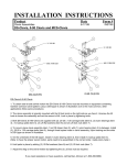
The Getting Started With Insight Dialog
Use the Getting Started With Insight dialog (shown in Figure 2-1) to open a project right
after you start Insight. Insight displays project options in the list on the left-hand side of
the dialog.
12
Chapter 2: Getting Started
13
Figure 2-1: Getting Started With Insight Dialog
Note Select the “Don’t Show This Dialog Again” option if you don’t want the Getting
Started With Insight dialog to appear the next time you start Insight.
Hint The first time you start Insight, you might want to open an example project. Example
projects contain data (listed in the Data Manager window), visualizations (displayed
in the Visualization window), and styles. Opening an example project will give you a
feel for what an Insight project looks like and how it works.
Select a project in one of the following ways:
• Click on one of the listed projects. By default, the dialog displays the three most-recently
saved projects. Click “OK” to confirm your selection and open the project.
• If the desired project is not listed, select “Other Project...” to open a file selection dialog.
Select a project file (a file with an .ipj extension) and click “OK”.
• To open a new project, select “New Project” and click “OK”. Insight automatically opens
the Select Data to Import Dialog, allowing you to import data into your new project file.
After you select a project, the Visualization window appears on the screen. The Data
Manager window also may appear (if the project was saved with the Data Manager
window open).
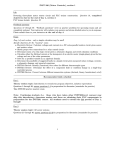
The Select Data To Import Dialog
Use the Select Data to Import dialog (shown in Figure 2-2) to import data into a new
project. You can import the following types of data:
• Files of “known” file types. By default, Insight “knows” about several different standard
image file formats (TIFF, JPEG, etc.). File formats are also “known” if a File PlugIn has
Using Insight
Starting The Insight Application
14
Chapter 2: Getting Started
been created to read the file format and placed in the PlugIns path. Some File PlugIns are
included with Insight, such as one to read binary data files with the extension .dat.
• Data stored in ASCII format files.
• IDL variables, created within the current IDL session.
Figure 2-2: Select Data to Import Dialog
File
To import a file with a known format, click “File...”. This opens an operating system native
file selection dialog. Select your file and click “OK”. If Insight does not recognize the file
extension of your file, it will present you with a list of supported file formats in the Select
File Format for Import dialog (see “Import File Menu Option” on page 36). If your file is
one of the supported types, select the file type and click “OK”.
If your file is one of the supported types, select the file type and click “OK”. If it is an ASCII
file format that isn’t supported yet, select “Define and Read ASCII...”. Otherwise, you will
need to either convert it to a supported type or create an Insight “File PlugIn” to read the
file. For more information, see “Import File Menu Option” on page 21, “Import File As
Menu Option” on page 21, or“File PlugIns” on page 206.
IDL Variables
To import an IDL Variable, click “IDL Variable...”. This opens the Import IDL Variables
dialog. Any variables that have been created in the current IDL session will be listed in the
dialog. Select the variables you wish to import and click “OK”. (You can also use IDL
commands to place IDL variables into Insight. See “INSPUT” on page 194 for details.)
After selecting files and/or IDL variables as desired, click “OK” in the Select Data to
Import dialog.
Starting The Insight Application
Using Insight
Chapter 2: Getting Started
15
Note Select the “Don’t Show This Dialog Again” option if you don’t want the Select Data
to Import dialog to appear the next time you start Insight with a new project.
You can import data into Insight at any time by
selecting “Import File...”, “Import File As...”, or
“Import IDL Variables...” from the Insight File menu.
If a duplicate file name exits, you will be prompted
with a Duplicate Data Name dialog. Select one of the
three options from the dialog.
Sharing Data Among Projects
Insight associates data imported during a session
only with the current project. If you want to use the
same data in other projects, you have a few options:
• You can use the Organizer to copy Insight data between projects. See the “Organizer” on
page 71.
• You can export data in a file format recognized by Insight. Then you can import the data
into another Insight project using that project’s import menu options.
Note You can import or export a file with a file format other than standard IDL formats
by writing a File PlugIn that handles the desired file format. See “File PlugIns” on page
206.
• You can use the “Save Project As...” menu option to save the project with a new project
name. The additional project will contain the same data as the original. See “Save Project
As Menu Option” on page 20.
• You can use the IDL routine INSGET to convert Insight data items into IDL variables, and
the INSPUT routine to convert IDL variables into Insight data items. See “INSPUT” on
page 194 and “INSGET” on page 191.
After Opening a Project
After you have selected a project to open or imported data into a new projects, the Insight
Visualization window associated with the selected project appears. For a description of
this window, see “The Visualization Window” on page 50. This is the project’s main
window and your primary working area. In this window, you will save changes to the
project, open additional projects, close the current project, and exit Insight. Using the
Visualization window’s menu and toolbar options, you can work with data in a variety of
ways and navigate to all components of the project, including the Data Manager window.
If you have opened an existing or example project, the Data Manager window also may
appear, depending on the project. Insight lists all project data in the Data Manager
window. For a description of the Data Manager window and to find out how to work with
data items, see “Working With Data” on page 29.
Using Insight
Starting The Insight Application
16
Chapter 2: Getting Started
Note At the start of a new session, you might want to set your Insight Preferences. See
“Preferences Menu Option” on page 22 or “Setting Insight Preferences” on page 22
to find out how.
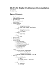
The Insight Interface
This section describes how to work with Insight’s windows, dialogs, and other interface
features. The main Insight interface screen is shown in Figure 2-3.
Figure 2-3: The Insight Interface: the main windo
demonstrating several visualizations.
Note The figures in this manual depict Motif, Microsoft Windows, and Macintosh windows
and dialogs. The dialogs and windows for all three systems operate in a similar
fashion. For more detail on using windows and dialogs for your operating system, see
your system user’s manual.
The Insight Interface
Using Insight
Chapter 2: Getting Started
17
Standard Insight Dialog Buttons
Several buttons appear in all (or most) Insight dialogs. Since buttons look different on
each platform, your buttons may not look like the examples shown in this manual.
However, they operate the same whenever they appear in Insight.
OK
Clicking “OK” permanently carries out an action, or actions, or saves modifications
specified in the dialog and closes the dialog. In Analyze dialogs, clicking “OK” also
generates or replaces a data item (or its value), which is stored in the Data Manager.
Help
Clicking “Help” opens Insight’s Online Help system to get information on the dialog and
its components.
Apply
The Apply button appears on some dialogs. Clicking “Apply” carries out an action on a
“trial” basis. This option is helpful when you want to “try out” various options before
making them “permanent.” You can click “Apply” as many times as you wish. When
you’re ready to make “permanent” data or visualization changes, click “OK”.
Cancel
Clicking “Cancel” cancels any modifications you’ve entered (or applied) and closes the
dialog.
More >>
Clicking More >> expands the dialog, providing additional dialog options.
<< Less
Clicking << Less closes the expanded section of the dialog that appeared when you
clicked More >>.
Entering File Paths
Selecting or saving files sometimes requires entering file paths in a dialog’s text field. Each
platform requires paths to be entered in a different way. For more detail on how to enter
paths on your operating system, see your system user’s manual.
Data Browsers
A number of Insight dialogs include “Browse...” buttons. Clicking “Browse...” opens an
Insight data browser, which allows you to select one (or sometimes several) Insight data
items for use in the current operation. When you click the browser’s “OK” button, Insight
uses the data as if you had provided the data name yourself.
Standard Insight Dialogs
A number of dialogs are used in multiple places in Insight. This section describes these
general purpose dialogs.
Using Insight
The Insight Interface
18
Chapter 2: Getting Started
Project Browser Dialog
If more than one project is open, this dialog will open to let you choose which project to
interact with (e.g., to import data into with INSPUT, or export data out of with INSGET).
To select a project, click on its name and hit the OK button, or simply double-click on the
name.
Note This dialog will not appear if Insight already knows which project you are interacting
with, e.g., if you are using a menu option on a specific project.
Data Browser Dialog
This dialog lets you choose one or more data items from the current project. In some
cases you will only be permitted to choose one item (such as in Analysis dialogs and the
Formulator); in others (like from INSGET) you can choose multiple items, and will have
the following additional buttons:
• All - Select all data items.
• None - Deselect all data items.
Double-clicking on a data item does an implicit "OK".
Note The choices shown in the browser are not necessarily all of the data items in the
project’s Data Manager, e.g., if only vectors are appropriate for the given situation, all
other data will have been filtered out.
Import IDL Variables Dialog
This dialog lets you choose variables from the IDL command line to import into Insight.
Double-clicking on a variable does an implicit "OK".
• All - Select all variables.
• None - Deselect all variables.
Duplicate Data Name Dialog
This dialog lets you choose what to do if a resultant data name of some action is already
in use by another data item in the project. In addition to canceling the action with the
Cancel button, you will have the following options:
• Replace the Data Item’s Value - Replaces the value of an existing data item of the same
name. This will result in dynamic updating of any current uses of that item, where possible.
For example, a visualization would automatically attempt to redraw using the new value.
• Replace the Data Item - Replaces the data item, i.e., the old data item will be deleted and
a new one will be created. Future use of the old item will no longer be possible. For
example, if an old item was being visualized, you would loose the ability to edit its
properties.
• Use Unique Name "XYZ" - The unique (unused) name displayed will be given to the new
data item.
The Insight Interface
Using Insight
Chapter 2: Getting Started
19
Duplicate Color Table Name Dialog
This dialog lets you choose what to do if a resultant color table name from some action is
already used by a color table in the project’s Color Manager. In addition to canceling the
action with the Cancel button, you will have the following options:
• Replace the Color Table’s Value - The existing color table will be replaced by a new one
(i.e., the old table will be deleted and a new one created).
• Replace Color Table - The value of the existing color table will be replaced. This will cause
dynamic updating to occur for any current uses, e.g., an image visualization would update
to reflect the new value.
• Use Unique Name "XYZ" - The unique (unused) name displayed will be given to the new
color table.
Managing Projects: The File Menu
Insight groups project management options in the File menu
of the Visualization window. Using the File menu, you can
open projects, save the current project, import data files,
export visualizations and windows, import IDL variables,
print the contents of the Visualization window, specify page
set up, open the Data Manager window, set preferences, and
exit the Insight application.
Note Many menu items in the Visualization window menus are
also accessible from the visualization toolbar. See “Insight
Toolbar” on page 51 for details.
New Project Menu Option
Select “New Project” from the File menu to create a new
Insight project. A new Visualization window will open.
New projects take on the characteristics of a template file named insight22.ipj
(.insight22.ipj on Unix systems), where “22” refers to the version
number of Insight (this is Version 2.2). You can use the template file to ensure that
data and styles (combinations of characteristics that define how individual visualization
elements appear) you want to appear in every project are included when you open a new
project.
Template files are similar in content to other project files, but have a special name,
location, and internal format. Any project file may be used as the template; simply give it
the appropriate name and location. If necessary, Insight will convert it to the proper
format and back up the original file with extension ibk.
On Windows and Macintosh systems, the template file is stored in the hook subdirectory
of the IDL lib directory. On Unix and VMS systems, the template file is stored in your
home directory.
Using Insight
Managing Projects: The File Menu
20
Chapter 2: Getting Started
If you alter or replace the insight22.ipj file, all new projects you create from then on
will take on the characteristics of the new template file.
Note Template files for Insight Version 1.0 were named insight.ipj. Old template files
existing in home directories will remain untouched to permit uninterrupted use of
previous versions of Insight.
Note If a regular project file from a previous version of Insight is opened and then saved,
it will automatically be converted to the new format. The original file will be backed
up with extension i##, where ## is the Insight version number without the decimal
point (e.g., i10 for Version 1.0).
Open Project Menu Option
Select “Open Project...” to open a file selection dialog that displays a list of existing Insight
projects (designated by the .ipj extension). Select a project in this dialog and click “OK”.
Close Project Menu Option
Select “Close Project” to close the current Insight project if you have more than one
project open. You will be prompted to save any changes to the file. All data imported into
a project will remain associated with a saved project. The next time you open the project,
it will appear as it did when you closed it. For example, if both the Visualization window
and the Data Manager window are open when you saved and closed, the next time you
open the project, both windows will be opened.
Note If you have only one project open, this option is not available. Use the “Exit” menu
option instead.
Save Project Menu Option
Select “Save Project” to save a new project or save changes to an existing project.
• When you are saving changes to an existing project, selecting the “Save” option simply
saves the changes.
• When you are saving a new project, selecting the “Save” option opens a file selection dialog
that allows you to name the project and select a directory in which the new project should
be saved. Project files should be saved with an .ipj file extension.
Save Project As Menu Option
Select “Save Project As...” to open a file selection dialog that allows you to name (or
rename) the project and select a directory in which the project should be saved. Project
files should be saved with an .ipj file extension.
Export Menu Option
Select “Export...” to export a visualization or window. When you choose the
“Visualization” or “Window” submenu, a dialog will pop up that allows you to name (or
rename) the exported file and set various attributes of the file. The exported file will have
Managing Projects: The File Menu
Using Insight
Chapter 2: Getting Started
21
the extension .gif, .jpg, .bmp, etc. For more information, see “Export File Menu
Option” on page 34.
Import File Menu Option
Select “Import File...” to import a data file. A file selection dialog opens; select the file you
wish to import and click “OK”. If Insight recognizes the file extension (.gif, .jpg, etc.),
it will automatically import the file. If it does not recognize the file extension, it will open
the Select File Format for Import dialog, allowing you to choose a file format. For more
information on importing files, see “Import File Menu Option” on page 36.
Note You can import a file with a file format other than standard IDL formats by writing
a File PlugIn that handles the desired file format. See “File PlugIns” on page 206. Once
you have added a File PlugIn to Insight that complies with the PlugIn guidelines,
Insight will recognize the file format and add it to the list of available file formats.
Import File As Menu Option
Select “Import File As...” to import a data file. The only difference between this option
and “Import File” is that choosing “Import File As...” will always prompt you with the
Select File Format for Import dialog.
Import IDL Variable Menu Option
Select “Import IDL Variables...” to open the Import IDL Variables dialog, which allows
you to import one or more IDL variables into the project. Any variables that have been
created in the current IDL session will be listed in the dialog. Select the variables you wish
to import and click “OK”. (You can also use IDL commands to place IDL variables into
Insight. See “INSPUT” on page 194 for details.)
Print Menu Option
Select “Print” to open an operating-system native Printer Setup dialog which allows you
to print the contents of the Visualization window. Settings in this dialog depend on the
printer driver installed on your system.
Note See “Preferences Dialog: General” on page 22 for information on printing preferences.
Page Setup Menu Option
Select “Page Setup” to open an operating-system native Page Setup dialog, which allows
you to specify how the page should appear when printed. Settings in this dialog depend
on the printer driver installed on your system (Mac only).
Data Manager Menu Option
Select “Data Manger...” to open the Data Manager window. The Data Manager window
displays the names and attributes of available data in the project. For a description of the
Data Manger, see “Working With Data” on page 29.
Using Insight
Managing Projects: The File Menu
22
Chapter 2: Getting Started
Preferences Menu Option
Select “Preferences...” to open the Preferences dialog, which allows you to specify settings
that Insight retains from session to session. Use this dialog to customize general Insight
features, menu display, and specify the Preferences file and PlugIns directory. When you
select a category from the Category droplist, the unique options associated with that
category appear. See “Setting Insight Preferences” on page 22 for help using the
Preference dialogs.
Exit Menu Option
Select “Exit” to exit the Insight application. You will be prompted to save changes to all
any open projects.
Caution Do not exit IDL before exiting Insight. If you do this, changes you’ve made to open
projects may be lost.
Other Visualization Window Menus
The Visualization window is described in Chapter 4, “Visualizing Data”. Chapter 5,
“Working With Visualizations”, describes the Edit menu. Chapter 4, “Visualizing Data”,
describes the Visualize menu and View menu. Chapter 6, “Analyzing Data”, describes the
Analyze menu. The Help menu is described in “Getting Help” on page 27.
Setting Insight Preferences
This section describes categories and options in the Preferences dialog, which opens
when you select “Preferences...” from the File menu. Insight preferences are stored in a file
named insight22.prf (or .insight22.prf, on Unix systems) in the same directory
as the insight22.ipj template file.
Note Preference files for Insight Version 1.0 were named insight.prf. Old preference files
existing in home directories will remain untouched to permit uninterrupted use of
previous versions of Insight.
Preferences Dialog: General
Select the “General Customization” option from the Category droplist to specify general
preferences. The General Customization options (shown in Figure 2-4) appear.
Show Startup Dialogs
From the “Show Startup Dialogs” panel, select dialogs you want to see every time you
start Insight. For example, if you want the Getting Started dialog to appear every time you
start Insight, select the “Getting Started” option.
Note If you specify a project file name via the PROJECT_FILE keyword when you start
Insight, the “Getting Started” dialog will not be displayed even if you have set the
preference to show it.
Other Visualization Window Menus
Using Insight
Chapter 2: Getting Started
23
Figure 2-4: Preferences Dialog with General
Customization Options
Print Scaling
From the “Print Scaling Options” panel, select “Fill page”, “Aspect ratio” or “None”. These
options describe how visualizations in the window will correspond to the printed page.
• Select “Fill page” to restrict or expand the contents of the Visualization window to the
paper size specified for printing.
• Select “Aspect ratio” to fill the page with all the visualizations and maintaining the aspect
ratio. Insight must scale the window contents which diminishes image accuracy.
• Select “None” so that the contents of the Visualization window appear on paper just as in
the window. The visualizations are not sized to fill the page. If they are larger than the page
size, the visualizations will be clipped.
Interactive Drag Speed
From the “Interactive Drag Speed” panel, select “High”, “Medium”, or “Low”
visualization drag speed. The higher the speed, the lower the drawing quality of the
visualization while dragging. This setting does not affect the quality of the visualization
when you are not moving it interactively with the mouse.
Hide Static Views Checkbox
When “Hide Static Views” is selected, visualizations that are not being manipulated will
not be drawn during the manipulation.
Using Insight
Setting Insight Preferences
24
Chapter 2: Getting Started
Instance Drawing/Renderer Buttons
Instance Drawing allows Insight to store the unchanging portion of the visualization and
only redraw the dynamic (changing) graphics. Because of overhead involved in creating
the instance, this technique is more effective with complex visualizations. When using
software rendering, instancing is almost always worthwhile. If your system uses hardware
rendering, you may wish to leave Instance Drawing unchecked.
You may want to experiment with software rendering even if your system supports
hardware rendering; in many cases, Insight will run faster using software rendering and
instance drawing than using the operating system’s native rendering methods.
The "Default" option for Rendering means to use the rendering option specified in the
IDE (IDL Development Environment); if the IDE is not running, however, the default is
hardware rendering. For more information, see “Hardware vs. Software Rendering” in
the Objects and Object Graphics manual.
The "Default" option for Instance Drawing means to turn on instancing if and only if
software rendering is on. For more information, see "Instancing" in the Objects and Object
Graphics manual.
Startup Color Mode
Select either the “True Color” or “Indexed Colors” option. A True Color image contains
the R,G,B values of your data. An Indexed Color image contains indexes into a color table,
which contains the R,G,B information.
Reserved Indexed Colors Options
Move the “Reserved Indexed Colors” slider to the desired number of reserved colors (1
through 256). This option works only when you’re running Insight in Indexed Color
mode. (See “INSIGHT” on page 189 for additional information on starting Insight in
different color modes.)
Selection Visual Options
Adjust the line thickness, style, and color of the lines used to highlight a selected
visualization element using the controls in this section of the dialog. Select the “Bring to
Front” checkbox to bring the particular visualization to the front of all the others.
Save Project File Compressed Checkbox
Check this box so that normal (non-template) project files will be saved in compressed
format.
When you have finished selecting options, you can select another category from the
“Category” droplist to continue setting preferences. When you have finished setting
preferences in all desired categories, click “OK”.
Preferences Dialog: Clipboard
Select the “Clipboard Customization” option from the Category droplist to specify
clipboard preferences. The Clipboard Customization options (shown in Figure 2-5)
appear.
Setting Insight Preferences
Using Insight
Chapter 2: Getting Started
25
Figure 2-5: Preferences Dialog for Clipboard
Customization
Quality
The rendering quality at which graphics are drawn to the clipboard. The default is High.
Resolution Factor
The resolution of the graphics drawn to the clipboard as compared to screen resolution
(i.e., 1/2 means the clipboard has half the resolution as the screen). The default is 1.
Preferences Dialog: Menu Display
Select the “Menu Customization” option from the Category droplist to specify menu
preferences. The Menu Customization options (shown in Figure 2-6) appear. Select
“Visualization Window” or “Data Window” from the “Menubar of ” droplist to select
menubar options for one window or the other.
To show or hide specific menu options, select or unselect the options in the scrolling list.
To show all menu options in the Visualization or Data Manager window, click the “Show
All” button. Your changes will take effect the next time you start Insight.
When you have finished selecting options, click “OK”. The dialog closes and a Question
dialog appears giving you the option to restart Insight immediately. For these preference
changes to take effect, you must restart the Insight application.
Preferences Dialog: PlugIns Path
Select the “PlugIns Customization” option from the Category droplist to specify the path
where Insight should search for PlugIns. The PlugIns Customization options (shown in
Figure 2-5) appear. By default, this path is set to the plugins subdirectory of the
Using Insight
Setting Insight Preferences
26
Chapter 2: Getting Started
Figure 2-6: Preferences Dialog with Menu
Customization Options
insight subdirectory of the examples directory in the IDL distribution. A number of
example PlugIns are included in this directory.
Figure
2-7:Preferences
Dialog
forSpecifying
the
PlugIns Path
• Click “Add” to add a directory to the list.
• Click “Remove” to remove a directory from the list.
Setting Insight Preferences
Using Insight
Chapter 2: Getting Started
27
• Click “Move Up” to move a directory up one in the list.
• Click “Move Down” to move a directory down one in the list.
Insight will search for all .pro and .sav files in the directories from top to bottom in the
list. If both a .pro and a .sav file exist for the same PlugIn in a given directory, the .pro
file will be used. If a given PlugIn exists in multiple directories, it will be ignored in all but
the first directory in which it is located.
Note All of the .pro and .sav files in the PlugIns path must be PlugIns.
Preferences Dialog: Preference File
Select the “Preference” option from the Category droplist to specify the file to which
Preferences will be written. The Preferences Customization options (shown in Figure 28) appear.
Figure 2-8:
Preferences Dialog for Specifying the
Preference File
Select the Preference file in one of the following ways:
• Enter a filename in the “Preference File” text field; or
• Click “Browse” to open a file selection dialog. Select a file in the normal way.
Getting Help
Insight provides several ways to get information on various Insight topics. You can access
the online help system by:
• clicking the “Help” button in dialogs
Using Insight
Getting Help
28
Chapter 2: Getting Started
• selecting an option from Insight’s Help menu
• entering ? at the IDL command prompt
You also can refer to the printed Insight and/or IDL documentation.
IDL Help
Select “IDL Help” to open the IDL online help files. IDL’s
Online Help system gives you access to all volumes of the IDL
documentation set in electronic, hypertext-linked format.
Insight Help
Select this option to open the Insight online help files.
The Visualization Window Menu Option
This option appears when you’re working in the Visualization window. Select this option
to get information on Insight’s Visualization window.
The Data Manager Window Menu Option
This option appears when you’re working in the Data Manager window. Select this option
to get information on Insight’s Data Manager window.
About Insight
Select this option to open a dialog which displays the Insight and IDL versions you are
using. Click “OK” to close the dialog.
Getting Help
Using Insight
Chapter 3
Working With Data
The following topics are covered in this chapter:
The Data Manager Window .................. 30
The Data Manager Window Menubar ... 30
Data Attributes Overview ...................... 31
Saving in the Data Manager Window.... 33
Importing and Exporting Data ............. 34
Reading ASCII Format Files .................. 37
Editing and Creating Data ................... 37
Viewing Data ....................................... 42
Conditioning Data ............................... 44
29
30
Chapter 3: Working With Data
This chapter introduces Insight’s Data Manager window and menu options and describes
data attributes. You will learn how to use the Data Manager window’s File, Edit,
Condition, and View menus to work with data in various ways including importing,
exporting, creating, and conditioning.
The Data Manager Window
The Data Manager window (shown in Figure 3-1) is your view of the Insight data area
associated with the Insight project. Basically, it’s a list of data items with specific
information about each, called attributes. To open the Data Manager window, select the
“Data Manager...” option from the File Menu in the Visualization window. As a shortcut,
you can click the “Data Manager” button in the Visualization Toolbar (the button
displays the letters “DM”). The Data Manager window displays a table listing the
attributes of data items which have been imported or created for the project. Insight lists
data names in row headers with attributes displayed in columns to the right.
DataManager
menubar
of options
Attribute
Columns
(To sort by
specifi
c
attribute, c
the desired
column
header
.)
Data Names
listed in row
headers
Figure 3-1: Data Manager Window
DataAttribute
(listed in
columnstothe
right of each
data name)
The Data Manager Window Menubar
The menubar across the top of the Data Manager window has five main menus: File, Edit,
View, Condition, and Help. When you select a menu option that is followed by an ellipsis
(...), Insight opens a dialog or window so you can enter more information or select
options before performing an operation. The operations you can perform include:
• customizing your view of data and attributes,
• creating, importing, and exporting data,
• conditioning existing data,
• viewing and modifying attributes of existing data,
• viewing data values.
The Data Manager Window
Using Insight
Chapter 3: Working With Data
31
Data Attributes Overview
Insight organizes the information describing data as a set of attributes. Examples of
attributes are name, classification, type, dimensions, elements, and description. This
section describes the data attributes used by the Insight Data Manager.
Note To modify one or more attributes of a data item, select the data item from the Data
Manager’s table, then select “Attributes...” from the Edit menu in the Data Manager
window. To view the value of selected data, select “Value...” from the Edit menu of
the Data Manager window.
When you create new data items within Insight, you assign the attributes explicitly. For
example, when you select “Create Data” from the Edit menu in the Data Manager
window, a dialog (shown in Figure 3-2) allows you to specify attributes for your data.
When you import data, Insight determines most data attributes for you.
Figure 3-2: Data Attributes Dialog
Data Attributes
This section describes the attributes associated with data.
Name
This attribute contains the name of the data. Data created in Insight has a name assigned
by you or by Insight. Names must start with a letter but can include letters, numbers,
underscore characters, or single spaces.
Note If you do not choose to name your data, Insight uniquely names new data based on
data type and sequence.
Using Insight
Data Attributes Overview
32
Chapter 3: Working With Data
Classification
This attribute displays the classification of the data. Insight classifies data as a type of
variable: Scalar, Vector (a one-dimensional array), Arrays (2D through 8D), or Image.
Type
This attribute contains the type of data. Each data item has one of the following data
types:
Byte
Unsigned integers from 0 to 255.
Integer
Integers from -32768 to +32767.
Long
Integers from -231 to 231 -1.
Float
32-bit, single-precision, floating-point number in
the range of ±1038(IEEE)
Double Float
64-bit, double-precision, floating-point number in
the range of ±10308(IEEE)
Complex
A real, imaginary pair of floating-point numbers.
Double Complex
A [real, imaginary] pair of double-precision numbers.
String
A sequence of 0 to 32,767 characters.
Table 3-1: Insight Data Types
Dimensions
This attribute contains the number of elements in each dimension of the data. The
column contains one number for a vector and two to eight numbers for an array. For
example, the “Dimensions” column contains “60, 60” for a two-dimensional array with
60 elements by 60 elements.
Elements
This attribute contains the total number of elements in the data item. Basically, the total
is the product of all of its dimensions. For example, the “Elements” column will contain
the number “3600” for a two-dimensional array with 60 elements in one dimension and
60 in the other.
Description
This attribute contains the description of the data item. If the data was generated in an
Analyze dialog, this field also lists the options you selected in that dialog.
Modification Time
This attribute contains the date and time of the last modification.
Source
This attribute contains the source of the data. The source is one of:
Data Attributes Overview
Using Insight
Chapter 3: Working With Data
33
• “Project <filename>” if the data item was copied via the Organizer.
• “File <filename>” if the data item was imported into Insight from a file.
• “Insight Command” if the data came through an argument to the INSIGHT command.
• “Analysis <modulename>” if the data item was created by an Analysis module.
• “InsPut” if you used the INSPUT function from the IDL command line to import the data.
• “Insight Create” if you created the item in the Data Manager window.
• “Formulator” if you created the item with the Formulator.
Size
This attribute contains the number of bytes in the data.
Value
This displays the value of the selected data.
Min
This is the minimum value of the data.
Max
This is the maximum value of the data.
Order
This option contains the display order for image data.
Color Table
This option contains the name of the color table for image data.
Format
This allows the user to enter a format string (minus parentheses) which is then used as
the default format for displaying data values textually.
Saving in the Data Manager Window
Data is just another part of the Insight project; select “Save Project” or “Save Project As...”
from the Visualization window’s File menu to save newly created or imported data items
Hint As a shortcut you can use the Save button from the Insight Toolbar, which is described
on page 51.
Using Insight
Saving in the Data Manager Window
34
Chapter 3: Working With Data
Importing and Exporting Data
Insight groups the Data Manager window’s data input and
output options in the Data Manager File menu. Using this menu,
you can import and export data files, import IDL variables, and
close the Data Manager window.
Note You also can import files and IDL variables using import
menu options in the File menu in the Visualization window.
Export File Menu Option
After choosing a file from the Data Manager, select “Export File” to export the file as one
of the formats listed (JPEG, TIFF, GIF, etc.). A file Export dialog will open.
Note The availability of the following options depends on the file type chosen.
Figure 3-3: File Export Dialog
File
Enter the file name or use the Browse button to select the file name for export.
Note Be sure to include the proper extension on the file name. The extensions
(.tif,.jpg,.gif, etc.) are not automatically included in the file name.
Image Dimensions
Enter the X and Y dimensions of the export image. Use the droplist to select either pixels,
inches, or centimeters.
Resolution
Enter the resolution of the image.
Importing and Exporting Data
Using Insight
Chapter 3: Working With Data
35
Note This option is not available if the image dimensions are in pixels.
Type Droplist
Select the export file type from this droplist. File types supported include:
BMP - Windows Bitmap
DAT - Structured Binary
GIF - Graphics Interchange Format
HDF - Hierarchical Data Format
JPEG, JPG - Joint Photographic Experts
Group
PICT - Macintosh Picture Format
PPM, PGM - PPM or PGM Format
SRF, SUN, RAST - Sun Raster File
TIFF, TIF - Tagged Image File Format
XWD - X Windows Dump
VRML - Virtual Reality Modeling Language (Note: This format is not available when
exporting with the Data Manager. It is only available when exporting using Insight’s main
“Export Menu Option” on page 20.)
NOTE: The following options apply only to the JPEG (or JPG) format.
Order Droplist
Select the order in which the export file will be written: “Top to Bottom” or “Bottom to
Top”.
Progressive Scans Droplist
Select “Yes” to write the image as a series of scans of increasing quality, or “No” to write
the image all at once.
Quality
Enter the quality of the export file. The quality scale ranges from 0 (bad) to 100
(excellent). The default is 75 which is considered very good quality.
Note You can export a file with a file format other than standard IDL formats by writing a
File PlugIn that handles the desired file format. See “File PlugIns” on page 206. Once
you have added a File PlugIn to Insight, it will be contained in the list of available file
formats.
For more information about exporting files, see WRITE_JPEG and other
WRITE_(TYPE) functions in the IDL Reference Guide.
Using Insight
Importing and Exporting Data
36
Chapter 3: Working With Data
Import File Menu Option
Select “Import File” to import an data file (TIFF, JPEG, etc.). A file selection dialog opens;
select the file you wish to import and click “OK”. If Insight recognizes the file extension
(.gif, .jpg, etc.), it will automatically import the file. If it does not recognize the file
extension (or if there is more than one method for opening files of the specified type), it
will open the Select File Format for Import dialog, allowing you to choose a file format.
Figure 3-4: Select File Format for Import Dial
The various file types should be familiar to most users with the possible exception of
the.hdf format, which stands for “Hierarchical Data Format” or HDF. For more
information about HDF, see the Scientific Data Formats manual.
If you select “Define and Read ASCII...” from the Select File Format for Import dialog,
Insight will allow you to interactively define the format of an ASCII data file and then read
the file. The ASCII file reader is described in “Reading ASCII Format Files” on page 37.
Note You can import a file with a file format other than standard IDL formats by writing
a File PlugIn that handles the desired file format. See “File PlugIns” on page 206. Once
you have added a File PlugIn to Insight, it will be contained in the list of available file
formats.
When you import data, Insight places the data in the project’s data area. You can view the
name and other attributes of the data in the Data Manager window.
Import File As Menu Option
Select “Import File As...” to import a data file. The only difference between this option
and “Import File” is that choosing “Import File As...” will always prompt you with the
Importing and Exporting Data
Using Insight
Chapter 3: Working With Data
37
Select File Format for Import dialog, even when the file extension matches one of the
extensions that Insight knows about.
Import IDL Variables Menu Option
Select “Import IDL Variables...” to open the Import IDL Variables dialog, which allows
you to import one or more IDL variables from the IDL MAIN level into the project.
Close Menu Option
Select this option to close the Data Manager window.
Reading ASCII Format Files
Selecting the "Define and Read ASCII..."
option in the Select File Format for
Import dialog launches an interface
which allows you to define the format of
your ASCII file. It then reads your data
into Insight. (See ASCII_TEMPLATE and
READ_ASCII in the IDL Reference Guide.)
After the data is successfully read, a native file browser will let you save the ASCII file
description, or "template", as a File PlugIn. If you have multiple files of the same format,
this will enable you to read them into Insight without having to redefine the format each
time.
The PlugIn should be put into a directory of your PlugIns Path, and be saved with a .pro
extension. Since the PlugIn is IDL code, you may customize it, if desired (see “File
PlugIns” on page 206 for further information).
If you do not want a File PlugIn created, simply cancel from the file browser.
See “Importing ASCII Data” on page 184 for a tutorial on using Insight’s ASCII reading
capabilities.
Editing and Creating Data
The Data Manager’s Edit menu provides options for working with
data, including viewing and modifying data attributes, viewing
data values, and creating new data.
Undo Menu Option
Select “Undo” to reverse the most recent action taken. You can
“undo” the following actions: delete, duplicate, create scalar, create
array, attribute changes, and data conditioning operations. In general, you have the
option to undo an action until you take the next action.
Using Insight
Reading ASCII Format Files
38
Chapter 3: Working With Data
Redo Menu Option
Select this option to reverse the previous “Undo” action. You can select this option after
selecting the Undo option.
Delete Menu Option
Select this option to remove the selected data from the project.
Duplicate Menu Option
Select this option to duplicate selected data. The duplicate data appears in the Data
Manager window with a name generated by Insight and based on the original name.
Create Data Menu Option
Select this option to access a submenu of data types you can create: “Scalar...” or “Array...”.
In IDL, data can be scalars or arrays of up to eight dimensions. For more detail on data
types, see “Type” on page 32.
Scalar
Select this option from the Create Data menu to create a
single-element variable (a scalar). The Create Scalar Data
dialog appears.
1.
To change the name, click in the “Name” text field and edit.
2.
From the “Type” droplist, select a type of scalar: Byte,
Integer, Long Integer, Float, Double Float, Complex, Double Complex, and String.
3.
Enter a value in the “Value” text field.
4.
Enter a description of the scalar in the “Description” text
field, if you wish.
5.
When you are finished, click “OK”. Insight stores the scalar and lists its attributes in the
Data Manager window.
Editing and Creating Data
Using Insight
Chapter 3: Working With Data
39
Array
Select this option from the Create Data
menu to create data with up to eight
dimensions.The Create Array Data
dialog appears.
1.
To change the name, click in the
“Name” text field and edit.
2.
From the “Type” droplist, select a type
of array: Byte, Integer, Long Integer,
Float, Double Float, Complex, Double
Complex, and String.
3.
Enter values in the “Dimensions” text
fields that correspond to the size of each
array dimension.
4.
Select “Scalar Value” or “Indexed” initialization type. If you select “Indexed”, the array
will be set to zero for the first element and incremental values for the rest of the array. If
you select “Scalar Value”, each element of the array will be initialized with the value you
enter in the “Initial Value” text field.
5.
If you selected “Scalar Value” type, enter a number (or value) in the “Initial Value” text
field.
6.
Enter a description in the “Description” text field, if you wish.
7.
When you are finished, click “OK”. Insight stores the array in the project.
To view the data, see the Data Manager window.
Attributes Menu Option
Select this option to open the Data Attributes dialog, which allows you to view and edit
attributes of data selected in the Data Manager window.
Using Insight
Editing and Creating Data
40
Chapter 3: Working With Data
The Scalar Data Attributes dialog
Attributes listed in the Scalar Attributes
dialog include name, classification,
type, dimensions, elements, size, value,
minimum, maximum, source,
description, and last modification date
and time.
1.
To change the name, click in the
“Name” text field and edit.
2.
To modify the value, click in the “Value”
text field and edit.
3.
To add or change a description, click in
the “Description” text field and add or
edit.
4.
Use the “Format” field to enter a format
string (minus parenthesis) which will be used as the default format for displaying data
values textually. See format codes in Using IDL for more information.
5.
When you are finished, click “OK” to change the attributes for the data and close the
dialog.
The Array Data Attributes dialog
Attributes listed in the Array Attributes
dialog include name, classification,
type, dimensions, elements, size,
minimum, maximum, source,
description, and last modification date
and time.
1.
To change the name, click in the
“Name” text field and edit.
2.
To view the value of an Array, see “Value
Menu Option” on page 42.
3.
To add or change a description, click in
the “Description” text field and add or
edit.
4.
Use the “Format” field to enter a format
string (minus parenthesis) which will be used as the default format for displaying data
values textually. See format codes in Using IDL for more information.
5.
When you are finished, click “OK” to change the attributes for the data and close the
dialog.
Editing and Creating Data
Using Insight
Chapter 3: Working With Data
41
The Image Data Attributes dialog
Attributes listed in the Image Attributes
dialog include name, classification,
type, dimensions, elements, size,
minimum, maximum, source, display
order, true color, color table,
description, and last modification date
and time.
1.
To change the name, click in the
“Name” text field and edit.
2.
Select “Bottom Up”, “Top Down”, or
“Not Set” to specify the order in which
the image should be written to the
screen. If you select “Not Set”, Insight
determines the order based on the image’s visualization properties.
3.
From the scrolling list, select the color table desired. Only indexed color images use color
tables. For more information, see “Color Tables” in Chapter 12 of Using IDL.
4.
Use the “Format” field to enter a format string (minus parenthesis) which will be used as
the default format for displaying data values textually. See format codes in Using IDL for
more information.
5.
To modify a description, click in the “Description” text field and edit.
6.
When you are finished, click “OK”. Data attributes are changed and the dialog closes.
Statistics Menu Option
Select “Statistics...” to open a Statistics dialog which displays the following information
about the selected data:
Minimum: the minimum value.
Maximum: the maximum value.
Mean: the average value of a set of values.
Mean Absolute Deviation: the sum of the absolute distance of each sample element from
the population (or set of values) mean.
Median: the value in an ordered set of values below and above which there is an equal
number of values or which is the arithmetic mean of the two middle values if there is no
one middle number.
Variance: the square of the standard deviation.
Standard Deviation: the root mean square of the deviations (distances) from the
population mean.
Using Insight
Editing and Creating Data
42
Chapter 3: Working With Data
Skewness: lack of symmetry.
Kurtosis: The peakedness or flatness of the graph of a frequency distribution, especially
with respect to the concentration of values near the mean as compared with the normal
distribution.
Value Menu Option
The Scalar Value Dialog
If you have selected scalar data, the Scalar Value dialog opens. When you are finished,
click “Close”.
The Array Value Dialog
If you have selected array data, the Array Value dialog opens. Use the scroll bars to
navigate to all rows and columns in the “Dimensions” table. Choose up to two
dimensions (if applicable) to display. For example, if you select “16” in the Dim 1 column
and “*” in Dim 2 column, the table will display the values for all the rows of column 16.
Viewing Data
The Data Manager’s View menu provides options for displaying data
and attributes in the Data Manager window.
All Attributes Menu Option
Select “All Attributes” to view all attributes for all data in the Data
Manager window.
Figure 3-5: Statistics Dialog with example
statistics for Noisy Damped Sine data
Viewing Data
Using Insight
Chapter 3: Working With Data
43
Partial Attributes Menu Option
Select “Partial Attributes...” to open the Partial Attributes dialog in which you can specify
attributes you wish to view for data in the Data Manager window. Select the checkbox to
the left of each desired attribute. When you have finished, click “OK”. Insight displays the
selected attributes and hides the rest from view.
Figure 3-6: Partial Attributes Dialog
Filter Menu Option
Select “Filter” to view a submenu of options representing data
classifications. When you select one of the options, Insight displays only
data matching that classification in the Data Manager window. For
example, if you select the “Image” menu option, Insight only displays the
names and attributes of data classified as images. See “Data Attributes” on
page 31.
Sort Menu Option
Select “Sort” to view a submenu of options representing the data
attributes by which you can sort. Sort options include: classification,
dimensions, modification time, name, size, source, and type. When
you select an option, Insight sorts all data in the Data Manager
window by that attribute. For example, if you select the “By Type”
menu option, Insight sorts and displays data by type. All “Byte” data
would be listed together followed by all data items for another type.
Using Insight
Viewing Data
44
Chapter 3: Working With Data
Figure 3-7: Reformat Dialog for Vectors and Arrays (up to 8
Note You also can sort by simply clicking the desired column header in the Data Manager
window.
Conditioning Data
Use the Data Manager’s Condition menu options to reformat, resize,
reverse, sample, sort, and transpose data.
Note The difference between data conditioning and data analysis: Data
conditioning involves relatively simple operations which modify
the values of existing data items. Data analysis is typically a more
complicated process whereby multiple data items may be used
together in an algorithm to generate, replace, or modify data
items, optionally applying different parameters on a trial basis, and visualizing the
result.
Reformat Menu Option
Select “Reformat” to open the Reformat dialog in which you can view or modify the
dimensions of a selected array without changing the total number of elements. Reformat
dialog options depend on dimensionality of the selected data. The array can have one to
eight dimensions. Only the dimensions of the array are changed; the actual data remains
unmodified. For more details, see “REFORM” in the IDL Reference Guide.
Using The Reformat Dialog
1. Select data in the Data Manager window.
2.
Select the “Reformat” option from the Condition menu. The Reformat dialog opens. The
dialog displays the name of the data and the size of each dimension.
3.
Edit the “Dimension” text fields with the desired sizes.
4.
When you are finished, click “OK”.
Conditioning Data
Using Insight
Chapter 3: Working With Data
45
Resize Menu Option
Select “Resize” to open the Resize dialog which allows you to shrink or expand the size of
an array by an arbitrary amount. Insight computes intermediate data values based on the
existing data values. Resize dialog options depend on dimensionality of the selected data.
The array can have one to three dimensions. For one- and two-dimensional arrays,
Insight uses one of three methods: nearest neighbor sampling, linear interpolation, or
convolution interpolation. For three-dimensional arrays, Insight uses linear
interpolation. For more details, see “CONGRID” in the IDL Reference Guide.
Figure 3-8: Resize Dialog for 2D Arrays
Using The Resize Dialog
1. Select data in the Data Manager window.
2.
Select the “Resize” option from the Condition menu. The Resize dialog opens. The dialog
displays the name of the data and the size of each dimension.
3.
Edit the “Dimensions” text fields with the desired sizes.
4.
For one- and two dimensional data: From the “Method” panel select “Nearest Neighbor
Sampling”, “Linear Interpolation”, or “Convolution Interpolation”. Insight uses Linear
Interpolation for three-dimensional data.
• Nearest Neighbor Sampling computes an intermediate data value, called an “interpolate,”
by averaging the points immediately surrounding the location of the interpolate in all
possible directions.
• Linear Interpolation computes an intermediate data value using the points immediately
surrounding the location of the interpolate in only one direction.
Using Insight
Conditioning Data
46
Chapter 3: Working With Data
• Convolution Interpolation uses the “Cubic Convolution” algorithm.
5.
When you are finished, click “OK”. You can view the data’s new dimensions in the
“Dimensions”” column in the Data Manager window or in the Attributes dialog
Reverse Menu Option
Select “Reverse” to open the Reverse dialog in which you can reverse the order of entries
in a one to three-dimensional array. Reverse dialog options depend on dimensionality of
the selected data. For more details, see “REVERSE” in the IDL Reference Guide.
Figure 3-9: Reverse Dialog for 2D Arrays
Using The Reverse Dialog
In the dialogs for two- and three-dimensional arrays, select the dimensions to reverse.
Click “OK”.
Sample Menu Option
Select “Sample” to open the Sample dialog in which you can create a subset of a selected
array. Sample dialog options depend on dimensionality of the selected array. The array
can have one to eight dimensions. This allows you to zero in on specific features of your
data. For example, for a 10 X 10 X 10 array, you can see elements 2 through 4 in the first
dimension, 5 through 7 in the second dimension, and 1 through 8 in the third dimension.
Simply edit the “From” and “To” text fields with the desired values. Note that dimension
values must be greater than or equal to zero and less than the size of the dimension minus
one.
Sort Menu Option
Select “Sort” to open a Sort dialog in which you can sort selected vectors in ascending or
descending order. For more detail, see “SORT”, “ROTATE”, and “UNIQ” in the IDL
Reference Guide.
Using The Sort Dialog
1. Select to sort the data values in either “Ascending” or “Descending” order.
Conditioning Data
Using Insight
Chapter 3: Working With Data
47
Figure 3-10: Sample Dialog for 2D Arrays
Figure 3-11: Sort Dialog for Vectors
2.
Select the “Unique Elements” checkbox to keep repeated values out of the sort. Insight
will then sort only unique values.
Transpose Menu Option
Select “Transpose” to open a Transpose dialog which allows you to transpose an array.
The array can be one to eight dimensions. Transpose dialog options depend on
dimensionality of the selected data. For a two-dimensional array, Insight rearranges the
dimensions of the array from column major format to row major format or vice versa.
Row major format means that the linear order of the data elements proceeds from the first
element of the first row through the last element of the first row before beginning on the
second row, etc. For arrays of higher dimensionality, the Transpose dialog allows you to
specify the transposition order. For more detail, see “TRANSPOSE” in the IDL Reference
Guide.
Hint This is especially helpful if you wish to use an array in the Data Manager as input to
an IDL function that expects data in row-major format. IDL always allocates and
references data in row-major format.
Using Insight
Conditioning Data
48
Chapter 3: Working With Data
Figure 3-12: Transpose Dialog for 3D Arrays
If the data has three-to eight dimensions, you can enter a permutation vector. For one dimensional data, the Transpose option converts between a row and column vector. For
two-dimensional data, the rows and columns are switched, but no permutation vector is
required.
PlugIns Menu Option
Select “Plugins” to view a submenu of Conditioning PlugIns. Selecting one of the PlugIns
displayed performs the PlugIn’s conditioning operation on the item selected in the Data
Manager window.
A PlugIn is a routine written in the IDL language. PlugIns must follow Insight’s PlugIn
conventions as described in “Extending Insight” on page 203. Conditioning PlugIns
modify the value of a selected Insight data item. You can add Conditioning PlugIns to
perform such tasks as rotating, scaling, rounding, and shifting.
Help Menu
The Data Manager Help menu provides options for getting help.
Using these options, you can access online help files and get
information on IDL and Insight. To find out how to use these
options, see “Getting Help” on page 27.
Conditioning Data
Using Insight
Chapter 4
Visualizing Data
The following topics are covered in this chapter:
What Is Visualization?............................ 50
The Visualization Window ..................... 50
The Visualize Menu ............................... 52
Line Plots .............................................. 53
Scatter Plots.......................................... 54
Histogram Plots .................................... 55
Polar Plots ........................................... 56
Contours ............................................. 58
Images ................................................ 59
Surfaces ............................................... 60
The View Menu ................................... 63
Selecting Visualizations ........................ 66
49
50
Chapter 4: Visualizing Data
This chapter describes visualization. It introduces the Insight Visualization window and
its menubar and toolbar. You will learn how to use the Visualize menu to display data and
the View menu to customize your view of data in the window.
What Is Visualization?
We use the term visualization as a catch-all to refer to a data set that has been displayed
on your computer in some format. Visualizations include plots, contours, surfaces,
images, and all of the ancillary elements that go along with them — axes, annotations, etc.
When you display data in Insight, you see it appear in the Visualization window.
Using the window’s Visualize menu options, you can display several types of
visualizations: line plots, scatter plots, histogram plots, polar plots, contours, surfaces,
and images. The graphic parts that make up a visualization — the plot or image, axes,
tickmarks, annotations, etc. — are called elements in this document. Often, each element
of a visualization has its own set of properties (location, color, width, style, etc.) and can
be customized independently of the other elements in the visualization. You can view and
modify properties using the element’s Properties dialog. See “The Properties Dialogs” on
page 74 for details on setting properties.
The Visualization Window
When you start Insight and open a new or existing Insight project, the Visualization
window appears on your screen as a viewing area with a menubar and toolbar. The
Visualization Window is shown in Figure 4-1.
The Visualization window is the primary workspace in which you visualize data. It is also
the hub from which you can navigate to:
• Analysis dialogs which allow you to analyze, generate, and modify data and visualizations,
• the Data Manager window, where Insight lists names and attributes of all existing
project data.
• other Insight projects
By default, the existing visualization is cleared from the Visualization window when a new
visualization is created. See “Retain All Visualizations” on page 65 for details on how to
alter this behavior.
What Is Visualization?
Using Insight
Chapter 4: Visualizing Data
51
Visualization
W indow
menubar of
options
Visualization
Toolbar
Viewing area
where data is
visualized
Bounding box
indicating
that
a visualization
is selected
The plotline
and the axes
are both
elements
included
inthe
visualization
A description
of
thebutton
over
which the
mouse is
positioned
appears here.
Figure 4-1: Visualization Window (shown with an example)
Insight Toolbar
The Insight Toolbar appears across the top of the Visualization window below the
menubar. The Toolbar features buttons corresponding to various menu options. When a
menu option is disabled, the corresponding toolbar button is disabled as well. When you
move the mouse over each button, the name of the button appears in the lower left-hand
corner of the Visualization window. The figure below shows the default toolbar buttons.
New
Open
Save ImportImport PrintData
Undo
Line Scatter
Histogram
PolarContour
Copy Plot Plot Plot
ProjectProjectProject
File IDL
Manager
Plot
Variable
Image
Redo
Surface
Line
Annotation
Rectangle
Annotation
Text
Annotation
Figure 4-2: Toolbar Buttons
Using Insight
The Visualization Window
52
Chapter 4: Visualizing Data
Visualization Window Menubar
The menubar across the top of the Visualization window groups Insight operations into
six main menus: File, Edit, Visualize, Analyze, View, and Help. When you select a menu
option that is followed by an ellipsis (...), Insight opens a dialog or window so you can
enter more information or select options before performing an operation.
You’ll find descriptions of Visualization window menus throughout this volume. Chapter
2, “Getting Started” describes the File menu (project management options) and Help
menu options. Chapter 5, “Working With Visualizations”, describes the Edit menu (how
to edit, annotate, and change the properties of visualizations). Chapter 6, “Analyzing
Data”, describes the Analyze menu (performing analyze operations, accessing Analysis
PlugIns, using the formulator). This chapter describes the Visualize Menu (how to display
data in the Visualization window) and View Menu (how to specify your view in of the
data in the window).
The Visualize Menu
The Visualize menu provides options for visualizing data in the
Visualization window. Using these options you can visualize line
plots, scatter plots, histogram plots, polar plots, contours, images,
and surfaces. Each option opens a dialog from which you can select
data and specify options. The data items available include data in the
project that fit the current operation. For example, data of type
“Image” are not available when creating a line plot.
Note You can also access the visualize menu options (line plot, scatter plot, histogram plot,
polar plot, contour, image, and surface) from the toolbar.
Figure 4-3: Toolbar Selections (line plot, scatter pl
histogram plot, polar plot, contour, image, and surfac
The Visualize Menu
Using Insight
Chapter 4: Visualizing Data
53
Figure 4-4: Line Plot and Line Plot Dialog
Line Plots
Select “Line Plot” to open a Line Plot dialog from which you can
select data and options for drawing a line plot in the Visualization
window. A line plot is a plot of data points with straight line segments
connecting them.
The Line Plot Dialog
Selecting the “Line Plot” option from the Visualize menu opens the
Line Plot dialog.
1.
Select one or more vectors by checking the box in the “Y” column to the left of one or
more data items in the data selection list.
If you select only the “Y” column for a data item, Insight will label the Visualization’s Y
axis with data values (the dependent data) and label the X axis with the indices of the data
item.
Optionally, select one box in the “X” column for any data item in the list. If you select an
X and a Y, Insight will plot the Y (the dependent data) as a function of the X (independent
data).
2.
From the “Plot Style” droplist, select a style. Styles determine the “look” of your visualization. For more information on styles, see “About Styles” on page 100.
Using Insight
Line Plots
54
Chapter 4: Visualizing Data
Figure 4-5: Scatter Plot and Scatter Plot Dialog
Note If you want to view more than one visualization at a time, set up the tiling scheme in
your Visualization window. Always set up the tiling scheme before doing a visualization. For more details, see “The View Menu” on page 63.
3.
When you are finished with the dialog, click “OK”. The dialog closes and Insight displays
the plot in the Visualization window. To view or modify this plot, see “Editing Visualizations: The Edit Menu” on page 68 or “Properties (Visualizations)” on page 73.
Scatter Plots
Select “Scatter Plot” to open a Scatter Plot dialog from which you can
select data and options for drawing a scatter plot in the Visualization
window. A scatter plot contains plotted symbols at data points
without connecting them.
The Scatter Plot Dialog
Selecting the “Scatter Plot” option from the Visualize menu opens the
Scatter Plot dialog.
1.
Select one or more vectors by selecting the “Y ” box to the left of one or more data items
in the data selection list.
If you select only the “Y” box for a data item, Insight will label the Visualization’s Y axis
with data values (the dependent data) and label the X axis with the indices of the data
item.
Scatter Plots
Using Insight
Chapter 4: Visualizing Data
55
Figure 4-6: Histogram Plot and Histogram Dialog
Optionally, select one “X” box for any data item in the list. If you select an X and a Y,
Insight will plot the Y (the dependent data) as a function of the X (independent data).
2.
From the “Scatter Plot Style” droplist, select a style. Styles determine the “look” of your
visualization. For more information on styles, see “About Styles” on page 100.
3.
When you are finished with the dialog, click “OK”. The dialog closes and Insight displays
the plot in the Visualization window. To view or modify this plot, see “Editing Visualizations: The Edit Menu” on page 68 or “Properties (Visualizations)” on page 73.
Histogram Plots
Select this option to open a Histogram Plot dialog from which you
can select data and options for drawing a histogram plot in the
Visualization window. A histogram plot shows horizontal and
vertical lines connecting data points.
The Histogram Dialog
Selecting the “Histogram” option from the Visualize menu opens the
Histogram dialog.
1.
Select one or more vectors by selecting the “Y ” box to the left of one or more data items
in the data selection list.
Using Insight
Histogram Plots
56
Chapter 4: Visualizing Data
Figure 4-7: Polar Plot and Polar Plot Dialog
If you select only the “Y” box for a data item, Insight will label the Visualization’s Y axis
with data values (the dependent data) and label the X axis with the indices of the data
item.
Optionally, select one “X” box for any data item in the list. If you select an X and a Y,
Insight will plot the Y (the dependent data) as a function of the X (independent data).
2.
From the “Histogram Style” droplist, select a style. Styles determine the “look” of your
visualization. For more information on styles, see “About Styles” on page 100.
3.
When you are finished with the dialog, click “OK”. The dialog closes and Insight displays
the plot in the Visualization window. To view or modify this plot, see “Editing Visualizations: The Edit Menu” on page 68 or “Properties (Visualizations)” on page 73.
Polar Plots
Select “Polar Plot” to open a Polar Plot dialog from which you can
select data and options for drawing a polar plot in the window. A
polar plot is a plot of data in the polar coordinate system (using angle
Theta and radius instead of the cartesian (x, y) coordinate system).
Polar plots display the data item in terms of angle (Theta: radians)
and distance (r: radius) from the origin (0, 0).
Polar Plots
Using Insight
Chapter 4: Visualizing Data
57
The Polar Plot Dialog
Selecting the “Polar Plot” option from the Visualize menu opens the Polar Plot dialog.
1.
Select one “T” (angle) box for any vector in the list.
2.
Select one or more vectors in the “r” (radius) box in the data selection list.
Note You can only select one “T” (angle) box, but you can select multiple “r” (radius) boxes.
The “r” vectors (dependent variables) are plotted against the “T” angle (independent
variable).
3.
From the “Polar Plot Style” droplist, select a style. Styles determine the “look” of your
visualization. For more information on styles, see “About Styles” on page 100.
4.
When you are finished with the dialog, click “OK”. The dialog closes and Insight displays
the plot in the Visualization window. To view or modify this plot, see “Editing Visualizations: The Edit Menu” on page 68 or “Properties (Visualizations)” on page 73.
Using Insight
Polar Plots
58
Chapter 4: Visualizing Data
Figure 4-8: Contour and Contour Dialog
Contours
Select “Contour” to open a Contour dialog from which you can select
a data item to display as a contour plot in the Visualization window.
The Contour Dialog
Selecting the “Contour” option from the Visualize menu opens the
Contour dialog.
Contours
1.
Select one data items by selecting the “Z” box to the left of one data
item in the data selection list. Optionally select one “X” and one “Y” box for any data item
in the list.
2.
From the “Contour Style” droplist, select a style. Styles determine the “look” of your
visualization. For more information on styles, see “About Styles” on page 100.
3.
When you are finished, click “OK”. The dialog closes and Insight displays the contour in
the Visualization window. To view or modify this surface, see “Editing Visualizations: The
Edit Menu” on page 68 or “Properties (Visualizations)” on page 73.
Using Insight
Chapter 4: Visualizing Data
59
Figure 4-9: Image and Image Dialog
Images
Select “Images” to open an Image dialog from which you can select a
data item to display as an image in the Visualization window. An
image is often understood as a picture, but actually any twodimensional data item can be displayed as an image. (Threedimensional data items can be displayed as true-color images; one
dimension each for the red, green, and blue values of the image.) An
image is a two-dimensional array of pixels. The value of each pixel
represents the intensity and/or color of that position in the
visualization.
Note True color data must be of the form (3, x, y) for pixel interleave, (x, 3, y) for row
interleave, or (x, y, 3) for planar interleave.
The Image Dialog
Selecting the “Image” option from the Visualize menu opens the Image dialog.
1.
Select the name of an image in the data selection list.
Note The data items available include any data items in the Data Manager that fit the
current operation. For example, data items of type “Image” are not available when
creating a line plot.
2.
From the “Image Style” droplist, select a style. Styles determine the “look” of your
visualization. For more information on styles, see “About Styles” on page 100.
Using Insight
Images
60
Chapter 4: Visualizing Data
Figure 4-10: Surface and Surface Dialog
3.
When you are finished, click “OK”. The dialog closes and Insight displays the image in the
Visualization window. To view or modify this visualization, see “Editing Visualizations:
The Edit Menu” on page 68 or “Properties (Visualizations)” on page 73.
Surfaces
Select “Surface” to open a Surface dialog from which you can specify
data and options for displaying a three-dimensional surface in the
Visualization window. Any two-dimensional data item can be
displayed as a surface, or three-dimensional representation of the
data item. Insight depicts the surface by interpreting each element
value as an elevation.
The Surface Dialog
Selecting the “Surface” option from the Visualize menu opens the Surface dialog.
Surfaces
1.
Select one data items by selecting the “Z” box to the left of one data item in the data
selection list. Optionally, select one “X” and one “Y” box for any data item in the list.
2.
From the “Surface Style” droplist, select a style. Styles determine the “look” of your
visualization. For more information on styles, see “About Styles” on page 100.
3.
When you are finished, click “OK”. The dialog closes and Insight displays the surface in
the Visualization window. To view or modify this surface, see “Editing Visualizations: The
Edit Menu” on page 68 or “Properties (Visualizations)” on page 73.
Using Insight
Chapter 4: Visualizing Data
61
Annotations
Select “Annotation” to view a cascading menu of annotations available for your
visualization. With this option, you can label and illustrate (annotate) visualizations
displayed in the Visualization window. You also have the option of using the annotation
Figure 4-11: Selecting an Annotation from the
Menu or from the toolbar.
buttons for “Line,” “Rectangle,” and “Text” which are located on the right-hand side of
the toolbar; “Colorbar” and “Legend” do not have buttons.
Note An annotation must reside in a visualization and cannot span two or more visualizations in the Visualization window.
This section briefly describes how to use the different annotations. See Figure 4-12 below
to see how the annotations appear on a visualization. For more detailed information, see
“Properties Dialogs for Annotations” on page 90.
Colorbar Annotation
Select “Colorbar” to add a colorbar to your visualization. Colorbars will automatically be
generated with indexed color images when an image visualization is created.
To set the colorbar properties, double-click the colorbar. The Colorbar Annotation
Properties dialog opens (see “Colorbar Annotation” on page 90).
Note Colorbars are not available for true color images. The colorbar will correspond to the
palette of the image; the axis will be index values into the palette. If the graphical
properties of the image are changed, the colorbar will reflect that update (if necessary). The colorbar will always reflect the image in the visualization. If the associated
image is deleted, the colorbar will not appear in the visualization.
Using Insight
Annotations
62
Chapter 4: Visualizing Data
Legend Annotation
Select “Legend” to add a legend to your visualization. Legends will be generated when a
plot, contour or surface graph is created; legends are not generated for images.
To set the legend properties, double-click the legend. The Legend Properties dialog opens
(see “Legend Annotation” on page 93).
Note The legend and colorbar menu options are not often necessary since they are
automatically generated where available. They are useful for upgrading projects from
previous versions of Insight, or when the legend or colorbar has been deleted.
Line Annotation
Select “Line” or click the “Line Annotation” button in the Visualization toolbar to add
straight line segments to your selected visualization.
To set the line properties, double-click the line. The Line Annotation Properties dialog
opens (see “Line Annotation” on page 96).
Rectangle Annotation
Select “Rectangle” or click the “Rectangle” annotation button in the Visualization toolbar
to place a rectangle on your selected visualization.
To set rectangle properties, double-click the rectangle. The Rectangle Annotation
Properties dialog opens (see “Rectangle Annotation” on page 97).
Text Annotation
Select “Text” or click the “Text” annotation button in the Visualization toolbar to place
text on your selected visualization.
To set text properties, double-click the annotation text box. The Text Annotation
Properties dialog opens (see “Text Annotation” on page 98).
Annotations
Using Insight
Chapter 4: Visualizing Data
63
Figure
4-12:Annotations
astheyappearina visualization
before
editing:
Line,
Rectangle,
Text,
andColorbar
(left);
Legend(right).
The View Menu
The View menu provides options for customizing the way
you view your visualizations. Using these options, you can
clear the Visualization window, refresh the window, zoom,
and specify how multiple visualizations should be displayed
in the window.
Note These options are meant to be used before visualizations
are created. They will not rearrange existing visualizations in the window.
The “Rows By Columns” options in this menu are helpful if
you plan to visualize more than one visualization item
simultaneously in the Visualization window. These options
set up a “tiling scheme” containing a specific number of
places for visualizations. The option you choose determines the number of “tiles”
available in the window.
Note The tiling scheme does not affect existing visualizations. This means that if you have
a single visualization filling the visualization window and then change the tiling
scheme, the existing visualization will continue to fill the Visualization window.
Using Insight
The View Menu
64
Chapter 4: Visualizing Data
For example, if you plan to view three visualizations simultaneously displayed in one row,
select the “1 By 3” (Rows By Columns) option. Insight displays data items from left to
right and from bottom row to top row, separating the tiles with a dotted line. If the tiling
scheme is full and you continue to visualize data, Insight will replace visualizations
starting in the first (bottom, left) tile. Figure 4-13 shows a 2 Row by 2 Column tiling
scheme.
Note If you set “Retain All Visualizations” in the View menu, visualizations are not
automatically replaced with the tiling scheme is full.
Clear
Select “Clear” to clear the Visualization window of all visualizations.
Refresh
Select “Refresh” to redraw the Visualization window viewing area.
1 By 1 (Rows By Columns) and Other Listed Schemes
Select one of the listed m By n tiling schemes to arrange tiles in the Visualization window.
For example, selecting “1 By 1” sets up the Visualization window so it will contain one
visualization. Similarly, the “1 By 2” option tiles the Visualization window such that it
contains two visualizations, side by side, in a single row. The other listed tiling
arrangements work the same way.
Visualizations are drawn into a tiled Visualization window starting with the bottom left
tile, moving to the right and then up. The last visualization is displayed in the top right
tile.
Figure 4-13: The Visualization window
“tiled” to a 2 Row by 2 Column Grid
The View Menu
Using Insight
Chapter 4: Visualizing Data
65
Other
Select “Other” to open an Other Configuration dialog which allows you to select the
number of rows and columns in the Visualization window. Adjust the Rows slider to the
desired number of rows (1-10). Adjust the Columns slider to the desired number of
columns (1-10). When you are finished with the dialog, click “OK”. The dialog closes and
the tile scheme specified appears as a “grid” in the Visualization window.
Figure 4-14: Tile Scheme Dialog
Retain All Visualizations
Select “Retain All Visualizations” to keep visualizations in Insight’s memory even when they
have been covered up in the Visualization window by a new visualization. Retaining
visualizations allows you to display one image on top of the other, or to switch back and
forth between visualizations using the Visualization Manager (see “Visualization Manager”
on page 68 for details.)
Note Retained visualizations consume memory. Deselect “Retain All Visualizations” if you
find that Insight’s performance is degraded by holding numerous visualizations in
memory.
Zoom In
Select “Zoom In” to magnify your view of the visualization(s) in the window by a factor
of 2. Select this option until you reach the desired magnification. Each time you select this
option, Insight magnifies the view of the visualization by a factor of 2. The maximum
magnification is 1600 X 1200 pixels.
Zoom Out
Select “Zoom Out” to reduce the view of the visualization(s) in the window by a factor of
1/2. Select this option until you reach the desired reduction. Each time you select this
option, Insight reduces the view of the visualization by 1/2.
Note Remember that when you use zoom options, you are not actually changing the size
of the visualization – only your view of the visualization. If you select the print option
while the visualization is zoomed, the printed visualization appears “unzoomed”.
Using Insight
The View Menu
66
Chapter 4: Visualizing Data
Fit To Window
Select “Fit to Window” so that the contents of the Visualization window will
automatically resize to fit the Visualization window. A symbol marks this menu option
when it is turned “on.”
Selecting Visualizations
Insight allows you to interactively move and edit visualizations and visualization
elements. Before you can move or edit an element, however, you must select it. Selected
elements are highlighted (see “Preferences Dialog: General” on page 22 for information
on changing the way selected elements are highlighted). You can select visualizations,
elements, and annotations in the Visualization window in several ways:
• To select an entire visualization, click on the background of the visualization (not on an
element). A bounding box will appear in the window indicating that the visualization has
been selected. If the visualization is smaller than the Visualization window itself, you may
be able to click outside the visualization; in this case, nothing will be selected.
• To select a single element or annotation, single-click on it. The element you clicked on
will be highlighted. To select an element and open its properties dialog, double-click on
the element.
• You also can select items in the window by selecting the “Visualization Manager” option
from the Edit menu in the Visualization window. The Visualization Manager window
opens with a list of the visualization and each of its elements, including ones that are
“hidden” which might not be displayed in the window. Simply select the name of the
desired visualization or element. Insight selects the item for you in the Visualization
window. This option makes it easier to select when there are many elements in the
Visualization window. Click “Edit” in the Visualization manager to open the selected
element’s properties dialog. See “Visualization Manager” on page 68 for details.
Selecting Visualizations
Using Insight
Chapter 5
Working With
Visualizations
The following topics are covered in this chapter:
Editing Visualizations: The Edit Menu .... 68 Properties (Visualizations) .................... 73
Sizing Visualizations .............................. 72 The Properties Dialogs ......................... 74
Moving Visualizations and Elements ...... 72 About Styles ...................................... 100
Rotating Surfaces .................................. 72
67
68
Chapter 5: Working With Visualizations
This chapter explains how to work with Visualizations in the Visualization window. You
will learn how to specify Visualization properties, move and size Visualizations, rotate
surfaces, annotate Visualizations, and use the Edit menu for such tasks as opening the
Visualization Manager window and applying and saving styles.
Editing Visualizations: The Edit Menu
The Edit menu provides options for changing the appearance
of Visualizations, applying and saving styles, and opening the
Visualization Manager window.
Undo
Select this option to reverse the previous action. You have the
option to undo an action until your next action.
Redo
Select this option to reverse the previous “Undo” action. You
can select this option after selecting the Undo option.
Copy
Select this option to copy a Visualization to the system clipboard. The Visualization will
then be available (as a pasted bitmap) for other applications.
Delete
Select this option to remove a selected item (Visualization or element). Note that the axes
cannot be deleted.
Visualization Manager
Select this option to open the Visualization Manager, which lists each Visualization
element displayed in the window. Using the Visualization Manager, you easily can select
and edit or delete elements or entire Visualizations.
Each Visualization name is followed by a list of its elements. Visualization names are
listed in the order they are displayed in the window. When you select an item in the
Visualization manager, it becomes the top item displayed; that is, it is drawn in the
Visualization window last. (The order in which Visualizations are drawn becomes
important when you place one Visualization over another.) If you select an item in the
window, that item’s name is highlighted when you open the Visualization Manager. When
you select a name in the Visualization Manager, that item is selected in the Visualization
window.
Editing Visualizations: The Edit Menu
Using Insight
Chapter 5: Working With Visualizations
69
Name of
Visualization
Names of
elements
Figure 5-1: Visualization Manager Window
1.
Using the Visualization Manager
In the list on the left-hand side of the window, click on the name of the element or
Visualization you’d like to select, edit, or delete. Insight selects that item in the Visualization window.
Note The order of the list will change upon selection if the “Bring To Front” preference is
set.
2.
To delete the item, click “Delete”. Insight deletes the item from the Visualization window.
To edit the properties of the selected item, click “Edit”. The Properties dialog opens,
displaying properties for the selected item. Edit the properties as desired. (To find out how
to modify Properties, see “The Properties Dialogs” on page 74.)
3.
Use the “Move Up” or “Move Down” buttons to adjust the draw order in the window. The
draw order is in ascending order from top to bottom.
You may leave the Visualization Manager window open during your Insight session. Click
“Close” to close the window.
<Graphic> Properties
Select this option to open a Properties dialog for the currently selected graphic. You can
also open this dialog by double clicking on a Visualization or element. See “Properties
(Visualizations)” on page 73. Note that the term inside the brackets (<Graphic>) will
depend on what is selected in your Visualization.
Insert Plot
Select this option to open an “Insert Plot” dialog, which allows you to select one or more
data items to insert into a line, scatter, histogram, or polar plot. Before selecting this
Using Insight
Editing Visualizations: The Edit Menu
70
Chapter 5: Working With Visualizations
option you must first select the Visualization (or element of a Visualization) in the
Visualization window into which you’d like to insert an additional plot element.
Figure 5-2: Insert Plot Dialog
Using the Insert Plot dialog
1. Select data by selecting the “Y” box to its left.
2.
Select the “Plot Type” from the droplist: Scatter, Line, or Histogram.
3.
Select the axes from the “Insert Into” droplist: New Axes or X Axis / Y Axis.
Note The choice “New Axes” is always available; however, the additional choices depend
on what the axes are named, and how many sets of axes are present (e.g., “X Axis / Y
Axis”, “X Axis 001 / Y Axis 001”, “Data Name 1 Axis / Data Name 2 Axis”, “My Axis
Name / My Other Axis Name”, etc.)
Click “OK”. The dialog closes and a Visualization of the selected data is inserted into the
selected plot.
Apply Style
Select “Apply Style” to view a submenu of visualization styles of the same type as the
selected visualization. Select a style to apply it to the selected visualization. To find out
more about styles, see the “Save Style” option below and “About Styles” on page 100.
Save Style
Select this option to open the Save Visualization Style dialog, which allows you to save the
data-independent properties of a selected Visualization as a style. Click in the “Name”
Editing Visualizations: The Edit Menu
Using Insight
Chapter 5: Working With Visualizations
71
text field, and edit. The style will be saved in the project, and it will be listed as an option
in the submenu of “Apply Style” (see above) when a visualization of the same type is
selected. For more information, see “About Styles” on page 100.
Organizer
Select this option to open the Organizer dialog. The Organizer allows you to delete or
rename items, as well as copy items between projects.
Figure 5-3: Organizer Dialog
Items to Organize Droplist
From this droplist, select the type of items you wish to organize: color tables, data items,
plot styles, contour styles, image styles, or surface styles.
In Project Droplist
Choose one of the currently open projects from this droplist, “(None)” to clear this side
of the Organizer, or “Other...” to bring up a native file browser in which to select a project
which is not yet open in the Insight session.
Note You cannot select the same project on both sides of the Organizer.
Copy Button
Select a project item and choose this button to copy from one project to the other. You
can copy from either right to left, or left to right.
Using Insight
Editing Visualizations: The Edit Menu
72
Chapter 5: Working With Visualizations
Note If you copy an image data item that uses a particular color table, and the destination
project does not yet contain a color table of that name, the color table will automatically be copied for you.
Delete Button
Select an item and use this button to delete it from the project.
Note Deletions cannot be undone.
Rename Button
Select an item and use this button to rename the item.
Save Button
Select this button to save the project to file.
Close Button
Select this button to close the Organizer.
Note You will automatically be prompted to save the project if you have made changes and
did not hit the Save button.
Moving Visualizations and Elements
You can move Visualizations in two ways:
• Using the mouse, select a Visualization or element. Holding down the mouse, drag the
element to the desired location, and release the mouse.
• Using the mouse, double-click on a Visualization to bring up the Properties dialog.
(Alternatively, select the Visualization and use the Visualization Manager’s “Edit” button
to open the Properties dialog.) The Properties dialog allows you to enter a new location.
For more information on changing properties, see “General Visualization Properties” on
page 74.
Sizing Visualizations
To scale a Visualization, select it and use the Visualization’s scaling handles. Using the
mouse, select a Visualization. Scaling handles are located in the four corners of the
Visualization’s bounding box. Simply click a handle, hold down the mouse, drag until you
reach the desired size, and release the mouse. The Visualization remains selected.
Rotating Surfaces
To rotate a surface displayed in the Visualization window, select the surface. Holding
down the mouse, drag across the surface in the desired direction of rotation. When you
reach the desired rotation, release the mouse.
Moving Visualizations and Elements
Using Insight
Chapter 5: Working With Visualizations
73
Hint For non-solid surfaces, make sure you are clicking and dragging a point on the surface
and not between points, which may result in another graphic element being selected.
Be aware that complex Visualizations may severely tax your system’s resources (see
“Instance Drawing/Renderer Buttons” on page 24).
Figure 5-4: Rotating a surface by dragging the
mouse: 4 different rotations
Properties (Visualizations)
Properties are characteristics of a Visualization that determine how it looks. A Properties
dialog allows you to inspect and modify the unique properties of a Visualization or
element selected in the Visualization window. Display a properties dialog either by
double-clicking on the selected element or by selecting “<Graphic> Properties” from the
Visualization window Edit menu. This section describes the dialog controls that represent
those properties.
Using Insight
Properties (Visualizations)
74
Chapter 5: Working With Visualizations
The Properties Dialogs
The Properties dialogs provide controls you can use to modify properties of selected
elements or Visualizations. The controls displayed depend on the Visualization or
element selected.
After you have finished viewing and modifying properties in the dialog, you can:
Click “Apply” to apply modifications as a trial. This option is helpful when you want to
see how various changes modify the Visualization in the window before accepting them.
You can click “Apply” as many times as you wish. The Properties dialog remains open.
When you’re ready to accept the property changes, click “OK”. The Properties dialog
closes.
General Visualization Properties
When you select an entire Visualization, Visualization Properties dialog controls which
allow you to modify properties common to all Visualization types (Line, Scatter,
Histogram, and Polar plot; Contour, Image, and Surface) appear in the Visualization
Properties dialog. This section describes these dialog controls and how to use them.
Figure 5-5: Properties Dialog for
Visualization Characteristics
Name Text Field
A Visualization is identified by its name. Insight refers to the name whenever a
Visualization needs to be referenced textually (for example in lists or for processing error
messages). A name is required and must be unique within the Insight application.
To enter a new name, click in the “Name” text field and edit the name.
X Location Slider
Use the “X Location” slider to modify the X location of the Visualization in the window.
The Properties Dialogs
Using Insight
Chapter 5: Working With Visualizations
75
Y Location Slider
Use the “Y Location” slider to modify the Y location of the Visualization in the window.
Width Slider
Use the “Width” slider to modify the width of the entire Visualization relative to the
dimensions of the Visualization window. Adjust the slider value by clicking in its bar or
dragging its knob to the desired width. Moving the knob to the left decreases the width.
Height Slider
Use the “Height” slider to modify the height of the entire Visualization relative to the
dimensions of the Visualization window. Adjust the slider value by clicking in its bar or
dragging its knob to the desired height. Moving the knob to the left decreases the height.
Note You also can manipulate Visualizations directly using the mouse. “Moving Visualizations and Elements” on page 72.
Visualization Hidden Checkbox
Select the “Visualization Hidden” checkbox to hide the selected Visualization from view.
This option is helpful when you are working with several Visualizations in the window
and you do not want to re-draw all of the Visualizations each time a modification is made.
Hidden Visualizations are not removed from the Visualization window.
Background Transparent Checkbox
Select the “Background Transparent” checkbox to change the selected Visualization's
background from white to clear. Use this option to overlay one Visualization on top of
another and view both at the same time. For example, if a contour is placed over an image
Visualization, the image will be obscured unless the contour’s background is transparent.
Properties Dialog for Plot Lines of a Line Plot Visualization
When you select a plot line in the Visualization window, dialog controls appear in the
Properties dialog allowing you to modify properties of the line plot. This section
describes the dialog controls and how to use them.
Name Text Field
A plot element is identified by its name. Insight refers to the name whenever a plot
element needs to be referenced textually (for example in lists or for processing error
messages). A name is required and must be unique within the Insight application.
To enter a new name, click in the “Name” text field and edit the name.
Minimum Value Slider and Text Field
Use the “Minimum Value” slider or text field to limit the value of the data you plot. Data
values less than this value are not plotted. The default value is the minimum value of the
data.
Using Insight
The Properties Dialogs
76
Chapter 5: Working With Visualizations
Figure 5-6: Properties Dialog for a Line Plot
Maximum Value Slider and Text Field
Use the “Maximum Value” slider or text field to limit the value of the data you plot. Data
values larger than this value are not plotted. The default value is the maximum value of
the data.
Points To Average Slider
Use the “Points to Average” slider to designate the number of points that Insight should
average when plotting. Adjust the slider value by clicking in its bar or dragging its knob
to the desired number. The number is displayed above the slider. Numbers range from
one to the number of points in the data.
Color Droplist
From the “Color” droplist, select a color for the line. This option is particularly useful
when working with several plots in the Visualization window, allowing you to easily
distinguish each.
Hidden Checkbox
Select this option to hide the selected element from view.
Note To make a hidden graphic element visible: Select the Visualization Manager option
from the Edit menu. The Visualization Manager Window appears listing all elements
The Properties Dialogs
Using Insight
Chapter 5: Working With Visualizations
77
of all Visualizations. Select the hidden element and click the “Edit” button. In the
Properties dialog, deselect the Hidden option.
Line Type Droplist
From the “Line Type” droplist, select a type for the line. Options are: solid, dotted,
dashed, dash dot, dash dot dot, and long dashes. This option is particularly useful when
working with several plots in the Visualization window, allowing you to easily distinguish
each.
Thickness Slider
Use this slider to designate the thickness of the line. Adjust the slider value by clicking in
its bar or dragging its knob to the desired thickness. The range is from 1 to 10 pixels. The
thickness is displayed above the slider. This option is particularly useful when working
with several lines in the Visualization window, allowing you to easily distinguish each.
Symbol Droplist
From the “Symbol” droplist, select a plotting symbol. Options are: plus, asterisk, period,
diamond, triangle, square, and X. If you do not want a symbol, select “None”.
Plotting symbols mark each data point in a plot. This option is particularly useful when
working with several plots in the Visualization window, allowing you to easily distinguish
each.
Note The “Symbol” droplist is unavailable for histogram plots.
Symbol Size Slider
Use this slider to designate symbol size. Adjust the slider value by clicking in its bar or
dragging its knob to the desired size. The range is from 1 to 10 (percent of Visualization
size). The size is displayed above the slider.
Using Insight
The Properties Dialogs
78
Chapter 5: Working With Visualizations
Figure 5-7: Properties Dialog for a Scatter Plot
Properties Dialog for Scatter Plots
When you select symbols of a scatter plot in the Visualization window, dialog controls
appear in the Properties dialog allowing you to modify properties of the scatter plot. This
section describes the dialog controls and how to use them.
Fields in the Scatter Plot Properties Dialog
The Scatter Plot Properties Dialog has the same fields as the Line Plot Properties dialog,
described in “Properties Dialog for Plot Lines of a Line Plot Visualization” on page 75.
The “Line Type” and “Thickness” options are not available for Scatter plots.
The Properties Dialogs
Using Insight
Chapter 5: Working With Visualizations
79
Figure 5-8: Properties Dialog for a Histogram Plot
Properties Dialog for Histogram Plots
When you select a histogram plot in the Visualization window, dialog controls appear in
the Properties dialog allowing you to modify properties of the histogram plot. This
section describes the dialog controls and how to use them.
Fields in the Histogram Plot Properties Dialog
The Histogram Plot Properties Dialog has the same fields as the Line Plot Properties
dialog, described in “Properties Dialog for Plot Lines of a Line Plot Visualization” on page
75. The “Symbol” and “Symbol Size” options are not available for Histogram plots.
Using Insight
The Properties Dialogs
80
Chapter 5: Working With Visualizations
Figure 5-9: Properties Dialog for a Polar Plot
Properties Dialog for Polar Plots
When you select a polar plot in the Visualization window, dialog controls appear in the
Properties dialog allowing you to modify properties of the polar plot. This section
describes the dialog controls and how to use them.
Fields in the Polar Plot Properties Dialog
The Polar Plot Properties Dialog has the same fields as the Line Plot Properties dialog,
described in “Properties Dialog for Plot Lines of a Line Plot Visualization” on page 75.
The Properties Dialogs
Using Insight
Chapter 5: Working With Visualizations
81
Figure 5-10: Properties Dialog for Contours
Properties Dialog for Contours
When you select a contour in the Visualization window, dialog controls appear in the
Properties dialog allowing you to modify properties of contours. This section describes
the dialog controls and how to use them.
Name Text Field
A contour is identified by its name. Insight refers to the name whenever a contour needs
to be referenced textually (for example in lists or for processing error messages). A name
is required and must be unique within the Insight application.
To enter a new name, click in the “Name” text field and edit the name.
Hidden Checkbox
Select this option to hide the selected element from view.
Note To make a hidden graphic element visible: Select the Visualization Manager option
from the Edit menu. The Visualization Manager Window appears listing all elements
of all Visualizations. Select the hidden element and click the “Edit” button. In the
Properties dialog, deselect the Hidden option.
Number of Levels Text Field
Enter the number of contour levels desired in the “Number of Levels” text field. Insight
draws a contour in each level of the Visualization based on the level characteristics
Using Insight
The Properties Dialogs
82
Chapter 5: Working With Visualizations
specified in the “Properties” table. For example, if you specify five contour levels in the
“Number of Levels” text field and only two levels are listed in the Properties Table, Insight
draws the contours in the following order: level 1, level 2, level 1, level 2, level 1 (from the
outside of the contour in).
Default Checkbox
Click on this box to set the default in the Number of Levels text field.
Fill Checkbox
Select this option to fill the contours with solid colors.
Downhill Checkbox
Select this option to make the contour lines point “downhill” toward the lower-valued
data.
Minimum/Maximum Values
Enter the minimum/maximum values of the contour range to be displayed.
Properties Table
The Properties table lists contour levels along with the color, thickness and line style
properties of each. Use the table to select contour level you’d like to modify using other
dialog controls. For example, by selecting a level listed in the table and clicking “Add”,
Insight adds the duplicate contour to the table list.
Add Button
After selecting a level in the “Properties” table, click “Add” to duplicate the selected level.
Insight adds the duplicate contour level properties to the table list.
Remove Button
After selecting a level in the “Properties” table, click “Remove” to remove a selection in
the “Properties” table. Insight removes the level from the table list.
Color Droplist
After selecting a level in the “Properties” table, select a color from the “Color” droplist.
Thickness Slider
After selecting a level in the “Properties” table, use this slider to designate the thickness of
the level. Adjust the slider value by clicking in its bar or dragging its knob to the desired
thickness. The range is 1 to 10 pixels. The thickness is displayed above the slider.
Line Type Droplist
After selecting a level in the “Properties” table, select a line type from the “Line Type”
droplist. Options are: solid, dotted, dashed, dash dot, dash dot dot, and long dashes.
The Properties Dialogs
Using Insight
Chapter 5: Working With Visualizations
83
Figure 5-11: Properties Dialog for an Image
Properties Dialog for Images
When you select an image in the Visualization window, dialog controls appear in the
Properties dialog allowing you to modify properties of the image. This section describes
the dialog controls and how to use them.
Name Text Field
An image is identified by its name. Insight refers to the name whenever an image needs to
be referenced textually (for example in lists or for processing error messages). A name is
required and must be unique within the Insight application.
To enter a new name, click in the “Name” text field and edit the name.
Color Table List
From the “Color Table” list, select the color table desired. This option is available for
indexed color images and is not available for true color images.
Display Order Options
Select “Bottom Up” or “Top Down”. to specify the order in which the image should be
displayed.
Using Insight
The Properties Dialogs
84
Chapter 5: Working With Visualizations
Image Size Options
Select “Natural”, “Aspect Ratio”, or “Unrestricted” to specify image size in the
Visualization window.
• Select “Natural” to restrict the image size in the Visualization window to the width and
height of the image data. The image displayed will not change size and will be an accurate
display of the image data. Note that with a natural image size, the resulting image maybe
too small or too large to work with.
• Select “Aspect Ratio” so that the image maintains the same aspect ratio as the image data
whenever the image is sized. Note that with “Aspect Ratio”, Insight must scale the image
and interpolate the image data which diminishes image accuracy.
• Select “Unrestricted” so that the image has the width and height of the Visualization that
contains it. Note that selecting an unrestricted image size could distort how the image
appears.
Inhibit Byte Scaling Checkbox
Select “Inhibit Byte Scaling” to prevent Insight from automatically scaling the array to
enhance its contrast. Insight automatically turns this option “on” for images that were
imported into Insight with color tables. Insight automatically turns this option “off ” for
indexed color images without color tables, true-color images, and for arrays of non-image
data.
Hidden Checkbox
Select this option to hide the selected element from view.
Note To make a hidden graphic element visible: Select the Visualization Manager option
from the Edit menu. The Visualization Manager Window appears listing all elements
of all Visualizations. Select the hidden element and click the “Edit” button. In the
Properties dialog, deselect the Hidden option.
The Properties Dialogs
Using Insight
Chapter 5: Working With Visualizations
85
Figure 5-12: Properties Dialog for Surfaces
Properties Dialog for Surfaces
When you select a surface in the Visualization window, dialog controls appear in the
Properties dialog allowing you to modify properties of the surface. This section describes
the dialog controls and how to use them.
Name Text Field
A surface is identified by its name. Insight refers to the name whenever a surface needs to
be referenced textually (for example in lists or for processing error messages). A name is
required and must be unique within the Insight application.
To enter a new name, click in the “Name” text field and edit the name.
Minimum Value Slider and Text Field
Use the “Minimum Value” slider or text field to limit the data you display. Data values less
than this value are not displayed. The default value is the minimum value of the data.
Maximum Value Slider and Text Field
Use the “Maximum Value” slider or text field to limit the data you display. Data values
larger than this value are not displayed. The default value is the maximum value of the
data.
Using Insight
The Properties Dialogs
86
Chapter 5: Working With Visualizations
Show Skirt Checkbox
Select “Show Skirt” to display a “skirt” around the surface at the given Z value.
Skirt Z Value Text Field
Enter the value at which the skirt around the surface will be displayed in the “Skirt Z
Value” text field. The Z value is expressed in data units.
Top Color Droplist
From the “Top Color” droplist, select a color for the upper side of the surface. This is the
only color used if the surface type is not “Solid”.
Hidden Checkbox
Select this option to hide the selected element from view.
Note To make a hidden graphic element visible: Select the Visualization Manager option
from the Edit menu. The Visualization Manager Window appears listing all elements
of all Visualizations. Select the hidden element and click the “Edit” button. In the
Properties dialog, deselect the Hidden option.
Type of Surface Droplist
From the “Surface Type” droplist, select the desired style for displaying the visible surface.
Options include: Point, Mesh (wire), Ruled (XZ), Ruled (YZ), Lego (wire), and Lego
(solid). Lego (wire), and Lego (solid) produce stacked histogram-style plots. Each data
value is rendered as a box covering the XY extent of the cell and with a height
proportional to the Z value.
Bottom Color Droplist
From the “Bottom Color” droplist, select a color for the underside of the surface. This
option is only available for solid surfaces.
Shading Options
Select “Flat” or “Gouraud” to specify the shading style of Solid or Lego (solid) type
surfaces. Gouraud shading interpolates intensities from each vertex along each edge of a
surface. While it is slower, Gouraud shading usually results in a smoother appearance.
Show Hidden Lines Checkbox
Select the “Show Hidden Lines” checkbox to draw lines that are “behind” other lines in
the surface. Not showing hidden lines will increase the time it takes to display a surface.
This option is not available if the surface type is “Solid”.
Line Type Droplist
From the “Line Type” droplist, select a type for the line. Options are: solid, dotted,
dashed, dash dot, dash dot dot, and long dashes. This option is particularly useful when
working with several plots in the Visualization window, allowing you to easily distinguish
each. This option is not available if the surface type is “Solid”.
The Properties Dialogs
Using Insight
Chapter 5: Working With Visualizations
87
Thickness Slider
Use this slider to designate the thickness of the line. Adjust the slider value by clicking in
its bar or dragging its knob to the desired thickness. The range is from 1 to 10 pixels. The
thickness is displayed above the slider. This option is particularly useful when working
with several lines in the Visualization window, allowing you to easily distinguish each.
This option is not available if the surface type is “Solid”.
Properties Dialog for Axes
When you select an axis in the Visualization window, dialog controls appear in the
Properties dialog allowing you to modify properties of the axis. This section describes
dialog controls for each type of axis: X, Y, Z, radius, and Theta.
Figure 5-13: Properties Dialog for Axes
Title Text Field
Enter the text of the axis title in the “Title” text field. Note that the title of an axis is
different from its Name.
Using Insight
The Properties Dialogs
88
Chapter 5: Working With Visualizations
Name Text Field
An axis is identified by its name. Insight refers to the name whenever an axis needs to be
referenced textually (for example in lists or for processing error messages). A name is
required and must be unique within the Insight application.
To enter a new name, click in the “Name” text field and edit the name.
Tick Format
Allows you to specify a format string (minus the parentheses) to determine the format of
the tick text. Blank is the default. For more information, see Format Codes in Using IDL.
Title Font Droplist
Select a font to use for the axis title from the “Title Font” droplist.
Title Font Size Slider
Select a size for the axis title using the “Title Font Size” slider.
Title Color Droplist
From the “Title Color” droplist, select the title text color.
[XYZ] Location Text Fields and Sliders
Adjust the sliders or type in the text fields to set the axis location in data units.
Minimum/Maximum
Enter values into the Minimum/Maximum boxes to designate the minimum/maximum
range of the selected axis. The Minimum/Maximum range has the effect of zooming
in/out.
Computed Checkbox
Select the Computed option to allow the axis minimum/maximum ranges to be
computed automatically based on the min/max of the data sets associated with the axes.
Tick Labels Browse Menu
Use this menu to browse the selection of data that can be used as tick labels.
Exact Checkbox
Select the “Exact” option to make the data range of the axis the minimum and maximum
data values of the data being visualized. If this box is not checked, Insight may adjust the
range of the axis to fit the tickmark increment. Changing the axis range does not change
the way data is displayed, only how the axis is displayed.
Log Checkbox
Select Log to display the data as a log plot.
Tick Direction Options
Select the desired direction for the tick marks on the selected axis (X axis: “Up” or
“Down”; Y axis: “Left” or “Right”).
The Properties Dialogs
Using Insight
Chapter 5: Working With Visualizations
89
Minor Ticks Slider
Use this slider to designate the number of minor tick marks between major tick marks.
Adjust the slider value by clicking in its bar or dragging its knob to the desired length.
Major Ticks Slider
Use this slider to designate the number of major tick marks along the axis. Adjust the
slider value by clicking in its bar or dragging its knob to the desired length.
Default Checkboxes
Resets the Minor/Major Ticks to default values.
Tick Length Slider
Use the “Tick Length” slider to designate the length of the tick marks along the axis.
Adjust the slider value by clicking in its bar or dragging its knob to the desired length (0100% of Visualization).
Color Droplist
From the “Color” droplist, select a color for the axis.
Thickness Slider
Use this slider to designate the thickness of the axis. Adjust the slider value by clicking in
its bar or dragging its knob to the desired thickness. The number is displayed above the
slider. Numbers range from 1 to 10 pixels.
Line Type Droplist
From the “Line Type” droplist, select a line type for the tick marks. Options are: solid,
dotted, dashed, dash dot, dash dot dot, and long dashes.
Hidden Checkbox
Select this option to hide the selected element from view.
Note To make a hidden graphic element visible: Select the Visualization Manager option
from the Edit menu. The Visualization Manager Window appears listing all elements
of all Visualizations.Select the hidden element and click the “Edit” button. In the
Properties dialog, deselect the Hidden option.
Font Droplist
Select a font to use for the axis tick marks from the droplist.
Font Size Slider
Select a size for the axis tick marks using the “Font Size” slider.
Tick Text Color Droplist
Select a color for the Tick Text with this menu.
Tick Text Location
Place the Tick Text by selecting Right or Left (x axis) or Top or Bottom (y axis).
Using Insight
The Properties Dialogs
90
Chapter 5: Working With Visualizations
Properties Dialogs for Annotations
To edit an annotation, either double-click on it or use the Edit/<graphic> Properties
menu. The dialog will have different properties depending on the type of annotation
selected (Colorbar, Legend, Line, Rectangle, or Text). This section describes dialog
controls for each Insight annotation type.
Figure
5-14:Creating
an Annotation
fromthe“Visualize”
Menu
or from the Visualization toolbar (Note: Only Line,
and Text are available from the toolbar).
Colorbar Annotation
Colorbars will automatically be generated with grayscale or color images when an image
Visualization is created. The color bar will correspond to the palette of the image. When
you select “Colorbar” from the “Annotation” cascading menu and click on the colorbar,
the following properties dialog appears.
Title Text Field
Enter the colorbar title in the “Title” text field. Note that a colorbar title is different from
its Name.
Title Font Droplist
From the “Title Font” droplist, select a font for the title text.
Title Font Size Slider
Adjust the “Title Font Size” slider to the desired character size (9-72 points) for the title
text.
Title Color Droplist
From the “Title Color” droplist, select the title text color.
The Properties Dialogs
Using Insight
Chapter 5: Working With Visualizations
91
Figure 5-15: Properties Dialog for Colorbar Annotati
Name Text Field
An annotation is identified by its name. Insight refers to the name whenever an
annotation needs to be referenced textually (e.g., in lists or for processing error
messages). A name is required and must be unique within the Insight application.
To enter a new name, click in the “Name” text field and edit the name.
Tick Format
Allows you to specify a format string (minus the parentheses) to determine the format of
the tick text. Blank is the default. For more information, see Format Codes in Using IDL.
X and Y Location Sliders
Use the “X Location” and “Y Location” sliders to designate the X and Y location of the
colorbar. Adjust the slider value by clicking in its bar or dragging its knob to the desired
location. Moving the slider to the left and right moves the colorbar up or down in the
Visualization window.
X Slider: left=left, right=right
Using Insight
The Properties Dialogs
92
Chapter 5: Working With Visualizations
Y Slider: left=down, right=up
Width and Height Sliders
Use the “Width” and “Height” sliders to designate the width and height of the colorbar.
Note If the width is greater than the height, the colorbar is horizontal; if the height is greater
than the width, the colorbar is vertical.
Tick Direction Options
Select the desired direction for the tick marks (“Up” or “Down”).
Minor Ticks Slider
Use this slider to designate the number of minor tick marks between major tick marks.
Adjust the slider value by clicking in its bar or dragging its knob to the desired length.
Major Ticks Slider
Use this slider to designate the number of major tick marks along the colorbar axis.
Adjust the slider value by clicking in its bar or dragging its knob to the desired length.
Major Tick Length Slider
Use this slider to designate the length of the major tick marks. Adjust the slider value by
clicking in its bar or dragging its knob to the desired length (0 - 100% of Visualization
dimensions).
Minor Tick Length Slider
Use this slider to designate the length of the minor tick marks as a percent of the major
tick marks. Adjust the slider value by clicking in its bar or dragging its knob to the desired
length (0-100% of major tick marks).
Show Axis Option
Select this option to show the axis of the colorbar.
Show Outline Option
Selection this option to show the outline of the colorbar.
Outline Thickness Slider
Use this slider to set the thickness of the colorbar outline. Numbers range from 1 to 10
pixels.
Axis Thickness Slider
Use this slider to set the thickness of the colorbar axis. Numbers range from 1 to 10 pixels.
Outline Color Droplist
From the “Color” droplist, select a color for the colorbar outline/axis.
Hidden Checkbox
Select this option to hide the colorbar from view.
The Properties Dialogs
Using Insight
Chapter 5: Working With Visualizations
93
Note To make a hidden annotation visible: Select the Visualization Manager option from
the Edit menu. The Visualization Manager Window appears listing all Visualizations,
annotations and elements. Select the hidden element and click the “Edit” button. In
the Properties dialog, deselect the Hidden option.
Tick Font Droplist
From the “Tick Font” droplist, select a tick font for the colorbar.
Tick Font Size Slider
Adjust the “Tick Font Size” slider to the desired character size (9-72 points).
Tick Text Color Droplist
From the “Tick Text Color” droplist, select the tick text color.
Legend Annotation
Legends will be generated when a plot, contour or surface graph is created. To edit a
legend, either double-click on it or use the Edit/<graphic> Properties menu. This section
describes dialog controls for each Insight annotation type.
Figure 5-16: Properties Dialog for Legend Annotation
Title Text Field
Enter the title in the “Title” text field. Note that a legend title is different from its Name.
Title Font Droplist
From the “Title Font” droplist, select a font for the title text.
Using Insight
The Properties Dialogs
94
Chapter 5: Working With Visualizations
Title Font Size Slider
Adjust the “Title Font Size” slider to the desired character size (9-72 points) for the title
text.
Title Color Droplist
From the “Title Color” droplist, select the title text color.
Name Text Field
An annotation is identified by its name. Insight refers to the name whenever an
annotation needs to be referenced textually (for example in lists or for processing error
messages). A name is required and must be unique within the Insight application.
To enter a new name, click in the “Name” text field and edit the name.
Item Format
Allows you to specify a format string (minus the parentheses) to determine the format of
contour legends. Blank is the default. For more information, see Format Codes in Using
IDL.
Note Item Format is used only for contour legends.
X and Y Location Sliders
Use the “X Location” and “Y Location” sliders to designate the X and Y location of the
legend. Adjust the slider value by clicking in its bar or dragging its knob to the desired
location. Moving the slider to the left and right moves the legend up or down in the
Visualization window.
X Slider: left=left, right=right
Y Slider: left=down, right=up
Item Font Droplist
From the “Item Font” droplist, select the desired item font for the legend. The item
corresponds to the text next to they glyph in the legend.
Item Font Size Slider
Use this slider to adjust the size of the font. The range is from 9 to 72 points.
Item Text Color Droplist
From the “Item Text Color” droplist, select the desired color for the text.
Outline Thickness Slider
Use this slider to adjust the thickness of the legend outline.
Outline Color Droplist
From the “Outline Color” droplist, select the desired color for the outline of the legend.
The Properties Dialogs
Using Insight
Chapter 5: Working With Visualizations
95
Border Gap
Set the distance between the text and the legend border by entering a number here (units
are percent of item text height).
Gap
Set the distance between each item text with this number (units are percent of item text
height).
Glyph Size
Set this number to the desired size of the reference symbol.
Fill Color Droplist
From the “Fill Color” droplist, select a background color for the legend.
Columns
Set the number of columns for the item.
Hidden Checkbox
Select this option to hide the legend from view.
Note To make a hidden annotation visible, first select the Visualization Manager option
from the Edit menu. The Visualization Manager Window appears listing all Visual-
Using Insight
The Properties Dialogs
96
Chapter 5: Working With Visualizations
izations, annotations and elements. Select the hidden element and click the “Edit”
button. In the Properties dialog, deselect the Hidden option.
Line Annotation
To edit a line annotation, either double-click on it or use the Edit/<graphic>
Properties menu.
Figure 5-17: Properties Dialog for Line Annotation
Name Text Field
An annotation is identified by its name. Insight refers to the name whenever an
annotation needs to be referenced textually (for example in lists or for processing error
messages). A name is required and must be unique within the Insight application.
To enter a new name, click in the “Name” text field and edit the name.
Start Arrow Checkbox
Select this option to display an arrow at the starting point of a line annotation.
End Arrow Checkbox
Select this option to add an arrow to the ending point of a line annotation.
Arrowhead Angle Slider
Use this slider to designate the angle of the line annotation’s arrowhead(s). Adjust the
slider value by clicking in its bar or dragging its knob to the desired angle.
Arrowhead Size Slider
Use this slider to designate the size of the line annotation’s arrowhead(s). Adjust the slider
value by clicking in its bar or dragging its knob to the desired size (units = size x 100% of
Visualization dimensions).
The Properties Dialogs
Using Insight
Chapter 5: Working With Visualizations
97
Color Droplist
From the “Color” droplist, select a color for the line.
Thickness Slider
Use this slider to designate the thickness of the annotation. Adjust the slider value by
clicking in its bar or dragging its knob to the desired thickness. The number is displayed
above the slider. Numbers range from 1 to 10 pixels.
Line Type Droplist
From the “Line Type” droplist, select a line type for the line. Options are: solid, dotted,
dashed, dash dot, dash dot dot, and long dashes.
Hidden Checkbox
Select this option to hide the line from view.
Note To make a hidden annotation visible: Select the Visualization Manager option from
the Edit menu. The Visualization Manager Window appears listing all Visualizations,
annotations and elements. Select the hidden element and click the “Edit” button. In
the Properties dialog, deselect the Hidden option.
Rectangle Annotation
To edit a rectangle annotation, either double-click on it or use the
Edit/<graphic> Properties menu.
Figure 5-18: Properties Dialog for Rectangle Annotation
Name Text Field
An annotation is identified by its name. Insight refers to the name whenever an
annotation needs to be referenced textually (for example in lists or for processing error
messages). A name is required and must be unique within the Insight application.
Using Insight
The Properties Dialogs
98
Chapter 5: Working With Visualizations
To enter a new name, click in the “Name” text field and edit the name.
Color Droplist
From the “Color” droplist, select a color for the rectangle.
Thickness Slider
Use this slider to designate the thickness of the rectangle. Adjust the slider value by
clicking in its bar or dragging its knob to the desired thickness. The number is displayed
above the slider. Numbers range from 1 to 10 pixels.
Line Type Droplist
From the “Line Type” droplist, select a line type for the rectangle. Options are: solid,
dotted, dashed, dash dot, dash dot dot, and long dashes.
Hidden Checkbox
Select this option to hide the rectangle from view.
Note To make a hidden annotation visible: Select the Visualization Manager option from
the Edit menu. The Visualization Manager Window appears listing all Visualizations,
annotations and elements. Select the hidden element and click the “Edit” button. In
the Properties dialog, deselect the Hidden option.
Text Annotation
To edit a text annotation, either double-click on it or use the Edit/<graphic>
Properties menu.
Text Field
Enter the annotation text in the “Text” text field. Multiple line entries are allowed. Note
that the text may be an “annotation formula” which should follow these general rules:
• Each line of the annotation is parsed once, left to right, for vertical bars (|).
• Two vertical bars surrounding a data item name will be replaced by the corresponding
data value(s), possibly requiring multiple lines.
• Two adjacent bars will be replaced by a single bar.
• Two bars surrounding text that is not a data item name will be left as is.
Browse
Use browse to select a data item for the “Text” field.
Note You can enter the name of a data item (found in the data manager) into the “Text”
field. The name must be delimited by bars (“|”). The name will be used to get the data
value which is then inserted as a string into the text annotation (the bars are not
included in the resultant text annotation). For example, assume there is a data item
named “Text Header” that is a textual description of data read in from a file. The
content of Text Header is “This is a long explanation of my data”. This text string could
be used as a text annotation by simply entering |Text Header| as the text value of the
annotation.
The Properties Dialogs
Using Insight
Chapter 5: Working With Visualizations
99
Figure 5-19: Properties Dialog for Text Annotation
Enable Formatting
If set, this will interpret “!” to be the font and sizing commands. For more information,
see fonts in Using IDL.
Name Text Field
An annotation is identified by its name. Insight refers to the name whenever an
annotation needs to be referenced textually (for example in lists or for processing error
messages). A name is required and must be unique within the Insight application.
To enter a new name, click in the “Name” text field and edit the name.
X and Y Location Sliders
Use the “X Location” and “Y Location” sliders to designate the X and Y location of the
annotation. Adjust the slider value by clicking in its bar or dragging its knob to the desired
location. Moving the slider to the left and right moves the annotation up and down in the
Visualization window.
X Slider: left=left, right=right
Y Slider: left=down, right=up
Font Droplist
From the “Font Type” droplist, select a font for a text annotation.
Using Insight
The Properties Dialogs
100
Chapter 5: Working With Visualizations
Font Size Slider
Adjust the “Font Size” slider to the desired character size (9-72 points) for a text
annotation.
Text Angle Text Field and Slider
Enter the angle of rotation for a text annotation in the “Text Angle” text field or adjust the
slider to the desired angle of rotation.
Color Droplist
From the “Color” droplist, select a color for the text annotation.
Alignment Slider
Adjust the slider to the desired alignment (0 to 1). A setting of zero aligns the text on the
right, an alignment of one aligns it on the left. The default alignment (0.5) centers the
text.
Hidden Checkbox
Select this option to hide the text annotation from view.
Note To make a hidden annotation visible: Select the Visualization Manager option from
the Edit menu. The Visualization Manager Window appears listing all Visualizations,
annotations and elements. Select the hidden element and click the “Edit” button. In
the Properties dialog, deselect the Hidden option.
About Styles
Insight allows you to save sets of Visualization
properties in a style. A style is just a list of
Visualization attributes — colors, line styles, fonts,
etc. — that can be associated with any
Visualization of a given type.
To create a style, you select a Visualization or
Visualization element, modify its properties,
and click “OK” in the properties dialog.
With the same Visualization still selected,
select “Save Style” from the Edit menu. You
will be prompted for a style name. When
you click “OK”, your new style will be added
to the current project. It will appear in the
“Apply Style” submenu of the Edit menu the
next time you create a Visualization of the
same type.
Note The style you create is only applicable to other Visualizations of the same type. If you
create a style for a line plot, for example, that style will only be available to apply to
other plot type Visualizations. You cannot apply a line plot style to a surface.
About Styles
Using Insight
Chapter 5: Working With Visualizations
101
To add your styles to the Insight template file, open the template file, create the style, and
save the project. See “New Project Menu Option” on page 19 for more on the location of
the Insight template file.
Using Insight
About Styles
102
About Styles
Chapter 5: Working With Visualizations
Using Insight
Chapter 6
Analyzing Data
The following topics are covered in this chapter:
What is Data Analysis in Insight? ......... 104
The Analyze Menu .............................. 104
Correlation ......................................... 105
Curve Fitting....................................... 119
Image Processing .............................. 132
Smoothing ........................................ 147
The Formulator .................................. 152
PlugIns .............................................. 162
103
104
Chapter 6: Analyzing Data
This chapter introduces data analysis with Insight and tells you how to use Analyze menu
options to correlate data, fit curves, process images, smooth data, use the formulator, and
use Analysis PlugIns.
What is Data Analysis in Insight?
Insight has incorporated IDL analysis capabilities into the Analyze menu and dialog
selections. As you work on technical problem solving, you can use Analyze menu options
to analyze existing data, visualize analysis results, and generate output data. Built-in
analysis functionality may be augmented by user-written Analysis Plugins (see “Analysis
PlugIns” on page 212 for more information).
Note To view new or existing data and attributes, open the Data Manager window by
selecting the “Data Manager” menu option from the File menu. As a shortcut, you
can click the Data Manager button on the Visualization toolbar. To find out more
about the Data Manager window, see Chapter 3 (Working With Data).
Using the Visualization Window
You can use the Visualization window as an Analysis tool in several ways:
• To Visualize from Analysis - Analysis modules that support visualization will have visualization options in the OUTPUTS section of their dialogs. The details of such options
are described below.
• To Automatically Select Data - If a plot line, contour, image, or surface is selected before
entering an analysis module, the name of the corresponding data item will automatically
be inserted into the appropriate input text widget of the analysis dialog.
• To Permit Visualization Inserts - Select any element of a visualization before entering an
analysis module to enable inserting into that visualization.
The Analyze Menu
The Analyze menu provides options for performing data analysis and
generating data. This menu also gives you access to an advanced data
calculator called the Formulator(see “The Formulator” on page 152)
and a submenu of Analysis PlugIns (see “Analysis PlugIns” on page
212 for more information).
Note You can add an analysis operation to Insight by writing an Analysis PlugIn that performs your own special operation. See Chapter 9, “Extending Insight”. Once you have added an Analysis PlugIn to Insight, it will
be an option in the PlugIns submenu in the Analyze menu.
Using Analyze menu options, you can correlate, fit curves to, perform image processing
on, and smooth data. Analyze dialogs give you options for:
• selecting input data, algorithms, and models
What is Data Analysis in Insight?
Using Insight
Chapter 6: Analyzing Data
105
• specifying various analysis criteria
• naming output data
• viewing analysis results, if applicable:
• as new visualizations in the Visualization window.
• as visualization elements inserted into existing visualizations.
• as a summary dialog.
Correlation
Select “Correlate” to open a dialog which allows you to correlate data.
The dialog options displayed depend on the algorithm selected.
When you select an algorithm from the dialog’s Algorithm droplist,
the unique options associated with that algorithm appear. For more
details, see “Correlation Analysis” in Chapter 15 of Using IDL.
What is Correlation?
Correlation involves quantifying the “likeness” or “degree to fit” of one or more sample
populations to an ideal linear model or to other sample populations. The measure of
likeness may be based upon the actual data values or upon their magnitude-based ranks.
Based on criteria you specify in the Correlate dialog, Insight automatically computes the
correlation and opens a window showing the correlation value. For example, an output
value of 1.0 indicates a perfect positive linear correlation; an output value of -1.0 indicates
a perfect negative linear correlation; an output value of -0.98 indicates a high negative
linear correlation; and an output value close to zero indicates a poor linear correlation.
The Correlate Dialog
When you select the “Correlate” option from the Analyze menu, the Correlate dialog
opens. The Correlate dialog allows you to select a correlation algorithm, specify data to
correlate, and generate output data. Select a correlation algorithm by selecting a type of
correlation from the “Algorithm” droplist. The Correlate dialog is shown in Figure 6-1.
Common Fields in the Correlate Dialog
Different correlation algorithms require different types of input data. As a result, when
you select different correlation algorithms from the “Algorithm” droplist, the Correlate
dialog displays the appropriate fields.
This section describes the fields in the Correlate dialog that are the same for all versions
of the dialog. Fields that are unique to a particular algorithm are described under that
algorithm’s heading.
Using Insight
Correlation
106
Chapter 6: Analyzing Data
Figure 6-1: The Correlate Dialog with the Cross
Correlation algorithm selected
Algorithm Droplist
Choose the type of correlation analysis you wish to perform from the
Algorithm droplist.
Independent Text Field and Browse Button
In the “Independent” text field, enter a data name or click
“Browse” to open a Browser. If you have selected a visualization
element in the Visualization window, the name of the data
corresponding to that selection automatically appears in this
text field. In the Data Browser, you can select one item and
click “OK”. The selected data name appears in the text field.
Summary Checkbox
Select the “Summary” checkbox to display a summary of the
results of the operation. Summary dialogs are not available
when you choose one of the “correlogram” options from the
Algorithm droplist.
Visualization Droplist
If you have selected a correlogram from the algorithm droplist, you can choose to create
a visualization of your correlation results. From the “Visualization” droplist select one of
three ways to visualize the correlation data in the Visualization window:
Correlation
Using Insight
Chapter 6: Analyzing Data
•
107
none
Your resulting data will not be visualized in the Visualization window, but if you click
“OK” the data will be stored in the project’s Data Manager.
•
insert
Insight inserts the visualization element of the resulting data into the visualization
selected in the Visualization window. When you click “OK” the data will be stored in
the project’s Data Manager.
•
new
Insight visualizes your data in the next available space in the window’s tiling scheme.
When you click “OK” the data will be stored in the project’s Data Manager.
Into Droplist
If you have selected a correlogram from the algorithm droplist, use these menu options
to select the axes used:
•
New Axis
Use new X and Y axes.
•
Other
Insert plot into the pair of axes listed.
Plot Type Droplist
If you have selected a correlogram from the algorithm droplist, use these menu options
to select the type of plot: Line, Scatter, or Histogram.
More >> Button
Click this button to view additional options for performing the analysis.
<< Less Button
(This option appears when you select the dialog’s “More >>” button.) Click this button
to close the extended section of the dialog that displays additional options for performing
the analysis.
Output Text Field and Browse Button
(This option appears when you select the dialog’s “More >>” button.) To save the output
data generated by this analysis to a name other than the default name listed in the text
field, click in the text field and edit or click the “Browse...” button and select a data item.
If Output Name in Use
Choose the appropriate button to determine how duplicate data names will be handled:
• Display Message - Displays a dialog warning message if the Output data name is already
in use by another data item.
Using Insight
Correlation
108
Chapter 6: Analyzing Data
• Replace Data Item’s Value - Replaces the “value” of an existing data item of the same name.
This will result in dynamic updating of any current uses of that item, where possible. For
example, a visualization would automatically attempt to redraw using the new value.
• Replace Data Item - Replaces the data item, i.e., the old data item will be deleted and a
new one will be created. Future use of the old item will no longer be possible. For example,
if an old item was being visualized, you would loose the ability to edit its properties.
• Generate Unique Name - Generates a unique (unused) name for the data item.
To Perform the Analysis
After you have finished selecting options in the Correlate dialog, you can perform the
operation in either of two ways:
1.
Click “Apply” to perform the operation as a trial.
This option is helpful when you want to “try out” various options before making any
permanent data and/or visualization changes. The analysis dialog will remain open so
you may modify the parameters and use the Apply option as many times as you wish.
2.
Click “OK” to perform the operation, accepting any data and/or visualization changes.
The analysis dialog will close. Changes cannot be undone via the Undo <Action> button
of the Visualization window until the next action that affects that window is performed.
Options for Auto Correlation
Description
Auto Correlation is a method of quantifying the “degree of fit” of
an n-element data series (vector) to a linear model (i.e., a line
where y=a+bx). The resulting value of the analysis is a scalar
quantity in the interval [-1.0, 1.0]. Correlation is said to exist as the
value nears 1.0. A negative correlation is said to exist as the value
nears -1.0. No correlation is said to exist as the value nears 0.0.
Auto Correlation is computed as a function of Lag which can be
thought of as the time offset of the data series. Lag is an integer
value and must be in the range of [-n, n] where n is the number of
elements in the data series. A lag of 0 will produce a standard auto
correlation.
Typical Uses
Auto Correlation is often used with Lag to determine the stationarity of a time-series. A
time-series is defined here as a sequential collection of data observations indexed over
time. A stationary series exhibits statistical properties (e.g., correlation) that are
unchanged as the period of observation is moved forward or backward in time. This type
of analysis is useful in predicting trends and cyclical fluctuations.
Correlation
Using Insight
Chapter 6: Analyzing Data
109
Algorithm Droplist
From the Algorithm droplist, select Auto Correlation. Dialog options for this algorithm
are displayed. This Correlation cannot be visualized; however, a Summary dialog is
available.
Note For more information, see A_CORRELATE in the IDL Reference Guide and “Correlation Analysis” in Chapter 15 of Using IDL.
Fields Unique to the Auto Correlation Dialog
The following fields are unique to this dialog. See “The Correlate Dialog” on page 105 for
a discussion of the fields that are common to all of the correlation dialogs.
Lag Text Field
In the “Lag” text field, enter the offset as an integer value. The lag represents a time
difference between elements in a dataset and indicates how far to look behind or ahead in
time.
Options for Auto Correlogram
Description
Auto Correlogram is a plot which displays Auto Correlation on the
y-axis versus Lag on the x-axis.
Typical Uses
Use Auto Correlogram to graphically determine the stationarity of
a time-series. This may be useful in predicting data trends and
fluctuations in time.
Algorithm Droplist
From the Algorithm droplist, select Auto Correlogram. Dialog
options for this algorithm are displayed.
Note For more information, see A_CORRELATE in the IDL Reference Guide and “Correlation Analysis” in Chapter 15 of Using IDL.
Fields Unique to the Auto Correlogram Dialog
There are no fields unique to the Auto Correlation dialog.
Using Insight
Correlation
110
Chapter 6: Analyzing Data
Options for Auto Covariance
Description
Auto Covariance is the same as auto correlation except non-zero
mean values of the data are removed before the calculation.
Typical Uses
Advanced statistical analysis.
Algorithm Droplist
From the Algorithm droplist, select Auto Covariance. Dialog
options for this algorithm are displayed.
Note For more information, see A_CORRELATE in the IDL Reference Guide and “Correlation Analysis” in Chapter 15 of Using
IDL.
Fields Unique to the Auto Covariance Dialog
The following fields are unique to this dialog. See “The Correlate Dialog” on page 105 for
a discussion of the fields that are common to all of the correlation dialogs.
Lag Text Field
In the “Lag” text field, enter the offset as an integer value. The lag represents a time
difference between elements in a dataset and indicates how far to look behind or ahead in
time.
Options for Cross Correlation
Description
Cross Correlation computes the “degree of fit” to a linear model
between two n-element data series, X and Y, as a function of lag.
Lag is an integer value and must be in the range of [-n, n] where n
is the number of elements in the data series. A lag of 0 will produce
a standard linear cross correlation. (See Linear Cross Correlation
below.)
Typical Uses
Cross Correlation can be used to determine the degree of fit
between two data sets X and Y. As with auto correlation,
correlation is said to exist between the data sets as the correlation
value nears 1.0. A negative correlation is said to exist as the value
nears -1.0. No correlation is said to exist as the value nears 0.0.
Algorithm Droplist
From the Algorithm droplist, select Cross Correlation. Dialog options for this algorithm
are displayed.
Correlation
Using Insight
Chapter 6: Analyzing Data
111
Note For more information, see C_CORRELATE in the IDL Reference Guide and “Correlation Analysis” in Chapter 15 of Using IDL.
Fields Unique to the Cross Correlation Dialog
The following fields are unique to this dialog. See “The Correlate Dialog” on page 105 for
a discussion of the fields that are common to all of the correlation dialogs.
Independent 2 Text Field and Browse Button
In the “Independent 2” text field, enter a data name or click “Browse” to choose a data
item from the Data Manager.
Lag Text Field
In the “Lag” text field, enter the offset as an integer value. The lag represents a time
difference between elements in a dataset and indicates how far to look behind or ahead in
time.
Options for Cross Correlogram
Description
The Cross Correlogram is a plot which displays Cross Correlation
on the y-axis versus Lag on the x-axis. In effect, this is a plot of the
cross correlation between the two data sets over time.
Typical Uses
Cross Correlogram can be used to graphically display the
stationarity of a time-series consisting of two data sets. This may be
useful in predicting data trends and fluctuations in time.
Algorithm Droplist
From the Algorithm droplist, select Cross Correlogram. Dialog
options for this algorithm are displayed.
Using Insight
Correlation
112
Chapter 6: Analyzing Data
Note For more information, see C_CORRELATE in the IDL Reference Guide and “Correlation Analysis” in Chapter 15 of Using IDL.
Figure 6-2: Cross Correlogram
Fields Unique to the Cross Correlogram Dialog
The following fields are unique to this dialog. See “The Correlate Dialog” on page 105 for
a discussion of the fields that are common to all of the correlation dialogs.
Independent 2 Text Field and Browse Button
In the “Independent 2” text field, enter a data name or click “Browse” to choose a data
item from the Data Manager.
Options for Cross Covariance
Description
Cross Covariance is the same as cross correlation except non-zero
mean values of the data are removed before the calculation.
Typical Uses
Advanced statistical analysis.
Algorithm Droplist
From the Algorithm droplist, select Cross Covariance. Dialog
options for this algorithm are displayed.
Note For more information, see C_CORRELATE in the IDL Reference Guide and “Correlation Analysis” in Chapter 15 of Using
IDL.
Fields Unique to the Cross Covariance Dialog
The following fields are unique to this dialog. See “The Correlate Dialog” on page 105 for
a discussion of the fields that are common to all of the correlation dialogs.
Correlation
Using Insight
Chapter 6: Analyzing Data
113
Independent 2 Text Field
In the Independent 2 Text Field, enter a data name or click “Browse” to open the Data
Browser of data from which to choose.
Lag Text Field
In the “Lag” text field, enter the offset as an integer value. The lag represents a time
difference between elements in a dataset and indicates how far to look behind or ahead in
time.
Options for Image Correlation
Description
Image Correlation determines the “degree of fit” between two
images which are represented by m x n element data arrays. The
arrays must be 2-dimensional and of the same size in both the m
and n dimensions. Correlation is said to exist as the value nears 1.0.
No correlation is said to exist as the value nears 0.0. A value of
exactly -1.0 means that one image is the negative (photographic) of
the other.
Typical Uses
Use Image Correlation to determine the similarity between two
images.
Algorithm Droplist
From the Algorithm droplist, select Image Correlation. Dialog options for this algorithm
are displayed.
Note For more information, see “Correlation Analysis” in Chapter 15 of Using IDL.
Fields Unique to the Image Correlation Dialog
The following fields are unique to this dialog. See “The Correlate Dialog” on page 105 for
a discussion of the fields that are common to all of the correlation dialogs.
Independent 2 Text Field
In the Independent 2 Text Field, enter a data name or click “Browse” to open the Data
Browser of data from which to choose.
Orientation
In the Orientation Text Field, select an orientation for measuring the similarity of scan
lines: “By Row” or “By Column”. Usually, this means measuring the similarity of the rows.
However, if your selected images are defined “column-wise” select the “By Column”
option.
Using Insight
Correlation
114
Chapter 6: Analyzing Data
Options for Kendall Correlation
Description
The Kendall Correlation computes Kendall’s (tau) rank correlation
between two data sets, X and Y. The result is two numbers: the rank
correlation coefficient (tau) and the two-sided significance of its
deviation from 0. The significance is a value in the interval [0.0,
1.0]; a smaller value indicates a more significant correlation. (Also
see “Options for Spearman Correlation” on page 118.)
Typical Uses
The Kendall Correlation is useful for comparing the correlation
between pairs of ranked data (nonparametric correlation). It is
similar to the Spearman Correlation but it is important to note that
the Kendall and Spearman correlations will give different results.
The user should have a good knowledge of statistical methods when using either
correlation.
Algorithm Droplist
From the Algorithm droplist, select Kendall Correlation. Dialog options for this
algorithm are displayed.
Note For more information, see R_CORRELATE in the IDL Reference Guide and “Correlation Analysis” in Chapter 15 of Using IDL.
Fields Unique to the Kendall Correlation Dialog
The following fields are unique to this dialog. See “The Correlate Dialog” on page 105 for
a discussion of the fields that are common to all of the correlation dialogs.
Independent 2 Text Field
In the Independent 2 Text Field, enter a data name or click “Browse” to open the Data
Browser of data from which to choose.
Options for Linear Correlation
Description
Linear Correlation computes the “degree of fit” to a linear model (a
line where y=ax+b) between two n-element data series, X and Y.
Linear Correlation is the same as Cross Correlation with Lag set to 0.
Typical Uses
Linear Correlation is a standard statistical analysis used to determine
the degree of fit between two data series.
Algorithm Droplist
From the Algorithm droplist, select Linear Correlation. Dialog
options for this algorithm are displayed.
Correlation
Using Insight
Chapter 6: Analyzing Data
115
Note For more information, see CORRELATE in the IDL Reference Guide and “Correlation
Analysis” in Chapter 15 of Using IDL.
Fields Unique to the Linear Correlation Dialog
The following fields are unique to this dialog. See “The Correlate Dialog” on page 105 for
a discussion of the fields that are common to all of the correlation dialogs.
Independent 2 Text Field
In the Independent 2 Text Field, enter a data name or click “Browse” to open the Data
Browser of data from which to choose.
Options for Linear Correlation Matrix
Description
The Linear Correlation Matrix computes the correlation between
the vectors of a two-dimensional, m x n array. If vectors of unequal
length are specified, the longer vector is truncated to the size of the
smaller vector. The result is an m x m correlation matrix (assuming
m is the dimension of the smaller vector) of linear correlation
coefficients.
Typical Uses
Use the linear correlation matrix to calculate the correlation at each
index of two vectors in an array.
Algorithm Droplist
From the Algorithm droplist, select Linear Correlation Matrix. Dialog options for this
algorithm are displayed.
Note For more information, see CORRELATE in the IDL Reference Guide and “Correlation
Analysis” in Chapter 15 of Using IDL.
Fields Unique to the Linear Correlation Matrix Dialog
There are no fields unique to this dialog.
Using Insight
Correlation
116
Chapter 6: Analyzing Data
Options for Linear Covariance
Description
Linear Covariance is a method of determining the covariance
between two data sets (vectors). The data sets must have the same
number of elements.
Typical Uses
Advanced statistical analysis.
Algorithm Droplist
From the Algorithm droplist, select Linear Covariance. Dialog
options for this algorithm are displayed.
Note For more information, see CORRELATE in the IDL Reference
Guide and “Correlation Analysis” in Chapter 15 of Using IDL.
Fields Unique to the Linear Covariance Dialog
The following fields are unique to this dialog. See “The Correlate Dialog” on page 105 for
a discussion of the fields that are common to all of the correlation dialogs.
Independent 2 Text Field
In the Independent 2 Text Field, enter a data name or click “Browse” to open the Data
Browser of data from which to choose.
Options for Linear Covariance Matrix
Description
The Linear Covariance Matrix computes the covariance between
the vectors of a two-dimensional, m x n array. If vectors of unequal
length are specified, the longer vector is truncated to the size of the
smaller vector. The result is an m x m covariance matrix (assuming
m is the dimension of the smaller vector) of linear covariance
coefficients.
Typical Uses
Use the Linear Covariance Matrix to calculate the covariance at
each index of two vectors in an array.
Algorithm Droplist
From the Algorithm droplist, select Linear Covariance Matrix. Dialog options for this
algorithm are displayed.
Note For more information, see CORRELATE in the IDL Reference Guide and “Correlation
Analysis” in Chapter 15 of Using IDL.
Fields Unique to the Linear Covariance Matrix Dialog
There are no fields unique to this dialog.
Correlation
Using Insight
Chapter 6: Analyzing Data
117
Options for Multiple Correlation
Description
Multiple Correlation will calculate the correlation between the
dependent variable X, an array of m columns and n rows, and an
independent n-element vector, Y. Y must be the same size as the
row dimension (n) of the array, X.
Typical Uses
Multiple Correlation is useful for calculating the correlation
between multiple data sets (e.g., an array or its elements and a data
series.)
Algorithm Droplist
From the Algorithm droplist, select Multiple Correlation. Dialog
options for this algorithm are displayed.
Note For more information, see M_CORRELATE in the IDL Reference Guide and “Correlation Analysis” in Chapter 15 of Using IDL.
Fields Unique to the Multiple Correlation Dialog
The following fields are unique to this dialog. See “The Correlate Dialog” on page 105 for
a discussion of the fields that are common to all of the correlation dialogs.
Dependent Text Field and Browse Button
In the “Dependent” text field, enter a data name or click “Browse” to select a data item
from the Data Manager.
Options for Partial Correlation
Description
Partial Correlation computes the partial correlation coefficient of
two n-element data series (dependent variable X and independent
variable Y) when the effects of a third variable C are removed.
Typical Uses
Advanced statistical analysis.
Algorithm Droplist
From the Algorithm droplist, select Partial Correlation. Dialog
options for this algorithm are displayed.
Note For more information, see P_CORRELATE in the IDL Reference Guide and “Correlation Analysis” in Chapter 15 of Using IDL.
Fields Unique to the Partial Correlation Dialog
The following fields are unique to this dialog. See “The Correlate Dialog” on page 105 for
a discussion of the fields that are common to all of the correlation dialogs.
Using Insight
Correlation
118
Chapter 6: Analyzing Data
Dependent Text Field and Browse Button
In the “Dependent” text field, enter a data name or click “Browse” to select a data item
from the Data Manager.
To Remove Text Field and Browse Button
The “To Remove” option allows you to remove a variable from an analysis if you want to
see partial data. In the “To Remove” Text Field enter a data name or click “Browse” to
select a data item from the Data Manager.
Options for Spearman Correlation
Description
The Spearman Correlation computes Spearman’s (rho or rs) rank
correlation between two data sets, X and Y. The result is two
numbers: the rank correlation coefficient (rs) and the two-sided
significance of its deviation from 0. The significance is a value in
the interval [0.0, 1.0]; a smaller value indicates a more significant
correlation. (Also see“Options for Kendall Correlation” on page
114.)
Typical Uses
The Spearman Correlation is useful for comparing the correlation
between pairs of ranked data (nonparametric correlation). It is
similar to the Kendall Correlation but it is important to note that
the Kendall and Spearman correlations will give different results. The user should have a
good knowledge of statistical methods when using either correlation.
Algorithm Droplist
From the Algorithm droplist, select Spearman Correlation. Dialog options for this
algorithm are displayed.
Note For more information, see R_CORRELATE in the IDL Reference Guide and “Correlation Analysis” in Chapter 15 of Using IDL.
Fields Unique to the Spearman Correlation Dialog
The following fields are unique to this dialog. See “The Correlate Dialog” on page 105 for
a discussion of the fields that are common to all of the correlation dialogs.
Independent 2 Text Field
In the Independent 2 Text Field, enter a data name or click “Browse” to select a data item
from the Data Manager.
Correlation
Using Insight
Chapter 6: Analyzing Data
119
Curve Fitting
Select the “Fit Curves” option to open a dialog which allows you to fit
a curve to data. The dialog options displayed depend on the model
selected. When you select a model from the dialog’s “Model” droplist,
the unique options associated with that model appear. For more
details, see “Curve and Surface Fitting” in Chapter 15 of Using IDL.
What is Curve Fitting?
With curve fitting, you can find an analytic representation (equation, or Model) which
represents data more compactly. Basically, this involves fitting your data to a specific type
of curve. If you visualize your data and select the curve or visualization before bringing
up the curve-fitting dialog, you will be able to insert the resulting curve fit into the
existing plot.
Using Insight’s Fit Curves dialog, you can scroll through a list of models to find the best
representation of your data. As you select each model name, its mathematical formula as
well as a representative graph are displayed on the right-hand side of the dialog. After
specifying all dialog information, you may visualize the curve fitting in the Visualization
window and view results in a Fit Curve Summary dialog.
Curve Fitting Basics
Curve fitting using Insight is a simple way of determining an equation for your data set.
A data set is a series of data points which can be plotted on the x and y axes. Perhaps the
Figure 6-3: Curve-Fitting Data Poin
most familiar types of curve-fitting equations are polynomials of the form
y=A+Bx+Cx2+...+Zxm. The simplest form of the polynomial equation is y=A, which is
Using Insight
Curve Fitting
120
Chapter 6: Analyzing Data
the plot of a constant value of y. The linear form of the polynomial equation is y=A+Bx,
where the parameter B is the slope of the line and A is its y-intercept.
Figure 6-4: Simple Polynomials
By adding an x-squared term, we now have the quadratic form of the polynomial
equation, y=A+Bx+Cx2. The quadratic equation has a curvature and is called 2nd order
due to the x-squared term. In general, a polynomial equation that describes a curve must
have at least one x term raised to a power of 2 or more. Other curve-fitting polynomial
equations include cubic, quartic, and quintic (x3, x4, and x5, respectively).
In addition to polynomials, Insight has other curve-fitting equations that describe curves
of different types and which may be more applicable to your data than the simple
polynomials. These equations include, among others, hyperbolic, exponential,
trigonometric, log, and Gaussian.
Matching Data to the Curve Fitting Equation
As a general rule, data should be fitted to a curve that has the characteristics of the data.
For example, if a plot of the data seems to indicate a straight line, then linear curve fitting
would be appropriate. If a plot of the data shows higher-order characteristics (i.e., x2, x3,
x4, or x5 terms), you can try quadratic, cubic, quartic, or quintic curve fitting. If the data
has exponential, trigonometric, Gaussian and/or other characteristics, you can try the
appropriate model.
Chi-Square error and Relative Maximum Deviation
Along with the equation parameters (A,B,C, etc.), the curve-fitting analysis will return
two numbers: the Chi-Square error and Relative Maximum Deviation. The Chi-Square
error is a statistical measurement of the error between the actual data points and the data
Curve Fitting
Using Insight
Chapter 6: Analyzing Data
121
points calculated using the equation. The Relative Maximum Deviation is a measurement
of the largest deviation of the data from the equation.
Figure 6-5: Example of Curve-f
Results: Parameters A and B, Chi
Error, Relative Maximum Deviat
The best way to determine how well a model fits the data is to first check the Chi-Square
Error. The smaller the Chi-Square Error (i.e., the closer it is to zero), the better the fit of
the selected model to the data. You should also pay attention to the Relative Maximum
Deviation. A Chi-Square Error very close to zero and a Relative Maximum Deviation
close to one could indicate that there may be one or more bad samples (data collection
artifact). You may wish to experiment with different curve-fitting methods until you find
the one that minimizes both numbers.
The Fit Curves Dialog
When you select the “Fit Curves” option from the Analyze menu,
the Fit Curves dialog opens. The Fit Curves dialog allows you to
select a model to fit, specify data to fit to the model, and generate
output data. Select a curve-fitting model by selecting a type of fit
from the “Model” droplist. The Fit Curves dialog is shown in
Figure 6-6.
Fields in the Fit Curves Dialog
The following fields are included in the Fit Curves dialog:
Model Droplist
The Model droplist allows you to select the type of equation to attempt to fit your data to.
Model Display
The Model Display area displays the name, formula, and an example of the type of curve
selected in the “Model” droplist.
Previous Button
Click this button to display the model name listed previous to the model name displayed
in the “Model” droplist.
Using Insight
Curve Fitting
122
Chapter 6: Analyzing Data
Figure 6-6: The Fit Curves Dialog
Next Button
Click this button to display the model name listed after the model name displayed in the
“Model” droplist.
Dependent Text Field and Browse Button
In the “Dependent” text field, enter a data name or click “Browse”
to select a data item from the Data Browser.
Specify Independent Checkbox
Select this option to include an independent data item in your
analysis.
Double Precision Checkbox
Select this option to use double-precision, floating-point
arithmetic.
Independent Text Field and Browse Button
First select the “Independent” Checkbox. Then, in the “Independent” text field, enter a
data name or click “Browse” to select a data item from the Data Browser. The number of
elements of the “Independent” data must be the same as the number of elements of the
“Dependent” data.
Curve Fitting
Using Insight
Chapter 6: Analyzing Data
123
Visualization Droplist
From the “Visualization” droplist, select one of three ways to visualize the fitted data in
the Visualization window:
•
none
Your resulting data will not be visualized in the Visualization window, but if you click
“OK” the data will be stored and listed as an item in the Data Manager.
•
insert
Insight inserts the visualization element of the resulting data into the visualization
selected in the Visualization window. When you click “OK” the data will be stored in
the project’s Data Manager.
•
new
Insight visualizes your data in the next available space in the window’s tiling scheme.
When you click “OK” the data will be stored in the project’s Data Manager.
Into Droplist
Use these menu options to select the axes used:
•
New Axis
Use new X and Y axes.
•
Other
Insert plot into the pair of axes listed.
Plot Type Droplist
Use these menu options to select the type of plot: Line, Scatter, or Histogram.
Summary Checkbox
Selecting this option opens a Summary dialog which displays results immediately after
Insight has completed your analysis operation. Information displayed in the Summary
dialog includes:
The Model selected in the dialog.
The Equation for the model selected.
The Parameters Insight computes for the selected model and data.
The Chi-Square Error which indicates how well the selected model fits the data. The
smaller the Chi-Square Error (i.e., the closer it is to zero), the better the fit of the selected
model to the data.
The Relative Maximum Deviation which represents the maximum point at which the
model differs from data. If the individual points that make up the data fit the model with
Using Insight
Curve Fitting
124
Chapter 6: Analyzing Data
a high degree of accuracy, the Relative Maximum Deviation is close to zero. A Relative
Maximum Deviation value closer to one indicates that there may be a hidden or “bad”
value in the data.
More >> Button
Click this button to view additional options for performing the analysis.
<< Less Button
(This option appears when you select the dialog’s “More >>” button.) Click this button
to close the extended section of the dialog that displays additional options for performing
the analysis. The dialog displaying the basic dialog options remains open.
Weighting Droplist
(This option appears when you select the dialog’s “More >>” button.) From the droplist,
select “uniform”, “inverse” or “vector” weighting. Weighting gives greater or lesser
importance to the magnitude of Y elements. This involves assigning a numerical
coefficient to a Y element to express its relative importance in a frequency distribution.
• With uniform weighting, all Y values have the same relative importance.
• With Inverse weighting, the larger the magnitude of a Y value, the lesser its importance,
and the smaller the magnitude of a Y value the greater its importance.
• With Vector weighting, you must specify a data item representing the weights. This
requires user knowledge of the selected X and Y elements.
The concept of weighting does not apply to all curve-fitting models. When a model for
which weighting is not an option is selected, the Weighting droplist is unavailable.
Weights Text Field and Browse Button
(This option appears when you select the dialog’s “More >>” button.) The Weights text
field is available when the Vector option has been selected from the “Weighting” droplist.
In the text field, enter a data name or click “Browse” to select a data item from the Data
Manager.
Output Text Field and Browse Button
(This option appears when you select the dialog’s “More >>” button.) To save the output
data generated by this analysis to a name other than the default name listed in the text
field, click in the text field and edit or click the “Browse...” button and select a data item.
If Output Name in Use
Choose the appropriate button to determine how duplicate data names will be handled:
• Display Message - Displays a dialog warning message if the Output data name is already
in use by another data item.
• Replace Data Item’s Value - Replaces the “value” of an existing data item of the same name.
This will result in dynamic updating of any current uses of that item, where possible. For
example, a visualization would automatically attempt to redraw using the new value.
Curve Fitting
Using Insight
Chapter 6: Analyzing Data
125
• Replace Data Item - Replaces the data item, i.e., the old data item will be deleted and a
new one will be created. Future use of the old item will no longer be possible. For example,
if an old item was being visualized, you would loose the ability to edit its properties.
• Generate Unique Name - Generates a unique (unused) name for the data item.
To Perform the Analysis
After you have finished selecting options in the Fit Curves dialog, you can perform the
operation in either of two ways:
1.
Click “Apply” to perform the operation as a trial.
This option is helpful when you want to “try out” various options before making any
permanent data and/or visualization changes. The analysis dialog will remain open so
you may modify the parameters and use the Apply option as many times as you wish.
2.
Click “OK” to perform the operation, accepting any data and/or visualization changes.
The analysis dialog will close. Changes via the Undo <Action> button of the
Visualization window until the next action that affects that window is performed.
About the Curve-Fitting Models
For general information about curve fitting, see “Curve and Surface Fitting” in Chapter
15 of Using IDL. In addition,
• for information on the linear model, see LINFIT in the IDL Reference Guide.
• for information on linear with outliers model, see LADFIT in the IDL Reference Guide.
• for information on quadratic, cubic, quartic, quintic, exponential, logsquare, hyperbolic,
hyperbolic trig, logistic, geometric, trigonometric summation, and trigonometric product models, see CURVEFIT in the IDL Reference Guide.
• for information on quadratic plus Gaussian model, see GAUSSFIT in the IDL Reference
Guide.
• for information on the variable sinc model, see CURVEFIT in the IDL Reference Guide.
Note When Insight uses CURVEFIT, it supplies an initial guess vector consisting of all 1.0s.
Note If your data does not start at X=0 and have an integer increment between samples,
you should specify an independent vector. This will ensure that the model is applied
properly and that inserted visualizations align correctly with existing visualizations.
Curve-Fitting Equations
The following table contains a summary of the curve-fitting equations used by Insight.
Listed below the table is a brief description of each equation with its typical uses.
Using Insight
Curve Fitting
126
Chapter 6: Analyzing Data
Model
Equation
Linear
y = A+Bx
Linear with Outliers
y = A+Bx
Quadratic
y = A+Bx+Cx2
Cubic
y = A+Bx+Cx2+Dx3
Quartic
y = A+Bx+Cx2+Dx3+Ex4
Quintic
y = A+Bx+Cx2+Dx3+Ex4+Fx5
Exponential
y = A+BCx
Logsquare
y = A+Blog(x)+Clog(x2)
Hyperbolic
y = 1/(A+Bx)
Hyperbolic Trigonometric
y = A+Bsinh(Cx)+Dcosh(Ex)
Logistic
y = 1/(A+BCx)
Geometric
y = A+BxC
Trigonometric Summation
y = A+Bsin(Cx)+Dcos(Ex)
Trigonometric Product
y = A+Bsin(Cx)cos(Dx)
Quadratic + Gaussian
y = A+Bx+Cx2+De-(z^2)/2
where z=(x-E)/F
Variable Sinc
y = A+sin(Bx)/Cx
Table 6-1: Insight Curve-Fitting Equations
Linear: y = A+Bx
Description
A Linear curve fit is of the type y = A+Bx. The data set must
be an n-element series of numbers (vector). The calculation of
the parameters A and B is performed by minimizing the Chisquare error statistic.
Typical Uses
Linear curve fitting is particularly useful in determining a
simple equation to describe a data series which shows no
higher-order components (i.e., curvatures). For more
information, see LINFIT in the IDL Reference Guide.
Curve Fitting
Using Insight
Chapter 6: Analyzing Data
127
Linear with Outliers: y = A+Bx
Description
A Linear with Outliers curve fit is the same as a linear curve fit
except it reduces the effects of outlying data points (i.e., data that
lies outside the normal data range). The parameters A and B are
calculated.
Typical Uses
Linear with Outliers curve fitting is an excellent method of
removing artifact and other errant data points from an otherwise
normal data set. The resulting equation will not include the
outlying data points in the calculation of the parameters. For
more information, see LADFIT in the IDL Reference Guide.
2
Quadratic: y = A+Bx+Cx
Description
A Quadratic curve fit attempts to fit an n-element data series
(vector) to the quadratic equation using a gradient-expansion
algorithm to compute a non-linear least squares fit; the
parameters A, B, and C are calculated.
Typical Uses
Quadratic curve fitting may be useful if your data set has 2ndorder characteristics. For more information, see CURVEFIT in
the IDL Reference Guide.
2+Dx3
Cubic: y = A+Bx+Cx
Description
A Cubic curve fit attempts to fit an n-element data series
(vector) to the cubic equation using a gradient-expansion
algorithm to compute a non-linear least squares fit; the
parameters A, B, C, and D are calculated.
Typical Uses
Cubic curve fitting may be useful if your data set shows 3rdorder characteristics. For more information, see CURVEFIT in
the IDL Reference Guide.
Using Insight
Curve Fitting
128
Chapter 6: Analyzing Data
2+Dx3+Ex4
Quartic: y = A+Bx+Cx
Description
A Quartic curve fit attempts to fit an n-element data series
(vector) to the quartic equation using a gradient-expansion
algorithm to compute a non-linear least squares fit; the
parameters A, B, C, D, and E are calculated.
Typical Uses:
Quartic curve fitting may be useful if your data set shows 4thorder characteristics. For more information, see CURVEFIT in
the IDL Reference Guide.
2+Dx3+Ex4+Fx5
Quintic: y = A+Bx+Cx
Description
A Quintic curve fit attempts to fit an n-element data series
(vector) to the quintic equation using a gradient-expansion
algorithm to compute a non-linear least squares fit; the
parameters A,B, C, D, E, and F are calculated.
Typical Uses
Quintic curve fitting may be useful if your data set shows 5thorder characteristics. For more information, see CURVEFIT in
the IDL Reference Guide.
Exponential:
x
y = A+BC
Description
An Exponential curve fit attempts to fit an n-element data
series (vector) to the exponential equation using a gradientexpansion algorithm to compute a non-linear least squares fit;
the parameters A, B, and C are calculated.
Typical Uses
Use exponential curve fitting when your data has the
characteristics of an exponential curve. For more information,
see CURVEFIT in the IDL Reference Guide.
Curve Fitting
Using Insight
Chapter 6: Analyzing Data
129
2)
Logsquare: y = A+Blog(x)+Clog(x
Description
A Logsquare curve fit attempts to fit an n-element data series
(vector) to the logsquare equation using a gradient-expansion
algorithm to compute a non-linear least squares fit; the
parameters A, B, and C are calculated.
Typical Uses
Use logsquare curve fitting when your data has the
characteristics of a logsquare function. For more information,
see CURVEFIT in the IDL Reference Guide.
Hyperbolic: y = 1/(A+Bx)
Description
A Hyperbolic curve fit attempts to fit an n-element data series
(vector) to the hyperbolic equation using a gradientexpansion algorithm to compute a non-linear least squares fit;
the parameters A and B are calculated.
Typical Uses
Use hyperbolic curve fitting when your data has the
characteristics of a hyperbolic curve. For more information,
see CURVEFIT in the IDL Reference Guide.
Hyperbolic Trigonometric: y = A+Bsinh(Cx)+Dcosh(Ex)
Description
A Hyperbolic Trigonometric curve fit attempts to fit an nelement data series (vector) to the hyperbolic trigonometric
equation using a gradient-expansion algorithm to compute a
non-linear least squares fit; the parameters A, B, C, D, and E
are calculated.
Typical Uses
Use hyperbolic trigonometric curve fitting when your data has
the characteristics of hyperbolic trigonometric curves. For
more information, see CURVEFIT in the IDL Reference Guide.
Using Insight
Curve Fitting
130
Chapter 6: Analyzing Data
X)
Logistic: y = 1/(A+BC
Description
A Logistic curve fit attempts to fit an n-element data series
(vector) to the logistic equation using a gradient-expansion
algorithm to compute a non-linear least squares fit; the
parameters A, B, and C are calculated.
Typical Uses
Use logistic curve fitting when your data has the characteristics
of a logistic curve. For more information, see CURVEFIT in the
IDL Reference Guide.
C
Geometric: y = A+Bx
Description
A Geometric curve fit attempts to fit an n-element data series
(vector) to the geometric equation using a gradient-expansion
algorithm to compute a non-linear least squares fit; the
parameters A, B, and C are calculated.
Typical Uses
Use geometric curve fitting when your data has the
characteristics of a geometric curve. For more information, see
CURVEFIT in the IDL Reference Guide.
Trigonometric Summation: y = A+Bsin(Cx)+Dcos(Ex)
Description
A Trigonometric Summation curve fit attempts to fit an nelement data series (vector) to the trigonometric summation
equation using a gradient-expansion algorithm to compute a
non-linear least squares fit; the parameters A, B, C, D, and E
are calculated.
Typical Uses
Use trigonometric summation curve fitting when your data
has the characteristics of a trigonometric summation curve. For more information, see
CURVEFIT in the IDL Reference Guide.
Curve Fitting
Using Insight
Chapter 6: Analyzing Data
131
Trigonometric Product: y = A+Bsin(Cx)cos(Dx)
Description
A Trigonometric Product curve fit attempts to fit an n-element
data series (vector) to the trigonometric product equation
using a gradient-expansion algorithm to compute a non-linear
least squares fit; the parameters A, B, C, D, and E are
calculated.
Typical Uses
Use trigonometric product curve fitting when your data has
the characteristics of a trigonometric product curve. For more
information, see CURVEFIT in the IDL Reference Guide.
where z=(x-E)/F
Quadratic+Gaussian: y = A+Bx+Cx2+De-(z2)/2
Description
A Quadratic+Gaussian curve fit attempts to fit an n-element
data series (vector) to the quadratic+gaussian equation using
a non-linear least-squares fit algorithm; the parameters A, B,
C, D, E, and F are calculated.
Typical Uses
Use the Quadratic+Gaussian curve fit when your data has the
characteristics of a quadratic+Gaussian curve. For
information, see GAUSSFIT in the IDL Reference Guide.
Variable Sinc:
y = A+sin(Bx)/Cx
Description
A Variable Sinc curve fit attempts to fit an n-element data
series (vector) to the variable sinc equation using a non-linear
least-squares fit algorithm; the parameters A, B, and C are
calculated.
Typical Uses
Use the Variable Sinc curve fit when your data has the
characteristics of the variable sinc curve. For information, see
CURVEFIT in the IDL Reference Guide.
Using Insight
Curve Fitting
132
Chapter 6: Analyzing Data
Image Processing
Select “Process Images” to open a dialog which allows you to process
images. The dialog options displayed depend on the algorithm
selected. When you select an algorithm from the dialog’s Algorithm
droplist, the unique options associated with that algorithm appear.
For more details, see “Image Display Routines” in Chapter 13 of Using
IDL.
What is Image Processing?
Image processing uses various methods to filter and transform image data. An image
consists of a two-dimensional array of pixels. (Insight does not currently support image
processing options for true-color images.) The value of each pixel represents the intensity
and/or color of that position in the scene. Images of this form are known as sampled or
raster images because they consist of a discrete grid of samples. Such images come from
many sources and are a common form of representing scientific and medical data.
Filters
A filter (or image processing algorithm) is simply a way of looking for specific
information contained in an image. A good example of a filter in everyday life is tinted
lenses or sunglasses. Different types of lenses “filter” light in different ways.
Insight currently incorporates several filters for image processing: Lee, Roberts Edge
Enhance, Thin, and Sobel. In addition to these filters, tools such as image color
enhancement (color tables), image rotation, and frequency domain analysis are available
to the user. Note that some of these tools (e.g., Fourier and Wavelet Transforms) require
an advanced knowledge of image processing.
The Process Image Dialog
When you select the “Process Images” option from the Analyze
menu, the Process Images dialog opens. The Process Images dialog
allows you to select an image processing algorithm, specify an
image to display and process, and generate output data. Select an
image processing algorithm by selecting from the “Algorithm”
droplist. The Process Images dialog is shown in Figure 6-7.
Common Fields in the Process Image Dialog
Different image processing algorithms require different types of
input data. As a result, when you select different algorithms from
the “Algorithm” droplist, the Process Images dialog displays the
appropriate fields.
This section describes the fields in the Process Images dialog that are the same for all
versions of the dialog. Fields that are unique to a particular algorithm are described under
that algorithm’s heading.
Image Processing
Using Insight
Chapter 6: Analyzing Data
133
Figure 6-7: The Process Images Dialog
Algorithm Droplist
Choose the type of image processing you wish to perform from the Algorithm droplist.
Image Text Field and Browse Button
In the “Image” text field, enter a data name or click “Browse” to
select an image from the Data Browser. Select one item and click
“OK”. The data name appears in the text field.
Visualization Droplist
From the “Visualization” droplist, select one of two options:
•
none
Your resulting data will not be visualized in the Visualization
window, but if you click “OK” the data will be stored in the
project.
•
new
Insight visualizes your data in the next available space in the Visualization window’s
tiling scheme. When you click “OK” the data will be stored in the project and listed
in the Data Manager window.
More >> Button
Click this button to view additional options.
Output Text Field and Browse Button
(This option appears when you select the dialog’s “More >>” button.) To save the output
data generated by this analysis to a name other than the default name listed in the text
field, click in the text field and edit or click the “Browse...” button and select a data item.
Using Insight
Image Processing
134
Chapter 6: Analyzing Data
<< Less Button
(This option appears when you select the dialog’s “More >>” button.) Click this button
to close the extended section of the dialog that displays additional options for performing
the analysis. The dialog displaying the basic dialog options remains open.
If Output Name in Use
Choose the appropriate button to determine how duplicate data names will be handled:
• Display Message - Displays a dialog warning message if the Output data name is already
in use by another data item.
• Replace Data Item’s Value - Replaces the “value” of an existing data item of the same name.
This will result in dynamic updating of any current uses of that item, where possible. For
example, a visualization would automatically attempt to redraw using the new value.
• Replace Data Item - Replaces the data item, i.e., the old data item will be deleted and a
new one will be created. Future use of the old item will no longer be possible. For example,
if an old item was being visualized, you would loose the ability to edit its properties.
• Generate Unique Name - Generates a unique (unused) name for the data item.
To Perform the Analysis
After you have finished selecting options in the Process Images dialog, you can perform
the operation in either of two ways:
1.
Click “Apply” to perform the operation as a trial.
This option is helpful when you want to “try out” various options before making any
permanent data and/or visualization changes. The analysis dialog will remain open so
you may modify the parameters and use the Apply option as many times as you wish.
2.
Click “OK” to perform the operation, accepting any data and/or visualization changes.
The analysis dialog will close. Changes via the Undo <Action> button of the
Visualization window until the next action that affects that window is performed.
Options for Density Function
Description
The Density Function compares two images and returns a
histogram (distribution) equal to the number of simultaneous
occurrences at the specified array element. The images must have
the same dimensions.
Typical Uses
The Density Function is useful in determining the similarity
between two images.
Image Processing
Using Insight
Chapter 6: Analyzing Data
135
Algorithm Droplist
From the droplist, select Density Function. Dialog options for this algorithm are
displayed.
Note For more information, see HIST_2D in the IDL Reference Guide and “Image Display
Routines” in Chapter 13 of Using IDL.
Fields Unique to the Density Function Dialog
The following fields are unique to this dialog. See “The Process Image Dialog” on page
132 for a discussion of the fields that are common to all of the image processing dialogs.
Image 2 Text Field and Browse Button
In the “Image” text field, enter a data name or click “Browse” to open the Data Browser
of data from which to choose. In the Data Browser, you can select one item and click
“OK”. The selected data name appears in the text field.
Options for Dilate
Description
The dilate algorithm, commonly known as “fill”, “expand” or
“grow”, is used to fill holes and other types of data loss in an image
which are smaller than the structuring element. The structuring
element is an array which is moved over each pixel of the image; the
structuring element must have the same number of dimensions as
the image. The user creates the structuring element.
Note The structuring element must contain boolean values (0’s and
1’s) and have the same number of dimensions as the image
array. For example, the structuring element might be a 2x3
array while the image might be a 100x100 array. The number
of dimensions (2) is the same for both while the actual dimension sizes are different.
Figure 6-8: Dilate Structuring Element (aste
Using Insight
Image Processing
136
Chapter 6: Analyzing Data
Typical Uses
Dilate is useful in filling holes, islands, and peninsulae which are smaller than the userspecified structuring element. It can also be used to produce image effects. Dilate can be
considered the inverse or dual of erode, however one function cannot be used to reverse
the effects of the other.
Algorithm Droplist
From the droplist, select Dilate. Dialog options for this algorithm are displayed.
Note For more information, see DILATE in the IDL Reference Guide and “Image Display
Routines” in Chapter 13 of Using IDL.
Fields Unique to the Dilate Dialog
The following fields are unique to this dialog. See “The Process Image Dialog” on page
132 for a discussion of the fields that are common to all of the image processing dialogs.
Structure Text Field and Browse Button
In the “Structure” text field, enter a data name or click “Browse” to select a structuring
element from the Data Manager. In the Data Browser, you can select one item and click
“OK”. The selected data name appears in the text field.
Options for Erode
Description
The erode algorithm, commonly known as “shrink” or “reduce”, is
used to remove islands of pixels smaller than the structuring
element. The structuring element is an array which is moved over
each pixel of the image; the structuring element must have the
same number of dimensions as the image. The user creates the
structuring element.
Note The structuring element must contain boolean values (0’s and
1’s) and have the same number of dimensions as the image
array. For example, the structuring element might be a 2x3
Image Processing
Using Insight
Chapter 6: Analyzing Data
137
array while the image might be a 100x100 array. The number of dimensions (2) is the
same for both while the actual dimension sizes are different.
Figure 6-9: Erode Structuring Element (aster
Typical Uses
Use erode to remove islands of pixels smaller than the user-specified structuring element.
It can also be used to produce image effects. Erode can be considered the inverse or dual
of dilate, however one function cannot be used to reverse the effects of the other.
Algorithm Droplist
From the droplist, select Erode. Dialog options for this algorithm are displayed.
Note For more information, see ERODE in the IDL Reference Guide and “Image Display
Routines” in Chapter 13 of Using IDL.
Fields Unique to the Erode Dialog
The following fields are unique to this dialog. See “The Process Image Dialog” on page
132 for a discussion of the fields that are common to all of the image processing dialogs.
Structure Text Field and Browse Button
In the “Structure” text field, enter a data name or click “Browse” to select a structuring
element from the Data Manager. In the Data Browser, you can select one item and click
“OK”. The selected data name appears in the text field.
Using Insight
Image Processing
138
Chapter 6: Analyzing Data
Options for FFT
Description
The Fast Fourier Transform (FFT) algorithm is an important
tool in image processing. It “transforms” an image from the
spatial domain into the frequency domain where the spectral
components of the image can then be observed and/or
manipulated using various frequency filters and algorithms.
Once an image has been transformed, it must be inverse
transformed (FFT Inverse) before it can be displayed as an
image again.
Figure 6-10: Fast Fourier Transform
Typical Uses
Use FFT to perform various types of frequency analysis on an image (e.g., lowpass,
bandpass, highpass filtering).
Note The current version of Insight does not incorporate specific frequency filtering tools;
however, the advanced user has the option of applying conditioning tools, the The
Formulator, PlugIns, and the IDL language to perform Fourier analysis.
Algorithm Droplist
From the droplist, select FFT. Dialog options for this algorithm are displayed.
Note For more information, see FFT in the IDL Reference Guide and “Image Display
Routines” in Chapter 13 of Using IDL.
Fields Unique to the FFT Dialog
There are no fields unique to this dialog. See “The Process Image Dialog” on page 132 for
a discussion of the fields that are common to all of the image processing dialogs.
Image Processing
Using Insight
Chapter 6: Analyzing Data
139
Options for FFT Inverse
Description
The Fast Fourier Transform Inverse (FFT Inverse) algorithm “retransforms” an image from the frequency domain back into the
spatial domain. The image can then be displayed.
Typical Uses
Use FFT Inverse after doing frequency analysis on an image (e.g.,
lowpass, bandpass, highpass filtering).
Note You cannot use FFT Inverse on a raw image. The image must
first have an FFT performed on it, frequency domain manipulations (filtering) applied, and then an FFT Inverse can be performed. The current
version of Insight does not incorporate specific frequency filtering tools; however, the
advanced user has the option of applying conditioning tools, the The Formulator,
PlugIns and the IDL language to perform Fourier analysis.
Figure
6-11:FastFourier
Transform
Inverse
Algorithm Droplist
From the droplist, select FFT Inverse. Dialog options for this algorithm are displayed.
Note For more information, see FFT in the IDL Reference Guide and “Image Display
Routines” in Chapter 13 of Using IDL.
Fields Unique to the FFT Inverse Dialog
There are no fields unique to this dialog. See “The Process Image Dialog” on page 132 for
a discussion of the fields that are common to all of the image processing dialogs.
Using Insight
Image Processing
140
Chapter 6: Analyzing Data
Options for Flip Horizontal
Description
The Flip Horizontal function will rotate the image around a vertical
axis which runs down the center of the image.
Typical Uses
Use Flip Horizontal to obtain a mirror of the original image.
Algorithm Droplist
From the droplist, select Flip Horizontal. Dialog options for this
algorithm are displayed.
Note For more information, see REVERSE in the IDL Reference
Guide and “Image Display Routines” in Chapter 13 of Using
IDL.
Fields Unique to the Flip Horizontal Dialog
There are no fields unique to this dialog. See “The Process Image Dialog” on page 132 for
a discussion of the fields that are common to all of the image processing dialogs.
Options for Flip Vertical
Description
The Flip Vertical function will rotate the image around a horizontal
axis which runs through the center of the image.
Typical Uses
Use Flip Vertical to turn an image upside down.
Algorithm Droplist
From the droplist, select Flip Vertical. Dialog options for this
algorithm are displayed.
Note For more information, see REVERSE in the IDL Reference
Guide and “Image Display Routines” in Chapter 13 of Using
IDL.
Fields Unique to the Flip Vertical Dialog
There are no fields unique to this dialog. See “The Process Image Dialog” on page 132 for
a discussion of the fields that are common to all of the image processing dialogs.
Image Processing
Using Insight
Chapter 6: Analyzing Data
141
Options for Lee Filter
Description
Lee filtering is a standard deviation-based (sigma) filter used to
smooth noisy (speckled) data. Unlike similar sigma filters, the Lee
filter preserves image sharpness and detail while suppressing noise.
Figure
6-12:NoisyImageandLeeFiltered
Image(Jupiter)
Typical Uses
The Lee filter is a standard method of removing noise from an image. It can also be used
to produce image effects.
Algorithm Droplist
From the droplist, select Lee Filter. Dialog options for this algorithm are displayed.
Note For more information, see LEEFILT in the IDL Reference Guide and “Image Display
Routines” in Chapter 13 of Using IDL.
Fields Unique to the Lee Filter Dialog
There are no fields unique to this dialog. See “The Process Image Dialog” on page 132 for
a discussion of the fields that are common to all of the image processing dialogs.
Using Insight
Image Processing
142
Chapter 6: Analyzing Data
Options for Roberts Edge Enhance
Description
The Roberts Edge Enhance filter is a method of sharpening and
isolating the edges of an image.
Figure 6-13: Original and Roberts Filtered Im
Typical Uses
The Roberts filter is useful when viewing the edges and margins of an image is important.
It can also be used to produce image effects.
Algorithm Droplist
From the droplist, select Roberts Edge Enhance. Dialog options for this algorithm are
displayed.
Note For more information, see ROBERTS in the IDL Reference Guide and “Image Display
Routines” in Chapter 13 of Using IDL.
Fields Unique to the Roberts Edge Enhancement Dialog
There are no fields unique to this dialog. See “The Process Image Dialog” on page 132 for
a discussion of the fields that are common to all of the image processing dialogs.
Options for Rotate
Description
The Rotate function rotates an image or other 2D array by the
specified angle.
Typical Uses:
Use the Rotate function to rotate an image or 2D array.
Algorithm Droplist
From the droplist, select Rotate. Dialog options for this algorithm
are displayed.
Image Processing
Using Insight
Chapter 6: Analyzing Data
143
Note For more information, see ROTATE or ROT in the IDL Reference Guide and “Image
Display Routines” in Chapter 13 of Using IDL.
Fields Unique to the Rotate Dialog
The following fields are unique to this dialog. See “The Process Image Dialog” on page
132 for a discussion of the fields that are common to all of the image processing dialogs.
Degrees Panel
From the Degrees Panel, select the number of degrees to rotate the image in the clockwise
direction.
Preserve Aspect Ratio Checkbox
Select this checkbox to preserve the image aspect ratio.
Options for Sobel Edge Enhance
Description
The Sobel Edge Enhance filter is similar to the Roberts Edge
Enhance filter. It provides another means of image edge sharpening
and isolation.
Figure
6-14:Original
andSobelFiltered
Image
(Saturn’s rings)
Typical Uses
As with the Roberts filter, use the Sobel filter when viewing the edges or margins of an
image is important. It can also be used to produce image effects.
Algorithm Droplist
From the droplist, select Sobel Edge Enhance. Dialog options for this algorithm are
displayed.
Note For more information, see SOBEL in the IDL Reference Guide and “Image Display
Routines” in Chapter 13 of Using IDL.
Using Insight
Image Processing
144
Chapter 6: Analyzing Data
Fields Unique to the Sobel Edge Enhancement Dialog
There are no fields unique to this dialog. See “The Process Image Dialog” on page 132 for
a discussion of the fields that are common to all of the image processing dialogs.
Options for Thin
Description
The Thin algorithm is a method of displaying the skeleton or
outline of an image.
Typical Uses
Use thinning to view the outline or skeleton of an image.
Algorithm Droplist
From the droplist, select Thin. Dialog options for this algorithm
are displayed.
Note For more information, see THIN in the IDL Reference Guide
and “Image Display Routines” in Chapter 13 of Using IDL.
Fields Unique to the Thin Dialog
There are no fields unique to this dialog. See “The Process Image Dialog” on page 132 for
a discussion of the fields that are common to all of the image processing dialogs.
Options for Transpose
Description
The Transpose algorithm will transpose the rows and columns in
the image array. The resulting image will be a mirror of the original
image rotated 90 degrees clockwise.
Typical Uses
Use the Transpose algorithm to change between row-major and
column-major organization.
Algorithm Droplist
From the droplist, select Transpose. Dialog options for this
algorithm are displayed.
Note For more information, see TRANSPOSE in the IDL Reference Guide and “Image
Display Routines” in Chapter 13 of Using IDL.
Fields Unique to the Transpose Dialog
There are no fields unique to this dialog. See “The Process Image Dialog” on page 132 for
a discussion of the fields that are common to all of the image processing dialogs.
Image Processing
Using Insight
Chapter 6: Analyzing Data
145
Options for Subtract
Description
The Subtract algorithm will “subtract” one image from another.
Typical Uses
Use Subtract to remove processed image data from the original
image (e.g., Lee filtered image from original image).
Algorithm Droplist
From the droplist, select Subtract. Dialog options for this
algorithm are displayed.
Fields Unique to the Subtract Image Dialog
The following fields are unique to this dialog. See “The Process
Image Dialog” on page 132 for a discussion of the fields that are common to all of the
image processing dialogs.
Image 2 Text Field and Browse Button
In the “Image 2” text field, enter a data name or click “Browse” to select an image to
subtract from the first image. In the Data Browser, select one item and click “OK”. The
selected data name appears in the text field.
Options for Wavelet Transform
Description
The Wavelet Transform algorithm has several applications,
particularly as a method of compressing an image down to a
Figure 6-15: Wavelet Transform
smaller size and also as a fast solution in sparse linear algebra systems. For more
information, see Numerical Recipes in C: The Art of Scientific Computing (Second Edition),
Cambridge University Press.
Using Insight
Image Processing
146
Chapter 6: Analyzing Data
Typical Uses
Use Wavelet Transform to compress an image (e.g., bitmap) down to a smaller-sized
image. The Wavelet Transform can also be used for image effects. Note that Wavelet
Inverse must be applied to view the transformed image. Wavelet Transform and Wavelet
Inverse are useful only for images whose dimensions are powers of two (e.g., 64, 128, 256,
512). An advanced knowledge of image processing and the IDL language is recommended
when using the Wavelet Transform.
Note For more information, see WTN in the IDL Reference Guide and “Image Display
Routines” in Chapter 13 of Using IDL.
Algorithm Droplist
From the droplist, select Wavelet Transform. Dialog options for this algorithm are
displayed.
Fields Unique to the Wavelet Transform Dialog
The following fields are unique to this dialog. See “The Process Image Dialog” on page
132 for a discussion of the fields that are common to all of the image processing dialogs.
Filter Coefficients Panel
In the panel, specify “4”, “12”, or “20” for the number of filter coefficients to be used in
the transform process. Selecting a different number of filter coefficients enables the
Wavelet Transform algorithm to use a different set of Basis Functions in the representation
of the data.
Options for Wavelet Inverse
Description
The Wavelet Inverse Transform algorithm is a method of “retransforming” an image after it has been Wavelet Transformed.
Figure 6-16: Wavelet Inverse Transform
Image Processing
Using Insight
Chapter 6: Analyzing Data
147
Typical Uses
Use Wavelet Inverse Transform to view images that have been Wavelet Transformed. Note
that Wavelet Inverse must always be applied to view the Wavelet Transformed image.
Wavelet Transform and Wavelet Inverse are useful only for images whose dimensions are
powers of two (e.g., 64, 128, 256, 512). An advanced knowledge of image processing and
the IDL language is recommended when using Wavelet Transform/Inverse.
Algorithm Droplist
From the droplist, select Wavelet Inverse. Dialog options for this algorithm are displayed.
Note For more information, see WTN in the IDL Reference Guide and “Image Display
Routines” in Chapter 13 of Using IDL.
Fields Unique to the Inverse Wavelet Transform Dialog
The following fields are unique to this dialog. See “The Process Image Dialog” on page
132 for a discussion of the fields that are common to all of the image processing dialogs.
Filter Coefficients Panel
In the panel, specify “4”, “12”, or “20” for the number of filter coefficients to be used in
the transform process. Selecting a different number of filter coefficients enables the
Wavelet Inverse algorithm to use a different set of basis functions in the representation of
the data.
Smoothing
Select the “Smooth” option to open a dialog which allows you to
perform boxcar smoothing on selected data and specify criteria for
the smoothing analysis. For more details, see “SMOOTH” in the IDL
Reference Guide.
What is Smoothing?
Smoothing can be used to soften the edges of images or compensate for noise in images
and signals. You can smooth data of any number of dimensions with a boxcar average
Using Insight
Smoothing
148
Chapter 6: Analyzing Data
Figure 6-18: The Smooth Dialog
filter of a specified window width. A boxcar average filter will average around each data
point according to the specified window width.
Figure 6-17: Smoothing with the Boxcar Average
For example, a boxcar average filter with a window width of 5 will average two points to
the left of the data point, two points to the right, and the actual data point. The boxcar
will move over each data point, doing the same calculation until all data points have been
averaged.
The Smooth Dialog
This section describes the Smooth dialog options, which appear when you select the
“Smooth” option of the Analyze menu in the Visualization window. The Smooth dialog
is shown in Figure 6-18.
Smoothing
Using Insight
Chapter 6: Analyzing Data
149
Array Text Field and Browse Button
In the “Array” text field, enter a data name or click “Browse” to
select a data item to smooth. In the Data Browser, you can
select one item and click “OK”. The selected data name
appears in the text field.
Window Width Text Field
In the “Window Width” text field, enter the desired width (also
called sigma or Σ) for the smoothing window. Enter an odd
number greater than three and less than the number of
elements in the array.
Edge Truncate Checkbox
Select the “Edge Truncate” option to apply the smoothing
function to all points. Edge Truncate determines what to do with the end points of the
data. If the neighborhood around a point includes a point outside the array, the nearest
edge point is used to compute the smoothed result. If you do not set Edge Truncate, end
points are copied from the original array to the result with no smoothing.
Visualization Droplist
From the “Visualization” droplist, select one of three ways to visualize the fitted data in
the Visualization window:
•
none
Your resulting data will not be visualized in the Visualization window, but if you click
“OK” the data will be stored and listed as an item in the Data Manager.
•
insert
Insight inserts the visualization element of the resulting data into the visualization
selected in the Visualization window. When you click “OK” the data will be stored in
the project’s Data Manager.
•
new
Insight visualizes your data in the next available space in the window’s tiling scheme.
When you click “OK” the data will be stored in the project’s Data Manager.
Into Droplist
Use these menu options to select the axes used:
•
New Axis
Use new X and Y axes.
•
Other
Insert plot into the pair of axes listed.
Using Insight
Smoothing
150
Chapter 6: Analyzing Data
Plot Type Droplist
Use these menu options to select the type of plot: Line, Scatter, or Histogram.
2D Type Droplist
When smoothing two-dimensional data, select either the Image or Surface option.
More >> Button
Click this button to view additional options.
<< Less Button
(This option appears when you select the dialog’s “More >>” button.) Click this button
to close the extended section of the dialog that displays additional options for performing
the analysis. The dialog displaying the basic dialog options remains open.
If Output Name in Use
Choose the appropriate button to determine how duplicate data names will be handled:
• Display Message - Displays a dialog warning message if the Output data name is already
in use by another data item.
• Replace Data Item’s Value - Replaces the “value” of an existing data item of the same name.
This will result in dynamic updating of any current uses of that item, where possible. For
example, a visualization would automatically attempt to redraw using the new value.
• Replace Data Item - Replaces the data item, i.e., the old data item will be deleted and a
new one will be created. Future use of the old item will no longer be possible. For example,
if an old item was being visualized, you would loose the ability to edit its properties.
• Generate Unique Name - Generates a unique (unused) name for the data item.
Smoothing
Using Insight
Chapter 6: Analyzing Data
151
Output Text Field and Browse Button
(This option appears when you select the dialog’s “More >>” button.) To save the output
data generated by this analysis to a name other than the default name listed in the text
field, click in the text field and edit or click the “Browse...” button and select a data item.
Figure
6-19:Top:NoisySineWave andSmoothedSineWave.Bottom:
Noisy
Image (Neptune’s moon Triton) and Smoothed Image
Using Insight
Smoothing
152
Chapter 6: Analyzing Data
The Formulator
The Formulator gives you the power to create and evaluate formulas.
A formula is like any other IDL expression, except that it can contain
Insight data items (the names of data items are enclosed in vertical
bars), and the result is optionally placed into an Insight data item (see
Result Data Name).
This section provides an overview of Formulator features. For more
detail on specific options, see Chapter 3, “Expressions and Operators” of Building IDL
Applications.
Select the “Formulator” option from the Analyze Pulldown Menu to open the
Formulator.
Pulldown menus
Clicking “Browse”
opensa list
ofdata
items for input
Additional
Operators
for
data
manipulati
Keypad
and Basic
Operators
Data Item
name goes
here
Formula goes
here
Scalar result or
dimensionality of
result displayed here
Figure 6-20: The Formulator
<< Less
(More >>)
button
Browse Button
Clicking on the “Browse” button (located beside the Basic
Operators) brings up the Data Browser which allows you to
choose from a list of data items which can be used for arguments
of formulas.
Double-click on the data item to bring it into the formulator.
The Formulator
Using Insight
Chapter 6: Analyzing Data
153
Note All IDL data items used in a formula must be enclosed by the vertical bar character
(“|”).
Clear Formula Button
Clicking “Clear Formula” clears the Formula field of all input.
Evaluate Formula Button
When you have finished creating a formula, click the “- Evaluate
Formula -” button to compute the result of the expression shown in
the Formula field.
Result Data Name Text Field and Browse Button
Choose the appropriate button to determine how duplicate
data names will be handled:
• Display Message - Displays a dialog warning message if the
Output data name is already in use by another data item.
• Replace Data Item’s Value - Replaces the value of an existing
data item of the same name. This will result in dynamic
updating of any current uses of that item, where possible.
For example, a visualization would automatically attempt to redraw using the new value.
• Replace Data Item - Replaces the data item, i.e., the old data item will be deleted and a
new one will be created. Future use of the old item will no longer be possible. For example,
if an old item was being visualized, you would loose the ability to edit its properties.
• Generate Unique Name - Generates a unique (unused) name for the data item.
To save the output data generated by the formula to a name other than the default name
listed in the text field, click in the text field and edit or click the “Browse...” button and
select a data item.
Note If the output is a scalar, an output data name need not be specified. In this case, the
Formulator behaves much like a typical scientific calculator, the result being displayed
in the text field next to the “- Evaluate Formula -” button.
Steps for Creating a Formula
Following are the two basic steps for creating a formula. The example below gives a more
detailed explanation of these steps.
1. Create the Formula
Use the pulldown menus, numeric keypad, and/or additional operators to create a
formula. You provide a name for the output data item by clicking “More >>” and
Using Insight
The Formulator
154
Chapter 6: Analyzing Data
entering a name in Result Data Name. If you do not enter a name, the result will be
named “Formulator Output”.
Note Be sure to check the appropriate box in the “If Result Data Name in Use” list described
above.
2. Evaluate the Formula
Click on the “- Evaluate Formula -” button to evaluate the formula. Note that once
you evaluate the formula, the result is put into a data item (if Result Data Name is
specified) and it can be manipulated in the usual fashion and also be accessed using
the Data Manager. You can re-do steps 1 and 2 as often as you like.
Formulator Example
In the following example, we will create a data item called SAMPLE, a 50-element array
set to its index value, and calculate its median value. The result will be stored in the data
item Med Samp.
1.
From the Pulldown Menu, select “Array”, “Findgen(X)”, and then enter the number 50
in place of “X”.
2.
Click on the “More >>” button and enter the name “SAMPLE” into Result Data Name.
(Steps 1 and 2 may be reversed.)
3.
Now click on “- Evaluate Formula -” to evaluate the equation and create the data item.
4.
Click on “Clear Formula” to clear the formula area.
5.
From the Pulldown Menu, select “Statistics” and “Median(X)”.
The Formulator
Using Insight
Chapter 6: Analyzing Data
155
6.
You can now either use “Browse...” to insert “SAMPLE” or you can type it in as |SAMPLE|
making sure you put the “|” character around the data item.
7.
Before clicking on “- Evaluate Formula -” remember to change Result Data Name to a
name besides “SAMPLE”. For this example, we use “Med Samp”.
8.
Once you have chosen a new name, click on “- Evaluate Formula -” and you should get
a value of 24.5000 for Med Samp.
Figure 6-21: Formulator Example
With this example, we have just created two new data items, "SAMPLE" and "Med Samp",
both of which are now available for use in the Formulator or the Data Manager.
Using Insight
The Formulator
156
Chapter 6: Analyzing Data
Basic Data Types
The following table lists attributes which are supported by Insight’s Formulator just the
same as they are in IDL.
Byte
Unsigned integers from 0 to 255.
Integer
Integers from -32768 to +32767.
Long
Integers from 2-31 to 231-1.
Float
32-bit, single-precision, floating-point number in the
range of ±1038(IEEE)
Double Float
64-bit, double-precision, floating-point number in the
range of ±10308(IEEE)
Complex
A real, imaginary pair of floating-point numbers.
Double Complex
A [real, imaginary] pair of double-precision numbers.
String
A sequence of 0 to 32,767 characters.
Table 6-2: Formulator Data Types
Note The Formulator will convert the results to the highest precision value contained in
the equation, as with any IDL expression. For example, if your equation contains an
integer and a floating point number, the output will be floating point.
Pulldown Menu Options
The Formulator’s menu bar provides access to a range of basic IDL functions. Select an
item from one of the menus to place that function into the Formulator’s formula field
(the box with “Result =” to the left).
Figure 6-22: Formulator Pulldown Menu Options
For information about the various functions in the Formulator, see the IDL Reference
Guide. (To use the online version of the Reference Guide, click the help viewer’s
“Contents” button and select “Main IDL Help File”.)
Note You do not have to use the Formulator pulldown menus to create expressions and
formulas for your data items. If you are familiar with the IDL language, you can type
in your own expressions and formulas.
The Formulator
Using Insight
Chapter 6: Analyzing Data
157
Array Menu
The Array menu provides access to functions
used to create IDL arrays of different types
(byte arrays, floating-point arrays, etc.).
Options ending in “arr” (BYTARR, etc.) create
arrays of the specified size, with each element
set equal to zero. Options ending in “gen”
(Findgen, etc.) create arrays of the specified
size, with each element set equal to the onedimensional array index of the element.
Bytarr(X)
Creates a byte array.
Complexarr(X)
Creates a single-precision, complex array.
Dblarr(X)
Creates a double-precision, floating-point array.
Dcomplexarr(X)
Creates a double-precision, complex array.
Fltarr(X)
Creates a floating point array.
Intarr(X)
Creates an integer array.
Lonarr(X)
Creates a long integer array.
Bindgen(X)
Creates a binary array with each value set to its
index.
Cindgen(X)
Creates a complex, single-precision, floating-point
array with each value set to its index.
Dcindgen(X)
Creates a complex, double-precision, floatingpoint array with each value set to its index.
Dindgen(X)
Creates a double-precision integer array with each
value set to its index.
Findgen(X)
Creates a floating-point array with each value set
to its index.
Indgen(X)
Creates an integer array with each value set to its
index.
Lindgen(X)
Creates a longword integer array with each value
set to its index.
Table 6-3: Formulator Array Menu Functions
Conversion Menu
The Conversion menu provides access to functions used to convert data values from one
coordinate system or data type to another.
Using Insight
The Formulator
158
Chapter 6: Analyzing Data
Degrees -> Radians
Converts degrees to radians.
Radians - > Degrees
Converts radians to degrees.
Abs(X)
Absolute value (non-negative value).
Byte(X)
Converts to byte.
Bytscl(X)
Scales X such that the range is 0 to 255.
Ceil(X)
Returns the closest integer greater than or
equal to X.
Double(X)
Converts to double precision.
Fix(X)
Converts to integer.
Float(X)
Converts to single-precision floating point.
Floor(X)
Returns the closest integer less than or equal
to X.
Long(X)
Converts to long integer.
Round(X)
Rounds to the closest integer.
String(X)
Returns X converted to string type.
Complex(X)
Returns scalars or arrays in the form (real,
complex) with all complex values set to 0.
Dcomplex(X)
Returns double-complex scalars or arrays in
the form (real, complex) with all complex
values set to 0.
Conj(X)
Computes the complex conjugate of X.
Imaginary(X)
Returns the imaginary value of X.
Table 6-4: Formulator Conversion Menu Functions
Statistics Menu
The Statistics menu provides access to commonly used statistical
functions.
Kurtosis(X)
Calculates peakedness or flatness of the graph of a
frequency distribution, especially with respect to
the concentration of values near the mean as compared with the normal distribution.
Max(X)
Calculates maximum value.
Mean(X)
Calculates mean value (average).
Table 6-5: Formulator Statistics Menu Functions
The Formulator
Using Insight
Chapter 6: Analyzing Data
159
MeanAbsDev(X)
Calculates mean absolute deviation which is the
sum of the absolute distance of each sample element from the population (or set of values) mean.
Median(X)
Calculates the median (middle) value.
Min(X)
Calculates minimum.
Skewness(X)
Calculates skewness or lack of symmetry.
StdDev(X)
Calculates standard deviation which is the root
mean square of the deviations (distances) from the
population mean.
Total(X)
Calculates total of all values in X.
Variance(X)
Calculates variance which is the square of the standard deviation.
Table 6-5: Formulator Statistics Menu Functions
Transcendental Menu
The Transcendental menu provides access to transcendental functions
(SIN, COS, exponents, etc.).
Sin (X)
Sine of X.
Cos(X)
Cosine of X.
Tan(X)
Tangent of X.
Asin(X)
Arc Sine; returns the angle (in radians) whose sine
is X.
Acos(X)
Arc Cosine; returns the angle (in radians) whose
cosine is X.
Atan(X)
Arc Tangent; returns the angle (in radians) whose
tangent is X.
Sinh(X)
Hyperbolic Sine.
Cosh(X)
Hyperbolic Cosine.
Tanh(X)
Hyperbolic Tangent.
Alog(X)
Natural logarithm (Base e).
Alog10(X)
Logarithm (Base 10).
Exp(X)
Natural exponential (eX).
Table 6-6: Formulator Transcendental Menu Functions
Using Insight
The Formulator
160
Chapter 6: Analyzing Data
Other Menu
The Other menu provides access to a selection of other generally
useful functions.
(X)
Provides an insertion point for X.
-(X)
Multiplies by -1.
1./(X)
Computes the inverse of X.
(X)^2
Computes the square of X (X2).
(X)^3
Computes the cube of X (X3).
Factorial(X) Computes the factorial (X!) of X.
Finite(X)
Returns a value of 1 if the argument is true.
Not(X)
Returns the Boolean inverse of X using 2’s complement representation.
Sort(X)
Returns a vector of subscripts of X (an index)
which allows access to the elements of X in
ascending order. Sort does not directly sort the values in X. (See the IDL Reference Guide for more
information.)
Sqrt(X)
Computes the square root of X.
Transpose(X)
Computes the transpose of array X. (X must be an
array.)
Where(X)
Returns a longword vector that contains the onedimensional subscripts of the nonzero elements of
the array X.
Table 6-7: Formulator Other Menu Functions
Basic Operators
The Formulator contains buttons for
numbers, operators, and symbols for
common operations such as
multiplication, division, addition,
subtraction, and exponentiation. To
insert or use one of these, simply click the desired button.
The Formulator
Using Insight
Chapter 6: Analyzing Data
161
0,1,2,...,9
Digits
EE
Exponential (e.g., 10X)
()
Parentheses to enclose arguments [e.g., Findgen(100)]
*
Multiplication
+
Addition
-
Subtraction
/
Division
PI
Single precision value of pi.
Table 6-8: Formulator Basic Operators
Additional Operators
Click “More >>” to extend the Formulator and access
additional operators. See Chapter 3, “Expressions and
Operators” of Building IDL Applications for more details.
[]
Brackets to enclose arrays (e.g., x[10,5])
<
Minimum operator
>
Maximum operator
,
Comma
#
Array multiplication (column x row)
##
Matrix multiplication (row x column)
DPI
Double-precision PI
MOD
Returns the remainder of division
AND
And
OR
Or
XOR
Exclusive Or
NOT
Not
LT
Less than
GT
Greather than
LE
Less than or Equal to
GE
Greater than or Equal to
NE
Not Equal to
Table 6-9: Formulator Additional Operators
Using Insight
The Formulator
162
Chapter 6: Analyzing Data
PlugIns
Select this option to view a submenu of Analysis PlugIns. Selecting
one of the PlugIns displayed performs the PlugIn’s analysis operation
on the item selected in the Visualization and/or on data items.
A PlugIn is a routine written in the IDL language. PlugIns must
follow Insight’s PlugIn conventions as described in Chapter 9
(Extending Insight). Analysis PlugIns behave the same as built-in
analysis functionality, thus can be undone and redone. See “Analysis PlugIns” on page 212
for details on writing your own Analysis Plugins.
PlugIns
Using Insight
Chapter 7
Insight Tutorials
The following topics are covered in this chapter:
Tutorial 1: Starting Insight and Opening a Project ................................................... 165
Tutorial 2: Visualizations, Styles, and Printing .......................................................... 167
Tutorial 3: Visualizing a Contour.............................................................................. 170
Tutorial 4: Visualizing a Surface ............................................................................... 172
Tutorial 5: Analyzing Data and Annotating .............................................................. 174
Tutorial 6: Curve Fitting Analysis ............................................................................. 178
Tutorial 7: Working in the Data Manager Window................................................... 180
Tutorial 8: Importing ASCII Data ............................................................................. 184
163
164
Chapter 7: Insight Tutorials
This chapter guides you through tutorial examples that demonstrate common Insight
operations. You’ll learn how to visualize data, modify properties, and perform several
types of data analysis. Before reading through these tutorials, you should have a good idea
of how to work with the interface features native to your operating system as well as those
specific to the Insight interface. It also would be helpful for you to review the following
chapters and topics:
• Chapter 2, “Getting Started”;
• “Importing and Exporting Data” on page 34;
• “What Is Visualization?” on page 50; and
• “The Visualization Window” on page 50.
Using Insight
Chapter 7: Insight Tutorials
165
Tutorial 1:
Starting Insight and Opening a Project
This tutorial walks you through steps for opening a project and saving your changes.
What You’ll Learn
In this tutorial, you’ll learn how to:
• Start Insight
• Open an existing project
• Modify the project
• Save the project
• Exit Insight
Exercise 1: Start Insight and Open a Project
There are two ways to start the Insight application — from within IDL or from your
computer’s window system or system command prompt.
The way you start Insight from the computer’s window system or command prompt
depends on the operating system you are using:
Microsoft Windows
Double click on the Insight icon in the IDL program group or select Insight from the
IDL section of the Start menu.
Macintosh
Double-click on the Insight icon in the IDL folder.
Unix or VMS
Enter insight at the system command prompt. Note that if you (or your system
administrator) did not create links to IDL and Insight when installing IDL, you may
need to either change to the IDL directory or give a full path name. Consult your
system administrator if simply entering insight at the prompt does not start
Insight.
Starting Insight from within IDL gives you access to all of IDL’s functionality along with
Insight. You can move IDL variables into and out of Insight from the IDL command line.
To start Insight from within IDL, enter insight at the IDL command prompt. Starting
Insight from within IDL also allows you to specify keywords to the Insight procedure at
startup; you cannot do this if you start Insight from the operating system.
Note In Windows, starting Insight without first starting IDL runs Insight in runtime mode.
This means that even though IDL is running (IDL must be running for Insight to
run), you will not have access to the IDL Development Environment or the IDL
command prompt.
Using Insight
166
Chapter 7: Insight Tutorials
When you start Insight for the first time, the Getting Started with Insight dialog opens.
This dialog presents a list of the three most recently opened Insight projects. If you have
not used Insight before, three example projects will be listed in the dialog; these are
project files provided by Research Systems as examples of what Insight can do. Select
example2.ipj from the list and click “OK”. (If example2.ipj is not listed, select
“Other Projects” to open a file selection dialog. Browse to the project subdirectory of
the insight subdirectory of the examples directory in the IDL distribution and select
example2.ipj and click “OK”.) The project’s Visualization window appears on the
screen.
Exercise 2: Modify the Project
Explore the Insight project for a while before continuing with this exercise.
Note Do not save the following changes to the example project. After finishing modifications, we will save the project as another name.
1.
First, let’s remove the existing visualizations. Select “Clear” from the Visualization window’s View menu.
2.
The example2.ipj project file has a tiling scheme for two visualizations. Let’s change
that to one. To do this, select “1 By 1 (Rows By Columns)” from the View menu.
3.
Create a new visualization by selecting “Surface” from the Visualize menu. Click once in
the “Z” checkbox shown next to the “Sombrero” data, and click “OK”. Insight creates a
surface plot using the default surface style.
4.
Double-click on the surface to bring up the properties dialog. Pick a color you like from
the “Top Color” droplist. Click “OK”.
Exercise 3: Save the Project with a New Name
When you have finished making modifications to the project file, save it with a new name:
1.
Select “Save As” from the File menu in the Visualization window. A “Save Project As”
dialog opens.
2.
In the dialog, select a directory in which to place the file. Save the file as tutorial.ipj.
3.
In the dialog, click “OK.”
When you next open this project file, it will display the visualization as you have left it.
Exercise 4: Exit Insight
Select “Exit” from the File menu. Insight quits and all projects are closed. If you have any
unsaved projects, Insight will prompt you to save them.
Using Insight
Chapter 7: Insight Tutorials
167
Tutorial 2:
Visualizations, Styles, and Printing
Insight makes visualizing data simple. This tutorial walks you through steps for
visualizing a data item in the Visualization window and modifying its properties.
What You’ll Learn
In this tutorial, you’ll learn how to:
• Create different visualizations
• Modify properties
• Insert plot lines
• Save a visualization style
• Apply a style to a visualization
• Annotate and print a visualization
Exercise 1: Open the Tutorial Project
1. If you have not already done so, follow the steps in Tutorial 1, “Starting Insight and
Opening a Project” on page 165 to generate tutorial.ipj.
2.
Start Insight. (See “Start Insight and Open a Project” on page 165 if you’re unsure how to
do this.) The tutorial.ipj file should be selected in the Getting Started dialog (see
Exercise 3 in Tutorial 1 for an explanation of creating tutorial.ipj). Click “OK” to
open the tutorial project. Notice that the visualization window opens in the same place
you left it when you saved the tutorial file.
Exercise 2: Create Another Visualization
1. Let’s start with an empty visualization window. Select “Clear” from the View menu to clear
the existing display.
2.
Create a line plot in the Visualization window. Select Line Plot from the Visualization
menu. The Line Plot dialog opens, displaying a list of data items. (Insight displays only
those data items that are appropriate for Line plots.) Click once in the “Y” checkbox next
to “Damped Sine 180” and click “OK”. The line plot is drawn in the visualization window
using the default plot style.
Exercise 3: Modify Properties
1. Now, modify some of the properties of the Line plot. Double-click on the plot line to bring
up its dialog. A Properties dialog opens displaying all of the plot line’s visual characteristics.
2.
From the “Color” droplist, select “Green”. From the “Line Type” droplist, select “Dashed”.
From the “Symbol” droplist, select “Diamond”. Adjust the symbol size slider to “2”. Each
click increases or decreases the thickness by an increment of one; the thickness is displayed
Using Insight
168
Chapter 7: Insight Tutorials
above the slider. Click “Apply”. Notice that the plot line in the window is now dashed and
green. Since you clicked “Apply,” these changes are only temporary.
3.
Make more changes. Adjust the “Thickness” slider to “3”. Let’s change the color again.
From the “Color” droplist, select “Blue”. This time, make the changes permanent by
clicking “OK”. The Properties dialog closes and the plot line’s properties have been
changed to a blue dashed line style with a thickness of 3.
4.
Now modify the color of the X and Y axes. Double-click on the “Y” axis. A Properties
dialog opens. From the “Color” droplist select “Red” and click “OK”. Double-click on the
“X” axis. A Properties dialog opens. From the “Color” droplist select “Red” and click “OK”.
The axes in the Visualization window and their labels are now red.
Exercise 4: Save a Visualization Style
1. Let’s save the “look” of this visualization as a style. Select “Save Style” from the Edit menu.
The “Save Visualization Style” dialog opens. Enter “MyStyle1” in the “Name” field and
click “OK”.
2.
Make sure you save this and all changes to the project by selecting “Save Project” from the
File menu.
Exercise 5: Inserting a Plot Line
1. Let’s insert another line into this plot. Select “Insert Plot” from the Edit menu. Select the
“Y” column of the Sine 360 data item. Note that the “Insert Into:” droplist is set to “X Axis
/ Y Axis”. Click “OK”. Notice how the X axis resized itself to fit the new total range. The
legend has also updated to reflect the added data.
2.
Now let’s modify the properties of the X axis. Double-click on the X axis. Select the “Log”
checkbox and click “OK”. The X axis is now a log axis, and the data sets have adjusted to
reflect this new state.
3.
Now let’s insert another line giving it a new pair of axes. Select “Insert Plot” from the Edit
menu. Select the “Y” column of the Cosine 360 data item. Modify the “Insert Into:”
droplist to “New Axes”. Click “OK”. Notice that the Cosine data has been added to the
graph with its own set of axes. The legend has also updated to reflect the added data.
Exercise 6: Visualize another Data Item
1. Let’s visualize another data item, Noisy Damped Sine 180, as a Scatter plot. Since we don’t
need to save the visualization of the line plot, we can either:
• visualize another data item which automatically will replace the line plot (since “Retain
All Visualizations” is not selected from the View menu, by default); or
• select “Clear” from the View menu.
Let’s go ahead and clear the window by selecting “Clear” from the View menu.
2.
Now select “Scatter Plot” from the Visualize menu. The Scatter Plot dialog opens with a
list of data from which to choose.(Insight displays only those data items that are appropriate for Scatter plots.)
Using Insight
Chapter 7: Insight Tutorials
3.
169
Select the “Y” column of the Noisy Damped Sine 180 data item. Now, suppose we want
to apply a style. We could select an existing style from the droplist in this Scatter Plot
dialog, but let’s wait until after we visualize so we can see how the scatter plot appears in
the window. Click “OK”. Insight displays a Scatter plot of Noisy Damped Sine 180 in the
Visualization window.
Exercise 7: Apply a Style to a Visualization
Now let’s apply the style we created earlier to the scatter plot. Select “Apply Style” from
the Edit menu. A submenu of existing styles appears. Select “MyStyle1”. The Scatter plot’s
symbol style has been changed to a blue diamond. The color of the axes and axes labels
are now red.
Exercise 8: Annotate and Print the Visualization and Close the Project
1. Let’s label the visualization with its visualization type and style. To do so, click the Text
annotation toolbar button (which shows the letter “A”) on the far right-hand side of the
Visualization Toolbar (located below the Visualization window menu bar). A text annotation appears on the visualization. Click on the annotation and hold down the mouse
button; drag the text annotation towards the top of the visualization window.
2.
Double-click on the annotation to open the Text Annotation Properties dialog. Doubleclick in the “Text” text field and enter “Scatter Plot in MyStyle1”. From the “Font” droplist
select “Times”. Adjust the “Font Size” slider to “14”. Click “OK” to close the Properties
dialog. You will notice that the text annotation now reads “Scatter Plot in MyStyle1”.
3.
Select “Save Project” from the File menu to save these changes to the project.
4.
Select “Print” from the File menu to print the contents of the Visualization window on
your system printer. By default, Insight will scale your visualization to fit the page. You
can alter this behavior by modifying the “Print Scaling” settings in Insight’s General
Preferences dialog. See “Preferences Dialog: General” on page 22 for details.
5.
Select “Exit” from the File menu. Remember that the next time you open this project, the
Visualization window will appear with the Scatter Plot displayed.
Using Insight
170
Chapter 7: Insight Tutorials
Tutorial 3:
Visualizing a Contour
This tutorial walks you through steps for visualizing a contour over an image in the
Visualization window and modifying its properties.
What You’ll Learn
In this tutorial, you’ll learn how to:
• Visualize an Image
• Visualize a Contour
• Modify Contour Properties
• Modify Properties of a Visualization
Exercise 1: Start Insight and Open a Project
1. If you have not already done so, follow the steps in Tutorial 1, “Starting Insight and
Opening a Project” on page 165 to generate tutorial.ipj.
Hint Start IDL, then start Insight by entering the following at the IDL command prompt:
(Note: If your display only supports 256 colors, you should start Insight at the IDL
command prompt.)
insight, /indexed_color
Note This starts Insight in indexed-color mode. By default, Insight runs in true-color, or
24-bit color, mode. Using indexed-color mode is only necessary if your display device
(video card) uses 8-bit color rather than 24-bit color. If displaying an X display server
that does not support pseudo color, indexed color mode in Insight will not work.
2.
The tutorial.ipj file should be selected in the Getting Started dialog (see Exercise 3
in Tutorial 1 for an explanation of creating tutorial.ipj). Click “OK” to open the
tutorial project. Now we’re ready to begin visualizing data.
Exercise 2: Visualize an Image
1. First, set up the Visualization window so that it displays two visualizations side by side.
Select “Clear” from the View menu, then select “1 By 2” from the View menu. Increase
the width of the Visualization window by dragging one of the sides until the draw area is
twice as wide as it is tall.
2.
Let’s visualize an image. Select “Image” from the Visualize menu. In the dialog, select the
“Pool Pebble” data and click “OK”. Insight displays the data in the left tile of the
Visualization window.
3.
Now select a new color table for the image. Double-click on the image to open the
Properties dialog. Select “Eos B” from the “Color Table” list. Click “OK”. Insight applies
the new color table to the image.
Using Insight
Chapter 7: Insight Tutorials
171
Exercise 3: Visualize a Contour
1. Select “Contour” from the Visualize menu. In the dialog, select the “Z” box next to “Pool
Pebble” and click “OK”. Insight displays a visualization of the data as a contour in the right
tile of the Visualization window.
2.
Select the image visualization (not the image itself). Drag the top right and bottom right
drag handles until the image is the same height as the Y axis of the contour visualization.
3.
Select the whole contour visualization. There should be boxes in the four corners of the
Visualization window. If there are no boxes, click once in the area around the contour
plot. Select “<Contour Graph> Properties” from the Edit menu or double-click on a clear
area within the contour to bring up the Properties dialog for the contour. Select “Background Transparent” and click “OK”.
Exercise 4: Modify the Pool Pebble Contour
1. Double-click on one of the contour lines in the Visualization window. The Properties
dialog for the contour opens.
2.
Uncheck the default checkbox next to the Number of Levels field.
3.
Enter “9” in the “Number of Levels” text field.
4.
Let’s modify the first contour levels. Select the first line in the table. From the color droplist,
select “green”. From the line style droplist, select “Dash Dot”.
5.
Let’s remove the third contour levels. Select the third line in the table and click “Remove”.
6.
Click “OK” to accept the changes and notice the changes in the Visualization window.
7.
Now select the contour visualization and drag it to the left until the axes of the contour
visualization match the edges of the image.
8.
Select “Exit” from the File menu. If you haven’t saved the project file since your last change,
Insight will prompt you to do so. Click “Yes” to save the project.
Using Insight
172
Chapter 7: Insight Tutorials
Tutorial 4:
Visualizing a Surface
This tutorial walks you through steps for visualizing a surface in the Visualization
window and modifying its properties.
What You’ll Learn
In this tutorial, you’ll learn how to:
• Visualize a surface
• Modify surface properties
• Rotate a surface
Exercise 1: Open the Tutorial Project
1. If you have not already done so, follow the steps in Tutorial 1, “Starting Insight and
Opening a Project” on page 165 to generate tutorial.ipj.
2.
Start Insight. (See “Start Insight and Open a Project” on page 165 if you are unsure about
how to do this.) The tutorial.ipj file should be selected in the Getting Started dialog.
Click “OK” to open the tutorial project (see Exercise 3 in Tutorial 1 for an explanation of
creating tutorial.ipj). Notice that the visualization window opens in the same place
you left it when you saved the tutorial file.
Exercise 2: Visualize a Surface
Let’s visualize a surface. Select “Surface” from the Visualize menu. In the dialog, select the
“Z” box next to “Domed Surface” and click “OK”. Insight displays a visualization of the
data in the Visualization window.
Exercise 3: Modify the Surface
1. In the Visualization window, double-click on the blue surface area. The Properties dialog
for the surface opens.
2.
From the “Bottom Color” droplist select “Green”.
3.
Click “OK” to accept the changes.
Exercise 4: Rotate the Surface
You’ll notice that for this particular visualization we only can see the top color (blue).
Let’s rotate the surface so we can see the underside.
To rotate the surface click and hold down the mouse button near the center of the
window. Slowly drag the mouse pointer straight up, continuing to hold the button down.
You’ll notice that the surface changes from a solid to a lower-resolution representation as
you drag, and that the surface plot (and its axes) rotates away from you so that you can
see the underneath. Release the mouse button and the solid surface is redisplayed. See
“Preferences Dialog: General” on page 22 for information changing the quality of the
visualization as you drag.
Using Insight
Chapter 7: Insight Tutorials
173
Insight’s rotation feature works like a “virtual trackball”. Imagine that there is an invisible
sphere the size of the Visualization window located with its center at the center of the
visualization. When you click the mouse button, it is as if you are clicking on the surface
of this invisible sphere. Dragging the mouse pointer is like rotating the sphere in the
direction the mouse moves.
Try some more rotations of the surface.
Hint Selecting and dragging works best with solid surfaces. If you try to rotate a wire-frame
surface, it is more difficult to be sure you are clicking on the surface and not on the
background.
4.
Select “Save Project” from the File menu to save these changes to the project.
5.
Select “Exit” from the File menu to exit Insight.
Using Insight
174
Chapter 7: Insight Tutorials
Tutorial 5:
Analyzing Data and Annotating
This tutorial walks you through steps for visualizing an image and performing image
processing and correlation analyses on that visualization.
What You’ll Learn
In this tutorial, you’ll learn how to:
• Set up a tiling scheme in the window
• Visualize an Image
• Open Analyze dialogs for image processing analysis
• Generate new data
• Perform correlation analyses
• Modify properties of visualizations
• Create a text annotation
• Smooth Data
Exercise 1: Start Insight, Open the Tutorial Project, and Set Preferences
1. If you have not already done so, follow the steps in Tutorial 1, “Starting Insight and
Opening a Project” on page 165 to generate tutorial.ipj.
2.
Start IDL, then start Insight by entering the following at the IDL command prompt:
insight, /INDEXED_COLOR
Note This starts Insight in indexed-color mode, allowing us to work with images that have
color tables associated with them. By default, Insight runs in true-color, or 24-bit
color, mode. Using indexed-color mode is only necessary if your display device (video
card) uses 8-bit color rather than 24-bit color.
3.
The tutorial.ipj file should be selected in the Getting Started dialog (see Exercise 3
in Tutorial 1 for an explanation of creating tutorial.ipj). Click “OK” to open the
tutorial project.
4.
Select “Clear” from the View menu, then select “2 X 2” from the View menu to set up the
Visualization window so we can visualize more than one data item at once. This option
gives you a “tiling scheme” for four visualizations (two on the top row and two on the
bottom.) Insight will place the first visualization in the lower, left-hand corner, the second
in the lower right-hand corner, the third in the upper, left-hand corner, and the fourth in
the upper right-hand corner.
5.
Select “Preferences” from the file menu. Setting the number of reserved colors will not
take effect until the next IDL session (not just Insight session) and only works if the first
graphics window opened is the Insight Visualization Window. In the “Selection Visual
Using Insight
Chapter 7: Insight Tutorials
175
Options” panel in the lower right-hand side of the dialog, select “Yellow” from the color
droplist. Now, every time you select something in the Visualization window, the selected
item will be highlighted in yellow. Click “OK”.
Now we’re ready to begin visualizing and analyzing data.
Exercise 2: Visualize an Image
Let’s visualize an image. Select “Image” from the Visualize menu. In the dialog, select the
“Vibrations” data and click “OK”. Insight displays a visualization of the image data in the
lower left-hand corner of the Visualization window.
Exercise 3: Annotate an Image
1. Let’s give the image a label or title to reflect that it represents the original data. To do so,
click the Text annotation tool on the far right-hand side of the Visualization Toolbar
(located at the top of the Visualization window). A text annotation appears on the
visualization.
2.
Double-click on the annotation to open the Text Annotation Properties dialog. Doubleclick in the “Text” text field and enter “Vibrations-Image1”. Double-click in the “Name”
text field and enter “Title-Image1”.
Note If you select the Visualization Manager, “Title-Image1” will be listed in the dialog as
an element in the Visualization window which can be edited just like any other
element such as a plot line, axis, image, etc.
Adjust the “Font Size” slider to 9 and the color to Yellow. Click “OK” to close the
Properties dialog. You will notice that the text annotation now reads “VibrationsImage1”.
3.
Now let’s move the annotation to the desired location. Click on the annotation and,
holding down the mouse, drag it right above the visualization and center it.
Exercise 4: Process the Image
Now let’s process the “Vibrations” image data.
1.
Click once on the image to select it. Select “Process Images” from the Analyze menu. In
the Process Image dialog you will notice that the name of the data, Vibrations, already
appears in the “Image” text field so there’s no need to browse to select data.
2.
From the algorithm droplist, select “LeeFilter”.
3.
From the “Visualization” droplist, select “new” and click “More”. The dialog extends to
reveal more options. Click in the “Output” text field and enter a name for the new data
item that will be created and placed in the Data Manager: “Image 2.”
4.
Click “OK”. Insight visualizes the processed image named “Image2” in the second available
space in the tiling scheme (the lower right space in the Visualization window). You’ll notice
that the Lee Filter processing caused the Image to appear lighter.
Exercise 5: Perform a Correlation
Now let’s correlate the first and second images to see how they compare.
Using Insight
176
Chapter 7: Insight Tutorials
1.
Select Image 2. Select “Correlate” from the Analyze menu.
2.
In the Correlate dialog you will notice that the name of the data, Image2, already appears
in the “Independent” text field so there’s no need to browse to select that data.
3.
From the algorithm droplist, select “Image Correlation”.
4.
Next to the “Independent 2” text field, click “Browse”. A Data Browser opens with a list
of available images you can use for the correlation. Select the name of the original data we
visualized first, “Vibrations”. Click “OK”. The name appears in the “Independent 2” text
field. Insight will correlate the original data named “Vibrations” with the processed data
(named “Image2”.)
5.
Select “By Row” Orientation, and make sure the “Summary” checkbox is selected, and
click “OK”. A Summary dialog appears with the correlation results. Make a note of the
number displayed and click “OK.”
Exercise 6: Modify Properties
Select “Visualization Manager” from the Edit menu. Notice that both visualizations and
their elements are listed. In this dialog select “Image 2” and click “Edit”. The Properties
dialog for the image opens. In the “Color Table” list, select “Eos B” and click “OK”. Insight
applies the selected color table to Image 2.
Note In indexed color mode, only one color table can be displayed at a time. This means
that all the visualizations in the Visualization window are displayed using the color
table that belongs to the selected item. If you select the original image (the one with
the title “Vibrations - Image 1”) you’ll see both images in the color table associated
with the first image.
If we perform an image correlation analysis again on the Vibrations image and Image 2,
we would get the same correlation results. Changing the Properties of Image 2 only
changed its appearance, not the image data itself.
Exercise 7: Annotate the Image
1. Add the correlation result as a text annotation to Image 2. Click in the second visualization
and select the Text Annotation tool in the toolbar. After the text annotation appears on
the visualization, double-click it. The Text Annotation Properties dialog opens.
2.
In that dialog click in the “Text” text field and enter the following: “Correlation: .869864.”
Adjust the “Font Size” slider to 9, the color to Red, and click “OK”. Drag the annotation
to the top of the image.
Exercise 8: Smooth the Image Data
Now let’s visualize Image 2 and smooth the data to soften edges and compensate for
random noise.
1.
Select “Image” from the Visualize menu. Since analysis operations generate data, the
Image 2 data (basically the “Vibrations” data processed with the Lee Filter algorithm) has
been added to our data area and list of data choices. Select “Image2” and click “OK”. Insight
visualizes the image in the third available space in the tiling scheme (the upper left-hand
corner.)
Using Insight
Chapter 7: Insight Tutorials
177
2.
Select the Image 2 in the window. Select “Smooth” from the Analyze menu. In the Smooth
dialog you will notice that the name of the data “Image 2” already appears in the “Array”
text field so there’s no need to browse to select data.
3.
In the “Window Width” text field, make sure “3” appears as the desired width for the
smoothing window.
4.
De-select the “Edge Truncate” option so that smoothing is not applied to all points. Insight
will copy end points from the original array to the result with no smoothing.
5.
Click “More”. The dialog expands. Click in the “Output” text field and enter “Image 4” as
the new name for the data.
6.
From the “Visualization” droplist, select “new” and click “OK”. Insight visualizes the
smoothed data in the next available space in the tiling scheme (the upper right space in
the Visualization window).
Exercise 9: Process Image 4
1. Select Image 4. Once again, select “Process Images” from the Analyze menu. In the Process
Image dialog you will notice that the name of the data, Image4, already appears in the
“Image” text field.
2.
From the algorithm droplist, select “Rotate Image”.
3.
In the “Degrees Panel,” select “Other” and enter “10” in the “Other” text field. This will
rotate the image 10 degrees clockwise. Check “Preserve Aspect Ratio” checkbox.
4.
Click “More”. The dialog expands. Click in the “Output” text field and enter “Image 5” as
the new name for the data.
5.
From the “Visualization” droplist, select “new” and click “Apply” so we can just view it on
a trial basis. When you request a new visualization, Insight will go ahead and place it in
the next available space. Even though the next available space in our tiling scheme (the
lower left space) is occupied by the first visualization, Insight replaces it with the fifth
visualization. Click “OK”.
See “Retain All Visualizations” on page 65 for more on how tiling schemes like this
interact with the setting of the “Retain All Visualizations” property.
6.
As you can see the image appears rotated slightly. Now select the “Undo” toolbar button
(the eighth button from the left in the Visualization toolbar). The rotated image disappears
and the original image reappears. Choosing “undo” not only reverses the visualization but
also the analysis; because we selected “undo” Insight will not generate new data reflecting
the rotate image analysis. If we had performed another action or saved the project before
selecting “Undo,” we would not have been able to undo the rotation.
7.
Select “Exit” from the File menu. Insight will prompt you to save the project. Click “No”.
The tutorial project closes and the Insight application quits without saving changes.
Using Insight
178
Chapter 7: Insight Tutorials
Tutorial 6:
Curve Fitting Analysis
This tutorial walks you through steps for fitting a curve to data.
What You’ll Learn
In this tutorial, you’ll learn how to:
• Perform Fit Curve Analysis
Exercise 1: Open the Tutorial Project
1. If you have not already done so, follow the steps in Tutorial 1, “Starting Insight and
Opening a Project” on page 165 to generate tutorial.ipj.
2.
Start Insight (see “Tutorial 1: “Starting Insight and Opening a Project” on page 165 if
you’re unsure how to do this). The tutorial.ipj file should be selected in the Getting Started
dialog (see Exercise 3 in Tutorial 1 for an explanation of creating tutorial.ipj). Click “OK”
to open the tutorial project. Notice that the visualization window opens in the same place
you left it when you saved the tutorial file. (Remember, we didn’t save the results of Tutorial
5.)
Exercise 2: Visualize a Line Plot
Let’s visualize a line. Select “Line Plot” from the Visualize menu. In the dialog, select the
“Y” box of the “Noisy Damped Sine 180” data item and click “OK”. Insight displays a
visualization of the data in the Visualization window.
Exercise 3: Perform a Curve Fitting Analysis
Now let’s find a curve model that fits the Noisy Damped Sine 180 data.
1.
Select the plot line in by clicking once on it.
Note Double-clicking on the line will bring up its properties dialog.
2.
Select “Fit Curves” from the Analyze menu.
3.
In the Fit Curves dialog you will notice that the name of the data, Noisy Damped Sine 180,
already appears in the “Dependent” text field, so there’s no need to browse to select data.
Note If you had visualized data with an independent (X) as well as the dependent (Y) vector,
then the “Specify Independent” checkbox would have automatically been checked,
and the “Independent” text field would have been filled in.
Note If you your data requires an independent (X) vector (i.e., the independent data is not
a linear ramp starting at zero), then be sure to both plot using that vector, and specify
it in the curve fit “Independent” text field.
4.
From the “Model” droplist, select “Linear”. The display to the right of the droplist shows
the model’s formula and depicts a representative plot.
Using Insight
Chapter 7: Insight Tutorials
179
5.
Make sure the “Double Precision” Checkbox is selected. Selecting this option specifies that
calculations will use double-precision floating-point numbers.
6.
Make sure the “Summary” Checkbox is selected. Selecting this option opens a Summary
dialog which displays fit statistics immediately after Insight has performed the fitting.
7.
From the “Visualization” droplist, select “insert”. A line plot of the data resulting from the
Linear fit will be inserted into the line plot of the original data you selected in the
Visualization window. The “Into” droplist lets you to choose to insert into given axes, or
to create a new pair of axes within the same visualization. Most often you will want to let
this default to the existing axes.
8.
Click “Apply” to perform the operation as a trial. This option is helpful in that it allows
us to try several models to determine which one gives us the best curve fit.
9.
As the Analysis dialog remains open, the line plot of the data resulting from the Linear fit
curve analysis is inserted into the visualization. Its default color is red. In the summary
dialog, we can see how well the Linear model fits the original data by observing the Chi
Square Error. The smaller the Chi Square Error (i.e., the closer it is to zero), the better the
fit of the selected model to the data. Make a note of the Chi Square Error for this model
and close the Summary dialog.
Exercise 4: Try Another Model
1. From the “Model” droplist, select “Cubic”.
2.
Click “Apply” to perform the operation on a trial basis.
Note Because the curve fitted analysis using the Linear model was done on a trial basis (by
clicking “Apply”), its visualization was replaced when you applied the Cubic model.
3.
The line plot of the data resulting from the Cubic fit curve analysis is inserted into the
visualization. In the summary dialog, we can see how well the Cubic model fits the original
data by checking the Chi Square Error. It should be closer to zero than with the Linear
model. The Cubic model fits the data better.
4.
Let’s assume this is the kind of fit we were looking for. To give the output data a specific
name, first select the “More” option. The dialog expands. The default name is displayed
in the “Output” text field. We could use this name; however, let’s input our own name.
Click in the text field and edit so that the name appears as “Curve Fit Cubic”.
5.
Click “OK” to generate the new curve fitted data item which used the Cubic model.
Exercise 5: View the Data Item Generated by the Curve Fitting Process
1. Let’s look at the new data item. Select “Data Manager” from the File Menu. The Data
Manager window opens, displaying the data items in the project. In the row headers look
for Curve Fit Cubic. Select that row by clicking on it, then choose “Attributes” from the
Edit menu. Among other attributes, notice that the “Description” field has automatically
been filled in with information about the curve fit. When finished, hit “Cancel” to dismiss
the dialog without making changes, or “OK” to keep changes.
2.
Select “Save Project” from the Visualization window’s File menu to save all changes to the
project file. Select “Exit” from the Visualization window’s File menu to exit Insight.
Using Insight
180
Chapter 7: Insight Tutorials
Tutorial 7:
Working in the Data Manager Window
This tutorial walks you through steps for creating and working with data in the Data
Manager window. Unless specified otherwise, all menu options will be selected from
menus in the Data Manager window.
What You’ll Learn
In this tutorial, you’ll learn how to:
• View data in the Data Manager window
• Create data in the Data Manager window
• Condition data
• View and modify attributes
• View partial attributes
• View statistics
Exercise 1: Open the Tutorial Project
1. If you have not already done so, follow the steps in Tutorial 1, “Starting Insight and
Opening a Project” on page 165 to generate tutorial.ipj.
2.
Start Insight. (See “Start Insight and Open a Project” on page 165 if you’re unsure how to
do this.) The tutorial.ipj file should be selected in the Getting Started dialog (see
Exercise 3 in Tutorial 1 for an explanation of creating tutorial.ipj). Click “OK” to
open the tutorial project. Notice that the visualization window opens in the same place
you left it when you saved the tutorial file.
3.
If the Data Manager is not already open, select “Data Manager” from the File menu in the
Visualization window. The Data Manager window opens.
Exercise 2: Create Data in the Data Manager
1. Let’s create some array data. Select “Create Data” from the Edit menu, then select “Array”.
The Create Array Data dialog opens.
2.
Double-click in the “Name” text field and enter “MyArray1”.
3.
From the “Type” droplist, select “Float” as the type of array.
4.
In the first “Dimensions” text field, enter “20”. In the second “Dimensions” text field, enter
“60”. These values specify the size of each array dimension.
5.
Select “Indexed” initialization type. The elements of the created array will be set equal to
their one-dimensional index numbers (the first element will be zero, the second will be
one, etc.).
6.
Click “OK.”Insight creates the 20 x 60 element array and adds it to the Data Manager.
Using Insight
Chapter 7: Insight Tutorials
181
Exercise 3: View Data in the Data Manager
Let’s view the data in the Data Manager. We could scroll until we find “MyArray1” which
is listed in the “Names” column in alphabetical order. Instead, let’s use Data Manager
options to view the data in a couple of other ways.
1.
First, let’s view only array data. Select “Filter” from the View menu. This opens a submenu
of options representing data classifications. Since our newly-created data item is a twodimensional array, select “2D Array”. In the Data Manager window, you’ll see only the
names and attributes of two-dimensional arrays. Your new data “MyArray1” is listed. Now
select “All Attributes” from the View menu and once again all data names and attributes
are listed.
2.
Now, let’s view data sorted by type. Simply click on the “Type” column header in the Data
Manager window. Insight sorts by type. Since our newly-created data item is a “Float,”
scroll down to the “Float” types which are grouped together and you will find “MyArray1”.
Note You also can sort by selecting “Sort” from the View menu. This opens a submenu of
options representing the data attributes by which you can sort. Select the desired
option. For example, if you elect to sort by name, the data items will be arranged in
alphabetical order.
Exercise 4: Condition Data
Data conditioning involves simple operations which modify data items—operations such
as sorting or reorganizing the number of columns and rows in an array. Let’s reformat the
data item: “MyArray1”. Reformatting involves modifying the dimensions of a selected
array without changing the total number of elements. Only the dimensions of the array
are changed; the actual data remains unmodified.
1.
Select the “MyArray1” data item by clicking its row.
2.
Select “Reformat” from the Condition menu. The Reformat dialog opens. The dialog
displays the name of the “MyArray1” data item and the size of each dimension (20 for
dimension one and 60 for dimension two).
3.
Click in the first “Dimensions” text field and edit. Enter a new dimension of “40”. Click
in the second field and enter “30”. Click “OK”. The resulting array has the same number
of elements (1200) as the original, but is reorganized into a 40 x 30 element array.
Exercise 5: View and Modify Attributes of Data
1. Let’s view the data attributes. Select the “MyArray1” data item in the Data Manager
window by clicking it. Select “Attributes...” from the Edit menu. The Data Attributes
Dialog opens.
The Array Attributes dialog information for MyArray1 should be similar to the following
(details are platform specific):
Name: MyArray1
Classification: 2D Array
Type: Float
Dimensions: 40, 30
Using Insight
182
Chapter 7: Insight Tutorials
Note Notice that the dimensions reflect the change you made when you reformatted the
data.
Elements: 1200 (This is the product of MyArray1’s dimensions.)
Size (bytes): 4800
Min, Max: 0.000000, 1199.00
Note These are the minimum and maximum values of the data. The first number is the
minimum and the second number is the maximum.
Format: G0
Source: Insight Create
Description:
Modification Time: The date and time that you created the data.
2.
Let’s add a description. Click in the “Description” text field and enter “This data was
created in a Data Manager tutorial”.
3.
Click “OK” to close the Attributes dialog and add the new description to MyArray1’s
“Description” column.
Exercise 6: View Partial Attributes and Statistics
1. Now let’s limit the amount of attribute information we’re viewing. Select “Partial Attributes” from the View menu. A dialog opens in which we can specify attributes we wish
to view. Deselect the checkboxes to the left of all of the fields except “Name” and “Type”
and click “OK”. Insight displays the names and types of all data items and hides the other
attribute columns from view.
2.
In the Data Manager window, select “All Attributes” from the View menu to once again
view all data names and attributes.
3.
Now we’re going to select another data item and view its statistical information. Scroll (if
necessary) down to a “Float” type data item named “Domed Surface”. Click the item to
select it.
4.
Select “Statistics” from the Edit menu. A Statistics dialog displays information about the
two dimensional data named “Domed Surface”. Information should be similar to the
following:
Minimum: 0.486752
Maximum: 1.00000
Mean: 0.795443
Mean Absolute Deviation: 0.0982436
the minimum value
the maximum value
the average value of a set of values
the sum of the absolute distance
of each sample element from the
population (or set of values)
mean
Using Insight
Chapter 7: Insight Tutorials
Median: 0.793898
Variance: 0.0136896
Standard Deviation: 0.117003
Skewness: -.0163112
Kurtosis: -.793014
183
the value in an ordered set of values below and above which there
is an equal number of values or
which is the arithmetic mean of
the two middle values if there is
no one middle number
the square of the standard deviation
the root mean square of the deviations (distances) from the population mean
lack of symmetry
The peakedness or flatness of the
graph of a frequency distribution
especially with respect to the
concentration of values near the
mean as compared with the normal distribution.
5.
Click “OK” when you’re finished viewing the statistics.
6.
Select “Save Project” from the Visualization window’s File menu to save these changes to
the project.
7.
Select “Exit” from the File menu to exit Insight.
Using Insight
184
Chapter 7: Insight Tutorials
Tutorial 8:
Importing ASCII Data
This tutorial walks you through the process of importing data into Insight from a
formatted ASCII text file.
What You’ll Learn
In this tutorial, you’ll learn how to:
• Import data from a formatted ASCII text file.
Exercise 1: Open the Tutorial Project
1. If you have not already done so, follow the steps in Tutorial 1,“Starting Insight and
Opening a Project” on page 165 to generate tutorial.ipj.
2.
Start Insight. (See “Start Insight and Open a Project” on page 165 if you’re unsure how to
do this.) The tutorial.ipj file should be selected in the Getting Started dialog (see
Exercise 3 in Tutorial 1 for an explanation of creating tutorial.ipj). Click “OK” to
open the tutorial project. Notice that the visualization window opens in the same place
you left it when you saved the tutorial file.
Exercise 2: Import ASCII Data
The IDL distribution contains a sample ASCII data file named ascii.dat, located in the
data subdirectory of the examples directory in the IDL distribution. We’ll use Insight’s
ASCII file reader function to import data from this file into Insight.
1.
Select “Import File As...” from the File menu of either the Visualization window or the
Data Manager.
2.
Use the file selection dialog to select the file ascii.dat from the data subdirectory of
the examples directory of the IDL distribution. Click “OK”.
3.
The Select File Format for Import dialog appears. Click “Define and Read ASCII...” to
import the ASCII data.
4.
The dialog of the ASCII file reader appears. This dialog displays the first few lines of the
ASCII file and allows you to specify a character that marks comments in the file. Select
“Delimited” to indicate that the fields in the file are separated by a delimiter character
rather than all of a specified length. Enter the “%” character in the text field next to the
label “Comment String to Ignore:” — this tells Insight to discard the “%” symbol and
anything that follows it on a given line. Finally, click on the first line of data in the display
at the bottom of the dialog (this should be line 5) to update the “Data Starts at Line:” field.
Click “Next”.
5.
The second page shows the form of the data to be imported. Notice that the header lines
and everything after the comment character has been removed from the display. The text
field labelled “Number of Fields Per Line” reports on the number of data items in each
line. With the default delimiter (“Whitespace”), this field shows “4,3” for the example data
file. Set the “Delimiter” field to “Tab” and notice that the number of fields per line is now
simply “4” (the ascii.dat file is tab-delimited, and is missing one value). Click “Next”.
Using Insight
Chapter 7: Insight Tutorials
6.
185
The third page allows you to specify how data will be imported into Insight. The table in
the upper left corner of the dialog displays the names of the fields in each record and
reports the data type of each field. You can change either the name or the data type
associated with a given field by selecting a field in the table and adjusting the name or field
shown at the top right of the dialog.
By default, Insight will import each record from the data file as a vector. For the example
data set, this means that Insight would import four three-element vectors as separate data
items. You can alter this behavior by grouping two or more fields; select all four fields in
the table at the upper left and click “Group”. With this configuration, Insight will import
a single 4 x 3 element array rather than four vectors.
Finally, you can control the values assigned to data elements that are “missing” from your
data file. In the example data, the second element of the second record is missing. Select
either “IEEE NaN” (Not-a-Number) or specify another value in the “Assign Missing
Data:” field. Data elements that are not included in the ascii file will be assigned this value.
Click “Finish” to import the data.
Enter a file name to save the ASCII file Plugin into, or select cancel if you do not want to
create the Plugin.
7.
In the Data Manager, you will see a new data item named “field1”. It should appear as a
2D floating-point array with dimensions 4, 3. Select “Value” from the Data Manager Edit
menu, and notice that the “missing” element (at Column 1, Row 1) is shown as NaN.
8.
Click “Close” to close the data view dialog and select “Exit” from the Visualization window
File menu to exit Insight.
Using Insight
186
Chapter 7: Insight Tutorials
Using Insight
Chapter 8
Insight’s IDL Interface
The following topics are covered in this chapter:
INSIGHT ............................................. 189
INSGET ............................................... 191
INSPUT ............................................... 194
INSVIS ................................................ 201
187
188
Chapter 8: Insight’s IDL Interface
This chapter describes the Insight routines you can use to invoke and interact with Insight
from the IDL command line or from within a PlugIn. You should have a working
knowledge of IDL to use these routines.
Insight API routines documented in this chapter are INSIGHT, INSPUT, INSGET, and
INSVIS. A description of each routine follows its name. Beneath the general descriptions
are sections that specify the routine’s calling sequence, its arguments, and its keywords.
All keywords are optional unless specified as required.
Using Insight
Chapter 8: Insight’s IDL Interface
189
INSIGHT
Use the INSIGHT procedure to start Insight from the IDL command line, optionally
passing data into the application.
Calling Sequence
INSIGHT [, Structure]
or
INSIGHT [, Var1, ..., Varn]
Arguments
Structure
An IDL structure variable containing data to import into Insight. Each element of the
structure will become an Insight data item. The structure may not contain objects, arrays
of pointers, or substructures. The structure tag names will be used as the corresponding
Insight data names.
Var1 ...arn
V
One or more IDL (non-structure) variables to import into Insight. The variables cannot
be objects, arrays of pointers, or structures. The variable names will be used as the
corresponding Insight data names.
Keywords
IMPORT_FILE
Set this keyword equal to a string containing the name of a data file to import into the
project.
Note When Insight starts, a Select Data To Import dialog opens, allowing you to select data
to import. See “The Select Data To Import Dialog” on page 13.
INDEXED_COLOR
Set this keyword to start Insight in indexed-color mode. If your data uses an IDL color
table and you are using a display device (video card) that does not support pixel depths
greater than eight bits per pixel, you should start Insight with this keyword set; by default,
Insight runs in true-color mode.
PLUGINS_PATH
Set this keyword to a string (or vector of strings) containing the directory (or directories)
in which PlugIn files are located. Setting this keyword overrides the PlugIns path specified
in the Preferences dialog. For more information on the PlugIns path, see “Preferences
Using Insight
INSIGHT
190
Chapter 8: Insight’s IDL Interface
Dialog: PlugIns Path” on page 25. For more information on PlugIns, see “About Insight
PlugIns” on page 204 in the “Extending Insight” chapter.
PREFERENCE_FILE
Set this keyword equal to a string containing the full path name of a user preference file.
If this keyword is not specified, the name and default location of the preference file
depends on the type of computer you are using:
♦
Unix: The preference file is named .insight22.prf and is located in the your home
directory.
♦
VMS: The preference file is named insight22.prf and is located in your home
directory.
♦
Windows and Macintosh: The preference file is named insight22.prf and is
located in the hook subdirectory of the lib directory in the IDL distribution.
If no preferences exist, Insight’s default preferences are used. Insight will attempt to write
a preference file when the application exits.
PROJECT_FILE
Set this keyword equal to a string containing the full path name of a project file to open.
If this keyword is not specified, the Getting Started With Insight dialog opens, allowing
you to select an existing project or open a new project. See “The Getting Started With
Insight Dialog” on page 12.
Examples
To start Insight with default options:
IDL> INSIGHT
To start Insight in indexed color mode for an 8-bit display, passing in data from a file:
IDL> INSIGHT, /INDEXED_COLOR, IMPORT_FILE=’/home/rob/myimage.gif’
To start Insight immediately on an existing project, also passing in data from the IDL
command line:
IDL> INSIGHT, x, y, z, PROJECT_FILE=’/home/rob/project.ipj’
INSIGHT
Using Insight
Chapter 8: Insight’s IDL Interface
191
INSGET
Use the INSGET function to access Insight data items from the IDL command line or
from within a File or Analysis PlugIn. INSGET returns either a single variable containing
the data (a scalar or an array) or a structure containing only data. However, if the
PTR_OUT keyword is set, INSGET returns either a single pointer or a structure
containing pointers to Insight data items. Getting pointers allows you to modify data as
it exists within Insight.
Calling Sequence
Result = INSGET([Name])
Arguments
Name
A string or array of strings that contains the name(s) of the data item(s) to get from
Insight. If Name is not specified, a Data Browser opens, allowing you to select data items
interactively.
Keywords
COUNT
Set this keyword equal to a named variable that will contain the number of items retrieved
from Insight. If the routine fails, the number of items will be zero.
DIMS_LIST
Set this keyword to a scalar or array of integers representing the dimensionality of the data
to be retrieved. The value of DIMS_LIST limits which data items are retrieved or shown
as being available for retrieval in the Data Browser dialog.
EXCLUSIVE
Set this keyword to limit retrieval to a single data item when a Data Browser is displayed.
If EXCLUSIVE is not set, you can select multiple data items from the Data Browser dialog.
_EXTRA
Use this keyword when writing File or Analysis PlugIns.
Set this keyword equal to a named variable that will be used by Insight to pass
information between a File or Analysis PlugIn and Insight itself. When Insight invokes a
File PlugIn’s write-procedure callback or an Analysis PlugIn’s apply-function callback, it
passes a structure of information in through the callback’s _EXTRA keyword. Pass that
structure back to Insight via INSGET’s _EXTRA keyword.
See “File PlugIns” on page 206 or “Analysis PlugIns” on page 212 for details.
Using Insight
INSGET
192
Chapter 8: Insight’s IDL Interface
GROUP
Use this keyword when writing PlugIns or applications.
Set this keyword equal to the widget ID of an existing widget that serves as “group leader”
for any dialogs generated by the INSGET operation.
NAME
Set this keyword equal to a named variable that will contain a string or array of strings
representing the name(s) of the items obtained. (This is useful if the output is a structure.
Note that Insight data item names may contain spaces, but structure tag names cannot.)
PTR_OUT
Set this keyword to indicate that the output returned should be either a single pointer or
a structure containing multiple pointers to data. If this keyword is not set, INSGET
returns either a single variable containing the data (a scalar or an array) or a structure
containing the data.
Note If you free a pointer to the value of an Insight data item, the next time Insight tries to
access that item it will be removed from the Data Manager.
RED, GREEN, BLUE
Set these keywords equal to named variables that will contain the red, green, and blue
color table vectors of the first image read. You must set all three of these keywords if you
set any of them. If the RED, GREEN, and BLUE keywords are not specified, the color table
is not output.
TITLE
Set this keyword equal to a string to use as the title for the Data Browser dialog. If this
keyword is not set, the dialog title will be “Choose Insight Data:”.
Examples
To get a data item from Insight to the IDL command line:
IDL> myData = INSGET(’My Data’)
To browse for one or more Insight data items (if more than one item is selected, a
structure will be returned):
IDL> sDataItems = INSGET()
To browse for two-dimensional data items, returning a count of the number of items
returned:
IDL> sDataItems = INSGET(DIMS_LIST=2, COUNT=count)
To browse for two- and three-dimensional data items, using the given browser title,
returning the associated color table (if present), and allowing only one data item to be
selected:
IDL> image = INSGET(DIMS_LIST=[2,3], TITLE=’Select an Image’, $
INSGET
Using Insight
Chapter 8: Insight’s IDL Interface
193
IDL> RED=r, GREEN=g, BLUE=b, /EXCLUSIVE)
Dialogs
The following information relates to dialogs which may appear when using INSGET.
Project Browser
If more than one project is open, this dialog will open to let you choose which project to
get data from.
Figure 8-1: Project and Data Browser Dialogs
Data Browser
If no argument is present, this dialog will open to let you choose which data items to
output.
• All - Select all data items
• None - Deselect all data items.
See Also
INSPUT
Using Insight
INSGET
194
Chapter 8: Insight’s IDL Interface
INSPUT
Use the INSPUT procedure to import IDL variables into Insight from the IDL command
line or from within a File or Analysis PlugIn. If no arguments are specified, the Import
IDL Variables dialog appears, allowing you to choose from a list of existing variables. Note
that you can import IDL pointers, which allows you to modify data as it exists within
Insight.
Calling Sequence
INSPUT [, Structure]
or
INSPUT [, Var1, ..., Varn]
Arguments
Structure
An IDL structure variable containing data to import into Insight. The structure may not
contain objects, arrays of pointers, or substructures. The structure tag names will be used
as the corresponding Insight data names.
Var1 ...arn
V
One or more IDL (non-structure) variables to import into Insight. The variables cannot
be objects, arrays of pointers, or structures. The variable names will be used as the
corresponding Insight data names.
Keywords
CIDS
Use this keyword when writing Analysis PlugIns.
Set this keyword equal to a named variable that will contain the command IDs for
Analysis PlugIns. Use this keyword if and only if calling INSPUT from within an Analysis
PlugIn. Command IDs make it possible for Insight to “undo” an analysis function,
removing data and visualizations that were created by an Analysis PlugIn. If this keyword
is not specified, no command IDs are returned and Insight assumes you are not calling
the routine from within an Analysis PlugIn.
See “Apply Function Callback” on page 213 for more on command IDs and their use.
COUNT
Set this keyword equal to a named variable that will contain the number of items put into
Insight. If the routine fails, the number of items will be 0.
INSPUT
Using Insight
Chapter 8: Insight’s IDL Interface
195
CT_NAME
Set this keyword equal to a string containing the name of the color table being imported
into Insight (keywords RED, GREEN, BLUE, and IMAGE). See the CT_REPLACE
keyword for details on how names are used.
The default is to use the name of the first data item (see keyword NAME).
CT_NEW_NAME
Set this keyword equal to a named variable that will contain a string representing the
actual name assigned to the color table imported into Insight. This keyword is useful if
the CT_REPLACE keyword is set to zero or two.
CT_REPLACE
Set this keyword to an integer value that determines how Insight will act when it attempts
to create a color table with a name that is already in use in the Color Manager. The options
are as follows:
0 - The new color table will be given a unique name.
1 - The existing color table will be replaced by a new one (i.e., the old table will be deleted
and a new one created).
2 - User will be prompted for the action to take. This is the default option.
3 - The value of the existing color table will be replaced. This will cause dynamic updating
to occur for any current uses, e.g., an image visualization would update to reflect the new
value.
4 - (This option is present for compatibility with the REPLACE keyword. It is equivalent
to option 3.)
DESCRIPTION
Set this keyword equal to a string or an array of strings containing descriptions of each
data item being imported into Insight. If fewer descriptions are present than the number
of data items being imported, Insight will cycle through the list of descriptions. If this
keyword is not specified, descriptions will not be included with imported data items.
_EXTRA
Use this keyword when writing File or Analysis PlugIns.
Set this keyword equal to a named variable that will be used by Insight to pass
information between a File or Analysis PlugIn and Insight itself. When Insight invokes a
File PlugIn’s read-procedure callback or an Analysis PlugIn’s apply-function callback, it
passes a structure of information in through the callback’s _EXTRA keyword. Pass that
structure back to Insight via INSPUT’s _EXTRA keyword.
See “File PlugIns” on page 206 or “Analysis PlugIns” on page 212 for details.
GROUP
Use this keyword when writing PlugIns or applications.
Using Insight
INSPUT
196
Chapter 8: Insight’s IDL Interface
Set this keyword equal to the widget ID of an existing widget that serves as “group leader”
for any dialogs generated by the INSPUT operation.
IMAGE
Set this keyword to specify that all of the data items being imported into Insight are
images. If this keyword is not set, none of the imported data items will be classified as
images.
NAME
Set this keyword equal to a string or an array of strings containing the names of data items
being imported into Insight. If fewer names are present than the number of data items
being input, Insight will cycle through the list of names. See the REPLACE keyword for
details on how names are used.
The default is to use the IDL variable name, or tag name if a structure is being input. If
the data does not have a name (i.e., is an expression), a default name is automatically
generated.
NEW_NAME
Set this keyword equal to a named variable that will contain a string or array strings
containing the actual names assigned to data items imported into Insight. This keyword is
useful if the REPLACE keyword is set equal to zero or two.
NO_DRA W
Set this keyword to inhibit the visualization window from drawing. This is useful to
reduce unwanted draws and help speed the display.
RED, GREEN, BLUE
Set each of these keywords equal to a vector of byte values representing the red, green, and
blue values of the color table Insight should create for input images. Note that the same
color table is used for all images; the color table will be given the same name as the first
imported image. The three vectors should be of the same length, and should contain
between 1 and 256 values.
You must set all three of these keywords if you set any of them. If all three keywords are
not set, a greyscale color table will be used.
REPLACE
Set this keyword to an integer value that determines how Insight will act when it attempts
to create a data item with a name that is already in use in the Data Manager. The options
are as follows:
0 - New data items will be given unique names.
1 - Existing data items will be replaced by new ones (i.e., the old items will be deleted and
new ones created).
2 - User will be prompted for the action to take. This is the default option.
INSPUT
Using Insight
Chapter 8: Insight’s IDL Interface
197
3 - The values of existing data items will be replaced. This will cause dynamic updating
to occur for any current uses, e.g., a visualization would redraw to show the new value.
4 - Option 0 will be used for data items that do not have names (e.g., data input as an
expression rather than a named variable, with no name provided via the NAME
keyword), and option 3 will be used for all named inputs.
Note The prompt appears at most once per call to INSPUT, even if there are multiple data
names being created.
Note If you free a pointer to the value of an Insight data item, the next time Insight tries to
access that item it will be removed from the Data Manager.
Note If you import a pointer to data, destroying the corresponding data item in Insight
will not free your pointer, thus maintaining the integrity of your heap variable.
Examples
To browse for IDL variables to put into Insight:
IDL> INSPUT
To input specific named variables and/or expressions into Insight:
IDL> INSPUT, x, y, sin(x), findgen(20)
x -> X
y -> Y
sin(x) -> Data
findgen(20) -> Data 001
Note The names actually used may be different than above, depending on what names are
already in use in the Data Manager, and what option the user chooses on the replace
dialog. See the REPLACE keyword for options.
To use specific names in a round robin fashion:
IDL> INSPUT, w, h, ww, hh, NAME=[’Width’, ’Height’]
w -> Width
h -> Height
ww -> Width 001
hh -> Height 001
(...)
Inputting a structure:
IDL> INSPUT, {temperature:t, pressure:p}
-> TEMPERATURE
Using Insight
INSPUT
198
Chapter 8: Insight’s IDL Interface
-> PRESSURE
(...)
To input images with color tables:
IDL> INSPUT, image1, image2, red=r, green=g, blue=b, /IMAGE
To input images and a color table:
IDL> INSPUT, image1, image2, RED=r, GREEN=g, BLUE=b, /IMAGE
To input an image and color table, using some of the advanced data and color table
naming and replacement options (the data item will be given a unique name, returned as
nameUsed; the color table will be called "Super Colormap", replacing the values of any
existing color table of that name):
IDL> INSPUT, myImage, /IMAGE, REPLACE=0, NEW_NAME=nameUsed, $
IDL> RED=r, GREEN=g, BLUE=b, $
IDL> CT_NAME=’Super Colormap’, CT_REPLACE=3
Dialogs
The following information relates to dialogs which may appear when using INSPUT.
Project Browser
If more than one project is open, this dialog will open to let you choose which project to
input into.
Figure 8-2: Project Browser and Import IDL Variable Dia
INSPUT
Using Insight
Chapter 8: Insight’s IDL Interface
199
Import IDL Variables
If no arguments are specified, this dialog will open to let you choose which variables to
input into Insight.
• All - Select all variables
• None - Deselect all variables; Duplicate Data Name
Duplicate Data Name
If duplicate data names exist, this dialog will appear. Select the appropriate option for the
data name.
• Replace the Data Item’s Value - Replaces the value of an existing data item of the same
name. This will result in dynamic updating of any current uses of that item, where possible.
For example, a visualization would automatically attempt to redraw using the new value.
• Replace the Data Item - Replaces the data item, i.e., the old data item will be deleted and
a new one will be created. Future use of the old item will no longer be possible (e.g., if an
old item was being visualized, you would loose the ability to edit its properties).
• Use Unique Name "XYZ" - The unique (unused) name will be given to the new data item.
Duplicate Color Table Name
• Replace the Color Table’s Value - The existing color table will be replaced by a new one
(i.e., the old table will be deleted and a new one created).
• Replace Color Table - The value of the existing color table will be replaced. This will cause
dynamic updating to occur for any current uses, e.g., an image visualization would update
to reflect the new value.
• Use Unique Name "XYZ" - The unique (unused) name displayed will be given to the new
color table.
Figure 8-3: Duplicate Color Table Name and
Duplicate Data Name Dialogs
Using Insight
INSPUT
200
Chapter 8: Insight’s IDL Interface
See Also
INSGET
INSPUT
Using Insight
Chapter 8: Insight’s IDL Interface
201
INSVIS
Use the INSVIS procedure to create or insert into an Insight visualization from within an
Analysis PlugIn. You cannot use the INSVIS procedure directly from the IDL command
prompt.
Calling Sequence
INSVIS, Name1 [, Name2, Name3]
Arguments
Name1
A string containing the name of the data item, usually the dependent (Y) data. (For polar
plots, this is the radius data.)
Name2
A string containing the name of an optional data item, usually the independent (X) data.
(For polar plots, this is the angle data.) This argument is not valid for image
visualizations.
Name3
A string containing the name of an optional data item to visualize, usually the
independent (Y) data. This argument is only valid for contour and surface visualizations.
Keywords
CIDS
You must specify this keyword.
Set this keyword equal to a named variable that will contain the command IDs.
Command IDs make it possible for Insight to “undo” an analysis function, removing data
and visualizations that were created by an Analysis PlugIn.
See “Apply Function Callback” on page 213 for more on command IDs and their use.
_EXTRA
You must specify this keyword.
Set this keyword equal to a named variable that will be used by Insight to pass
information between an Analysis PlugIn and Insight itself. When Insight invokes an
Analysis PlugIn’s apply-function callback, it passes a structure of information in through
the callback’s _EXTRA keyword. Pass that structure back to Insight via INSPUT’s
_EXTRA keyword.
See “Analysis PlugIns” on page 212 for details.
Using Insight
INSVIS
202
Chapter 8: Insight’s IDL Interface
GROUP
Set this keyword equal to the widget ID of an existing widget that serves as “group leader”
for any dialogs generated by the INSVIS operation.
MODE
Set this keyword equal to a string specifying the visualization mode. Valid string values
are 'new' (create a new visualization), 'insert' (insert into the currently selected
visualization), or 'none' (do not visualize; INSVIS simply returns). The default mode is
'new'.
Note 'Insert' mode is only available when the TYPE keyword is set equal to 'plot'.
TYPE
Set this keyword equal to a string specifying the visualization type. Valid string values are
'plot', 'scatter', 'histogram', 'polar', 'image', 'contour' and 'surface'. The default type is
'plot'.
Note Visualizations of type ‘plot’, ‘scatter’, and ‘histogram’ may be inserted into each other;
those of type ‘polar’ may be only be inserted into other ‘polar’ visualizations.
XRANGE
Set this keyword to a two-element vector specifying the minimum and maximum X
values when the MODE keyword is not set equal to 'insert' and the TYPE keyword is set
equal to 'plot', 'scatter', 'histogram', or 'polar'. If XRANGE is not specified, Insight uses
the minimum and maximum X values of the data item.
YRANGE
Set this keyword to a two-element vector specifying the minimum and maximum Y
values when the MODE keyword is not set equal to 'insert' and the TYPE keyword is set
equal to 'plot', 'scatter', 'histogram', or 'polar'. If YRANGE is not specified, Insight uses
the minimum and maximum Y values of the data item.
INSVIS
Using Insight
Chapter 9
Extending Insight
The following topics are covered in this chapter:
About Insight PlugIns.......................... 204
General Guidelines for Writing PlugIns 205
File PlugIns.......................................... 206
Conditioning PlugIns .......................... 210
Analysis PlugIns................................... 212
203
204
Chapter 9: Extending Insight
This chapter describes how you can add functionality to Insight by creating PlugIns.
Detailed knowledge of Insight’s underlying code architecture is not required to build a
PlugIn; however, PlugIn authors must:
• have a working knowledge of IDL, and
• follow the Insight PlugIn development guidelines described in this chapter.
Insight PlugIns use routines which are described in Chapter 8, “Insight’s IDL Interface”.
About Insight PlugIns
A PlugIn is a set of routines written in the IDL language and stored in an IDL .pro file.
PlugIns must follow Insight’s PlugIn conventions as described in this chapter. The three
types of Insight PlugIns are:
• File (see “File PlugIns” on page 206)
• Conditioning (see “Conditioning PlugIns” on page 210)
• Analysis (see “Analysis PlugIns” on page 212)
Installing PlugIns
Installing a PlugIn into Insight requires little more than putting the IDL .pro file
containing the PlugIn code in a directory and telling Insight where to search. The steps
are:
1.
Select “Preferences” from the File Menu in the Visualization window. The Preferences
dialog opens.
2.
Select “PlugIns Customization” from the “Category” droplist to specify the directory
where PlugIns will be placed. The PlugIns Customization dialog options appear.
Caution All of the .pro and .sav files in the PlugIns path must be PlugIns.
If you have modified the Plugins path, Insight will de-install any existing PlugIns and
search the path for new PlugIns. If any PlugIns are found, Insight installs them
immediately. Insight also will search the path saved in the Preferences dialog for PlugIns
the next time you start Insight.
The PlugIns path saved in preferences may be overridden by the PLUGINS_PATH
keyword to INSIGHT.
Note Any time during a session you can modify and compile an existing PlugIn file to use
its new functionality. Just make sure you don’t modify the PlugIn’s registration
routine; for example, the callback names must remain the same.
Removing PlugIns
To remove a PlugIn from Insight, simply remove it from the PlugIns directory. The next
time you start Insight, the PlugIn will not be available.
About Insight PlugIns
Using Insight
Chapter 9: Extending Insight
205
General Guidelines for Writing PlugIns
Detailed rules for writing each of the three types of Insight PlugIns are included below.
The following are some general rules that apply to any Insight PlugIn.
PlugIn Format
PlugIns consist of IDL code, and are contained in standard IDL .pro or .sav files. Each
PlugIn consists of one or more IDL callback routines that do some work on your data,
general routines that perform tasks associated with the PlugIn’s function, if necessary, and
a registration routine. The registration routine is always the last routine in the PlugIn’s
.pro file.
Callback Routines
Callback routines perform the work of the PlugIn: importing or exporting data,
conditioning data, or performing some type of analysis on data. Each PlugIn has at least
one callback routine.
General Routines
General routines perform support functions for the PlugIn: handling widget events if
there is a widget application associated with the PlugIn, creating widgets, etc.
Registration Routine
Every Insight PlugIn has a registration routine. The registration routine makes Insight
aware of your PlugIn; it reports the type of PlugIn and the names of the associated
routines, along with other pertinent information. The registration routine must always
be the last routine in the PlugIn’s .pro file.
Storing PlugIns as .sav Files
When you start Insight in runtime mode (by double-clicking on the Insight icon in
Windows), PlugIns stored in .pro files are not loaded. You can, however, store PlugIns
in .sav files; in this case, the PlugIns will be loaded when Insight starts in runtime mode.
To store your PlugIn as a .sav file, do the following:
1.
Exit and restart IDL. This clears IDL’s memory of all compiled routines.
2.
Compile the PlugIn routines in the normal way. For example, if your PlugIn is named
MyPlugin, you could enter
.COMPILE MyPlugin
at the IDL command prompt.
3.
Create an IDL save file with the following command:
SAVE, /ROUTINES, FILE='PlugIn_name.sav'
where PlugIn_name is the name of your PlugIn.
4.
Move the .sav file to the PlugIns directory.
Using Insight
General Guidelines for Writing PlugIns
206
Chapter 9: Extending Insight
Note You will need to exit and restart IDL for each PlugIn you compile into a .sav file.
Also, if your normal IDL startup procedure includes compilation of any of your own
routines, you should disable those parts of the startup when compiling .sav files.
The point is to ensure that only the PlugIn routines are compiled in IDL’s memory
when you issue the SAVE command.
Note You may need to re-save your PlugIn routines when an upgraded version of Insight
is released. Keep an archive of your source (.pro) files.
File PlugIns
File PlugIns read and/or write custom data file formats into and out of Insight. For
example, you can create a PlugIn to import and export files stored in a proprietary image
data format. Basically, File PlugIns add file formats to the list of formats Insight
recognizes when you are importing and exporting data files.
Note File formats recognized by Insight are listed in the Select File Format dialogs, which
open whenever Insight prompts you to designate a format for a file you’re trying to
import or export. If you try to import or export a file type which does not appear in
Insight’s internal list of “known” formats, or if there is more than one way to import
or export files of the specified type, Insight will prompt you with a Select File Format
dialog. For example, if you add a File PlugIn to import and export bitmap files (files
with a .bmp extension), Insight will ask you to select the proper import or export
procedure.
Required Routines
File PlugIns require at least the following routines:
•
A Read procedure callback and/or a Write procedure callback.
•
A Registration function.
Example PlugIns
A working File PlugIn named MyPPM is included in the IDL distribution. Look at the file
myppm.pro in the plugins subdirectory of the insight subdirectory of the examples
directory in the IDL distribution.
Read Procedure Callback
A Read procedure reads a specified file from the computer’s file system. When a user
selects “Import File” or “Import File As...” from an Insight menu and imports a file using
a File PlugIn, the PlugIn’s Read procedure reads the file and then invokes the INSPUT
procedure to insert the data into Insight.
A Read procedure must be structured as follows:
File PlugIns
Using Insight
Chapter 9: Extending Insight
207
Procedure Name
By convention, read procedures are named READplugin where plugin is the name of the
File PlugIn the read procedure belongs to. For example, if the name of your file PlugIn is
“MyPPM” then the name of the read procedure would be READMyPPM.
Arguments to the Read Procedure
Read procedures should accept two arguments: the name of the file to be read and a
named variable that will contain the data name created by Insight. (You can change the
data name if you wish.)
Keywords to the Read Procedure
Read procedures should accept the following keywords:
_EXTRA
Set this keyword equal to a named variable that will contain a structure of information
provided by Insight. You will pass this information back to Insight by specifying the
_EXTRA keyword in your PlugIn’s call to INSPUT.
You must specify this keyword when creating your Read procedure.
GROUP
Set this keyword equal to a named variable that will contain the widget ID of the widget
base over which Insight will center any dialogs associated with this routine. Pass this
variable to the INSPUT routine via its GROUP keyword.
TAIL
Set this keyword equal to the base filename (that is, the file name and extension, without
any directory information) of the file to be read. This keyword is optional.
Example Read Procedure
A PlugIn Read procedure definition should look something like this:
pro READplugin, filename, name, GROUP=group, TAIL=tail, _EXTRA=extra
IDL statements to read a file
Call to INSPUT to insert the data into Insight
END
Write Procedure Callback
A Write procedure writes a specified file to the computer’s file system. When a user selects
“Export File” or “Export File As...” from an Insight menu and exports a file using a File
PlugIn, the PlugIn’s Write procedure invokes the INSGET procedure to retrieve data from
Insight and then writes the file.
A Write procedure must be structured as follows:
Using Insight
File PlugIns
208
Chapter 9: Extending Insight
Procedure Name
By convention, write procedures are named WRITEplugin where plugin is the name of
the File PlugIn the write procedure belongs to. For example, if the name of your file
PlugIn is “MyPPM” then the name of the read procedure would be WRITEMyPPM.
Arguments to the Write Procedure
Write procedures should accept two arguments: the name of the file to be written and the
name of the data item to write to a file.
Keywords to the Write Procedure
Write procedures should accept the following keywords:
_EXTRA
Set this keyword equal to a named variable that will contain a structure of information
provided by Insight. You will pass this information back to Insight by specifying the
_EXTRA keyword in your PlugIn’s call to INSGET.
You must specify this keyword when creating your Write procedure.
GROUP
Set this keyword equal to a named variable that will contain the widget ID of the widget
base over which Insight will center any dialogs associated with this routine. Pass this
variable to the INSPUT routine via its GROUP keyword.
TAIL
Set this keyword equal to the base filename (that is, the file name and extension, without
any path information) of the file to be written. This keyword is optional.
Example Write Procedure
A PlugIn Write procedure definition should look something like this:
pro WRITEplugin, filename, name, GROUP=group, TAIL=tail, _EXTRA=extra
Call to INSGET to retrieve the data from Insight
IDL statements to write a file
END
Registration Function
The Registration function is invoked when a PlugIn is registered. PlugIn registration
occurs when Insight is started or when you change the PlugIns directory in the
Preferences dialog. The registration process makes Insight “aware” of the PlugIn and its
associated callback routines.
The Registration function must be the last routine in the PlugIn file. The name of the
Registration function must match the name of the PlugIn file (not including the
extension). For example, if your file is named myppm.pro, the Registration function
must be named myppm. The name of the Registration Function must be unique. Do not
File PlugIns
Using Insight
Chapter 9: Extending Insight
209
create different PlugIns with the same name or use the name of an existing IDL routine.
The Registration function should return a structure with the following fields:
type
title
purpose
the string 'File_PlugIn'.
a string specifying the title of the PlugIn.
a string containing a brief sentence which specifies the
purpose of the PlugIn.
a string specifying the name of the callback that reads
data; see “Read Procedure Callback” on page 206. If there
is no read procedure, specify an empty string.
a string specifying the name of the callback that writes
data; see “Write Procedure Callback” on page 207. If there
is no write procedure, specify an empty string.
a string or array of strings specifying the file extension(s)
to be used when importing and exporting. Do not include
the period. For example, the string for a PPM file format
should be 'ppm' rather than '.ppm'.
a string specifying the version of IDL for which the PlugIn
is written.
the string '1.0'.
read_proc
write_proc
file_ext
version
revision
Example Registration Function
The following is the registration function from the MyPPM PlugIn, included in plugins
subdirectory of the insight subdirectory of the examples directory in the IDL
distribution:
FUNCTION MyPPM
RETURN, { $
type:
title:
'File_PlugIn', $
'My PPM/PGM Format', $
purpose:
'Handle PPM/PGM files.', $
read_proc:
'ReadMyPPM', $
write_proc: 'WriteMyPPM', $
file_ext:
['ppm','pgm'], $
version:
'5.1', $
revision:
'1.0' $
}
END
Using Insight
; MyPPM
File PlugIns
210
Chapter 9: Extending Insight
Conditioning PlugIns
A Conditioning PlugIn performs a mathematical operation on an Insight data item
selected in the Data Manager window. For example, you can write a Conditioning PlugIn
that rotates a data item by 90 degrees. Insight includes Conditioning PlugIns in a
submenu of the “PlugIns...” option of the Condition menu in the Data Manager window.
Conditioning PlugIns do not get data from Insight, add data to Insight, or visualize data,
so they never use Insight API procedures.
Required Routines
Conditioning PlugIns require the following routines:
•
One or more event handling routines (if necessary)
•
A Main function callback
•
A Registration function
Example PlugIns
A working Conditioning PlugIn named MyNegate is included in the IDL distribution.
MyNegate uses a widget interface to solicit user input. Look at the file mynegate.pro in
the plugins subdirectory of the insight subdirectory of the examples directory in
the IDL distribution.
A Conditioning PlugIn named MyAbs is also included in the distribution. MyAbs does
not use a widget interface.
Event Handling Routines
If your PlugIn includes an IDL widget user interface, write an event handling routine or
routines to handle events and perform your PlugIn operation. Be sure to catch and handle
your own errors.
Main Function Callback
The Main function callback is invoked when the menu option is selected and returns an
integer value reporting success or failure of the operation. The Main function creates the
dialog (if any) associated with the conditioning PlugIn and starts the event loop. Make
sure that any dialog you create to handle user input has the MODAL keyword set on its
top-level widget base.
The Main function must be structured as follows:
Function Name
By convention, the Main functions are named PromptUserplugin if the PlugIn uses a
graphical user interface, or Doplugin if it does not, where plugin is the name of the
Conditioning PlugIn the Main function belongs to.
Conditioning PlugIns
Using Insight
Chapter 9: Extending Insight
211
Return Value
The Main function must return either one (success) or zero (failure).
Arguments to the Main Function
The Main function should accept one argument: a named variable that will contain the
data to be conditioned.
Keywords to the Main Function
_EXTRA
Set this keyword equal to a named variable that will contain a structure of information
provided by Insight.
GROUP
Set this keyword equal to a named variable that will contain the widget ID of the widget
base over which Insight will center any dialogs associated with this routine. Be sure to pass
this variable to the WIDGET_BASE function via the GROUP_LEADER keyword.
Example Main Function
A Conditioning PlugIn Main function definition should look something like this:
FUNCTION PromptUserplugin, data, GROUP=group, _EXTRA=extra
IDL statements to create dialog
Call to XMANAGER to register the widgets
RETURN, returnvalue
END
Registration Function
The Registration function is invoked when a PlugIn is registered. PlugIn registration
occurs when Insight is started or when you change the PlugIns directory in the
Preferences dialog.
The registration process makes Insight “aware” of the PlugIn and its associated callback
routines, and adds menu items representing the PlugIn to the “PlugIns” option of the
Conditioning menu.
The Registration function must be the last routine in the PlugIn file. The name of the
Registration function must match the name of the PlugIn file (not including the
extension). For example, if your file is named mynegate.pro, the Registration function
must be named mynegate.
Using Insight
Conditioning PlugIns
212
Chapter 9: Extending Insight
The name of the Registration Function must be unique. Do not create different PlugIns
with the same name or use the name of an existing IDL routine. The Registration
function should return a structure with the following fields:
type
title
the string 'Conditioning_PlugIn'.
a string specifying the title of the PlugIn, to be used in
Insight menus.
a string containing a brief sentence which specifies the
purpose of the PlugIn.
a string specifying the name of the main function callback.
a string specifying the version of IDL for which the PlugIn
is written.
the string '1.0'.
purpose
main_func
version
revision
Example Registration Function
The following is the registration function from the MyNegate PlugIn, included in
plugins subdirectory of the insight subdirectory of the examples directory in the
IDL distribution:
FUNCTION MyNegate
RETURN, { $
type:
'Conditioning_PlugIn', $
title:
'My Negate...', $
purpose:
'Reverse the sign of data.', $
main_func:
'PromptUserMyNegate', $
version:
'5.1', $
revision:
'1.0' $
}
END
; MyNegate
Analysis PlugIns
Analysis PlugIns perform potentially complex mathematical operations involving one or
more Insight data items. For example, you can write an Analysis PlugIn that solves linear
equations and visualizes the result. Insight includes Analysis PlugIns in a submenu
accessed when you select the “PlugIns...” option of the Analyze menu in the Visualization
window.
Analysis PlugIns use the INSPUT, INSGET, and INSVIS routines to import, export, and
visualize data.
Analysis PlugIns
Using Insight
Chapter 9: Extending Insight
213
Required Routines
Analysis PlugIns require the following routines:
•
One or more event handling routines (if necessary)
•
An Apply function callback
•
A Main procedure callback (if necessary)
•
A Registration function
Example PlugIns
A working Analysis PlugIn named MyBias is included in the IDL distribution. MyBias
uses a widget interface to solicit user input. Look at the file mybias.pro in the plugins
subdirectory of the insight subdirectory of the examples directory in the IDL
distribution.
An Analysis PlugIn named MyBias0 is also included in the distribution. MyBias0 does not
use a widget interface.
Event Handling Routines
If your PlugIn includes an IDL widget user interface, write an event handling routine or
routines to handle events and perform your PlugIn operation. Be sure to catch and handle
your own errors.
Apply Function Callback
If your PlugIn includes an IDL widget user interface, the Apply function is invoked when
the user selects “OK” or “Apply” in a PlugIn dialog. If your PlugIn does not include a
widget interface, the Apply function is called immediately when the user selects the
PlugIn from the Analysis menu. This function performs the main operation of the
Analysis PlugIn and returns a success flag. The Apply Function can use INSGET to get
data from the Insight data area; INSPUT to put data into the Insight data area; and
INSVIS to visualize data.
The Apply function must be structured as follows:
Function Name
By convention, the Apply function is named APPLYplugin where plugin is the name of
the Analysis PlugIn the apply function belongs to.
Return Value
The Apply function must return either the integer one (success) or zero (failure).
Arguments to the Apply Function
The Apply function should not accept any arguments.
Using Insight
Analysis PlugIns
214
Chapter 9: Extending Insight
Keywords to the Apply Function
_EXTRA
Set this keyword equal to a named variable that will contain a structure of information
provided by Insight. You will pass this information back to Insight by specifying the
_EXTRA keyword in your PlugIn’s call to INSGET, INSPUT, or INSVIS.
You must specify this keyword when creating your Apply function.
CIDS
Set this keyword equal to a named variable that will contain the Command IDs. A
Command ID (CID) is information returned in a variable specified via the CIDS keyword
to INSPUT or INSVIS. The CID list allows Insight to support “Undo” and “Redo”
functionality for your PlugIn.
You must specify this keyword when creating your Apply function.
DATA_NAME
Set this keyword equal to a named variable that will contain the name of the data selected
in the Visualization window. The variable specified by DATA_NAME will contain an
empty string (' ') if no data element is selected.
Main Procedure Callback
If your PlugIn includes an IDL widget user interface, the Main Procedure Callback is
invoked when the user selects your PlugIn from the Analysis menu. This procedure
creates the dialog and starts the event loop. Make sure that any dialog you create to handle
user input has the MODAL keyword set on its top-level widget base.
The Main procedure must be structured as follows:
Procedure Name
By convention, the Main procedure function should be named PromptUserplugin
where plugin is the name of the Analysis PlugIn the Main procedure belongs to.
Arguments to the Main Procedure
The Main procedure should not accept any arguments.
Keywords to the Main Procedure
_EXTRA
Set this keyword equal to a named variable that will contain a structure of information
provided by Insight. You will pass this information back to Insight by specifying the
_EXTRA keyword in your PlugIn’s call to CW_INSAPPLY.
You must specify this keyword when creating your Apply function.
Analysis PlugIns
Using Insight
Chapter 9: Extending Insight
215
GROUP
Set this keyword equal to a named variable that will contain the widget ID of the widget
base over which Insight will center any dialogs associated with this routine. Be sure to pass
this variable to the WIDGET_BASE function via the GROUP_LEADER keyword.
DATA_NAME
Set this keyword equal to a named variable that will contain the name of the data selected
in the Visualization window. The variable specified by DATA_NAME will contain an
empty string (' ') if no data element is selected.
OK, Apply, and Cancel Buttons
Insight provides a special compound widget to create the OK/Apply/Cancel buttons for
Analysis PlugIns. Use the CW_INSAPPLY() function to create the buttons on your
Analysis PlugIn’s main base:
result = CW_INSAPPLY(base, _EXTRA=extra)
where base is the widget ID of you modal top-level widget base, and extra the named
variable specified via the _EXTRA keyword to the Main procedure.
Registration Function
The Registration function is invoked when a PlugIn is registered. PlugIn registration
occurs when Insight is started or when you change the PlugIns directory in the
Preferences dialog. The registration process makes Insight “aware” of the PlugIn and its
associated callback routines, and adds menu items representing the PlugIn to the
“PlugIns” option of the Analyze menu of the Visualization window.
The Registration function must be the last routine in the PlugIn file. The name of the
Registration function must match the name of the PlugIn file (not including the
extension). For example, if your file is named mybias.pro, the Registration function
must be named mybias. The name of the Registration Function must be unique. Do not
create different PlugIns with the same name or use the name of an existing IDL routine.
The Registration function should return a structure with the following fields:
type
title
purpose
main_proc
apply_func
version
revision
Using Insight
the string 'Analysis_PlugIn'.
a string specifying the title of the PlugIn, to be used in
Insight menus.
a string containing a brief sentence which specifies the
purpose of the PlugIn.
a string specifying the name of the Main procedure callback. If there is no Main procedure, specify an empty
string.
a string specifying the name of the Apply function callback.
a string specifying the version of IDL for which the PlugIn
is written.
the string '1.0'.
Analysis PlugIns
216
Chapter 9: Extending Insight
Example Registration Function
The following is the registration function from the MyBias PlugIn, included in plugins
subdirectory of the insight subdirectory of the examples directory in the IDL
distribution:
FUNCTION MyBias
RETURN, { $
type:
title:
'Analysis_PlugIn', $
'My Bias...', $
purpose:
'Do simple biasing.', $
main_proc:
'PromptUserMyBias', $
apply_func: 'ApplyMyBias', $
version:
'5.1', $
revision:
'1.0' $
}
END
Analysis PlugIns
; MyBias
Using Insight
Index
Symbols
_EXTRA keyword 191, 195, 201
A
about
IDL 3
Insight 1
address, RSI postal 10
Analysis 104
Correlation 105
Fitting Curves 119
Image Processing 132
PlugIns 162, 212
Smoothing 147
Analyze Menu 104
Correlate 105
Fit Curve 119
Formulator 152
PlugIns 162
Process Image 132
Smooth 147
Annotation 61
Annotations
Colorbar 61
for visualizations 100
Legend 62
Line 62
Rectangle 62
Text 62
ASCII files 37
Attributes 31
classification 32
data 40
description 32
dimensions 32
elements 32
image 41
maximum 33
Index-217
Index-218
minimum 33
modification time 32
name 31
scalar 40
size 33
source 32
type 32
B
BLUE keyword 192, 196
browser, data 17
bugs
reporting problems 7
C
CIDS keyword 194, 201
classification attribute 32
Clipboard 24
Condition Menu 44
Condition Menu (Data Manager) 44
conditioning 44
Conditioning PlugIns 210
Contour Plots 58
copying data 68
Correlate Dialog 105
Correlate Menu 105
Correlation 105
auto 108
auto correlogram 109
auto covariance 110
cross 110
cross correlogram 111
cross covariance 112
image 113
Kendall 114
linear 114
linear covariance 116
linear covariance matrix 116
linear matrix 115
multiple 117
partial 117
Spearman 118
COUNT keyword 191, 194
creating data 38
creating visualizations from within a PlugIn 201
crossref Formulator 138, 139
crossref PlugIns 138, 139
Index B ... D
Index
CT_NAME keyword 195
CT_NEW_NAME keyword 195
CT_REPLACE keyword 195
Curve Fitting 125
Basics 119
cubic 127
Equation list 125
equations 125
exponential 128
geometric 130
hyperbolic 129
hyperbolic trigonometric 129
linear 126
linear w/outliers 127
logistic 130
logsquare 129
quadratic 127
quadratic+gaussian 131
quartic 128
quintic 128
trig product 131
trig summation 130
variable sinc 131
curve fitting
see also Fit Curve
D
Data
Analysis 104
Attributes 31, 40
browser 17
Conditioning 44
copying 68
Creating 104
Creating in Data Manager window 38
Creating, using the formulator 152
deleting 38, 68
Editing 37
Importing 36, 37
Sharing Among Projects 15
Statistics 41
Viewing 42
Data Browser Dialog 193
Data Conditioning
PlugIns 48
reformat 44
resize 45
reverse 46
UsingInsight
Index
sample 46
sort 46
transpose 47
Data Manager 21, 30
Closing the Window 37
Condition Menu 44
Edit Menu 37
Help Menu 48
Menu Bar 30
Saving changes 33
View Menu 42
deleting data 38, 68
Density Function 134
description attribute 32
DESCRIPTION keyword 195
Dialogs
Correlation Analysis 105
Fit Curve Analysis 121
General Properties of Visualizations 74
Getting Started With Insight 12
Image Processing 132
Preferences
Clipboard Customization 24
Customizing Menu Display 25
General Customization 22
Specifying PlugIns Directory 25
Specifying Preferences Directory 27
Properties 74
Annotation 90
Axes 87
Contour 81
Histogram Plot 79
Image 83
Line Plot 75
Polar Plot 80
Scatter Plot 78
Surface 85
Select Data To Import 13
Smoothing 148
Dilate 135
dimensions attribute 32
Duplicate Color Table Name Dialog 199
Duplicate Data Name Dialog 15, 199
duplicating data 38
E
Edit Menu
Data Manager 37, 38
Using Insight
Index-219
Visualization Window 68
electronic mail address, RSI 10
elements attribute 32
Equations
curve fitting 125
Erode 136
EXCLUSIVE keyword 191
Exporting Data 34
Exporting files 34
Extending Insight 203
F
FFT 138
FFTInverse 139
File Menu (Data Manager)
Close File 37
Export File 34
Import File 36, 37
Import File As 36
Import IDL Variables 37
File Menu (Visualization window) 19
Close Project 20
Data Manager 21
Exit 22
Export 20
Import File 21
Import File As 21
Import IDL Variable 21
New Project 19
Open Project 20
Page Setup 21
Preferences 22
Save Project 20
Save Project As 20
File PlugIns 206
Read Procedure 206
Registration Function 208
Write Procedure 207
filtering 43
Fit Curve 119
definition 119
dialog 121
Models 125
Flip Horizontal 140
Flip Vertical 140
Formulator 152
additional operators 161
array menu 157
Index E ... F
Index-220
basic operators 160
conversion menu 157
Data Types 156
example 154
other menu 160
Pulldown Menu 156
statistics menu 158
steps for creating formulas 153
transcendental menu 159
Fourier Transform (FFT) 138
Fourier Transform (FFT) Inverse 139
G
GREEN keyword 192, 196
GROUP keyword 192, 195, 202
Index
Interface Introduction 16
Starting 12
Tutorials 163
INSIGHT procedure 189
INSPUT procedure 194
Instance Drawing 24
INSVIS procedure 201
Interface
Introduction 16
Moving Elements 66, 72
Moving Visualizations 72
Rotating Surfaces 72
Selecting Visualizations 66
Sizing Visualizations 72
K
H
known file types 13
HDF (Hierarchical Data Format) 36
Help Menu (Data Manager) 48
Help Menu (Visualization window) 27
Histogram Plots 55
L
I
IDL 28
IEEE standard 32, 156
image attributes 41
IMAGE keyword 196
Image Processing 132
Image processing 132
see also Process Images
Images 59
Import IDL Variables Dialog 199
IMPORT_FILE keyword 189
Importing
Data, when starting 13
Files in Visualization Window 21
IDL Variables in Visualization Window 21
Importing and Exporting Data 34
Importing Data 34
Importing files 36, 37
importing variables into Insight 194
INDEXED_COLOR keyword 189
INSGET function 191
Insight
Analysis 104
Exiting 22
Getting Help 27
Index G ... N
Lee Filter 141
Line Plots 53
LIVE_LOAD routines 12
M
Manual Organization 5
maximum attribute 33
Menus
Analyze 104
Conditioning 44
Edit 37, 68
File 19, 34
Help 28, 48
View 42, 63
Visualize 52
minimum attribute 33
MODE keyword 202
modification time attribute 32
N
name attribute 31
NAME keyword 192, 196
NEW_NAME keyword 196
NO_DRAW keyword 196
UsingInsight
Index
O
organization 5
Organizer 71
P
Page Setup 21
PlugIns 48
Analysis 212
Conditioning 210
File 206
Installing 204
Introduction 204
Menu (Data Manager) 48
Menu (Visualization Window) 162
Removing 204
writing 204
PLUGINS_PATH keyword 189
Polar Plots 56
PREFERENCE_FILE keyword 190
Preferences 22
Process Image algorithms
Density Function 134
Dilate 135
Erode 136
FFT 138
FFT Inverse 139
Flip Horizontal 140
Flip Vertical 140
Lee Filter 141
Roberts Edge Enhance 142
Rotate Array 142
Sobel Edge Enhance 143
Subtract 145
Thin 144
Transpose 144
Wavelet Inverse 146
Wavelet Transform 145
Process Images 132
Project Browser Dialog 193, 198
PROJECT_FILE keyword 190
Projects
Closing 20
Creating 19
Managing 19
Opening 20
Saving 20
Saving As 20
Using Insight
Index-221
Sharing Data 15
template file 19
Properties Dialog 74
colorbar annotation 90
legend annotation 93
line annotation 96
rectangle annotation 97
text annotation 98
Properties of Visualizations
Annotation 90
Axes 87
Contour 81
General 74
Histogram Plot 79
Image 83
Line Plot 75
Polar Plot 80
Scatter Plot 78
Surface 85
PTR_OUT keyword 192
R
Reading ASCII files 37
RED keyword 192, 196
Redo 38, 68
Reformat 44
Rendering 24
REPLACE keyword 196
Resize 45
retrieving data from Insight 191
Reverse 46
Roberts Edge Enhance 142
Rotate Array 142
RSI electronic mail address 10
RSI postal address 10
RSI telephone and fax numbers 10
runtime mode 12, 165
S
Sample 46
scalar attributes 40
Scatter Plots 54
Sharing Data Among Projects 15
size attribute 33
Smoothing 147
definition 147
Dialog 148
Index O ... S
Index-222
Sobel Edge Enhance 143
sorting 43, 46
source attribute 32
starting Insight 12, 189
statistics 41
Styles
about 100
Visualization 100
Subtract 145
Summary Dialog
Correlation Analysis 106
Fit Curves Analysis 123
Surfaces 60
T
telephone and fax numbers for RSI 10
Template, creating for new projects 19
Thin 144
TITLE keyword 192
Toolbar 51
Transpose 47, 144
Tutorials
Analysing Data and Annotating 174
Importing ASCII Data 184
introduction 163
Opening a Project and Creating a Template 165
Visualizations, Styles, and Printing 167
Visualizing a Contour 170
Visualizing a Surface 172
Working in the Data Manager Window 180
type attribute 32
TYPE keyword 202
Index
Analyze Menu 104
Editing 68
View Menu 63
Visualize Menu 52
Visualizations
Annotations 100
Editing 68
moving 72
Properties 73
rotating surfaces of 72
selecting 66
sizing 72
Visualize Menu 52
Annotation 61
Contour Plot 58
Histogram Plot 55
Image 59
Line Plot 53
Polar Plot 56
Scatter Plot 54
Surface 60
W
Wavelet Inverse 146
Wavelet Transform 145
Windows
Data Manager 30
Visualization 50
X
XRANGE keyword 202
U
Y
Undo 37, 68
YRANGE keyword 202
V
View Menu (Data Manager) 42
View Menu (Visualization window) 63, 64
Visualization
Definition 50
Menu Bar 52
Toolbar 51
Window 50
Visualization Manager 68
Visualization Window
Analysis Tool 104
Index T ... Y
UsingInsight
:
223
(The following are curve fitting (cf) equations in order, numered inst1001-16)
The following are for the formulator
The following are misc. data browsers
Following are for INSPUT/INSGET dialogs
The Organizer and Clipboard
Scalar/Array Value
Miscellaneous
Using Insight
224
:
Using Insight
:
225
Insight incorporates many of IDL’s analysis capabilities. As you work on technical
problem solving, use options from the Analyze menu to analyze data, visualize analysis
results, and generate new data. Most of the time, you need only select the desired menu
and dialog options. Insight performs the coding “underneath” to perform analyses and
generate new data based on your dialog selections.
A Fourier transform is a method of “transforming” an image from the spatial to the
frequency domain in order to perform frequency analysis.
The Summary dialog for Fit Curve analysis displays results immediately after you have
performed an analysis using a Fit Curve dialog. The following information appears:
Model (selected in the dialog)
Equation (for the model selected)
Parameters (Insight computes the parameters of the selected model based on the data
selected in the dialog.)
Chi Square Error (Indicates how well the selected model fits the data. The smaller the Chi
Square Error (i.e. the closer it is to absolute zero), the better the fit of the selected model
to the data.)
Relative Maximum Deviation (This value represents the maximum point at which the
model differs from data. If the individual points that make up the data fit the model with
a high degree of accuracy, the Relative Maximum Deviation is close to “0”. A Relative
Maximum Deviation value closer to “1” indicates that there may be a hidden (or “bad”)
value in the data that deviates.)
Insight is an application for analyzing, visualizing, and working with data in a variety of
ways. With Insight you have the advantages of IDL’s computing environment – powerful,
array-oriented language, mathematical analysis, and graphical display techniques –
without having to know the underlying IDL language.
The term “visualization” refers to the display of data in the Visualization window. Data
displayed (or “visualized”) in the Visualization window are referred to in this
documentation as visualizations. You can display several types of visualizations: images,
line plots, scatter plots, histogram plots, polar plots, contours, and surfaces. Individual
graphical items, called elements in this documentation, comprise a visualization.
Elements include axes, plot lines, annotations, etc.
When you start the Insight application and open a new or existing Insight project, one of
the project components, the Visualization window, appears on your screen as a viewing
area with a menubar and toolbar. The Visualization window is:
• the primary workspace in which you can visualize data,
• the hub from which you can navigate to analysis dialogs, the Data Manager window, and
other Insight projects,
• the window in which you save changes to the project, open additional projects, close the
current project, and exit Insight.
Using Insight
226
:
An Insight project is a group of related components which are used together. A single
Insight project contains various types of information, including the configuration of a
visualization window; a data area, styles, color tables, etc. You manage, save, and store
multiple Insight components together as a project, in a file with an “.ipj” extension.
The Visualization toolbar features buttons corresponding to various Visualization menu
and annotation options. When a menu option is disabled, the corresponding toolbar
button is disabled as well. The toolbar is located across the top of the Visualization
window below the menubar. When you move the mouse over each button, the name of
the button appears in the lower left-hand corner of the Visualization window.
The Data Manager window is your view of the Insight data area associated with the
Insight project. The Data Manager contains a list of data items with specific information
about each, called attributes. To open the Data Manager window, select the “Data
Manager” option from the File Menu in the Visualization window. As a shortcut, you can
click the “Data Manager” button in the Visualization Toolbar.
“Extending Insight” means adding functionality by creating Insight PlugIns. Detailed
knowledge of Insight’s underlying code architecture is not required to build a PlugIn;
however, PlugIn authors must have a working knowledge of IDL and follow the Insight
PlugIn development guidelines described in Chapter 9.
Annotations allow you to label and illustrate visualizations displayed the Visualization
window. Select the desired Annotation button in the Visualization toolbar (“Line,”
“Rectangle,” or “Text”) located on the right-hand side of the toolbar.
Insight organizes the information describing data as a set of attributes. Examples of
attributes are name, classification, type, dimensions, elements, description, value,
modification time, minimum value, and maximum value.
Data files can contain data in many different formats. Data files may contain any type of
data (integer, real, complex, string, etc.) and can be formatted in many different ways
(tiff, gif, pict, etc.). Once a data file has been read, its contents (the data) are included in
Insight as data items.
The template project is the Insight project file on which all “new” projects are based. The
template is named “insightxx.ipj” (or “.insightxx.ipj for Unix) where “xx” is the version
number of Insight (e.g., insight20.ipj). When you open a new project, it will contain the
graph styles, color tables, data, and visualizations that are included in that template
project.
Insight’s example projects are installed along with IDL. The example projects contain
data, visualizations, and styles for you to inspect and use.
The data-independent properties of a selected visualization saved together as a named
style. You can create and apply styles to visualizations.
Each data file has a certain format. If Insight does not recognize the format of data you’re
trying to import or export, a Select File Format dialog appears with a list of formats from
which to choose.
Using Insight
:
227
Insight allows you to set preferences for customizing general application features and
menu display and specifying PlugIns and Preferences directories.
An advanced data “calculator” which gives you the power to create formulas, expressions,
and data items at the click of the mouse button. While you use Insight, you can keep the
formulator open and “at your fingertips.”
Data conditioning involves simple operations which modify data. You can use the Data
Manager Window’s Condition menu options to reformat, resize, reverse, sample, sort,
and transpose data. Note that new data items or visualizations are not created when you
condition a data item.
A single-number variable
Data with up to eight dimensions
Unsigned integers from 0 to 255
Integers from -32768 to +32768
Integers from -231 to 231-1
Single precision, floating-point with six significant places. Magnitudes range from 10-38
to 1038 on machines with IEEE arithmetic or 10-34 on VAX systems.
Floating point with approximately sixteen decimal digits.
A real, imaginary pair of floating-point numbers.
A real, imaginary pair of double-precision floating-point numbers.
A sequence of 0 to 32,767 characters.
Fields are aligned in columns.
Separators (such as commas or white space) that “separate” each field.
Statistical information about the selected data. The Insight Statistics Dialog displays the
following:
Minimum: the minimum value of the data
Maximum: the maximum value of the data
Mean: the average value of a set
Mean Absolute Deviation: the sum of the absolute distance of each sample element from
the population (or set of values) mean.
Median: the value in an ordered set of values below and above which there is an equal
number of values or which is the arithmetic mean of the two middle values if there is no
one middle number
Variance: the square of the standard deviation
Using Insight
228
:
Standard Deviation: the root mean square of the deviations (distances) from the
population mean.
Skewness: lack of symmetry
Kurtosis: The peakedness or flatness of the graph of a frequency distribution especially
with respect to the concentration of values near the mean as compared with the normal
distribution.
An element is the most basic graphical item displayed by Insight. Elements include axes,
plot lines, annotations, etc. One or more graphic elements comprise a visualization.
Properties are characteristics of a visualization that determine how it looks. Insight
provides many ways to customize visualizations. Select the Properties option of the Edit
menu to open a Properties dialog that allows you to inspect and modify the unique
properties of a selected visualization or element. Examples of visualization properties are
X and Y locations and background color. Examples of element properties are line type,
line color, and symbol.
A Data Browser contains a scrolling list of data items from which to choose. Select an item
by clicking the box to its left (or follow specific selection instructions in the dialog or
documentation.) When you are finished, click “OK.”
Image Processing
Image processing uses various methods to filter and transform image data. An image
consists of a two-dimensional array of pixels. The value of each pixel represents the
intensity and/or color of that position in the scene. Images of this form are known as
sampled or raster images because they consist of a discrete grid of samples. Such images
come from many sources and are a common form of representing scientific and medical
data.
Smoothing softens edges or compensates for random noise. You can smooth data of any
number of dimensions with a boxcar average of a specified width. For more detail see
“SMOOTH” in the IDL Reference Guide.
Use curve fitting analysis to find an analytic representation (or Model) which represents
data compactly. Typically, your data is already plotted in the Visualization window. Using
Insight’s Fit Curve dialog, you can scroll through a list of models to find the best
representation of your data.
A curve is a plot of points on the x and y axes; y is called a function of x. The data points
are also known as a vector.
Artifact
Artifact is errant data values typically caused by instrumentation or other collection
device error.
Correlation involves quantifying the “likeness” or “degree to fit” of one or more sample
populations to an ideal linear model or to other sample populations. The measure of
likeness may be based upon the actual data values or upon their magnitude-based ranks.
Using Insight
:
229
Based on criteria you specify in the Correlate dialog, Insight automatically computes the
correlation and opens a window showing the correlation value. For example, an output
value of 1 indicates a perfect positive linear correlation; an output value of -1 indicates a
perfect negative linear correlation; an output value of -0.98 indicates a high negative
linear correlation; and an output value close to zero indicates a poor linear correlation.
A “tiling scheme” is a grid in the Visualization window containing a specific number of
places for visualizations. This is helpful if you wish to visualize more than one data item
simultaneously. For example, if you plan to view three visualizations simultaneously
displayed in one row, select the “1 By 3” (Rows By Columns) option from the View menu.
Insight displays data items from left to right and from bottom row to top row.
An image is often understood as a picture, but actually any two-dimensional data item
can be displayed as an image. A two-dimensional array is interpreted as an array of pixels,
in which the value of each pixel represents the intensity and/or color of that element.
A PlugIn is a routine written in the IDL language. PlugIns must follow Insight’s PlugIn
conventions, as described in Chapter 9. PlugIns extend the built-in functionality
provided by Insight. The three types of Insight PlugIns are File, Conditioning, and
Analysis.
File PlugIns read and write custom data file formats into and from Insight.
Conditioning PlugIns perform mathematical operations on Insight data selected in the
Data Manager window.
Analysis PlugIns can perform potentially complex mathematical operations involving
one or more Insight data items.
Using Insight API routines, you can extend Insight from the command line or from
within a PlugIn. Insight’s API Procedures are INSIGHT, INSPUT, INSGET, and INSVIS.
Displays results immediately after Insight has completed all Fit Curve analyses and some
Correlation analyses.
The Visualization Manager lists each visualization in the window. Using the Visualization
Manager, you easily can select and edit or delete elements or entire visualizations. Each
visualization name is followed by a list of its elements. If you select an item in the
Visualization window, that item’s name is highlighted when you open the Visualization
Manager. When you select a name in the Visualization Manager, that item is selected in
the Visualization window.
Using Insight
230
:
Using Insight
:
231
nstopic AboutThisManual insover:0100 "Overview" 1
topicmacro CIB(chapter,PI("","nav_insover")) 1
endnonscroll 1
nstopic ins_about insover:0110 "About Insight" 1
endnonscroll 1
defn InsightAnalysisDefinition 1
defn InsightVisualizationDefinition 1
nstopic ins_aboutidl insover:0120 "About IDL" 3
endnonscroll 3
nstopic ins_over2 insover:0130 "IDL Documentation" 3
endnonscroll 3
nstopic manualorganization insover:0140 "Manual Organization" 5
topicmacro CIB(chapter,PI("","nav_insover")) 5
endnonscroll 5
nstopic ins_over03 insover:0150 "Typographical Conventions" 6
endnonscroll 6
nstopic ins_over04 insover:0160 "Reporting Problems" 7
endnonscroll 7
nstopic GettingStartedWithInsight gettingstartedwithin:0100 "Getting Started" 11
topicmacro CIB(chapter,PI("","nav_gettingstartedwithin")) 11
endnonscroll 11
nstopic StartingInsight gettingstartedwithin:0120 "Starting Insight" 12
topicmacro CIB(chapter,PI("","nav_gettingstartedwithin")) 12
endnonscroll 12
defn InsightProjectDefinition 12
defn DataandFilesDefinition 12
nstopic GettingStartedWithInsightDialog gettingstartedwithin:0130 "Using the Getting
Started With Insight Dialog" 12
endnonscroll 12
defn inst02 12
defn ExampleProjectDefinition 12
defn InsightVisualizationDefinition 12
defn VisualizationStylesDefinition 12
nstopic SelectDataToImportDialog gettingstartedwithin:0140 "Using the Select Data To Import Dialog" 13
endnonscroll 13
defn inst03 13
nstopic SharingDataAmongProjects gettingstartedwithin:0160 "Sharing Data Among Projects"
15
topicmacro CIB(chapter,PI("","nav_gettingstartedwithin")) 15
endnonscroll 15
defn FilePlugInsDefinition 15
defn VisualizationToolbarDefinition 15
defn InsightPreferencesDefinition 15
nstopic TheInsightInterface:Introduction gettingstartedwithin:0125 "The Insight Interface: Introduction" 16
endnonscroll 16
nstopic ManagingProjectsUsingFileMenu gettingstartedwithin:0170 "Managing Projects: The
File Menu" 18
topicmacro CIB(chapter,PI("","nav_gettingstartedwithin")) 18
endnonscroll 18
nstopic NewProjectMenuOption gettingstartedwithin:0180 "New Project Menu Option" 18
endnonscroll 18
defn TemplateProjectdefinition 18
Using Insight
232
:
nstopic OpenProjectMenuOption gettingstartedwithin:0190 "Open Project Menu Option" 18
endnonscroll 18
nstopic CloseProjectMenuOption gettingstartedwithin:0200 "Close Project Menu Option" 19
endnonscroll 19
nstopic SaveProjectMenuOption gettingstartedwithin:0210 "Save Project Menu Option" 19
endnonscroll 19
nstopic SaveProjectAsMenuOption gettingstartedwithin:0220 "Save Project As Menu Option" 19
endnonscroll 19
nstopic ExportMenuOption gettingstartedwithin:0225 "Export Menu Option" 19
endnonscroll 19
nstopic ImportFileMenuOption gettingstartedwithin:0230 "Import File Menu Option" 19
endnonscroll 19
nstopic ImportFileAsMenuOption gettingstartedwithin:0240 "Import File As Menu Option" 20
endnonscroll 20
nstopic ImportIDLVarMenuOption gettingstartedwithin:0250 "Import IDL Variable Menu Option" 20
endnonscroll 20
defn inst18 20
nstopic PrintMenuOption gettingstartedwithin:0260 "Print Menu Option" 20
endnonscroll 20
nstopic PageSetUpMenuOption gettingstartedwithin:0270 "Page Set Up Menu Option" 20
endnonscroll 20
nstopic DataManagerMenuOption gettingstartedwithin:0280 "Data Manager Menu Option" 20
endnonscroll 20
nstopic PreferencesMenuOption gettingstartedwithin:0290 "Preferences Menu Option" 20
endnonscroll 20
defn inst11 20
nstopic ExitMenuOption gettingstartedwithin:0350 "Exit Menu Option" 20
endnonscroll 20
nstopic OtherWindows gettingstartedwithin:0390 "Other Visualization Window Menus" 21
topicmacro CIB(chapter,PI("","nav_gettingstartedwithin")) 21
endnonscroll 21
nstopic SettingPreferencesSection gettingstartedwithin:0400 "Setting Preferences Dialogs"
21
topicmacro CIB(chapter,PI("","nav_gettingstartedwithin")) 21
endnonscroll 21
nstopic PreferencesDialogGeneral gettingstartedwithin:0410 "Preferences Dialog for Customizing General Features" 21
endnonscroll 21
defn inst11 21
nstopic PreferencesDialogClipboard gettingstartedwithin:0412 "Preferences Dialog for Customizing Clipboard" 23
endnonscroll 23
nstopic PreferencesDialogMenuDisplay gettingstartedwithin:0420 "Preferences Dialog for
Customizing Menu Display" 23
endnonscroll 23
defn inst12 23
nstopic PreferencesDialogPluginsDir gettingstartedwithin:0430 "Preferences Dialog for
PlugIns Directory" 25
defn inst13 25
nstopic PreferencesDialogPreferencesDirectory gettingstartedwithin:0440 "Preferences Dialog for Specifying the Preferences File" 25
defn inst14 25
nstopic GettingHelp gettingstartedwithin:0500 "Getting Help" 26
Using Insight
:
233
topicmacro CIB(chapter,PI("","nav_gettingstartedwithin")) 26
endnonscroll 26
nstopic WorkingWithData workingwithdata:0100 "Working With Data" 29
topicmacro CIB(chapter,PI("","nav_workingwithdata")) 29
endnonscroll 29
nstopic DataManagerWindowIntro workingwithdata:0110 "The Data Manager Window" 30
topicmacro CIB(chapter,PI("","nav_workingwithdata")) 30
endnonscroll 30
defn inst16 30
defn DataAttributesDefinition 30
nstopic DataManagerMenu workingwithdata:0120 "The Data Manager Menu" 30
topicmacro CIB(chapter,PI("","nav_workingwithdata")) 30
endnonscroll 30
defn DataConditioningDefinition 30
nstopic DataAttributesOverview workingwithdata:0130 "Data Attributes Overview" 31
topicmacro CIB(chapter,PI("","nav_workingwithdata")) 31
endnonscroll 31
nstopic DataAttributes workingwithdata:0140 "Data Attributes" 31
topicmacro CIB(chapter,PI("","nav_workingwithdata")) 31
endnonscroll 31
defn ScalarDataDefinition 32
defn ArrayDataDefinition 32
defn ImageDefinition 32
nstopic SavingintheDataManagerWindow workingwithdata:0150 "Saving in the Data Manager Window" 33
topicmacro CIB(chapter,PI("","nav_workingwithdata")) 33
endnonscroll 33
nstopic DMFileMenu workingwithdata:0160 "Importing and Exporting Data: The Data Manager
File Menu" 34
topicmacro CIB(chapter,PI("","nav_workingwithdata")) 34
endnonscroll 34
defn [email protected]>SecWin 35
midtopic importfiles 36
midtopic importfileas 36
defn inst18 37
nstopic DefineReadASCIIDialog workingwithdata:0220 "Reading ASCII Format Files" 37
topicmacro CIB(chapter,PI("","nav_workingwithdata")) 37
endnonscroll 37
defn [email protected]>SecWin 37
defn READ_ASCII @idl.hlp>SecWin 37
nstopic EditingandCreatingData workingwithdata:0300 "Editing and Creating Data: The Data
Manager Edit Menu" 37
topicmacro CIB(chapter,PI("","nav_workingwithdata")) 37
endnonscroll 37
midtopic scalardialog 38
defn inst19 38
defn inst20 39
midtopic TheScalarDataAttributesDialog 40
defn inst200 40
midtopic TheArrayDataAttributesDialog 40
defn inst21 40
midtopic TheImageDataAttributesDialog 41
defn inst210 41
crossref [email protected]>SecWin 41
Using Insight
234
:
defn InsightStatisticsDefinition 41
defn inst30 41
midtopic scalararraydialog 42
defn inst22 42
nstopic ViewingData workingwithdata:0500 "Viewing Data: The Data Manager View Menu Menu"
42
topicmacro CIB(chapter,PI("","nav_workingwithdata")) 42
endnonscroll 42
defn inst23 43
nstopic ConditioningData workingwithdata:0600 "Conditioning Data: The Data Manager Condition Menu" 44
topicmacro CIB(chapter,PI("","nav_workingwithdata")) 44
endnonscroll 44
defn inst24 44
crossref REFORM>[email protected] 44
defn inst25 45
crossref CONGRID>[email protected] 45
defn inst26 46
crossref REVERSE>[email protected] 46
defn inst27 46
defn inst28 47
crossref SORT>[email protected] 47
crossref ROTATE>[email protected] 47
crossref UNIQ>[email protected] 47
defn inst29 47
crossref TRANSPOSE>[email protected] 48
nstopic VisualizingData visualizingdata:0100 "Visualizing Data" 49
topicmacro CIB(chapter,PI("","nav_visualizingdata")) 49
endnonscroll 49
nstopic WhatIsVisualization visualizingdata:0110 "What Is Visualization" 50
topicmacro CIB(chapter,PI("","nav_visualizingdata")) 50
endnonscroll 50
defn ElementDefinition 50
defn PropertiesDefinition 50
nstopic TheVisualizationWindow visualizingdata:0120 "The Visualization Window" 50
topicmacro CIB(chapter,PI("","nav_visualizingdata")) 50
endnonscroll 50
defn inst01 50
nstopic VisualizationToolBar visualizingdata:0130 "Insight Tool Bar" 51
topicmacro CIB(chapter,PI("","nav_visualizingdata")) 51
endnonscroll 51
nstopic VisualizationMenuBar visualizingdata:0140 "Visualization Menu Bar" 52
topicmacro CIB(chapter,PI("","nav_visualizingdata")) 52
endnonscroll 52
nstopic TheVisualizeMenu visualizingdata:0150 "The Visualize Menu" 52
topicmacro CIB(chapter,PI("","nav_visualizingdata")) 52
endnonscroll 52
nstopic LinePlotOption visualizingdata:0160 "Line Plot" 53
topicmacro CIB(chapter,PI("","nav_visualizingdata")) 53
endnonscroll 53
defn inst33 53
defn inst32 53
nstopic ScatterPlotOption visualizingdata:0170 "Scatter Plot" 54
topicmacro CIB(chapter,PI("","nav_visualizingdata")) 54
Using Insight
:
235
endnonscroll 54
defn inst35 54
defn inst34 54
nstopic HistogramOption visualizingdata:0180 "Histogram" 55
topicmacro CIB(chapter,PI("","nav_visualizingdata")) 55
endnonscroll 55
defn inst37 55
defn inst36 55
nstopic PolarPlotOption visualizingdata:0190 "Polar Plot" 56
topicmacro CIB(chapter,PI("","nav_visualizingdata")) 56
endnonscroll 56
defn inst39 56
defn inst38 56
nstopic ContourOption visualizingdata:0200 "Contour" 58
topicmacro CIB(chapter,PI("","nav_visualizingdata")) 58
endnonscroll 58
defn inst41 58
defn inst40 58
nstopic ImageOption visualizingdata:0210 "Image" 59
topicmacro CIB(chapter,PI("","nav_visualizingdata")) 59
endnonscroll 59
defn inst43 59
defn inst42 59
nstopic SurfaceOption visualizingdata:0220 "Surface" 60
topicmacro CIB(chapter,PI("","nav_visualizingdata")) 60
endnonscroll 60
defn inst45 60
defn inst44 60
nstopic AnnotationsOption visualizingdata:0230 "Annotations" 61
topicmacro CIB(chapter,PI("","nav_visualizingdata")) 61
endnonscroll 61
nstopic ViewMenu visualizingdata:0300 "View Menu" 63
topicmacro CIB(chapter,PI("","nav_visualizingdata")) 63
endnonscroll 63
defn inst46 63
defn inst47 65
nstopic SelectingVisualizations visualizingdata:0400 "Selecting Visualizations" 66
topicmacro CIB(chapter,PI("","nav_visualizingdata")) 66
endnonscroll 66
nstopic WorkingWithVisualizations workingwithvis:0100 "Working With Visualizations" 67
topicmacro CIB(chapter,PI("","nav_workingwithvis"))
67
endnonscroll 67
nstopic EditingVisualizationsEditMenu workingwithvis:0110 "Editing Visualizations: The
Edit Menu" 68
topicmacro CIB(chapter,PI("","nav_workingwithvis")) 68
endnonscroll 68
midtopic visualmanager 68
defn inst48 68
midtopic insertplot 69
defn inst49 69
midtopic savestyle 71
defn inst50 71
midtopic theorganizer 71
Using Insight
236
:
nstopic MovingVisualizations workingwithvis:0300 "Moving Visualizations" 72
topicmacro CIB(chapter,PI("","nav_aboutinsight")) 72
endnonscroll 72
nstopic SizingVisualizations workingwithvis:0310 "Sizing Visualizations" 72
topicmacro CIB(chapter,PI("","nav_workingwithvis")) 72
endnonscroll 72
nstopic RotatingVisualizations workingwithvis:0320 "Rotating Visualizations" 73
topicmacro CIB(chapter,PI("","nav_workingwithvis")) 73
endnonscroll 73
nstopic WorkingWithVisProperties workingwithvis:0400 "Visualization Properties" 73
topicmacro CIB(chapter,PI("","nav_workingwithvis")) 73
endnonscroll 73
nstopic ThePropertiesDialog workingwithvis:0420 "The Properties Dialog" 74
topicmacro CIB(chapter,PI("","nav_workingwithvis")) 74
endnonscroll 74
nstopic DialogforGeneralVisProperties workingwithvis:0430 "Dialog for General Visualization Properties" 74
topicmacro CIB(chapter,PI("","nav_workingwithvis")) 74
endnonscroll 74
defn inst51 74
nstopic PropertiesDialogforLinePlots workingwithvis:0440 "Properties Dialog for Line
Plots" 75
topicmacro CIB(chapter,PI("","nav_workingwithvis")) 75
endnonscroll 75
defn inst52 75
nstopic PropertiesDialogforScatterPlots workingwithvis:0450 "Properties Dialog For Scatter Plots" 78
topicmacro CIB(chapter,PI("","nav_workingwithvis")) 78
endnonscroll 78
defn inst53 78
nstopic PropertiesDialogforHistogramPlots workingwithvis:0460 "Properties Dialog for Histogram Plots" 79
topicmacro CIB(chapter,PI("","nav_workingwithvis")) 79
endnonscroll 79
defn inst54 79
nstopic PropertiesDialogforPolarPlots workingwithvis:0470 "Properties Dialog for Polar
Plots" 80
topicmacro CIB(chapter,PI("","nav_workingwithvis")) 80
endnonscroll 80
defn inst55 80
nstopic PropertiesDialogforContours workingwithvis:0480 "Properties Dialog for Contours"
81
topicmacro CIB(chapter,PI("","nav_workingwithvis")) 81
endnonscroll 81
defn inst56 81
nstopic PropertiesDialogforImages workingwithvis:0490 "Properties Dialog for Images" 83
topicmacro CIB(chapter,PI("","nav_workingwithvis")) 83
endnonscroll 83
defn inst58 83
nstopic PropertiesDialogforSurfaces workingwithvis:0500 "Properties Dialog for Surfaces"
85
topicmacro CIB(chapter,PI("","nav_workingwithvis")) 85
endnonscroll 85
defn inst57 85
Using Insight
:
237
nstopic PropertiesDialogforAxes workingwithvis:0550 "Properties Dialog for Axes" 87
topicmacro CIB(chapter,PI("","nav_workingwithvis")) 87
endnonscroll 87
defn inst59 87
nstopic PropertiesDialogforAnnotations workingwithvis:0560 "Properties Dialog for Annotations" 90
topicmacro CIB(chapter,PI("","nav_workingwithvis")) 90
endnonscroll 90
endnonscroll 90
nstopic AboutStyles workingwithvis:0700 "About Styles" 100
topicmacro CIB(chapter,PI("","nav_workingwithvis")) 100
endnonscroll 100
nstopic AnalyzingData analyzingdata:0100 "Analyzing Data" 101
topicmacro CIB(chapter,PI("","nav_analyzingdata")) 101
endnonscroll 101
nstopic TheAnalyzeMenu analyzingdata:0120 "The Analyze Menu" 102
topicmacro CIB(chapter,PI("","nav_analyzingdata")) 102
endnonscroll 102
defn InsightFormulatorDefinition 102
defn AnalysisPlugInsDefinition 102
nstopic CorrelateMenuOption analyzingdata:0140 "Correlation" 103
topicmacro CIB(chapter,PI("","nav_analyzingdata")) 103
endnonscroll 103
crossref correlation>[email protected] 103
nstopic TheCorrelateDialog analyzingdata:0150 "The Correlate Dialog" 103
topicmacro CIB(chapter,PI("","nav_analyzingdata")) 103
endnonscroll 103
midtopic databrowser1 104
defn DataBrowserDialog 104
nstopic DialogForAutoCorrelation analyzingdata:0160 "Dialog For Auto Correlation" 106
topicmacro CIB(chapter,PI("","nav_analyzingdata")) 106
endnonscroll 106
defn inst61 107
crossref a_correlate>[email protected] 107
crossref correlation>[email protected] 107
nstopic DialogForAutoCorrelogram analyzingdata:0170 "Dialog For Auto Correlogram" 107
topicmacro CIB(chapter,PI("","nav_analyzingdata")) 107
endnonscroll 107
defn inst72 107
crossref a_correlate>[email protected] 107
crossref correlation>[email protected] 107
nstopic DialogForAutoCovariance analyzingdata:0180 "Dialog For Auto Covariance" 108
topicmacro CIB(chapter,PI("","nav_analyzingdata")) 108
endnonscroll 108
defn inst69 108
crossref a_correlate>[email protected] 108
crossref correlation>[email protected] 108
nstopic DialogForCrossCorrelation analyzingdata:0190 "Dialog For Cross Correlation" 108
topicmacro CIB(chapter,PI("","nav_analyzingdata")) 108
endnonscroll 108
defn inst62 108
crossref c_correlate>[email protected] 109
crossref correlation>[email protected] 109
nstopic DialogForCrossCorrelogram analyzingdata:0200 "Dialog For Cross Correlogram" 109
Using Insight
238
:
topicmacro CIB(chapter,PI("","nav_analyzingdata")) 109
endnonscroll 109
defn inst731 109
defn inst73 109
crossref c_correlate>[email protected] 110
crossref correlation>[email protected] 110
nstopic DialogForCrossCovariance analyzingdata:0210 "Dialog For Cross Covariance" 110
topicmacro CIB(chapter,PI("","nav_analyzingdata")) 110
endnonscroll 110
defn inst70 110
crossref c_correlate>[email protected] 110
crossref correlation>[email protected] 110
nstopic DialogForImageCorrelation analyzingdata:0220 "Dialog For Image Correlation" 111
topicmacro CIB(chapter,PI("","nav_analyzingdata")) 111
endnonscroll 111
defn inst300 111
crossref correlation>[email protected] 111
nstopic DialogForKendallCorrelation analyzingdata:0230 "Dialog For Kendall Correlation"
112
topicmacro CIB(chapter,PI("","nav_analyzingdata")) 112
endnonscroll 112
defn inst63 112
crossref r_correlate>[email protected] 112
crossref correlation>[email protected] 112
nstopic DialogForLinearCorrelation analyzingdata:0240 "Dialog For Linear Correlation" 112
topicmacro CIB(chapter,PI("","nav_analyzingdata")) 112
endnonscroll 112
defn inst64 112
crossref correlate>[email protected] 113
crossref correlation>[email protected] 113
nstopic DialogForLinearCorrelationMatrix analyzingdata:0250 "Dialog For Linear Correlation Matrix" 113
topicmacro CIB(chapter,PI("","nav_analyzingdata")) 113
endnonscroll 113
defn inst65 113
crossref correlate>[email protected] 113
crossref correlation>[email protected] 113
nstopic DialogForLinearCovariance analyzingdata:0260 "Dialog For Linear Covariance" 114
topicmacro CIB(chapter,PI("","nav_analyzingdata")) 114
endnonscroll 114
defn inst310 114
crossref correlate>[email protected] 114
crossref correlation>[email protected] 114
nstopic DialogForLinearCovarianceMatrix analyzingdata:0270 "Dialog For Linear Covariance
Matrix" 114
topicmacro CIB(chapter,PI("","nav_analyzingdata")) 114
endnonscroll 114
defn inst71 114
crossref correlate>[email protected] 114
crossref correlation>[email protected] 114
nstopic DialogForMultipleCorrelation analyzingdata:0280 "Dialog For Multiple Correlation"
115
topicmacro CIB(chapter,PI("","nav_analyzingdata")) 115
endnonscroll 115
Using Insight
:
239
defn inst66 115
crossref m_correlate>[email protected] 115
crossref correlation>[email protected] 115
nstopic DialogForPartialCorrelation analyzingdata:0290 "Dialog For Partial Correlation"
115
topicmacro CIB(chapter,PI("","nav_analyzingdata")) 115
endnonscroll 115
defn inst67 115
crossref p_correlate>[email protected] 115
crossref correlation>[email protected] 115
nstopic DialogForSpearmanCorrelation analyzingdata:0295 "Dialog For Spearman Correlation"
116
topicmacro CIB(chapter,PI("","nav_analyzingdata")) 116
endnonscroll 116
defn inst68 116
crossref r_correlate>[email protected] 116
crossref correlation>[email protected] 116
nstopic FitCurveMenuOption analyzingdata:0300 "Fit Curve Menu Option" 117
topicmacro CIB(chapter,PI("","nav_analyzingdata")) 117
endnonscroll 117
crossref correlation>[email protected] 117
defn FitCurveSummarydialogDefinition 117
nstopic TheFitCurveDialog analyzingdata:0320 "The Fit Curve Dialog" 119
topicmacro CIB(chapter,PI("","nav_analyzingdata")) 119
endnonscroll 119
midtopic databrowser2 120
crossref curve_fitting>[email protected] 123
crossref LinFit>[email protected] 123
crossref LADFIT>[email protected] 123
crossref CURVEFIT>[email protected] 123
crossref GAUSSFIT>[email protected] 123
crossref CURVEFIT>[email protected] 123
nstopic DialogForAutoCorrelogram analyzingdata:0321 "Curve Fitting Equations" 123
endnonscroll 123
defn inst1001 124
crossref LINFIT>[email protected] 124
defn inst1002 125
defn ArtifactDefinition 125
crossref LADFIT>[email protected] 125
defn inst1003 125
crossref CURVEFIT>[email protected] 125
defn inst1004 125
crossref CURVEFIT>[email protected] 125
defn inst1005 126
crossref CURVEFIT>[email protected] 126
defn inst1006 126
crossref CURVEFIT>[email protected] 126
defn inst1007 126
crossref CURVEFIT>[email protected] 126
defn inst1008 127
crossref CURVEFIT>[email protected] 127
defn inst1009 127
crossref CURVEFIT>[email protected] 127
defn inst1010 127
Using Insight
240
:
crossref CURVEFIT>[email protected] 127
defn inst1011 128
crossref CURVEFIT>[email protected] 128
defn inst1012 128
crossref CURVEFIT>[email protected] 128
defn inst1013 128
crossref CURVEFIT>[email protected] 128
defn inst1014 129
crossref CURVEFIT>[email protected] 129
defn inst1015 129
crossref GAUSSFIT>[email protected] 129
defn inst1016 129
crossref CURVEFIT>[email protected] 129
nstopic ProcessImageMenuOption analyzingdata:0500 "Image Processing" 130
topicmacro CIB(chapter,PI("","nav_analyzingdata")) 130
endnonscroll 130
crossref image_intro>[email protected] 130
nstopic TheImageProcessDialog analyzingdata:0520 "The Image Process Dialog" 130
topicmacro CIB(chapter,PI("","nav_analyzingdata")) 130
endnonscroll 130
midtopic databrowser3 131
nstopic IPDensityFunction analyzingdata:0530 "Density Function" 133
topicmacro CIB(chapter,PI("","nav_analyzingdata")) 133
endnonscroll 133
defn inst90 133
crossref HIST_2D>[email protected] 133
crossref image_intro>[email protected] 133
nstopic IPDilate analyzingdata:0540 "Dilate" 133
topicmacro CIB(chapter,PI("","nav_analyzingdata")) 133
endnonscroll 133
defn inst91 134
crossref DILATE>[email protected] 134
crossref image_intro>[email protected] 134
nstopic IPErode analyzingdata:0550 "Erode" 135
endnonscroll 135
defn inst92 135
crossref ERODE>[email protected] 135
crossref image_intro>[email protected] 135
nstopic IPFFT analyzingdata:0560 "FFT" 136
topicmacro CIB(chapter,PI("","nav_analyzingdata")) 136
endnonscroll 136
defn inst93 136
crossref FFT>[email protected] 136
crossref image_intro>[email protected] 136
nstopic IPFFTInverse analyzingdata:0565 "FFT Inverse" 137
topicmacro CIB(chapter,PI("","nav_analyzingdata")) 137
endnonscroll 137
defn inst94 137
crossref FFT>[email protected] 137
crossref image_intro>[email protected] 137
nstopic IPFlipHorizontal analyzingdata:0570 "Flip Horizontal" 138
topicmacro CIB(chapter,PI("","nav_analyzingdata")) 138
endnonscroll 138
defn inst96 138
Using Insight
:
crossref REVERSE>[email protected] 138
crossref image_intro>[email protected] 138
nstopic IPFlipVertical analyzingdata:0575 "Flip Vertical" 138
topicmacro CIB(chapter,PI("","nav_analyzingdata")) 138
endnonscroll 138
defn inst95 138
crossref REVERSE>[email protected] 138
crossref image_intro>[email protected] 138
nstopic IPLeeFilter analyzingdata:0580 "Lee Filter" 139
topicmacro CIB(chapter,PI("","nav_analyzingdata")) 139
endnonscroll 139
defn inst97 139
crossref LEEFILT>[email protected] 139
crossref image_intro>[email protected] 139
nstopic RobertsEdgeEnhance analyzingdata:0585 "Roberts Edge Enhance" 140
topicmacro CIB(chapter,PI("","nav_analyzingdata")) 140
endnonscroll 140
defn inst99 140
crossref ROBERTS>[email protected] 140
crossref image_intro>[email protected] 140
nstopic IPRotate analyzingdata:0590 "Rotate" 140
topicmacro CIB(chapter,PI("","nav_analyzingdata")) 140
endnonscroll 140
defn inst100 140
crossref ROTATE>[email protected] 141
crossref ROT>[email protected] 141
crossref image_intro>[email protected] 141
nstopic IPSobelEdgeEnhance analyzingdata:0600 "Sobel Edge Enhance" 141
topicmacro CIB(chapter,PI("","nav_analyzingdata")) 141
endnonscroll 141
defn inst102 141
crossref SOBEL>[email protected] 141
crossref image_intro>[email protected] 141
nstopic IPThin analyzingdata:0610 "Thin" 142
topicmacro CIB(chapter,PI("","nav_analyzingdata")) 142
endnonscroll 142
defn inst98 142
crossref THIN>[email protected] 142
crossref image_intro>[email protected] 142
nstopic IPTranspose analyzingdata:0615 "Transpose" 142
topicmacro CIB(chapter,PI("","nav_analyzingdata")) 142
endnonscroll 142
defn inst103 142
crossref TRANSPOSE>[email protected] 142
crossref image_intro>[email protected] 142
nstopic IPSubtract analyzingdata:0620 "Subtract" 143
topicmacro CIB(chapter,PI("","nav_analyzingdata")) 143
endnonscroll 143
defn inst104 143
nstopic IPWaveletTransform analyzingdata:0630 "Wavelet Transform" 143
topicmacro CIB(chapter,PI("","nav_analyzingdata")) 143
endnonscroll 143
crossref WTN>[email protected] 144
crossref image_intro>[email protected] 144
Using Insight
241
242
:
defn inst105 144
nstopic IPWaveletInverse analyzingdata:0640 "Wavelet Inverse" 145
topicmacro CIB(chapter,PI("","nav_analyzingdata")) 145
endnonscroll 145
defn inst106 145
crossref WTN>[email protected] 145
crossref image_intro>[email protected] 145
nstopic SmoothMenuOption analyzingdata:0700 "Smoothing" 146
topicmacro CIB(chapter,PI("","nav_analyzingdata")) 146
endnonscroll 146
crossref SMOOTH>[email protected] 146
nstopic TheSmoothDialog analyzingdata:0725 "Smooth Dialog" 146
endnonscroll 146
midtopic databrowser4 147
nstopic AnalysisFormulator analyzingdata:0750 "Formulator" 150
topicmacro CIB(chapter,PI("","nav_analyzingdata")) 150
endnonscroll 150
defn InsightFormulatorDefinition 150
crossref expressions>[email protected] 150
defn inst1201 150
midtopic databrowser5 150
midtopic formresultdata 151
defn inst1202 151
defn inst1203 151
defn inst1204 152
crossref STRING>[email protected] 155
crossref COMPLEX>[email protected] 155
crossref DCOMPLEX>[email protected] 155
crossref CONJ>[email protected] 155
crossref IMAGINARY>[email protected] 155
crossref MEDIAN>[email protected] 156
crossref SORT>[email protected] 157
crossref TRANSPOSE>[email protected] 157
crossref expressions>[email protected] 158
nstopic AnalysisPlugins analyzingdata:0800 "Analysis PlugIns" 159
topicmacro CIB(chapter,PI("","nav_analyzingdata")) 159
endnonscroll 159
nstopic InsightTutorials insighttutorials:0100 "InsightTutorials" 161
topicmacro CIB(chapter,PI("","nav_insighttutorials")) 161
endnonscroll 161
nstopic CreatingTemplateTutorial insighttutorials:0210 "Opening a Project and Creating a
Template" 163
topicmacro CIB(chapter,PI("","nav_insighttutorials")) 163
endnonscroll 163
nstopic VisDataandModTutorial insighttutorials:0220 "Visualizing Data and Modifying Properties Tutorial" 165
topicmacro CIB(chapter,PI("","nav_insighttutorials")) 165
endnonscroll 165
nstopic VisAContourTutorial insighttutorials:0230 "Visualizing a Contour" 168
topicmacro CIB(chapter,PI("","nav_insighttutorials")) 168
endnonscroll 168
nstopic VisASurfaceTutorial insighttutorials:0250 "Visualizing a Surface" 170
topicmacro CIB(chapter,PI("","nav_insighttutorials")) 170
endnonscroll 170
Using Insight
:
243
nstopic AnalyzingDataandAnnotatingTutorial insighttutorials:0260 "Analyzing Data and Annotating Tutorial" 172
topicmacro CIB(chapter,PI("","nav_insighttutorials")) 172
endnonscroll 172
nstopic FitCurveTutorial insighttutorials:0270 "Performing a Fit Curve Analysis" 176
topicmacro CIB(chapter,PI("","nav_insighttutorials")) 176
endnonscroll 176
nstopic WorkingInDMWindowTutorial insighttutorials:0280 " Working In The Data Manager Window Tutorial" 179
topicmacro CIB(chapter,PI("","nav_insighttutorials")) 179
endnonscroll 179
nstopic ASCIIimportTutorial insighttutorials:0290 " Importing ASCII Data Tutorial" 183
topicmacro CIB(chapter,PI("","nav_insighttutorials")) 183
endnonscroll 183
nstopic InsightAPI api:0100 "Insight API" 185
topicmacro CIB(chapter,PI("","nav_api")) 185
endnonscroll 185
nstopic InsightRoutine api:0110 "Insight Routine" 187
topicmacro CIB(chapter,PI("","nav_api")) 187
endnonscroll 187
nstopic InsGetRoutine api:0120 "InsGet Routine" 189
topicmacro CIB(chapter,PI("","nav_api")) 189
endnonscroll 189
defn DataBrowserDialog 189
midtopic insgetdialog 190
nstopic InsPutRoutine api:0130 "InsPut Routine" 192
topicmacro CIB(chapter,PI("","nav_api")) 192
endnonscroll 192
midtopic insputdialog 195
nstopic InsVisRoutine api:0140 "InsVis Routine" 197
topicmacro CIB(chapter,PI("","nav_api")) 197
endnonscroll 197
nstopic ExtendingInsight extending:0100 "Extending Insight" 199
topicmacro CIB(chapter,PI("","nav_extending")) 199
endnonscroll 199
nstopic AboutPlugIns extending:0110 "About PlugIns" 200
endnonscroll 200
defn inst13 200
nstopic PlugInGuidelines extending:0120 "General Guidelines for Writing PlugIns" 201
endnonscroll 201
nstopic FilePlugIns extending:0150 "File PlugIns" 202
topicmacro CIB(chapter,PI("","nav_extending")) 202
endnonscroll 202
nstopic ConditioningPlugIns extending:0200 "Conditioning PlugIns" 206
topicmacro CIB(chapter,PI("","nav_extending")) 206
endnonscroll 206
nstopic AnalysisPlugIns2 extending:0300 "Analysis PlugIns" 208
topicmacro CIB(chapter,PI("","nav_extending")) 208
endnonscroll 208
topic inst01 bitmaps:01 "Visualization Window" 225
bmc inst01.bmp 225
topic inst02 bitmaps:02 "Getting Started with Insight Dialog" 225
bmc inst02.bmp 225
topic inst03 bitmaps:03 "Select Data To Import Dialog" 225
Using Insight
244
:
bmc inst03.bmp 225
topic inst04 bitmaps:04 "Select Data File To Import Dialog" 225
bmc inst04.bmp 225
topic inst05 bitmaps:05 " " 225
bmc inst05.bmp 225
topic inst06 bitmaps:06 "Select File Format Dialog" 225
bmc inst06.bmp 225
topic inst07 bitmaps:07 "Define and Read ASCII Dialog (1)" 225
bmc inst07.bmp 225
topic inst08 bitmaps:08 "Define and Read ASCII Dialog (2)" 225
bmc inst08.bmp 225
topic inst09 bitmaps:09 "Define and Read ASCII Dialog (3)" 225
bmc inst09.bmp 225
topic inst10 bitmaps:10 "Enter a Project to Save for Writing Dialog" 225
bmc inst10.bmp 225
topic inst11 bitmaps:11"General Customization Preferences" 225
bmc inst11.bmp 225
topic inst12 bitmaps:12 "Menu Customization Preferences" 225
bmc inst12.bmp 225
topic inst13 bitmaps:13 "PlugIns Customization Preferences" 225
bmc inst13.bmp 225
topic inst14 bitmaps:14 "Preferences Customization Preferences" 225
bmc inst14.bmp 225
topic inst15 bitmaps:15 "About Insight Dialog" 225
bmc inst15.bmp 226
topic inst16 bitmaps:16 "Data Manager window" 226
bmc inst16.bmp 226
topic inst17 bitmaps:17 " " 226
bmc inst17.bmp 226
topic inst18 bitmaps:18 "Import IDL VariablesDialog" 226
bmc inst18.bmp 226
topic inst19 bitmaps:19 "Scalar Dialog" 226
bmc inst19.bmp 226
topic inst20 bitmaps:20 "Array Dialog" 226
bmc inst20.bmp 226
topic inst21 bitmaps:21 "Array Attributes Dialog" 226
bmc inst21.bmp 226
topic inst22 bitmaps:22 "Scalar Value Dialog" 226
bmc inst22.bmp 226
topic inst23 bitmaps:23 "Partial Attributes Dialog" 226
bmc inst23.bmp 226
topic inst24 bitmaps:24 "Reformat Dialog" 226
bmc inst24.bmp 226
topic inst25 bitmaps:25 "Resize Dialog" 226
bmc inst25.bmp 226
topic inst26 bitmaps:26 "Reverse Dialog" 226
bmc inst26.bmp 226
topic inst27 bitmaps:27 "Sample Dialog" 226
bmc inst27.bmp 226
topic inst28 bitmaps:28 "Sort Dialog" 226
bmc inst28.bmp 226
topic inst29 bitmaps:29 "Transpose Dialog" 226
bmc inst29.bmp 226
topic inst30 bitmaps:30 "Statistics Dialog" 227
Using Insight
:
bmc inst30.bmp 227
topic inst31 bitmaps:31
bmc inst31.bmp 227
topic inst32 bitmaps:32
bmc inst32.bmp 227
topic inst33 bitmaps:33
bmc inst33.bmp 227
topic inst34 bitmaps:34
bmc inst34.bmp 227
topic inst35 bitmaps:35
bmc inst35.bmp 227
topic inst36 bitmaps:36
bmc inst36.bmp 227
topic inst37 bitmaps:37
bmc inst37.bmp 227
topic inst38 bitmaps:38
bmc inst38.bmp 227
topic inst39 bitmaps:39
bmc inst39.bmp 227
topic inst40 bitmaps:40
bmc inst40.bmp 227
topic inst41 bitmaps:41
bmc inst41.bmp 227
topic inst42 bitmaps:42
bmc inst42.bmp 227
topic inst43 bitmaps:43
bmc inst43.bmp 227
topic inst44 bitmaps:44
bmc inst44.bmp 228
topic inst45 bitmaps:45
bmc inst45.bmp 228
topic inst46 bitmaps:46
bmc inst46.bmp 228
topic inst47 bitmaps:47
bmc inst47.bmp 228
topic inst48 bitmaps:48
bmc inst48.bmp 228
topic inst49 bitmaps:49
bmc inst49.bmp 228
topic inst50 bitmaps:50
bmc inst50.bmp 228
topic inst51 bitmaps:51
bmc inst51.bmp 228
topic inst52 bitmaps:52
bmc inst52.bmp 228
topic inst53 bitmaps:53
bmc inst53.bmp 228
topic inst54 bitmaps:54
bmc inst54.bmp 228
topic inst55 bitmaps:55
bmc inst55.bmp 228
topic inst56 bitmaps:56
bmc inst56.bmp 228
topic inst57 bitmaps:57
Using Insight
245
"Formulator" 227
"Line Plot Dialog" 227
"example line plot" 227
"Scatter Plot Dialog" 227
"example scatter plot" 227
"Histogram Plot Dialog" 227
"example Histogram Plot" 227
"Polar Plot Dialog" 227
"example Polar Plot" 227
"Contour dialog" 227
"example contour" 227
"Image Dialog" 227
"example image" 227
"Surface Dialog" 227
"example surface" 228
"example tiling scheme 3 x 3" 228
"Other rows by columns Dialog" 228
"Visualization Manager" 228
"Insert Plot" 228
"Create Graph Style" 228
"General Properties Dialog" 228
"Line Plot Properties Dialog" 228
"Scatter Plot Properties Dialog" 228
"Histogram Plot Properties Dialog" 228
"Polar Plot Properties Dialog" 228
"Contour Properties Dialog" 228
"Surface Properties Dialog" 228
246
:
bmc inst57.bmp 228
topic inst58 bitmaps:58 "Image Properties Dialog" 228
bmc inst58.bmp 228
topic inst59 bitmaps:59 "Axes Properties Dialog" 229
bmc inst59.bmp 229
topic inst60 bitmaps:60 "Annotations" 229
bmc inst60.bmp 229
topic inst61 bitmaps:61 "Correlate Dialog for Auto Correlation" 229
bmc inst61.bmp 229
topic inst62 bitmaps:62 "Correlate Dialog for Cross Correlation" 229
bmc inst62.bmp 229
topic inst63 bitmaps:63 "Correlate Dialog for Kendall Correlation" 229
bmc inst63.bmp 229
topic inst64 bitmaps:64 "Correlate Dialog for Linear Correlation" 229
bmc inst64.bmp 229
topic inst65 bitmaps:65 "Correlate Dialog for Linear Correlation Matrix" 229
bmc inst65.bmp 229
topic inst66 bitmaps:66 "Correlate Dialog for Multiple Correlation" 229
bmc inst66.bmp 229
topic inst67 bitmaps:67 "Correlate Dialog for Partial Correlation" 229
bmc inst67.bmp 229
topic inst68 bitmaps:68 "Correlate Dialog for Spearman Correlation" 229
bmc inst68.bmp 229
topic inst69 bitmaps:69 "Correlate Dialog for Auto Covariance" 229
bmc inst69.bmp 229
topic inst70 bitmaps:70 "Correlate Dialog for Cross Covariance" 229
bmc inst70.bmp 229
topic inst71 bitmaps:71 "Correlate Dialog for Linear Correlation Matrix" 229
bmc inst71.bmp 229
topic inst72 bitmaps:72 "Correlate Dialog for Auto Correlogram" 229
bmc inst72.bmp 229
topic inst73 bitmaps:73 "Correlate Dialog for Cross Correlogram" 229
bmc inst73.bmp 229
topic inst731 bitmaps:731 "Cross Correlogram" 229
bmc inst731.bmp 230
topic inst74 bitmaps:74 "Fit Curve Dialog for a Linear Model" 230
bmc inst74.bmp 230
topic inst75 bitmaps:75 "Fit Curve Dialog for a Linear with Outliers Model" 230
bmc inst75.bmp 230
topic inst76 bitmaps:76 "Fit Curve Dialog for a Quadratic Model" 230
bmc inst76.bmp 230
topic inst77 bitmaps:77 "Fit Curve Dialog for a Cubic Model" 230
bmc inst77.bmp 230
topic inst78 bitmaps:78 "Fit Curve Dialog for a Quartic Model" 230
bmc inst78.bmp 230
topic inst79 bitmaps:79 "Fit Curve Dialog for a Quintic Model" 230
bmc inst79.bmp 230
topic inst80 bitmaps:80 "Fit Curve Dialog for an Exponential Model" 230
bmc inst80.bmp 230
topic inst81 bitmaps:81 "Fit Curve Dialog for a Logsquare Model" 230
bmc inst81.bmp 230
topic inst82 bitmaps:82 "Fit Curve Dialog for a Gompertz Model" 230
bmc inst82.bmp 230
topic inst83 bitmaps:83 "Fit Curve Dialog for a Hyperbolic Model" 230
Using Insight
:
bmc inst83.bmp 230
topic inst84 bitmaps:84 "Fit Curve Dialog for a Logistic Model" 230
bmc inst84.bmp 230
topic inst85 bitmaps:85 "Fit Curve Dialog for a Geometric Model" 230
bmc inst85.bmp 230
topic inst86 bitmaps:86 "Fit Curve Dialog for a Trig. Summation Model" 230
bmc inst86.bmp 230
topic inst87 bitmaps:87 "Fit Curve Dialog for a Trig. Product Model" 230
bmc inst87.bmp 230
topic inst88 bitmaps:88 "Fit Curve Dialog for a Quadratic + Gaussian Model" 231
bmc inst88.bmp 231
topic inst89 bitmaps:89 "Fit Curve Dialog for a Variable Sinc Model" 231
bmc inst89.bmp 231
topic inst90 bitmaps:90 "Process Image Dialog for Density Function" 231
bmc inst90.bmp 231
topic inst91 bitmaps:91 "Process Image Dialog for Dilate" 231
bmc inst91.bmp 231
topic inst92 bitmaps:92 "Process Image Dialog for Erode" 231
bmc inst92.bmp 231
topic inst93 bitmaps:93 "Process Image Dialog for FFT" 231
bmc inst93.bmp 231
topic inst94 bitmaps:94 "Process Image Dialog for FFT Inverse" 231
bmc inst94.bmp 231
topic inst95 bitmaps:95 "Process Image Dialog for Flip Vertically" 231
bmc inst95.bmp 231
topic inst96 bitmaps:96 "Process Image Dialog for Flip Horizontally" 231
bmc inst96.bmp 231
topic inst97 bitmaps:97 "Process Image Dialog for Lee Filter" 231
bmc inst97.bmp 231
topic inst98 bitmaps:98 "Process Image Dialog for Thin" 231
bmc inst98.bmp 231
topic inst99 bitmaps:99 "Process Image Dialog for Roberts Edge Enhance" 231
bmc inst99.bmp 231
topic inst100 bitmaps:100 "Process Image Dialog for Rotate Array" 231
bmc inst100.bmp 231
topic inst101 bitmaps:101 "Process Image Dialog for Rotate Image" 231
bmc inst101.bmp 231
topic inst102 bitmaps:102 "Process Image Dialog for Sobel Edge Enhance" 231
bmc inst102.bmp 232
topic inst103 bitmaps:103 "Process Image Dialog for Transpose" 232
bmc inst103.bmp 232
topic inst104 bitmaps:104 "Process Image Dialog for Subtract" 232
bmc inst104.bmp 232
topic inst105 bitmaps:105 "Process Image Dialog for Wavelets Transform" 232
bmc inst105.bmp 232
topic inst106 bitmaps:106 "Process Image Dialog for Wavelets Inverse" 232
bmc inst106.bmp 232
topic inst107 bitmaps:107 "Smooth Dialog" 232
bmc inst107.bmp 232
topic inst200 bitmaps:200 "Scalar Data Attributes dialog" 232
bmc inst200.bmp 232
topic inst210 bitmaps:210 "Image Data Attributes dialog" 232
bmc inst210.bmp 232
topic inst215 bitmaps:215 "Array Value dialog" 232
Using Insight
247
248
:
bmc inst215.bmp 232
topic inst300 bitmaps:300 "Correlate Dialog for Image Correlation" 232
bmc inst300.bmp 232
topic inst310 bitmaps:310 "Correlate Dialog for Linear Covariance" 232
bmc inst310.bmp 232
topic inst320 bitmaps:320 "Fit Curve Dialog for Hyperbolic Trig." 232
bmc inst320.bmp 232
topic inst1001 bitmaps:1001 "Cf1" 232
bmc inst1001.bmp 232
topic inst1002 bitmaps:1002 "Cf2" 232
bmc inst1002.bmp 232
topic inst1003 bitmaps:1003 "Cf3" 232
bmc inst1003.bmp 232
topic inst1004 bitmaps:1004 "Cf4" 232
bmc inst1004.bmp 233
topic inst1005 bitmaps:1005 "Cf5" 233
bmc inst1005.bmp 233
topic inst1006 bitmaps:1006 "Cf6" 233
bmc inst1006.bmp 233
topic inst1007 bitmaps:1007 "Cf7" 233
bmc inst1007.bmp 233
topic inst1008 bitmaps:1008 "Cf8" 233
bmc inst1008.bmp 233
topic inst1009 bitmaps:1009 "Cf9" 233
bmc inst1009.bmp 233
topic inst1010 bitmaps:1010 "Cf10" 233
bmc inst1010.bmp 233
topic inst1011 bitmaps:1011 "Cf11" 233
bmc inst1011.bmp 233
topic inst1012 bitmaps:1012 "Cf12" 233
bmc inst1012.bmp 233
topic inst1013 bitmaps:1013 "Cf13" 233
bmc inst1013.bmp 233
topic inst1014 bitmaps:1014 "Cf14" 233
bmc inst1014.bmp 233
topic inst1015 bitmaps:1015 "Cf15" 233
bmc inst1015.bmp 233
topic inst1016 bitmaps:1016 "Cf16" 233
bmc inst1016.bmp 233
topic inst1201 bitmaps:1201 "Formulator Pulldown" 233
bmc inst1201.bmp 233
topic inst1202 bitmaps:1202 "More Button" 233
bmc inst1202.bmp 234
topic inst1203 bitmaps:1203 "Less Button" 234
bmc inst1203.bmp 234
topic inst1204 bitmaps:1204 "Evaluate Button" 234
bmc inst1204.bmp 234
topic InsightAnalysisDefinition glossary:0100 "InsightAnalysisDefinition" 235
topic fourier glossary:0130 "Fourier Transform" 235
topic FitCurveSummarydialogDefinition glossary:0120 "Fit Curve Summary dialog Definition"
235
topic InsightDefinition glossary:0140 "Insight Definition" 235
topic InsightVisualizationDefinition glossary:0150 "Insight Visualization Definition" 235
topic VisualizationWindowDefinition glossary:0160 "Visualization Window Definition" 235
Using Insight
:
topic
topic
topic
topic
topic
topic
topic
topic
topic
topic
topic
topic
topic
topic
topic
topic
topic
topic
topic
topic
topic
topic
topic
topic
topic
topic
topic
topic
topic
topic
topic
topic
topic
topic
topic
topic
topic
topic
topic
topic
topic
topic
topic
topic
topic
249
InsightProjectDefinition glossary:0170 "Insight Project Definition" 236
VisualizationToolbarDefinition glossary:0180 "Visualization Toolbar Definition" 236
DataManagerWindowDefinition glossary:0190 "Data Manager Window Definition " 236
ExtendingInsightDefinition glossary:0200 "Extending Insight Definition" 236
InsightAnnotationDefinition glossary:0210 "Insight Annotation Definition" 236
DataAttributesDefinition glossary:0220 "Data Attributes Definition" 236
DataandFilesDefinition glossary:0230 "DataandFilesDefinition" 236
TemplateProjectDefinition glossary:0240 "Template Project definition" 236
ExampleProjectDefinition glossary:0260 "Example Project Definition" 236
VisualizationStylesDefinition glossary:0270 "Visualization Styles Definition" 236
FileFormatDefinition glossary:0290 "File Format Definition" 236
InsightPreferencesDefinition glossary:0300 "InsightPreferences" 237
InsightFormulatorDefinition glossary:0310 "Insight Formulator" 237
DataConditioningDefinition glossary:0320 "DataConditioningDefinition" 237
ScalarDataDefinition glossary:0330 "ScalarDataDefinition" 237
ArrayDataDefinition glossary:0340 "ArrayDataDefinition" 237
ByteDefinition glossary:0350 "ByteDefinition" 237
IntegerDefinition glossary:0360 "IntegerDefinition" 237
LongDefinition glossary:0370 "LongDefinition" 237
FloatDefinition glossary:0380 "Float Definition" 237
DoubleFloatDefinition glossary:0390 "Double Float Definition" 237
ComplexDefinition glossary:0400 "Complex Definition" 237
DoubleComplexDefinition glossary:0410 "Double Complex Definition" 237
StringDefinition glossary:0430 "String Definition" 237
FixedWidthDefinition glossary:0440 "Fixed Width Definition" 237
DelimitedDefinition glossary:0450 "Delimited Definition" 237
InsightStatisticsDefinition glossary:0460 "InsightStatisticsDefinition" 237
ElementDefinition glossary:0470 "Element Definition" 238
PropertiesDefinition glossary:0490 "Properties Definition" 238
DataBrowserDialog glossary:0500 "Data Browser Dialog" 238
ImageProcessingDefinition glossary:0520 "Image Processing Definition" 238
SmoothingDefinition glossary:0530 "Smoothing Definition" 238
CurveFittingDefinition glossary:0550 "Curve Fitting Definition" 238
CurveDefinition glossary:0560 "Curve Definition" 238
ArtifactDefinition glossary:0565 "Artifact Definition" 238
CorrelationDefinition glossary:0570 "Correlation Definition" 238
TilingSchemeDefinition glossary:0590 "Tiling Scheme Definition" 239
ImageDefinition glossary:0600 "Image Definition" 239
PlugInsDefinition glossary:0610 "PlugIns Definition" 239
FilePlugInsDefinition glossary:0620 "File PlugIns Definition" 239
ConditioningPlugInsDefinition glossary:0630 "Conditioning PlugIns Definition" 239
AnalysisPlugInsDefinition glossary:0650 "Analysis PlugIns Definition" 239
APIDefinition glossary:0670 "API Definition" 239
SummaryDialogDefinition glossary:0700 "Summary Dialog Definition" 239
VisualizationManagerDefinition glossary:0720 "Visualizatio Manager Definition" 239
Using Insight

Top types

Top brands

Top types

Top brands

Top types

Top brands

Top types

Top brands

Top types

Top brands

Top types

Top brands

Top types

Top brands

Top types

Top brands

Top types

Top brands

Top types

Top brands

Top types

Top brands

Top types

Top brands

Top types

Top brands

Download Using Insight - Thermal Geophysics Research Group