Download ProjectCodeMeter User Manual - cost estimation and development

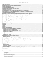
Table Of Contents
Table Of Contents ............................................................................................................................... 1
Introduction to the ProjectCodeMeter software ................................................................................... 4
System Requirements ......................................................................................................................... 5
Quick Getting Started Guide ............................................................................................................... 6
Programming Languages and File Types ............................................................................................ 7
Changing License Key ........................................................................................................................ 9
Steps for Sizing Future Project for Cost Prediction or Price Quote ................................................... 10
Differential Sizing of the Changes Between 2 Revisions of the Same Project .................................. 11
Cumulative Differential Analysis ........................................................................................................ 12
Estimating a Future project schedule and cost for internal budget planning ..................................... 13
Measuring past project for evaluating development team productivity .............................................. 14
Estimating a Future project schedule and cost for producing a price quote ...................................... 15
Monitoring an Ongoing project development team productivity ......................................................... 16
Estimating the Maintainability of a Software Project ......................................................................... 17
Evaluating the attractiveness of an outsourcing price quote ............................................................. 18
Measuring an Existing project cost for producing a price quote ........................................................ 19
Steps for Sizing an Existing Project .................................................................................................. 20
Analysis Results Charts .................................................................................................................... 21
Project Files List ................................................................................................................................ 22
Project selection settings .................................................................................................................. 23
Settings ............................................................................................................................................. 24
Summary .......................................................................................................................................... 28
Toolbar .............................................................................................................................................. 29
Reports ............................................................................................................................................. 30
Report Template Macros ................................................................................................................... 32
Command line parameters and IDE integration ................................................................................ 34
Integration with Microsoft Visual Studio 6 ....................................................................................................................... 34
Integration with Microsoft Visual Studio 2003 - 2010 ...................................................................................................... 35
Integration with CodeBlocks ............................................................................................................................................ 35
Integration with Eclipse ................................................................................................................................................... 36
Integration with Aptana Studio ........................................................................................................................................ 36
Integration with Oracle JDeveloper ................................................................................................................................. 36
Integration with JBuilder .................................................................................................................................................. 37
Weighted Micro Function Points (WMFP) ......................................................................................... 38
Measured Elements ........................................................................................................................................................ 38
Calculation ....................................................................................................................................................................... 38
Average Programmer Profile Weights (APPW) ................................................................................. 40
Compatibility with Software Development Lifecycle (SDLC) methodologies .................................... 41
Development Productivity Monitoring Guidelines and Tips ............................................................... 42
Code Quality Metrics ......................................................................................................................... 43
Code Quality Notes ........................................................................................................................... 44
Quantitative Metrics .......................................................................................................................... 45
COCOMO ......................................................................................................................................... 46
Basic COCOMO .............................................................................................................................................................. 46
Intermediate COCOMO ................................................................................................................................................... 46
Detailed COCOMO .......................................................................................................................................................... 47
Differences Between COCOMO, COSYSMO, REVIC, Function Points and WMFP ......................... 48
Cost model optimal use case comparison table: ............................................................................... 48
COSYSMO ........................................................................................................................................ 49
......................................................................................................................................................... 49
Cyclomatic complexity ...................................................................................................................... 50
Description ...................................................................................................................................................................... 50
Formal definition ........................................................................................................................................................................................................ 51
Etymology / Naming .................................................................................................................................................................................................. 52
Applications ..................................................................................................................................................................... 52
Limiting complexity during development ................................................................................................................................................................... 52
Implications for Software Testing ............................................................................................................................................................................... 52
Cohesion ................................................................................................................................................................................................................... 53
Correlation to number of defects ............................................................................................................................................................................... 53
Process fallout .................................................................................................................................. 54
Halstead complexity measures ......................................................................................................... 55
Calculation ....................................................................................................................................................................... 55
Maintainability Index (MI) .................................................................................................................. 56
Calculation ....................................................................................................................................................................... 56
Process capability index .................................................................................................................... 57
Recommended values .................................................................................................................................................... 57
Relationship to measures of process fallout ................................................................................................................... 58
Example ........................................................................................................................................................................... 58
OpenSource code repositories .......................................................................................................... 60
REVIC ............................................................................................................................................... 61
Six Sigma .......................................................................................................................................... 62
Historical overview .......................................................................................................................................................... 62
Methods ........................................................................................................................................................................... 62
DMAIC ....................................................................................................................................................................................................................... 63
DMADV ..................................................................................................................................................................................................................... 63
Quality management tools and methods used in Six Sigma ..................................................................................................................................... 63
Implementation roles ....................................................................................................................................................... 63
Certification ............................................................................................................................................................................................................... 64
Origin and meaning of the term "six sigma process" ...................................................................................................... 64
Role of the 1.5 sigma shift ......................................................................................................................................................................................... 64
Sigma levels .............................................................................................................................................................................................................. 64
Source lines of code ......................................................................................................................... 66
Measurement methods ................................................................................................................................................... 66
Origins ............................................................................................................................................................................. 66
Usage of SLOC measures .............................................................................................................................................. 66
Example ........................................................................................................................................................................... 67
Advantages ..................................................................................................................................................................... 68
Disadvantages ................................................................................................................................................................. 68
Related terms .................................................................................................................................................................. 69
Logical Lines Of Code (LLOC) .......................................................................................................... 70
General Frequently Asked Questions ............................................................................................... 72
........................................................................................................................................................................................ 72
Is productivity measurements bad for programmers? .................................................................................................... 72
Why not use cost estimation methods like COCOMO or COSYSMO? .......................................................................... 72
What's wrong with counting Lines Of Code (SLOC / LLOC)? ........................................................................................ 72
Does WMFP replace traditional models such as COCOMO and COSYSMO? .............................................................. 72
Technical Frequently Asked Questions ............................................................................................. 73
Are my source code files secure? ................................................................................................................................... 73
Where are XLS spreadsheet reports (for Excel)? ........................................................................................................... 73
Why numbers don't add up or off by a decimal point? .................................................................................................... 73
Why are all results 0? ...................................................................................................................................................... 73
........................................................................................................................................................................................ 73
Why are report files or images missing or not updated? ................................................................................................ 73
Why is the History Report not created or updated? ........................................................................................................ 73
Why can't I see the Charts (there is just an empty space)? ............................................................................................ 73
I analyzed an invalid code file, but I got an estimate with no errors, why? ..................................................................... 74
Can I install without internet connection? ....................................................................................................................... 74
Why header (.h) files aren't measured? .......................................................................................................................... 74
Why do results differ from older ProjectCodeMeter version? ......................................................................................... 74
Where can I start the License or Trial? ........................................................................................................................... 74
What programming languages and file types are supported by ProjectCodeMeter? ..................................................... 74
What do i need to run ProjectCodeMeter? ...................................................................................................................... 74
Accuracy of ProjectCodeMeter ......................................................................................................... 75
ProjectCodeMeter
Is a professional software tool for project managers to measure and estimate the Time, Cost, Complexity, Quality and Maintainability
of software projects as well as Development Team Productivity by analyzing their source code. By using a modern software sizing
algorithm called Weighted Micro Function Points (WMFP) a successor to solid ancestor scientific methods as COCOMO,
COSYSMO, Maintainability Index, Cyclomatic Complexity, and Halstead Complexity, It produces more accurate results than
traditional software sizing tools, while being faster and simpler to configure.
Tip: You can click the icon on the bottom right corner of each area of ProjectCodeMeter to get help specific for that area.
General Introduction
Quick Getting Started Guide
Introduction to ProjectCodeMeter
Quick Function Overview
Measuring project cost and development time
Measuring additional cost and time invested in a project revision
Producing a price quote for an Existing project
Monitoring an Ongoing project development team productivity
Evaluating development team past productivity
Estimating a price quote and schedule for a Future project
Evaluating the attractiveness of an outsourcing price quote
Estimating a Future project schedule and cost for internal budget planning
Evaluating the quality of a project source code
Software Screen Interface
Project Folder Selection
Settings
File List
Charts
Summary
Reports
Extended Information
System Requirements
Supported File Types
Command Line Parameters
Frequently Asked Questions
ProjectCodeMeter
Introduction to the ProjectCodeMeter software
ProjectCodeMeter is a professional software tool for project managers to measure and estimate the Time, Cost, Complexity, Quality
and Maintainability of software projects as well as Development Team Productivity by analyzing their source code. By using a modern
software sizing algorithm called Weighted Micro Function Points (WMFP) a successor to solid ancestor scientific methods as
COCOMO, Cyclomatic Complexity, and Halstead Complexity. It gives more accurate results than traditional software sizing tools,
while being faster and simpler to configure. By using ProjectCodeMeter a project manager can get insight into a software source
code development within minutes, saving hours of browsing through the code.
Software Development Cost Estimation
ProjectCodeMeter measures development effort done in applying a project design into code (by an average programmer), including:
coding, debugging, nominal code refactoring and revision, testing, and bug fixing. In essence, the software is aimed at answering the
question "How long would it take for an average programmer to create this software?" which is the key question in putting a price tag
for a software development effort, rather than the development time it took your particular programmer in you particular office
environment, which may not reflect the price a client may get from a less/more efficient competitor, this is where a solid statistical
model comes in, the APPW which derives its data from study of traditional cost models, as well as numerous new study cases
factoring for modern software development methodologies.
Software Development Cost Prediction
ProjectCodeMeter enables predicting the time and cost it will take to develop a software, by using a feature analogous to the project
you wish to create. This analogy based cost estimation model is based on the premise that it requires less expertise and experience
to select a project with similar functionality, than to accurately answer numerous questions rating project attributes (cost drivers), as in
traditional cost estimation models such as COCOMO, and COSYSMO.
In producing a price quote for implementing a future project, the desired cost estimation is the cost of that implementation by an
average programmer, as this is the closest estimation to the price quote your competitors are offering.
Software Development Productivity Evaluation
Evaluating your development team productivity is a major factor in management decision making, influencing many aspects of project
management, including: role assignments, target product price tag, schedule and budget planning, evaluating market
competitiveness, and evaluating the cost-effectiveness of outsourcing. ProjectCodeMeter allows a project manager to closely follow
the project source code progress within minutes, getting an immediate indication if development productivity drops.
ProjectCodeMeter enables actively monitoring the progress of software development, by adding up multiple analysis measurement
results (called milestones). The result is automatically compared to the Project Time Span, and the APPW statistical model of an
average development team, and (if available) the Actual Time, Producing a productivity percentage value for rating your team
performance.
Software Sizing
The time measurement produced by ProjectCodeMeter gives a standard, objective, reproducible, and comparable value for
evaluating software size, even in cases where two software source codes contain the same line count (SLOC), since WMFP takes
source code complexity into account.
Code Quality Inspection
The code metrics produced by ProjectCodeMeter give an indication to some basic and essential source code qualities that affect
maintainability, reuse and peer review. ProjectCodeMeter also shows textual notices if any of these metrics indicate a problem.
Wide Programming Language Support
ProjectCodeMeter supports many programming languages, including C, C++, C#, Java, ObjectiveC, DigitalMars D, Javascript,
JScript, Flash ActionScript, UnrealEngine, and PHP. see a complete list of supported file types.
See the Quick Getting Started Guide for a basic workflow of using ProjectCodeMeter.
ProjectCodeMeter
System Requirements
- Mouse (or other pointing device such as touchpad or touchscreen)
- Windows NT 5 or better (Windows XP / 2000 / 2003 / Vista / 7)
- Adobe Flash ActiveX plugin 9.0 or newer for IE
- Display resolution 1024x768 16bit color or higher
- Internet connection (for license activation only)
- At least 50MB of writable disk storage space
Optionally recommended:
- WinMerge installed (for viewing textual file differences)
- Microsoft Office Excel installed (for editing reports)
ProjectCodeMeter
Quick Getting Started Guide
ProjectCodeMeter can measure and estimate the Development Time, Cost and Complexity of software projects.
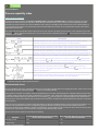
The basic workflow of using ProjectCodeMeter is selecting the Project Folder (1 on the top left), Selecting the appropriate Settings
(2 on the top right) then clicking the Analyze button (3 on the top middle). The results are shown at the bottom, both as Charts (on the
bottom left) and as a Summary (on the bottom right).
For extended result details you can see the File List area (on the middle section) to get per file measurements, as well as look at the
Report files located at the project folder under the newly generated sub-folder ".PCMReports" which can be easily accessed by
clicking the "Reports" button (on the top right).
Tip: You can click the icon on the bottom right corner of each area of ProjectCodeMeter to get help specific for that area.
For detailed step by step instructions see Steps for Sizing an Existing Project.
For more tasks which can be achieved with ProjectCodeMeter see the Function Overview part of the main index.
ProjectCodeMeter
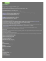
Programming Languages and File Types
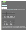
ProjectCodeMeter analyzes the following Programming Languages and File Types:
C expected file extensions .C .CC , [Notes: 1,2,5]
C++ expected file extensions .CPP .CXX , [Notes: 1,2,3,5,7]
C# and SilverLight expected file extensions .CS .ASMX , [Notes: 1,2,5,7]
JavaScript and JScript expected file extensions .JS .JSE .HTML .HTM .ASP .HTA .ASPX , [Notes: 4,5,6]
Objective C expected file extensions .M .MM, [Notes: 5]
UnrealScript v2 and v3 expected file extensions .UC
Flash/Flex ActionScript expected file extensions .AS .MXML
Java expected file extensions .JAVA .JAV .J, [Notes: 5]
J# expected file extensions .JSL, [Notes: 5]
DigitalMars D expected file extensions .D, [Notes: 5]
PHP expected file extensions .PHP, [Notes: 5,6]
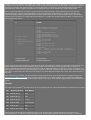
Language Notes and Exceptions:
1. Does not support placing executable code in header files (.h or .hpp)
2. Can not correctly detect using macro definitions for replacing default language syntax, for example: #define LOOP while
3. Accuracy may be reduced with C++ projects extensively using STL operator overloading.
4. Supports semicolon ended statements coding style only.
5. Does not measure inlining a second programming language in the program output, for example embedding JavaScript in PHP:
echo('<script type="text/javascript">window.scrollTo(0,0);</script>');
you will need to include the second language in an external file to be properly measured, for example:
include('scroller.js');
6. Does not measure HTML tags and CSS elements, as these are usually generated by WYSIWYG graphic editors
7. Resource design files ( .RC .RES .RESX .XAML) are not measured
General notes
Your source file name extension should match the programming language inside it (for example naming a PHP code with an .HTML
extension is not supported).
Programming Environments and Runtimes
ProjectCodeMeter supports source code written for almost all environments which use the file types it can analyze. These include:
Oracle/Sun Java Standard Editions (J2SE)
Oracle/Sun Java Enterprise Edition (J2EE)
Oracle/Sun Java Micro Edition (J2ME)
Oracle/Sun Java Developer Kit (JDK)
IBM Java VM and WebSphere
Google Android (SDK, NDK)
WABA JVM (SuperWABA, TotalCross)
Microsoft J# .NET
Microsoft Java Virtual Machine (MS-JVM)
Microsoft C# .NET
Mono
Microsoft SilverLight
Windows Scripting Engine (JScript)
IIS Active Server Pages (ASP)
Nokia QT
Macromedia / Adobe Flash
Adobe Flex
Adobe Flash Builder
Adobe AIR
PHP
SPHP
Apple iPhone iOS
Firefox / Mozilla Gecko Engine
SpiderMonkey engine
Unreal Engine
Gnu GCC (all platforms)
Gnu CGJ (all platforms)
ProjectCodeMeter
Changing License Key
ProjectCodeMeter is bundled with the License Manager application, which was installed in the same folder as ProjectCodeMeter.
If no license exists, Running ProjectCodeMeter will automatically launch the License Manager. To launch it manually go to your
Windows:
Start - Programs - ProjectCodeMeter - LicenseManager.
Alternatively you can run licman.exe from the ProjectCodeMeter installation folder.
To start a trial evaluation of the software, click the "Trial" button on the License Manager.
If you have purchased a License, enter the License Name and Key in the License Manager, then press OK.
Activation of either Trial or a License require an internet connection, after that point you may disconnect from the internet. only
licman.exe connects to the internet licensing server when you select one of the buttons. ProjectCodeMeter.exe does not access the
internet at any point.
NOTES:
In case your internet connection requires a Proxy, Please make sure your proxy settings is set in your windows "Control Panel""Internet Options"-"Connections"-"LAN Settings"
You may need to approve (Unblock) the License Manager (licman.exe) in your Windows Firewall (or ZoneAlarm / Antivirus), or disable
them during activation.
To purchase a license please visit the website: www.ProjectCodeMeter.com
For any licensing questions contact ProjectCodeMeter support at:
email: [email protected]
website: www.ProjectCodeMeter.com/support
ProjectCodeMeter
Steps for Sizing Future Project for Cost Prediction or Price Quote
This process enables predicting the time and cost it will take to develop a software, by using a feature analogous to the project you
wish to create. The closer the functionality of the project you select, the more accurate the results will be. This analogy based cost
estimation model is based on the premise that it requires less expertise and experience to select a project with similar functionality,
than to accurately answer numerous questions rating project attributes (cost drivers), as in traditional cost estimation models such as
COCOMO, and COSYSMO.
In producing a price quote for implementing a future project, the desired cost estimation is the cost of that implementation by an
average programmer, as this is the closest estimation to the price quote your competitors are offering.
Step by step instructions:
1. Select a software project with similar functionality to the future project you plan on developing. Usually an older project of yours, or a
downloaded Open Source project from one of the open source repository websites such as SourceForge (www.sf.net) or Google
Code (code.google.com)
2. Make sure you don't have any open ProjectCodeMeter report files in your spreadsheet or browser, as these files will be updated
3. Put the project source code in a folder on your local disk (excluding any auto generated files, for cost prediction exclude files which
functionality is covered by code library you already have)
4. Select this folder into the Project Folder textbox
5. Select the Settings describing the project (make sure not to select "Differential comparison"). Note that for producing a price quote
it is recommended to select the best Debugging Tools type available for that platform, rather than the ones you have, since your
competitor probably uses these and therefore can afford a lower price quote.
6. Click "Analyze", when the process finishes the results will be at the bottom right summary screen
ProjectCodeMeter
Differential Sizing of the Changes Between 2 Revisions of the Same Project
This process enables comparing an older version of the project to a newer one, as results will measure the time and cost of the delta
(change) between the two versions. ProjectCodeMeter performs a truly differential source code comparison since analysis is based
on a parser, free from the "negative SLOC" problem.
Step by step instructions:
1. Make sure you don't have any open ProjectCodeMeter report files in your spreadsheet or browser, as these files will be updated
2. Put on your local disk a folder with the current project revision (excluding any auto generated files, files created by 3rd party, files
taken from previous projects)
3. Select this folder into the Project Folder textbox
4. Click to select the Differential Comparison checkbox to enable checking only revision differences
5. Put on your local disk a folder with an older revision of your project , can be the code starting point (skeleton or code templates) or
any previous version
6. Select this folder into the Old Version Folder textbox
7. Select the Settings describing the current version of the project
8. Click "Analyze", when the analysis process finishes the results will be shown at the bottom right summary screen
ProjectCodeMeter
Cumulative Differential Analysis
This process enables actively or retroactively monitoring the progress of software development, by adding up multiple analysis
measurement results (called milestones). It is done by comparing the previous version of the project to the current one,
accumulating the time and cost delta (difference) between the two versions.
Only when the software is in this mode, each analysis will be added to History Report, and an auto-backup of the source files will be
made into the ".Previous" sub-folder of your project folder.
Using this process allows to more accurately measure software projects developed using Agile lifecycle methodologies.
Step by step instructions:
1. Make sure you don't have any open ProjectCodeMeter report files in your spreadsheet or browser, as these files will be updated
2. Put on your local disk a folder with the current project revision (excluding any auto generated files, files created by 3rd party, files
taken from previous projects) if you already have such folder from former analysis milestone, then use it instead and copy the latest
source files into it.
3. Select this folder into the Project Folder textbox
4. Click the Differential Comparison checkbox to enable checking only revision differences
5. Clear the Old Version Folder textbox, so that the analysis will be made against the auto-backup version, and an auto-backup will be
created after the first milestone
6. Optionally set the "When analysis ends:" option to "Open History Report" as the History Report is the most relevant to us in this
process
7. Select the Settings describing the current version of the project
8. Click "Analyze", when the analysis process finishes the results for this milestone will be shown at the bottom right summary screen,
While results for the overall project history will be written to the History Report file.
9. Optionally, if you know the actual time it took to develop this project revision from the previous version milestone, you can input the
number (in hours) in the Actual Time column at the end of the milestone row in the History Report file, this will allow you the see the
Average Development Efficiency of your development team (indicated in that report) .
ProjectCodeMeter
Estimating a Future project schedule and cost for internal budget planning
When planning a software project, you need to verify that project development is within the time and budget constraints available to
your organization or allocated to the project, as well as making sure adequate profit margin remains, after deducting costs from the
target price tag.
Step by step instructions:
1. Select a software project with similar functionality to the future project you plan on developing. Usually an older project of yours, or a
downloaded Open Source project from one of the open source repository websites such as SourceForge (www.sf.net) or Google
Code (code.google.com)
2. Make sure you don't have any open ProjectCodeMeter report files in your spreadsheet or browser, as these files will be updated
3. Put the project source code in a folder on your local disk (excluding any auto generated files, and files which functionality is covered
by code libraries you already have)
4. Select this folder into the Project Folder textbox (make sure NOT to select "Differential comparison").
5. Select the Settings describing the project and the tools available to your development team, as well as the actual average Price
Per Hour paid to your developers.
6. Click the "Analyze" button. When analysis finishes, Time and Cost results will be shown at the bottom right summary screen
It is always recommended to plan the budget and time according to average programmer time (as measured by ProjectCodeMeter)
without modification, since even for faster development teams productivity may vary due to personal and environmental
circumstances, and development team personnel may change during the project development lifecycle.
In case you still want to factor for your development team speed, and your development team programmers are faster or slower than
the average (measured previously using Productivity Sizing), divide the resulting time and cost by the factor of this difference, for
example if your development team is twice as fast than an average programming team, divide the time and cost by 2. If your team is
half the speed of the average, then divide the results by 0.5 to get the actual time and cost of development for your particular team.
However, beware not to overestimate the speed of your development team, as it will lead to budget and time overflow.
Use the Project Time and Cost results as the Development component of budget, add the current market average costs for the other
relevant components shown in the diagram above (or if risking factoring for your specific organization, use your organizations average
costs). The resulting price should be the estimated budget and time for the project.
Optionally, You can add the minimal profit percentage making the sale worthwhile, to obtain the bottom margin for a price quote you
produce to your clients. For calculating the top margin for a price quote, use the process Estimating a Future project schedule and
cost for producing a price quote.
ProjectCodeMeter
Measuring past project for evaluating development team productivity
Evaluating your development team productivity is a major factor in management decision making, influencing many aspects of project
management, including: role assignments, target product price tag, schedule planning, evaluating market competitiveness,
compliance with Six Sigma / CMMI / ISO / IEEE / CIPS / SCRUM / LEAN certification, and evaluating the cost-effectiveness of
outsourcing.
This process is suitable for measuring productivity of both single programmers and development teams.
Step by step instructions:
1. Make sure you don't have any open ProjectCodeMeter report files in your spreadsheet or browser, as these files will be updated
2. Using Windows explorer, Identify files to be estimated, usually only files created for this project (excluding files auto-generated by
the development tools, data files, and files provided by a third party)
3. Copy these files to a separate new folder
4. Select this folder into the Project Folder textbox
5. Set the "When analysis ends:" option to "Open Productivity Report" as the Productivity Report is the most relevant in this process
6. Select the Settings describing the project (make sure NOT to select "Differential comparison")
7. Click the "Analyze" button. When analysis finishes, Time results will be shown at the bottom right summary screen
As the Productivity Report will open in your spreadsheet, Fill in the "Assigned personnel" and the "Actual Development Time" fields,
the report will immediately update to show your development team productivity at the bottom line. If your team productivity is below
%100, your development process is less efficient than the average (see tips on How To Improve Developer Productivity).
ProjectCodeMeter
Estimating a Future project schedule and cost for producing a price quote
Whether being a part of a software company or an individual freelancer, when accepting a development contract from a client, you
need to produce a price tag that would beat the price quote given by your competitors, while remaining above the margin of
development costs. The desired cost estimation is the cost of that implementation by an average programmer, as this is the closest
estimation to the price quote your competitors are offering.
Step by step instructions:
1. Select a software project with similar functionality to the future project you plan on developing. Usually an older project of yours, or a
downloaded Open Source project from one of the open source repository websites such as SourceForge (www.sf.net) or Google
Code (code.google.com)
2. Make sure you don't have any open ProjectCodeMeter report files in your spreadsheet or browser, as these files will be updated
3. Put the project source code in a folder on your local disk (excluding any auto-generated files, and files which functionality is covered
by code libraries you already have)
4. Select this folder into the Project Folder textbox (make sure NOT to select "Differential comparison")
5. Select the Settings describing the project. Select the best Debugging Tools settings available for the platform (usually "Complete
system emulator") since your competitors are using these which cuts their development effort thus affording a lower price quote.
Select the Quality Guarantee and Platform Maturity for your future project. The Price Per Hour should be the market average hourly
rate of a programmer with skills for that kind of task.
6. Click the "Analyze" button. When analysis finishes, Time and Cost results will be shown at the bottom right summary screen
Use the Project Time and Cost results as the Development component of the price quote, add the market average costs of the other
relevant components shown in the diagram above. Add the nominal profit percentage suitable for the target market. The resulting price
should be the top margin for the price quote you produce to your clients. For calculating the bottom margin for the price quote, use the
process Estimating a Future project schedule and cost for internal budget planning.
ProjectCodeMeter
Monitoring an Ongoing project development team productivity
This process enables actively monitoring the progress of software development, by adding up multiple analysis measurement results
(called milestones). It is done by comparing the previous version of the project to the current one, accumulating the time and cost delta
(difference) between the two versions.
Only when the software is in this mode, each analysis will be added to the History Report, and an auto-backup of the source files will
be saved into the ".Previous" sub-folder of your project folder.
The process is a variant of Cumulative Differential Analysis which allows to more accurately measure software projects, including
those developed using Agile lifecycle methodologies.
It is suitable for measuring productivity of both single programmers and development teams.
Step by step instructions:
1. Make sure you don't have any open ProjectCodeMeter report files in your spreadsheet or browser, as these files will be updated. If
you want to start a new history tracking, simply rename or delete the old History Report file.
2. Put on your local disk a folder with the most current project source version (excluding any auto generated files, files created by 3rd
party, files taken from previous projects) if you already have such folder from former analysis milestone, then use it instead and copy
the latest version of the source files into it.
3. Select this folder into the Project Folder textbox
4. Click the Differential Comparison checkbox to enable checking only revision differences
5. Clear the Old Version Folder textbox, so that the analysis will be made against the auto-backup version, and an auto-backup will be
created after the first milestone (ProjectCodeMeter will automatically fill in this textbox later with the auto-backup folder)
6. Optionally, set the "When analysis ends:" option to "Open Differential History Report" as the History Report is the most relevant in
this process
7. Select the Settings describing the current version of the project (you should usually ask your developer for the Quality Guarantee
setting, and).
8. Click "Analyze", when the analysis process finishes the results for this milestone will be shown at the bottom right summary screen,
While results for the overall project history will be written to the History Report file, which should now open automatically.
9. On the first analysis, Change the date of the first milestone in the table (the one with all 0 values) to the date the development
started, so that Project Span will be correctly measured (in the History Report file).
10. If the source code analyzed is a skeleton taken from previous projects or a third party, and should not be included in the effort
history, simply delete the current milestone row (last row on the table).
11. Fill in the number of developers who worked simultaneously on this milestone. For example, if the previous milestone was checked
last week and was made by 1 developer, and at the beginning of this week you hired another developer, and both of them worked at
developing the source code for the this weeks milestone, then enter 2 in this milestones "Developers" column (the previous milestone
will still have 1 in its "Developers" column)
12. Optionally, if you know the actual time it took to develop this project revision from the previous version milestone, you can input the
number (in hours) in the Actual Time column at the end of the milestone row, this will allow you to see the Average Actual Productivity of
your development team (indicated in that report) which can give you a more accurate and customizable productivity rating
than Average Span Productivity.
The best practice is to analyze the projects source code weekly.
Each milestone has its own Span Productivity (and if available, also Actual Productivity), these show how well your development team
performs comparing to the APPW statistical model of an average development team. As your team is probably faster or slower than
average, it is recommended you gather at least 4 weekly milestones before deriving any conclusions. For monitoring and detecting
productivity drops (or increases), look at the Span Prod. Delta (and if available, also Actual Prod. Delta) to see changes (delta) in
productivity for this milestone. A positive value means increase in productivity, while negative values indicate a drop. It is
recommended to look into the reasons behind significant increases (above 5) or drops (below -5), which development productivity
improvement steps to take.
Look at the Average Span Productivity (or if available the Average Actual Productivity) percentage of the History Report to see how
well your development team performs comparing to the APPW statistical model of an average development team. A value of 100
indicated that the development team productivity is exactly as expected (according to the source code produced during the project
duration), As higher values indicate higher productivity than average. In case the value drops significantly and steadily below 100, the
development process is less efficient than the average, so it is recommended to see Productivity improvement tips.
ProjectCodeMeter
Estimating the Maintainability of a Software Project
The difficulty in maintaining a software project is a direct result of its overall size (effort and development time), code style and
qualities.
Step by step instructions:
1. Using Windows explorer, Identify files to be evaluated, usually only files created for this project (excluding files auto-generated by
the development tools, data files, and files maintained by a third party)
2. Copy these files to a separate new folder
3. Select this folder into Project Folder
4. Select the Settings describing the project
5. Optionally set the "When analysis ends" action to "Open Quality report" as this report is the most relevant for this task
6. Click "Analyze"
When analysis finishes, the total time (Programming Hours) as well as Code Quality Notes Count will be at the bottom right summary
screen.
The individual quality notes will be at the rightmost column of each file in the file list.
The Quality Report file contains that information as well.
As expected, the bigger the project in Programing Time and the more Quality Notes it has, the harder it will be to maintain.
ProjectCodeMeter
Evaluating the attractiveness of an outsourcing price quote
In order to calculate how cost-effective is a price quote received from an external outsourcing contractor, Price boundaries need to be
calculated:
Top Margin - by using the method for Estimating a price quote and schedule for a Future project
Outsource Margin - by using the method for Estimating a Future project schedule and cost for internal budget planning
Use the Top Margin to determine the maximum price you should pay, if the price quote is higher it is wise to consider a price quote
from another contractor, or develop in-house.
Use the Outsource Margin to determine the price where outsourcing is more cost-effective than developing in-house, though obviously
cost is not the only merit to be considered when developing in-house.
ProjectCodeMeter
Measuring an Existing project cost for producing a price quote
When selling an existing source code, you need to produce a price tag for it that would match the price quote given by your
competitors, while remaining above the margin of development costs.
Step by step instructions:
1. Make sure you don't have any open ProjectCodeMeter report files in your spreadsheet or browser, as these files will be updated
2. Using Windows explorer, Identify files to be estimated, usually only files created for this project (excluding files auto-generated by
the development tools, data files, and files provided by a third party)
3. Copy these files to a separate new folder
4. Select this folder into the Project Folder textbox
5. Select the Settings describing the project (make sure not to select "Differential comparison"), and the real Price Per Hour paid to
you development team.
6. Click the "Analyze" button. When analysis finishes, Time and Cost results will be shown at the bottom right summary screen
Use the Project Time and Cost results as the Development component of the price quote, add the market average costs of the other
relevant components shown in the diagram above. Add the minimal profit percentage suitable for the target market. The resulting price
should be the top margin for the price quote you produce to your clients (to be competitive). For calculating the bottom margin for the
price quote, use the actual cost, plus the minimal profit percentage making the sale worthwhile (to stay profitable). In case the bottom
margin is higher than the top margin, your development process is less efficient than the average, so it is recommended to reassign
personnel to other roles, change development methodology, or gain experience and training for your team.
ProjectCodeMeter
Steps for Sizing an Existing Project
This process enables measuring programming cost and time invested in an existing software project according to the
WMFP algorithm. This process is useful in assessing the effort (work hours) of a single developer or a development team (either inhouse or outsourced). Note that development processes exhibiting high amount of design change require accumulating differential
analysis results, Refer to compatibility notes for using Agile development processes with the the APPW statistical model. For
measuring only the difference from the last version use the Differential Project Sizing process.
Step by step instructions:
1. Make sure you don't have any open ProjectCodeMeter report files in your spreadsheet or browser, as these files will be updated
2. Using Windows explorer, Identify files to be estimated, usually only files created for this project (excluding files auto-generated by
the development tools, data files, and files provided by a third party)
3. Copy these files to a separate new folder
4. Select this folder into the Project Folder textbox
5. Select the Settings describing the project (make sure not to select "Differential comparison").
6. Click the "Analyze" button. When analysis finishes, Time and Cost results will be shown at the bottom right summary screen
ProjectCodeMeter
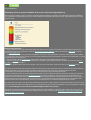
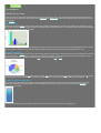
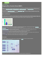
Analysis Results Charts
Charts visualize the data which already exists in the Summary and Report Files. They are only displayed when the analysis process
finishes and valid results for the entire project have been obtained. Stopping the analysis prematurely will prevent showing the charts
and summary.
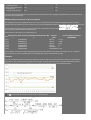
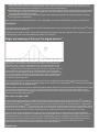
Minute Bar Graph
Shows the measured WMFP metrics for the entire project. Useful for visualizing the amount of time spent by the developer on each
metric type. Result are shown in whole minutes, with optional added single letter suffix: K for thousands, M for Millions. Note that large
numbers are rounded when M or K suffixed.
In the example image above, the Ttl (Total Project Development Time in minutes) indicates 9K, meaning 9000-9999 minutes. The DT
(Data Transfer Development Time) indicates 490, meaning 490 minutes were spent on developing Data Transfer code.
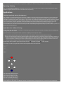
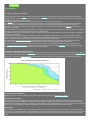
Percentage Pie Chart
Shows the measured WMFP metrics for the entire project. Useful for visualizing the development time and cost distribution according
to each metric type, as well as give an indication to the nature of the project by noticing the dominant metric percentages, as more
mathematically oriented (AI), decision oriented (FC) or data I/O oriented (DT and OV).
In the example image above, the OV (dark blue) is very high, DT (light green) is nominal, FC (orange) is typically low, while AI (yellow)
is not indicated since it is below 1%. This indicates the project nature to be Data oriented, with relatively low complexity.
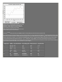
Component Percentage Bar Graph
Shows the development effort percentage for each component relatively to the entire project, as computed by the APPW model.
Useful for visualizing the development time and cost distribution according to the 3 major development components: Coding,
Debugging, and Testing.
In the example image above, the major part of the development time and cost was spent on Coding (61%).
ProjectCodeMeter
Project Files List
Shows a list of all source code files detected as belonging to the project. As analysis progresses, metric details about every file will be
added to the list, each file has its details on the same horizontal row as the file name. Percentage values are given in percents relative
to the file in question (not the whole project). The metrics are given according to the WMFP metric elements, as well as Quality and
Quantitative metrics, and Quality / Maintainability warnings.
Total Time - Shows the calculated programmer time it took to develop that file (including coding, debugging and testing), shown both in
minutes and in hours independently.
Coding - Shows the calculated programmer time spent on coding alone on that file, shown both in minutes and in percentage of total
file development time.
Debugging - Shows the calculated programmer time spent on debugging alone on that file, shown both in minutes and in percentage
of total file development time.
Testing - Shows the calculated programmer time spent on testing alone on that file, shown both in minutes and in percentage of total
file development time.
Flow Complexity, Object Vocabulary, Object Conjuration, Arithmetic, Data Transfer, Code Structure, Inline Data, Comments - Shows
the correlating WMFP source code metric measured for that file, shown both in minutes and in percentage of total file development
time.
CCR, ECF, CSM, LD, SDE, IDF, OCF - Shows the correlating calculated Code Quality Metrics for that file, shown in absolute value.
LLOC, Strings, Numeric Constants - Shows the counted Quantitative Metrics for that file, shown in absolute value.
Quality Notes - Shows warnings on problematic source code qualities and attributes.
Tip: You can right-click a file to do some operations on it, like editing it, open the containing folder and more.
ProjectCodeMeter
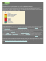
Project selection settings
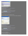
Project folder
Enter the folder (directory) on you local disk where the project source code resides.
1. Clicking it will open the folder in File Explorer
2. Textbox where you can type or paste the folder path
3. Clicking it will open the folder selection dialog that will allow you to browse for the folder, instead of typing it in the textbox.
It is recommended not to use the original folder used for development, rather a copy of the original folder, where you can remove files
that should not be measured:
Auto-generated files - source and data files created by the development environment (IDE) or other automated tools, These are
usually irrelevant since the effort in producing them is very low, yet they have large intrinsic functionality.
Files developed by 3rd party - source and data files taken from a purchased commercial off-the-shelf product, These are usually
irrelevant since the price paid for standard product commercial library is significantly lower.
Files copied from previous projects - Reused source code and library files, These are usually irrelevant since they are either not
delivered to the client in source form, or not sold exclusively to one client, therefore they are priced significantly lower.
Unit Test files - Testing code is mostly auto-generated and trivial, and is already factored for and included in the results. Complex
testing code such as simulators and emulation layers should be treated as a separate project and analyzed separately, using Beta
quality settings.
Differential comparison
Enabling this checkbox will allow you to specify an Old Version Folder, and analyze only the differences between the old version and
the current one (selected in the Project Folder above).
Old Version Folder
Enter the folder (directory) on you local disk where an older version of the source code resides. This allows you to analyze only the
differences between the old version and the current one (selected in the Project Folder above).
This folder often used to designate:
Source code starting point (skeleton or code template) - this will exclude the effort of creating the code starting point, which is often
auto-generated or copied.
Source files of any previous version of the project - Useful in order to get the delta (change) effort from the previous version to the
current.
The auto-backup previous version of the project - You can leave this box empty in order to analyze differences between the autobackup version and the current one, a practice useful for Differential Cumulative Analysis.
When analysis ends
You can select the action that will be taken when the source code analysis finishes. This allows you to automatically open one of the
generated analysis reports, every time the analysis process is finished. To make ProjectCodeMeter automatically exit, select "Exit
application" (useful for batch operation). To prevent this behavior simply select the first option from the list "Just show summary and
charts". Note that all reports are generated and saved, regardless of this setting. You can always browse the folder containing the
generated reports by clicking the "Reports" button, where you can open any of the reports or delete them.
ProjectCodeMeter
Settings
Price per Hour
This value should correlate with the task you are using ProjectCodeMeter for, in most cases you'll want to enter the average hourly rate
of a programmer with skills for this type of project when you use ProjectCodeMeter to calculate the expected cost it takes for an
average programmer to create this project. Likewise, enter the cost of your programmer to estimate the cost it should take your team to
create this project. For specific tasks see the Quick Function Overview section of the main page. If your developers have several pay
grades, Then enter their average hourly rate when measuring their combined source code.
You can enter a number for the cost along with any formatting you wish for representing currency. As an example, all these are valid
inputs: 200, $50, 70 USD, 4000 Yen.
Quality Guarantee
The product quality guaranteed by the programmers' contract. The amount of quality assurance (QA) testing which was done on the
project determines its failure rate. There is no effective way to determine the amount of testing done, except for the
programmers guarantee. QA can be done in several methods (Unit Testing, UI Automation, Manual Checklist), under several Lifecycle
methodologies where quality levels are marked differently for each.
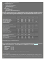
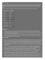
Quality levels stated in Sigma are according to the standard Process Fallout model, as measured in long term Defects Per Million:
1-Sigma 691,462 Defects / Million
2-Sigma 308,538 Defects / Million
3-Sigma 66,807 Defects / Million
4-Sigma 6,210 Defects / Million
5-Sigma 233 Defects / Million
6-Sigma 3.4 Defects / Million
7-Sigma 0.019 Defects / Million
Platform Maturity
The quality of the underlying system platform, measured in average stability and support for all the platform parts, including the Function
library API, Operating System, Hardware, and Development Tools.
You should select "Popular Stable and Documented" for standard architectures like:
Intel and AMD PCs, Windows NT, Sun Java VM, Sun J2ME KVM, Windows Mobile, C runtime library, Apache server, Microsoft IIS,
Popular Linux distros (Ubuntu, RedHat/Fedora, Mandriva, Puppy, DSL), Flash.
Here is a more detailed platform list.
Debugging Tools
The type of debugging tools available to the programmer. Tools are listed in descending efficiency (each tool has the capabilities of all
lower ranked tools). For projects which do not use any external or non-standard hardware or network setup, and a Source Step
Debugger is available, You should select "Complete System Emulator / VM" since in this case the external platform state is irrelevant
thus making a Step Debugger and an Emulator equally useful.
Emulators, Simulators and Virtual Machines (VMs) are top of the line debugging tools, allowing the programmer to simulate the entire
system including the hardware, stop at any given point and examine the internals and status of the system. They are synchronized with
the source step debugger to stop at the same time the debugger does, allowing to step through the source code and the platform
state.
A "Complete System Emulator" allows to pause and examine every hardware component which interacts with the project, while a
"Main Core Emulator" only allows this for the major components (CPU, Display, RAM, Storage, Clock).
Source Step Debuggers allow the programmer to step through each line of the code, pausing and examining internal code variables,
but only very few or no external platform states.
Binary Step Debuggers allow stepping through mchine instuctions (disassembly) and examining data and execution state, but don't
show the original source code.
Debug Text Log is used to write a line of text selected by the programmer to a file, whether directly or through a supporting
hardware/software tool (such as a protocol analyzer or a serial terminal).
Led or Beep Indication is a last resort debugging tool sometimes used by embedded programmers, usually on experimental systems
when supporting tools are not yet available, on reverse engineering unfamiliar hardware, or when advanced tools are too expensive.
ProjectCodeMeter
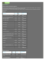
Common software and hardware platforms:
The quality of the underlying system platform, measured in average stability and support for all the platform parts, including the
Function library API, Operating System, Hardware, and Development Tools.
For convenience, here is a list of common platform parts and their ratings, as estimated at the time of publication of this article
(August 2010).
Hardware:
Part Name
Popularity Stability
Documentation
Level
PC Architecture (x86 compatible)
Popular
Stable
Well
documented
CPU x86 compatible (IA32, A64,
MMX, SSE, SSE2)
Popular
Stable
Well
documented
CPU AMD 3DNow
Popular
Stable
Well
documented
CPU ARM core
Stable
Well
documented
Altera FPGA
Stable
Well
documented
Xilinx FPGA
Stable
Well
documented
Atmel AVR
Popular
Stable
Well
documented
MCU Microchip PIC
Popular
Stable
Well
documented
MCU x51 compatible (8051, 8052)
Popular
Stable
Well
documented
MCU Motorola Wireless Modules
(G24)
Stable
Well
documented
MCU Telit Wireless Modules
(GE862/4/5)
Stable
Well
documented
USB bus
Popular
Functional Mostly
documented
PCI bus
Popular
Stable
Mostly
documented
Serial bus (RS232, RS485, TTL)
Popular
Stable
Well
documented
Stable
Mostly
documented
I2C bus
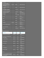
Operating Systems:
Part Name
Popularity Stability
Documentation
Level
Microsoft Windows 2000,
2003, XP, ES, PE, Vista,
Seven
Popular
Stable
Well documented
Functional
Mostly
documented
Microsoft Windows 3.11,
95, 98, 98SE, Millenium,
documented
NT3, NT4
Linux (major distros:
Ubuntu, RedHat/Fedora,
Mandriva, Puppy, DSL,
Slax, Suse)
Stable
Well documented
Linux (distros: Gentoo,
CentOS)
Stable
Well documented
Linux (distros: uCLinux,
PocketLinux, RouterOS)
Functional
Well documented
Windows CE, Handheld,
Smartphone, Mobile,
Functional
Mostly
documented
MacOSX
Stable
Well documented
ReactOS
Experimental Well documented
PSOS
Stable
Mostly
documented
VMX
Stable
Mostly
documented
Solaris
Stable
Well documented
Stable
Mostly
documented
Ericsson Mobile Platform
Stable
Mostly
documented
Apple iPhone IOS
Stable
Mostly
documented
Android
Functional
Well documented
Symbian
Popular
Popular
Function library API:
Part Name
Popularity Stability
Documentation
Level
Oracle/Sun Java SE, EE
Popular
Stable
Well
documented
Oracle/Sun Java ME (CLDC,
CDC, MIDP)
Popular
Stable
Well
documented
C runtime library
Popular
Stable
Well
documented
Apache server
Popular
Stable
Well
documented
Microsoft IIS
Popular
Stable
Well
documented
Flash
Popular
Stable
Mostly
documented
Stable
Mostly
documented
Stable
Well
documented
UnrealEngine
Microsoft .NET
Popular
Functional Well
documented
Mono
Gecko / SpiderMonkey (Mozilla,
Firefox, SeaMonkey, K-Meleon,
Aurora, Midori)
Popular
Stable
Well
documented
Microsoft Internet Explorer
Apple WebKit (Safari)
Popular
Stable
Well
documented
Stable
Well
documented
ProjectCodeMeter
Summary
Shows a textual summary of metric details measured for the entire project. Percentage values are given in percents relative to the
whole project. The metrics are given according to the WMFP metric elements, as well as Quality and Quantitative metrics. In Normal
Analysis, results show the entire project measurement, while in Differential mode, the results measure only the difference from the old
version. For comparison purposes, measured COCOMO and REVIC results are also shown, Please note the Differences Between
COCOMO and WMFP results.
You can compare the Total Time result with the actual time it took your team to develop the project. In case the actual time is higher
than the calculated time results, your development process is less efficient than the average. However, it's easier to use the
Productivity Report to get your developer productivity.
ProjectCodeMeter
Toolbar
The toolbar buttons on the top right of the application, provide the following actions:
Reports
This button allows you to browse the folder containing the generated reports using Windows File Explorer, where you can open any of
the reports or delete them. This button is only available after the analysis has finished, and the reports have been generated.
Save Settings
This allows you to save all the settings of ProjectCodeMeter, which you can load later using the Load Settings button, or the command
line parameters.
Load Settings
This allows loading a previously saved setting.
Help
Brings up this help window, showing the main index. To see context relevant help for a specific screen area, click the icon in the
application screen near that area.
Basic UI / Full UI
This button switches between Basic and Full User Interface. In effect, the Basic UI hides the result area of the screen, until it is needed
(when analysis finishes).
ProjectCodeMeter
Reports
When analysis finishes, several report files are created in the project folder under the newly generated sub-folder ".PCMReports"
which can be easily accessed by clicking the "Reports" button (on the top right). Most reports are available in 2 flavors: HTM and CSV
files.
HTM files are in the same format as web pages (HTML) and can be read by any Internet browser (such as Internet Explorer, Firefox,
Opera), but they can also be read by most spreadsheet applications (such as Microsoft Excel, Gnumeric, LibreOffice Calc) which is
preferable since some reports contain spreadsheet formulas, colors and alignment of the data fields. NOTE: only Microsoft Excel
supports updating HTML report files correctly.
CSV files are in simplified and standard format which can be read by any spreadsheet application (such as Spread32, Office Mobile,
Microsoft Excel, LibreOffice Calc, OpenOffice Calc, Gnumeric) however this file type does not support colors, and some
spreadsheets do not show or save formulas correctly.
Tips:
Printing the HTML report can be done in your spreadsheet application or browser. Firefox has better image quality, but Internet
Explorer shows data aligned and positioned better.
Summary Report
This report summarizes the WMFP, Quality and Quantitative results for the entire project as measured by the last analysis. It is used
for overviewing the project measurement results and is the most frequently used report. This report file is generated and overwritten
every time you complete an analysis. The file names for this report are distinguished by ending with the word "_Summary".
Time Report
This report shows per file result details, as measured by the last analysis. It is used for inspecting detailed time measurements for
several aspects of the source code development. Each file has its details on the same horizontal row as the file name, where
measurement values are given in minutes relevant to the file in question, and the property (metric) relevant to that column. The bottom
line shows the Totals sum for the whole project. This report file is generated and overwritten every time you complete an analysis. The
file names for this report are distinguished by ending with the word "_Time".
Quality Report
This report shows per file Quality result details, as measured by the last analysis. It is used for inspecting some quality properties of
the source code as well as getting warnings and tips for quality improvements (on the last column). Each file has its details on the
same horizontal row as the file name, where measurement values marked with % are given in percents relative to the file in question
(not the whole project), other measurements are given in absolute value for the specific file. The bottom line shows the Totals sum for
the whole project. This report file is generated and overwritten every time you complete an analysis. The file names for this report are
distinguished by ending with the word "_Quality".
Reference Model Report
This report shows calculated traditional Cost Models for the entire project as measured by the last analysis. It is used for reference
and algorithm comparison purposes. Includes values for COCOMO, COCOMO II 2000, and REVIC 9.2. The Nominal and Basic
values are for a typical standard project, while the Intermediate values are influenced by metrics automatically measured for the
project. This report file is generated and overwritten every time you complete an analysis. The file names for this report are
distinguished by ending with the word "_Reference".
Productivity Report
This report is used for calculating your Development Team Productivity comparing to the average statistical data of the APPW model.
You need to open it in a spreadsheet program such as Gnumeric or Microsoft Excel, and enter the Actual Development Time it took
your team to develop this code - the resulting Productivity percentage will automatically be calculated and shown at the bottom of the
report. In case the value drops significantly and steadily below 100, the development process is less efficient than the average, so it is
recommended to see Development productivity improvement tips. This report file is generated and overwritten every time you
complete an analysis. The file names for this report are distinguished by ending with the word "_Productivity".
Differential Analysis History Report
This report shows history of analysis results. It is used for inspecting development progress over multiple analysis cases (milestones)
when using Cumulative Differential Analysis. Each milestone has its own row containing the date it was performed and its analysis
result details. Measurements are given in absolute value for the specific milestone (time is in hours unless otherwise noted). The first
milestone indicates the project starting point, so all its measurement values are set to 0, it is usually required to manually change its
date to the actual projects starting date in order for the Project Span calculations to be effective. It is recommended to analyze a new
sourcecode milestone at every specification or architectural redesign, but not more than once a week as statistical models have
higher deviation with smaller datasets. This report file is created once on the first Cumulative Differential Analysis and is
updated every time you complete a Cumulative Differential Analysis thereafter. The file names for this report are distinguished by
ending with the word "_History".
The summary at the top shows the Totals sum for the whole history of the project:
Work hours per Month (Yearly Average) - Input the net monthly work hours customary in your area or market, adjusted for holidays (152
for USA). This field is editable.
Total Expected Project Hours - The total sum of the development hours for all milestones calculated by ProjectCodeMeter. This
indicates how long the entire project history should take.
Total Expected Project Cost - The total sum of the development cost for all milestones calculated by ProjectCodeMeter. This indicates
how much the entire project history should cost.
Total Modified Logical Lines of Code (LLOC) - The total number of source code lines changed during the entire project history.
Average Cost Per Hour - The calculated average pay per hour across the project milestone history. Useful if the programmers pay has
changed over the course of the project, and you need to get the average hourly rate.
Analysis Milestones - The count of analysis cases (rows) in the bottom table.
Project Span Days - The count of days passed from the first milestone to the last, according to the milestone dates. Useful for seeing
the gross sum of actual days that passed from the projects' beginning.
Project Span Hours - The net work hours passed from the projects beginning, according to the yearly average working hours.
Average Project Span Productivity % - Your development team productivity compared to the statistical average based on the balance
between the WMFP expected development time and the project span, shown in percents. Value of 100 indicated that the development
team productivity is exactly as expected according to the source code produced during project duration, As higher values indicate
higher productivity than average. Note that holidays (and other out of work days) may adversely affect this index in the short term, but
will even out in the long run. Also note that this index is only valid when analyzing each milestone using the most current source code
revision.
Total Actual Development Hours - The total sum of the development hours for all milestones, as was entered for each milestone into
this report by the user (on the Actual Time column). The best practice is to analyze the projects source code weekly, if you do so the
value you need to enter into the Actual Time column is the number of work hours in your organization that week. Note that if you have
not manually updated the Actual Time column for the individual milestones, this will result in a value of 0.
Average Actual Productivity % - Your development team productivity compared to the statistical average based on the balance
between the WMFP expected development time and the Actual Time entered by the user, shown in percents. Value of 100 indicated
that the development team productivity is exactly as expected (according to the source code produced during project duration), As
higher values indicate higher productivity than average. Note that holidays (and other out of work days) may adversely affect this index
in the short term, but will even out in the long run. Also note that this index is only valid if the user manually updated the Actual Time
column for the individual milestones, and when analyzing each milestone using the most current source code revision.
User Templates
You can create any custom report using User Templates. To create a report, create a files of any type and put it in the UserTemplates
folder under the ProjectCodeMeter installation folder (see this folder for examples). When ProjectCodeMeter finishes an analysis, it
will copy your report file to the analyzed project reports folder, and replace any macros inside it with the real values measured for that
analysis, see a list of Report Template Macros. You can use this custom report engine to create any type of reports, in almost any file
type, or even create your own cost model spreadsheet by generating an Excel HTML report that calculates time and cost by taking the
measured code metrics and using them in your own Excel function formula (see the file ProjectCodeMeter_Productivity.xls as an
example)
ProjectCodeMeter
Report Template Macros
You can create any custom report using User Templates. To create a report, create a files of any type and put it in the UserTemplates
folder under the ProjectCodeMeter installation folder. When ProjectCodeMeter finishes an analysis, it will take your report file and
replace any macros inside it with the real values measured for that analysis.
Report Template Macros:
__SOFTWARE_VERSION__ replaced with ProjectCodeMeter version
__LICENSE_USER__ replaced with ProjectCodeMeter licensed user name
__PROJECT_FOLDER__ replaced with the Project Folder
__OLD_FOLDER__ replaced with Old Version Folder
__REPORTS_FOLDER__ replaced with project Reports folder
__ANALYSIS_TYPE__ replaced with analysis type Differential or Normal
__PRICE_PER_HOUR__ replaced with programmer Price Per Hour
__PRICE_PER_HOUR_FORMATTED__ replaced with the currency unit decorated version of the programmer Price Per Hour
__TOTAL_COST_FORMATTED__ replaced with the currency unit decorated version of the total project cost
__COST_UNITS__ replaced with the currency unit decoration if any
__TOTAL_COST__ replaced with the total project cost
__TOTAL_TIME_HOURS__ replaced with the total project time in hours
__TOTAL_TIME_MINUTES__ replaced with the total project time in minutes
__TOTAL_CODING_MINUTES__ replaced with the total project coding time in minutes
__TOTAL_DEBUGGING_MINUTES__ replaced with the total project debugging time in minutes
__TOTAL_TESTING_MINUTES__ replaced with the total project testing time in minutes
__TOTAL_LLOC__ replaced with the project total Logical Source Lines Of Code (LLOC)
__TOTAL_NUMERIC_CONSTANTS__ replaced with the project total Numeric Constants count
__TOTAL_FILES__ replaced with the project total File Count
__TOTAL_STRINGS__ replaced with the project total String Count
__TOTAL_COMMENTS__ replaced with the project total source Comment count
__COCOMO_BASIC_MINUTES__ replaced with the reference Basic COCOMO estimated project time in minutes
__COCOMO_INTERMEDIATE_MINUTES__ replaced with the reference Intermediate COCOMO auto-estimated project time in
minutes
__COCOMO_INTERMEDIATE_RELY__ replaced with the reference Intermediate COCOMO auto-estimated RELY cost driver
__COCOMO_INTERMEDIATE_CPLX__ replaced with the reference Intermediate COCOMO auto-estimated CPLX cost driver
__COCOMO_INTERMEDIATE_TOOL__ replaced with the reference Intermediate COCOMO auto-estimated TOOL cost driver
__COCOMO_INTERMEDIATE_PVOL__ replaced with the reference Intermediate COCOMO auto-estimated PVOL cost driver
__COCOMOII2000_NOMINAL_MINUTES__ replaced with the reference COCOMO II 2000 nominal (normal) estimated project time
in minutes
__COCOMOII2000_INTERMEDIATE_MINUTES__ replaced with the reference Intermediate COCOMO II 2000 auto-estimated
project time in minutes
__COCOMOII2000_INTERMEDIATE_RELY__ replaced with the reference Intermediate COCOMO II 2000 auto-estimated RELY cost
driver
__COCOMOII2000_INTERMEDIATE_CPLX__ replaced with the reference Intermediate COCOMO II 2000 auto-estimated CPLX
cost driver
__COCOMOII2000_INTERMEDIATE_TOOL__ replaced with the reference Intermediate COCOMO II 2000 auto-estimated TOOL
cost driver
__COCOMOII2000_INTERMEDIATE_PVOL__ replaced with the reference Intermediate COCOMO II 2000 auto-estimated PVOL
cost driver
__REVIC92_NOMINAL_EFFORT_MINUTES__ replaced with the reference Nominal Revic 9.2 Effort estimated development time in
minutes
__REVIC92_NOMINAL_REVIEW_MINUTES__ replaced with the reference Nominal Revic 9.2 Review Phase estimated time in
minutes
__REVIC92_NOMINAL_EVALUATION_MINUTES__ replaced with the reference Nominal Revic 9.2 Evaluation Phase
estimated time in minutes
__REVIC92_NOMINAL_TOTAL_MINUTES__ replaced with the reference Nominal Revic 9.2 Total estimated project time in minutes
__REVIC92_EFFORT_MINUTES__ replaced with the reference Revic 9.2 Effort auto-estimated development time in minutes
__REVIC92_REVIEW_MINUTES__ replaced with the reference Revic 9.2 Review Phase auto-estimated time in minutes
__REVIC92_EVALUATION_MINUTES__ replaced with the reference Revic 9.2 Evaluation Phase auto-estimated time in minutes
__REVIC92_TOTAL_MINUTES__ replaced with the reference Revic 9.2 Total auto-estimated project time in minutes
__REVIC92_RELY__ replaced with the reference Revic 9.2 auto-estimated RELY cost driver
__REVIC92_CPLX__ replaced with the reference Revic 9.2 auto-estimated CPLX cost driver
__REVIC92_TOOL__ replaced with the reference Revic 9.2 auto-estimated TOOL cost driver
__TOTAL_QUALITY_NOTES__ replaced with count of quality notes and warnings for all files in the project
__CURRENT_DATE_MMDDYYYY__ replaced with todays date in MM/DD/YYYY format (compatible with Microsoft Excel)
__CURRENT_DATE_YYYYMMDD__ replaced with todays date in YYYY-MM-DD format (compatible alphabet sorted lists)
__CURRENT_TIME_HHMMSS__ replaced with the current time in HH:MM:SS format
__QUALITY_NOTES__ replaced with textual quality notes and warnings for the project (not for individual files)
__QUALITY_NOTES__ replaced with textual quality notes and warnings for the project (not for individual files)
__PLATFORM_MATURITY__ replaced with Platform Maturity settings text
__DEBUGGING_TOOLS__ replaced with Debugging Tools settings text
__QUALITY_GUARANTEE__ replaced with Quality Guarantee settings text
__PLATFORM_MATURITY_VALUE__ replaced with Platform Maturity settings as a number
__DEBUGGING_TOOLS_VALUE__ replaced with Debugging Tools settings as a number
__QUALITY_GUARANTEE_VALUE__ replaced with Quality Guarantee settings as a number
__TOTAL_FC_MINUTES__ replaced with the total project time in minutes spent on Flow Complexity
__TOTAL_OV_MINUTES__ replaced with the total project time in minutes spent on Object Vocabulary
__TOTAL_OC_MINUTES__ replaced with the total project time in minutes spent on Object Conjuration
__TOTAL_AI_MINUTES__ replaced with the total project time in minutes spent on Arithmetic Intricacy
__TOTAL_DT_MINUTES__ replaced with the total project time in minutes spent on Data Transfer
__TOTAL_CS_MINUTES__ replaced with the total project time in minutes spent on Code Structure
__TOTAL_ID_MINUTES__ replaced with the total project time in minutes spent on Inline Data
__TOTAL_CM_MINUTES__ replaced with the total project time in minutes spent on Comments
__TOTAL_FC_PERCENT__ replaced with the percent of total project time spent on Flow Complexity
__TOTAL_OV_PERCENT__ replaced with the percent of total project time spent on Object Vocabulary
__TOTAL_OC_PERCENT__ replaced with the percent of total project time spent on Object Conjuration
__TOTAL_AI_PERCENT__ replaced with the percent of total project time spent on Arithmetic Intricacy
__TOTAL_DT_PERCENT__ replaced with the percent of total project time spent on Data Transfer
__TOTAL_CS_PERCENT__ replaced with the percent of total project time spent on Code Structure
__TOTAL_ID_PERCENT__ replaced with the percent of total project time spent on Inline Data
__TOTAL_CM_PERCENT__ replaced with the percent of total project time spent on Comments
ProjectCodeMeter
Command line parameters and IDE integration
When launched, ProjectCodeMeter can optionally accept several command line parameters for automating some tasks, such as a
weekly scan of project files.
These commands can be used from any one of these places:
- Typed from the command prompt
- In a the "Target" of a shortcut properties
- A batch file (for example filename.bat)
- The Windows Start menu "Run" box
- The execution command of any software which supports external applications (such as the Tools menu of Microsoft Visual Studio).
Parameters
/S:SettingsName
This command will load a setting called SettingsName. You should save a setting with that name before using this command (by using
the Save Settings toolbar button). Note that loading a setting will load all ProjectCodeMeter settings, including the Project Folder, and
the When analysis ends Action.
To make ProjectCodeMeter automatically exit, simply select the "When analysis ends" Action of "Exit application".
/A
This command will automatically start the Analysis process when ProjectCodeMeter launchs. Note that it will use the previous Settings
unless you also use the /S command described above.
/X
This command will make ProjectCodeMeter automatically exit when the analysis process finishs. Note that this is independent of any
"When analysis ends" action loaded by the /S command described above (so you can use a settings that opens a report in Excel, and
still exits when finished).
/P:"folder"
This command will set the current Project folder. Use a fully qualified path to the folder of the project you wish to analyze. Can optionally
use single quotes /P:'folder' in case of trouble.
/D
This command will enable Differential comparison mode of analysis
/D:"folder"
This command will enable Differential comparison mode of analysis, and set the Old Version folder
Examples
The following examples assume you installed ProjectCodeMeter into C:\Program Files\ProjectCodeMeter , if that's not the case,
simply use the path you installed to instead.
A typical execution command can look like this:
"C:\Program Files\ProjectCodeMeter\ProjectCodeMeter.exe" /S:MyFirstProjectSetting /P:"C:\MyProjects\MyApp" /A
This will load a setting called MyFirstProjectSetting, set the Project folder to C:\MyProjects\MyApp , and then start the analysis.
Another example may be:
"C:\Program Files\ProjectCodeMeter\ProjectCodeMeter.exe" /P:"C:\MyProjects\MyApp" /D:"C:\MyProjects\MyAppPrevious" /A
This will start a differential analysis between the project version in C:\MyProjects\MyApp and the older version in
C:\MyProjects\MyAppPrevious
Integration with Microsoft Visual Studio 6
Under the Tools - Customize... menu:
Manual analysis of the entire project:
Title: ProjectCodeMeter
Command: C:\Program Files\ProjectCodeMeter\ProjectCodeMeter.exe
Arguments: /P:"$(WkspDir)"
Initial Directory: C:\Program Files\ProjectCodeMeter
all optional checkboxes should be unchecked.
Automatic cumulative analysis milestone (differential from the last analysis):
Title: ProjectCodeMeter Cumulative Milestone
Command: C:\Program Files\ProjectCodeMeter\ProjectCodeMeter.exe
Arguments: /P:"$(WkspDir)" /D /A
Initial Directory: C:\Program Files\ProjectCodeMeter
all optional checkboxes should be unchecked.
Integration with Microsoft Visual Studio 2003 - 2010
Under the Tools - External Tools.. menu (you may need to first click Tools - Settings - Expert Settings):
Manual analysis of the entire project:
Title: ProjectCodeMeter
Command: C:\Program Files\ProjectCodeMeter\ProjectCodeMeter.exe
Arguments: /P:'$(SolutionDir)'
Initial Directory: C:\Program Files\ProjectCodeMeter
all optional checkboxes should be unchecked.
Automatic cumulative analysis milestone (differential from the last analysis):
Title: ProjectCodeMeter Cumulative Milestone
Command: C:\Program Files\ProjectCodeMeter\ProjectCodeMeter.exe
Arguments: /P:'$(SolutionDir)' /D /A
Initial Directory: C:\Program Files\ProjectCodeMeter
all optional checkboxes should be unchecked.
Integration with CodeBlocks
Under the Tools - Configure Tools.. - Add menu:
Manual analysis of the entire project:
Name: ProjectCodeMeter
Executable: C:\Program Files\ProjectCodeMeter\ProjectCodeMeter.exe
Parameters: /P:'${PROJECT_DIR}'
Working Directory: C:\Program Files\ProjectCodeMeter
Select Launch tool visible detached (without output redirection)
Automatic cumulative analysis milestone (differential from the last analysis):
Name: ProjectCodeMeter Cumulative Milestone
Executable: C:\Program Files\ProjectCodeMeter\ProjectCodeMeter.exe
Parameters: /P:'${PROJECT_DIR}' /D /A
Working Directory: C:\Program Files\ProjectCodeMeter
Select Launch tool visible detached (without output redirection)
Integration with Eclipse
Under the Run - External Tools.. - External Tools... - Program - New - Main menu:
Manual analysis of the entire project:
Name: ProjectCodeMeter
Location: C:\Program Files\ProjectCodeMeter\ProjectCodeMeter.exe
Arguments: /P:'${workspace_loc}'
Working Directory: C:\Program Files\ProjectCodeMeter
Display in Favorites: Yes
Automatic cumulative analysis milestone (differential from the last analysis):
Name: ProjectCodeMeter Cumulative Milestone
Location: C:\Program Files\ProjectCodeMeter\ProjectCodeMeter.exe
Arguments: /P:'${workspace_loc}' /D /A
Working Directory: C:\Program Files\ProjectCodeMeter
Display in Favorites: Yes
Integration with Aptana Studio
Under the Run - External Tools - External Tools Configurations... - Program - New - Main menu:
Manual analysis of the entire project:
Name: ProjectCodeMeter
Location: C:\Program Files\ProjectCodeMeter\ProjectCodeMeter.exe
Arguments: /P:'${workspace_loc}'
Working Directory: C:\Program Files\ProjectCodeMeter
Display in Favorites: Yes
Automatic cumulative analysis milestone (differential from the last analysis):
Name: ProjectCodeMeter Cumulative Milestone
Location: C:\Program Files\ProjectCodeMeter\ProjectCodeMeter.exe
Arguments: /P:'${workspace_loc}' /D /A
Working Directory: C:\Program Files\ProjectCodeMeter
Display in Favorites: Yes
Integration with Oracle JDeveloper
Under the Tools - External Tools.. - New - External Program - menu:
Manual analysis of the entire project:
Program Executable: C:\Program Files\ProjectCodeMeter\ProjectCodeMeter.exe
Arguments: /P:'${project.dir}'
Run Directory: "C:\Program Files\ProjectCodeMeter"
Caption: ProjectCodeMeter
Automatic cumulative analysis milestone (differential from the last analysis):
Program Executable: C:\Program Files\ProjectCodeMeter\ProjectCodeMeter.exe
Arguments: /P:'${project.dir}' /D /A
Run Directory: C:\Program Files\ProjectCodeMeter
Caption: ProjectCodeMeter Cumulative Milestone
Integration with JBuilder
Under the Tools - Configure Tools.. - Add menu:
Manual analysis of the entire project:
Title: ProjectCodeMeter
Program: C:\Program Files\ProjectCodeMeter\ProjectCodeMeter.exe
Parameters: /P:'($ProjectDir)'
Unselect Service checkbox, select the Save all checkbox
Automatic cumulative analysis milestone (differential from the last analysis):
Title: ProjectCodeMeter Cumulative Milestone
Program: C:\Program Files\ProjectCodeMeter\ProjectCodeMeter.exe
Parameters: /P:'($ProjectDir)' /D /A
Unselect Service checkbox, select the Save all checkbox
ProjectCodeMeter
Weighted Micro Function Points (WMFP)
WMFP is a modern software sizing algorithm invented by Logical Solutions in 2009 which is a successor to solid ancestor scientific
methods as COCOMO, COSYSMO, Maintainability Index, Cyclomatic Complexity, and Halstead Complexity, It produces more
accurate results than traditional software sizing tools, while requiring less configuration and knowledge from the end user, as most of
the estimation is based on automatic measurements of an existing source code.
As many ancestor measurement methods use source Lines Of Code (LOC) to measure software size, WMFP uses a parser to
understand the source code breaking it down into micro functions and derive several code complexity and volume metrics, which
are then dynamically interpolated into a final effort score.
Measured Elements
The WMFP measured elements are several different metrics deduced from the source code by the WMFP algorithm analysis. They
are represented as percentage of the whole unit (project or file) effort, and are translated into time. ProjectCodeMeter displays these
elements both in units of absolute minutes and in percentage of the file or project, according to the context.
Flow Complexity (FC) - Measures the complexity of a programs' flow control path in a similar way to the traditional Cyclomatic
Complexity, with higher accuracy by using weights and relations calculation.
Object Vocabulary (OV) - Measures the quantity of unique information contained by the programs' source code, similar to the traditional
Halstead Vocabulary with dynamic language compensation.
Object Conjuration (OC) - Measures the quantity of usage done by information contained by the programs' source code.
Arithmetic Intricacy (AI) - Measures the complexity of arithmetic calculations across the program
Data Transfer (DT) - Measures the manipulation of data structures inside the program
Code Structure (CS) - Measures the amount of effort spent on the program structure such as separating code into classes and
functions
Inline Data (ID) - Measures the amount of effort spent on the embedding hard coded data
Comments (CM) - Measures the amount of effort spent on writing program comments
Calculation
The WMFP algorithm uses a 3 stage process: Function Analysis, APPW Transform, and Result Translation.
as shown in the following diagram:
A dynamic algorithm balances and sums the measured elements and produces a total effort score.
M = the Source Metrics value measured by the WMFP analysis stage
W = the adjusted Weight assigned to metric M by the APPW model
N = the count of metric types
i = the current metric type index (iteration)
D = the cost drivers factor supplied by the user input
q = the current cost driver index (iteration)
K = the count of cost drivers
This score is then transformed into time by applying a statistical model called Average Programmer Profile Weights (APPW) which is
a proprietary successor to COCOMO II 2000 and COSYSMO. The resulting time in Programmer Work Hours is then multiplied by a
user defined Cost Per Hour of an average programmer, to produce an average project cost, translated to the user currency.
See also Differences Between COCOMO, COSYSMO, REVIC, Function Points and WMFP
ProjectCodeMeter
Average Programmer Profile Weights (APPW)
APPW is a modern Software Engineering Statistical Cost Model created by Logical Solutions in 2009 team of software experts
experienced with traditional cost models COCOMO, COSYSMO , FISMA, COSMIC, KISS, and NESMA, which knowledge base
constitues 5662 industrial and military projects. The team has coducted a 12 month research adding further statistical study cases of
additional 48 software projects of diverse sizes, platforms and developers, focusing on commercial and open-source projects. Tightly
integrated with the WMFP source code sizing algorithm, allowed to produce a semi-automatic cost model requireing fewer input cost
drivers by completing the necessay information from the measured metrics provided by the WMFP analysis.
APPW model is highly suited for evalutaion of commercial software projects, Therefore the model assumes several precoditions
essential for commercial project development:
A. The programmers are experienced with the language, platform, development methodologies and tools required for the project.
B. Project design and specifications document had been written, or a functional design stage will be separatly measured.
The APPW satistical model has been calibrated to be compatible with the most Sotware Development Lifecycle (SDLC)
methodologies. See SDLC Compatibility notes.
Note that the model measures only development time, It does not measure peripheral effort on learning, researching,
designing, documenting, packaging and marketing.
ProjectCodeMeter
Compatibility with Software Development Lifecycle (SDLC) methodologies
The APPW statistical model has been calibrated to be compatible with the following Software Development Lifecycle (SDLC)
methodologies:
Motorola Six Sigma - Matching the calibrated target quality levels noted on the settings interface, where the number of DMADV cycles
match the sigma level.
Total Quality Managment (TQM) - Matching the calibrated target quality levels noted on the settings interface.
Boehm Spiral - Where project milestones Prototype1, Prototype2, Operational Prototype, Release correspond to the Alpha, Beta,
Pre-Release, Release quality settings.
Kaizen - Requires accumulating differential analysis measurments at every redesign cycle if PDCA cycle count exceeds 3 or design
delta per cycle exceeds 4%.
Agile (AUP/Lean/XP/DSDM) - Requires accumulating differential analysis measurments at every redesign cycle (iteration).
Waterfall (BDUF) - Assuming nominal 1-9% design flaw.
Iterative and incremental development - Requires accumulating differential analysis measurments at every redesign cycle (iteration).
Test Driven Development (TDD) - Requires accumulating differential analysis measurments if overall redesign exceeds %6.
ProjectCodeMeter
Development Productivity Monitoring Guidelines and Tips
ProjectCodeMeter enables actively monitoring the progress of software development, by using the Productivity Monitoring process. In
case the productivity drops significantly and steadily, it is recommended to improve the accuracy of the project design specifications,
improve work environment, purchase development support tools, reassign personnel to other roles, change development
methodology, outsource project tasks which your team has difficulty with, gain experience and training for your team by enrolling them
to complementary seminars or hiring an external consultant.
Studies done by IBM showed the most crucial factor in software development productivity is work environment conditions, as
development teams in private, quiet, comfortable, uninterrupted environments were 260% more productive.
The second most important factor is team interactions and interdependency. Wisely splitting the project development tasks into small
self-contained units, then splitting your team into small groups based on these tasks, will reduce the amount of interactions and
interdependency, exponentially increasing team productivity.
In early design stage, creating a simple as possible control flow, elegant and intuitive code structure, and using clear and accurate
function descriptions, can significantly reduce development time .
Using source code comments extensively can dramatically reduce development time on projects larger than 1 man month, increase
code reuse, and shorten programmer adjustment during personnel reassignment.
Performance review is best done weekly, in order to have enough data points to see an average performance baseline. The purpose
of which is for the manager to detect drops and issues in team performance and fix them, not as a scare tactics to keep developers
"in line" so to speak, it should be done without involving the developers in the process, as developers may be distracted or stressed
by the review itself, or the implications of it, as shown by the Karl Duncker candle experiment, that too high motivational drive may
damage creativity.
ProjectCodeMeter
Code Quality Metrics
These code metrics give an indication to some basic source code qualities that affect maintainability, reuse and peer review.
ProjectCodeMeter also shows textual notices in the Quality Notes section of the Summary and the Quality Report if any of these
metrics indicate a problem.
Code Quality Notes Count - Shows the number of warnings indicating quality issues. Ideally this should be 0, higher values indicate the
code will be difficult to maintain.
Code to Comment Ratio (CCR) - Shows balance between Comment lines and Code Statements (LLOC), A value of 100 means
there's a comment for every code line, lower means only some of the code lines have comments, while higher means that there is
more than one comment for each code line. For example a value of 60 means that only 60% of the code statements have comments.
notice that this is an average, so comments may not be dispersed evenly across the file.
Essential Comment Factor (ECF) - Shows balance between High Quality Comment lines and important Code Statements (Code
Line). An important code statement is a statement which has a higher degree of complexity. A value of 100 means there's a high
quality comment for every important code statement, lower means only some of the code lines have comments, while higher means
that there is more than one comment for each code line. For example a value of 60 means that only 60% of the important code
statements have high quality comments. This indication is important as it is essential that complex lines of code have comments
explaining them. Notice that this is an average, so comments may not be dispersed evenly across the file.
Code Structure Modularity (CSM) - Indicates the degree to which the code is divided into classes and functions. Values around 100
indicate a good balance of code per module, lower values indicate low modularity (bulky code), and higher values indicate fragmented
code.
Logic Density (LD) - Indicates how condensed the logic within the program code. Lower values mean less logic is packed into the
code thus may indicate straight-forward or auto-generated code, while higher values indicate code that is more likely to be generated
by a person.
Source Divergence Entropy (SDE) - Indicates the degree to which objects are manipulated by logic. higher value mean more
manipulation.
Information Diversity Factor (IDF) - Indicates how much reuse is done with objects. higher value mean more reuse.
Object Convolution Factor (OCF) - Shows the degree to which objects interact with each other. higher value means more interaction,
therefore more complex information flow.
ProjectCodeMeter
Code Quality Notes
Quality notes warn on some basic coding issues (based on measured source code qualities) that affect maintainability, reuse and
peer review. These are good practice guidelines to make sure the estimation is effective, and the code will be easy to understand and
maintain (not syntax or error checking, as these are checked by your compiler and lint tools).
* Many numeric constants, may be auto-generated - appears when too many hard coded numbers are inside a source file. Often
automated tools are used for generating these types of embedded data, so this file effort may be over estimated. Ask your developer
if this file was auto-generated, if so don't include it in the analysis.
* May be auto-generated - appears when there is some indication that the source file was created by an automated tools so this
file effort may be over estimated. Ask your developer if this file was auto-generated, if so don't include it in the analysis.
* Code structure can be simplified. - appears when code structure (functions, classes, variables) is very complex, this may be due to
one or more reasons:
- unnecessarily long variable, class or function names
- over dividing the code to small files, classes or functions that contain little or no code inside
- using absolute references instead of relative, local or cached ones. For example: java.lang.String myname =
java.lang.String("William")
- using long reference chains. For example: stDressColor = MyDataStructure.users.attributes.hair.color;
- adding redundant code syntax such as extra semicolons, braces or scopes. For example: while(((i > ))){{{ i++;;;;;;}}};;;
Note that this may be unavoidable on complex applications or when creating an application skeleton.
Complex code structure is harder to maintain and increases the chance of errors (bugs).
* Needs more comments - appears when there aren't enough comments in the source file. Uncommented code is very hard to
maintain or review.
* May need breaking down into functions or classes - appears when source code has low modularity (bulky code) with a lot of code
stuffed into a single class or function. Large code chunks are difficult to understand and review. It is recommended to split these large
code blocks into smaller functions, classes or even files.
* Code structure may be too fragmented - appears when over dividing the code into small classes or functions that contain little or no
code inside. Note that this may be unavoidable on complex applications or when creating an application skeleton.
* Function and attribute nesting may need simplification - appears due to several reasons:
- over using absolute references instead of relative, local or cached ones. For example:
java.lang.String myname = new java.lang.String("William"); //this is unnecessarily long
String myname = new String("William"); //this can be used instead
- using long reference chains instead of cached ones. For example:
YourEyeColor = MyDataStructure.users.attributes.eye.color;
YourDressColor = MyDataStructure.users.attributes.dress.color; //this is redundant, can be cached
YouAttributes = MyDataStructure.users.attributes; //this caching can be used instead
YourEyeColor = YourAttributes.eye.color; //now it's more readable
ProjectCodeMeter
Quantitative Metrics
These are the traditional metrics used by legacy sizing algorithms, and are given for general information. They can be given per file or
for the entire project, depending on the context.
Files - The number of files which the metrics where measured from (per project only).
LLOC - Logical Lines Of Code, which is the number of code statements (also called Effective Lines Of Code, eLoc, eSLOC, SLOC-L)
. What comprises a code statement is language dependent, for C language "i = 5;" is a single statement. This number can be used
with legacy sizing algorithms and cost models as a higher accuracy input replacement for the physical Source Lines Of Code (SLOC )
parameter, for example COCOMO and COSYSMO. ProjectCodeMeter excludes any auto-generated, empty, or ineffective code
statements from the LLOC count.
Multi Line Comments - Counts the number of comments that span more than one text line.
Single Line Comments - Counts the number of comments that span only a single text line.
High Quality Comments - Counts the number of comments that are considered verbally descriptive, regardless of how many text lines
they span.
Strings - The number of "hard coded" text strings embedded in code sections of the source. This is language dependent. it does not
count text outside code sections, such as mixed HTML text in a PHP page.
Numeric Constants - The number of "hard coded" numbers embedded in the source code.
ProjectCodeMeter
COCOMO
[article cited from Wikipedia]
The Constructive Cost Model (COCOMO) is an algorithmic software cost estimation model developed by Barry Boehm. The model
uses a basic regression formula, with parameters that are derived from historical project data and current project characteristics.
COCOMO was first published in 1981 Barry W. Boehm's Book Software engineering economics[1] as a model for estimating effort,
cost, and schedule for software projects. It drew on a study of 63 projects at TRW Aerospace where Barry Boehm was Director of
Software Research and Technology in 1981. The study examined projects ranging in size from 2,000 to 100,000 lines of code, and
programming languages ranging from assembly to PL/I. These projects were based on the waterfall model of software development
which was the prevalent software development process in 1981.
References to this model typically call it COCOMO 81. In 1997 COCOMO II was developed and finally published in 2000 in the book
Software Cost Estimation with COCOMO II[2]. COCOMO II is the successor of COCOMO 81 and is better suited for estimating
modern software development projects. It provides more support for modern software development processes and an updated project
database. The need for the new model came as software development technology moved from mainframe and overnight batch
processing to desktop development, code reusability and the use of off-the-shelf software components. This article refers to
COCOMO 81.
COCOMO consists of a hierarchy of three increasingly detailed and accurate forms. The first level, Basic COCOMO is good for quick,
early, rough order of magnitude estimates of software costs, but its accuracy is limited due to its lack of factors to account for
difference in project attributes (Cost Drivers). Intermediate COCOMO takes these Cost Drivers into account and Detailed COCOMO
additionally accounts for the influence of individual project phases.
Basic COCOMO
Basic COCOMO computes software development effort (and cost) as a function of program size. Program size is expressed in
estimated thousands of lines of code (KLOC).
COCOMO applies to three classes of software projects:
Organic projects - "small" teams with "good" experience working with "less than rigid" requirements
Semi-detached projects - "medium" teams with mixed experience working with a mix of rigid and less than rigid requirements
Embedded projects - developed within a set of "tight" constraints (hardware, software, operational, ...)
The basic COCOMO equations take the form
Effort Applied = ab(KLOC)bb [ man-months ]
Development Time = cb(Effort Applied) db [months]
People required = Effort Applied / Development Time [count]
The coefficients ab, bb, cb and db are given in the following table.
Software project ab bb cb db
Organic
Semi-detached
Embedded
2.4 1.05 2.5 0.38
3.0 1.12 2.5 0.35
3.6 1.20 2.5 0.32
Basic COCOMO is good for quick estimate of software costs. However it does not account for differences in hardware constraints,
personnel quality and experience, use of modern tools and techniques, and so on.
Intermediate COCOMO
Intermediate COCOMO computes software development effort as function of program size and a set of "cost drivers" that include
subjective assessment of product, hardware, personnel and project attributes. This extension considers a set of four "cost drivers",
each with a number of subsidiary attributes:Product attributes
Required software reliability
Size of application database
Complexity of the product
Hardware attributes
Run-time performance constraints
Memory constraints
Memory constraints
Volatility of the virtual machine environment
Required turnabout time
Personnel attributes
Analyst capability
Software engineering capability
Applications experience
Virtual machine experience
Programming language experience
Project attributes
Use of software tools
Application of software engineering methods
Required development schedule
Each of the 15 attributes receives a rating on a six-point scale that ranges from "very low" to "extra high" (in importance
or value). An effort multiplier from the table below applies to the rating. The product of all effort multipliers results in an
effort adjustment factor (EAF) . Typical values for EAF range from 0.9 to 1.4.
Ratings
Cost Drivers
Very Low
Low
Nominal
High
Very High Extra High
0.75
0.88
1.00
1.15
1.40
0.70
0.94
0.85
1.00
1.00
1.08
1.15
1.16
1.30
1.65
1.00
1.00
1.11
1.06
1.30
1.21
1.66
1.56
0.87
0.87
1.00
1.00
1.15
1.07
1.30
1.15
Product attributes
Required software reliability
Size of application database
Complexity of the product
Hardware attributes
Run-time performance constraints
Memory constraints
Volatility of the virtual machine environment
Required turnabout time
Personnel attributes
Analyst capability
Applications experience
1.46
1.29
1.19
1.13
1.00
1.00
0.86
0.91
0.71
0.82
Software engineer capability
Virtual machine experience
Programming language experience
1.42
1.21
1.14
1.17
1.10
1.07
1.00
1.00
1.00
0.86
0.90
0.95
0.70
Application of software engineering methods
1.24
1.10
1.00
0.91
0.82
Use of software tools
Required development schedule
1.24
1.23
1.10
1.08
1.00
1.00
0.91
1.04
0.83
1.10
Project attributes
The Intermediate Cocomo formula now takes the form:
E=ai (KLoC)(bi )EAF
where E is the effort applied in person-months, KLoC is the estimated number of thousands of delivered lines of code for the project,
and EAF is the factor calculated above. The coefficient ai and the exponent bi are given in the next table.
Software project ai
Organic
Semi-detached
Embedded
3.2
3.0
2.8
bi
1.05
1.12
1.20
The Development time D calculation uses E in the same way as in the Basic COCOMO.
Detailed COCOMO
Detailed COCOMO - incorporates all characteristics of the intermediate version with an assessment of the cost driver's impact on
each step (analysis, design, etc.) of the software engineering process 1. the detailed model uses different efforts multipliers for each
cost drivers attribute these Phase Sensitive effort multipliers are each to determine the amount of effort required to complete each
phase.
ProjectCodeMeter
Differences Between COCOMO, COSYSMO, REVIC, Function Points and WMFP
The main cost algorithm used by ProjectCodeMeter, Weighted Micro Function Points (WMFP), is based on code complexity and
functionality measurements (unlike COCOMO and REVIC models which use Lines Of Code). The various model results can be used
as reference for comparing WMFP to COCOMO or REVIC, as well as getting a design time estimation, a stage which WMFP does
not attempt to cover due to its high statistical variation and inconsistency.
WMFP+APPW is specifically tailored to evaluate commercial software project development time (where management is relatively
efficient) on projects of all sizes, while COCOMO was modeled mainly on large aerospace and government projects, and evaluates
more factors such as design time. COSYSMO can evaluate hardware projects too. The REVIC model designed for military projects
also adds effort estimation for 2 optional development phases into its estimation, initial Software Specification Review, and a final
Development Test and Evaluation phase. Function Points (in most of its flavors, mainly IFPUG) uses general complexity and
functionality assessments for estimating a "user perceived" functionality, while WMFP uses several different complexities (such as
control flow and arithmetic) to assess a "developer perceived" functionality.
Due to the model complexity WMFP realistically requires a project source code analyzed (either current code or a similar one as an
analogy), while COCOMO, COSYSMO, REVIC and Function Points allow you to guess the size (in KLOC) of the software yourself. So
in effect they are complementary.
For Basic COCOMO results, ProjectCodeMeter uses the static formula for Organic Projects of the Basic COCOMO model, using
LOC alone.
For the Intermediate COCOMO results, ProjectCodeMeter uses automatic measurements of the source code to configure some of
the cost drivers.
Function Points and WMFP are linear, which makes them suitable form measuring version differences, while COCOMO, COSYSMO
and REVIC are logarithmic.
At first glance, As COCOMO gives an overall project cost and time, you may subtract the WMFP result value from the equivalent
COCOMO result value to get the design stage estimation value:
(COCOMO Cost) - (WMFP Cost) = (Design Stage Cost)
But in effect COCOMO and WMFP produce asymmetric results, as COCOMO estimates may be lower at times than the WMFP
estimates, specifically on logically complex projects, as WMFP takes complexity into account.
Note that estimation of design phase time and costs may not be very accurate as many statistical variations exist between projects.
COCOMO statistical model was based on data gathered primarily from large industrial and military software projects, and is not very
suitable for small to medium commercial projects.
Cost model optimal use case comparison table:
Cost Model
Best Fit Environment
Formula
type
COCOMO
Large corporate and government software
projects, including embedded firmware
Logarithmic
COSYSMO
Large corporate and government projects,
including embedded firmware and hardware
Logarithmic
Function Points Software projects of all sizes, mainly desktop
OS based platforms
Linear
Weighted Micro Commercial software projects of all sizes
Function Points and environments, including embedded
firmware
Linear
REVIC
Large military software projects, including
embedded firmware
Logarithmic
ProjectCodeMeter
COSYSMO
[article cited from Wikipedia]
The Constructive Systems Engineering Cost Model (COSYSMO) was created by Ricardo Valerdi while at the University of
Southern California Center for Software Engineering. It gives an estimate of the number of person-months it will take to staff systems
engineering resources on hardware and software projects. Initially developed in 2002, the model now contains a calibration data set
of more than 50 projects provided by major aerospace and defense companies such as Raytheon, Northrop Grumman, Lockheed
Martin, SAIC, General Dynamics, and BAE Systems.
COSYSMO supports the ANSI/EIA 632 standard as a guide for identifying the Systems Engineering tasks and ISO/IEC 15288
standard for identifying system life cycle phases. Several CSSE Affiliates, LAI Consortium Members, and members of the
International Council on Systems Engineering (INCOSE) have been involved in the definition of the drivers, formulation of rating
scales, data collection, and strategic direction of the model.
Similar to its predecessor COCOMO, COSYSMO computes effort (and cost) as a function of system functional size and adjusts it
based on a number of environmental factors related to systems engineering.
COSYSMO's central cost estimating relationship, or CER is of the form:
where "Size" is one of four size additive size drivers, and EM represents one of fourteen multiplicative effort multipliers.
COSYSMO computes software development effort as function of program size and a set of "cost drivers" that include subjective
assessment of product, hardware, personnel and project attributes:
ProjectCodeMeter
Cyclomatic complexity
[article cited from Wikipedia]
Cyclomatic complexity (or conditional complexity) is a software metric (measurement). It was developed by Thomas J. McCabe,
Sr. in 1976 and is used to indicate the complexity of a program. It directly measures the number of linearly independent paths through
a program's source code. The concept, although not the method, is somewhat similar to that of general text complexity measured by
the Flesch-Kincaid Readability Test.
Cyclomatic complexity is computed using the control flow graph of the program: the nodes of the graph correspond to indivisible
groups of commands of a program, and a directed edge connects two nodes if the second command might be executed immediately
after the first command. Cyclomatic complexity may also be applied to individual functions, modules, methods or classes within a
program.
One testing strategy, called Basis Path Testing by McCabe who first proposed it, is to test each linearly independent path through
the program; in this case, the number of test cases will equal the cyclomatic complexity of the program.[1]
Description
A control flow graph of a simple
program. The program begins
executing at the red node, then
enters a loop (group of three nodes
immediately below the red node).
On exiting the loop, there is a
conditional statement (group below
the loop), and finally the program
exits at the blue node. For this
graph, E = 9, N = 8 and P = 1, so the
cyclomatic complexity of the
program is 3.
The cyclomatic complexity of a section of source code is the count of the number of linearly independent paths through the source
code. For instance, if the source code contained no decision points such as IF statements or FOR loops, the complexity would be 1,
since there is only a single path through the code. If the code had a single IF statement containing a single condition there would be
two paths through the code, one path where the IF statement is evaluated as TRUE and one path where the IF statement is evaluated
as FALSE.
Mathematically, the cyclomatic complexity of a structured program[note 1] is defined with reference to a directed graph containing the
basic blocks of the program, with an edge between two basic blocks if control may pass from the first to the second (the control flow
graph of the program). The complexity is then defined as:[2]
M = E − N + 2P
where
M = cyclomatic complexity
E = the number of edges of the graph
N = the number of nodes of the graph
P = the number of connected components
The same function as above, shown
as a strongly-connected control flow
graph, for calculation via the
alternative method. For this graph, E
= 10, N = 8 and P = 1, so the
cyclomatic complexity of the
program is still 3.
An alternative formulation is to use a graph in which each exit point is connected back to the entry point. In this case, the graph is said
to be strongly connected , and the cyclomatic complexity of the program is equal to the cyclomatic number of its graph (also known as
the first Betti number), which is defined as:[2]
M=E−N+P
This may be seen as calculating the number of linearly independent cycles that exist in the graph, i.e. those cycles that do not contain
other cycles within themselves. Note that because each exit point loops back to the entry point, there is at least one such cycle for
each exit point.
For a single program (or subroutine or method), P is always equal to 1. Cyclomatic complexity may, however, be applied to several
such programs or subprograms at the same time (e.g., to all of the methods in a class), and in these cases P will be equal to the
number of programs in question, as each subprogram will appear as a disconnected subset of the graph.
It can be shown that the cyclomatic complexity of any structured program with only one entrance point and one exit point is equal to the
number of decision points (i.e., 'if' statements or conditional loops) contained in that program plus one.[2][3]
Cyclomatic complexity may be extended to a program with multiple exit points; in this case it is equal to:
π-s+2
where π is the number of decision points in the program, and s is the number of exit points.[3][4]
Formal definition
Formally, cyclomatic complexity can be defined as a relative Betti number, the size of a relative homology group:
which is read as “the first homology of the graph G, relative to the terminal nodes t”. This is a technical way of saying “the number of
linearly independent paths through the flow graph from an entry to an exit”, where:
“linearly independent” corresponds to homology, and means one does not double-count backtracking;
“paths” corresponds to first homology: a path is a 1-dimensional object;
“relative” means the path must begin and end at an entry or exit point.
This corresponds to the intuitive notion of cyclomatic complexity, and can be calculated as above.
Alternatively, one can compute this via absolute Betti number (absolute homology – not relative) by identifying (gluing together) all
terminal nodes on a given component (or equivalently, draw paths connecting the exits to the entrance), in which case (calling the new,
augmented graph , which is ), one obtains:
This corresponds to the characterization of cyclomatic complexity as “number of loops plus number of components”.
Etymology / Naming
The name Cyclomatic Complexity is motivated by the number of different cycles in the program control flow graph, after having
added an imagined branch back from the exit node to the entry node.[2]
Applications
Limiting complexity during development
One of McCabe's original applications was to limit the complexity of routines during program development; he recommended that
programmers should count the complexity of the modules they are developing, and split them into smaller modules whenever the
cyclomatic complexity of the module exceeded 10.[2] This practice was adopted by the NIST Structured Testing methodology, with an
observation that since McCabe's original publication, the figure of 10 had received substantial corroborating evidence, but that in
some circumstances it may be appropriate to relax the restriction and permit modules with a complexity as high as 15. As the
methodology acknowledged that there were occasional reasons for going beyond the agreed-upon limit, it phrased its
recommendation as: "For each module, either limit cyclomatic complexity to [the agreed-upon limit] or provide a written explanation of
why the limit was exceeded."[5]
Implications for Software Testing
Another application of cyclomatic complexity is in determining the number of test cases that are necessary to achieve thorough test
coverage of a particular module.
It is useful because of two properties of the cyclomatic complexity, M, for a specific module:
M is an upper bound for the number of test cases that are necessary to achieve a complete branch coverage.
M is a lower bound for the number of paths through the control flow graph (CFG). Assuming each test case takes one path, the
number of cases needed to achieve path coverage is equal to the number of paths that can actually be taken. But some paths
may be impossible, so although the number of paths through the CFG is clearly an upper bound on the number of test cases
needed for path coverage, this latter number (of possible paths) is sometimes less than M.
All three of the above numbers may be equal: branch coverage
cyclomatic complexity
number of paths.
For example, consider a program that consists of two sequential if-then-else statements.
if( c1() )
f1();
else
f2();
if( c2() )
f3();
else
f4();
The control flow graph of the source
code above; the red circle is the
entry point of the function, and the
blue circle is the exit point. The exit
has been connected to the entry to
make the graph strongly connected.
In this example, two test cases are sufficient to achieve a complete branch coverage, while four are necessary for complete path
coverage. The cyclomatic complexity of the program is 3 (as the strongly-connected graph for the program contains 9 edges, 7 nodes
and 1 connected component).
In general, in order to fully test a module all execution paths through the module should be exercised. This implies a module with a high
complexity number requires more testing effort than a module with a lower value since the higher complexity number indicates more
pathways through the code. This also implies that a module with higher complexity is more difficult for a programmer to understand
since the programmer must understand the different pathways and the results of those pathways.
Unfortunately, it is not always practical to test all possible paths through a program. Considering the example above, each time an
additional if-then-else statement is added, the number of possible paths doubles. As the program grew in this fashion, it would quickly
reach the point where testing all of the paths was impractical.
One common testing strategy, espoused for example by the NIST Structured Testing methodology, is to use the cyclomatic complexity
of a module to determine the number of white-box tests that are required to obtain sufficient coverage of the module. In almost all
cases, according to such a methodology, a module should have at least as many tests as its cyclomatic complexity; in most cases,
this number of tests is adequate to exercise all the relevant paths of the function.[5]
As an example of a function that requires more than simply branch coverage to test accurately, consider again the above function, but
assume that to avoid a bug occurring, any code that calls either f1() or f3() must also call the other.[note 2] Assuming that the results of
c1() and c2() are independent, that means that the function as presented above contains a bug. Branch coverage would allow us to
test the method with just two tests, and one possible set of tests would be to test the following cases:
c1() returns true and c2() returns true
c1() returns false and c2() returns false
Neither of these cases exposes the bug. If, however, we use cyclomatic complexity to indicate the number of tests we require, the
number increases to 3. We must therefore test one of the following paths:
c1() returns true and c2() returns false
c1() returns false and c2() returns true
Either of these tests will expose the bug.
Cohesion
One would also expect that a module with higher complexity would tend to have lower cohesion (less than functional cohesion) than a
module with lower complexity. The possible correlation between higher complexity measure with a lower level of cohesion is
predicated on a module with more decision points generally implementing more than a single well defined function. A 2005 study
showed stronger correlations between complexity metrics and an expert assessment of cohesion in the classes studied than the
correlation between the expert's assessment and metrics designed to calculate cohesion.[6]
Correlation to number of defects
A number of studies have investigated cyclomatic complexity's correlation to the number of defects contained in a module. Most such
studies find a strong positive correlation between cyclomatic complexity and defects: modules that have the highest complexity tend to
also contain the most defects. For example, a 2008 study by metric-monitoring software supplier Enerjy analyzed classes of opensource Java applications and divided them into two sets based on how commonly faults were found in them. They found strong
correlation between cyclomatic complexity and their faultiness, with classes with a combined complexity of 11 having a probability of
being fault-prone of just 0.28, rising to 0.98 for classes with a complexity of 74.[7]
However, studies that control for program size (i.e., comparing modules that have different complexities but similar size, typically
measured in lines of code) are generally less conclusive, with many finding no significant correlation, while others do find correlation.
Some researchers who have studied the area question the validity of the methods used by the studies finding no correlation.[8]
ProjectCodeMeter
Process fallout
[article cited from Wikipedia]
Process fallout quantifies how many defects a process produces and is measured by Defects Per Million Opportunities (DPMO) or
PPM. Process yield is, of course, the complement of process fallout (if the process output is approximately normally distributed) and is
approximately equal to the area under the probability density function:
In process improvement efforts, the process capability index or process capability ratio is a statistical measure of process
capability: The ability of a process to produce output within specification limits. The mapping from process capability indices, such as
Cpk, to measures of process fallout is straightforward:
Short term process fallout:
Sigma level
Percent defective Percentage yield Cpk
DPMO
1
317,311
31.73%
68.27%
0.33
2
45,500
4.55%
95.45%
0.67
3
2,700
0.27%
99.73%
1.00
4
63
0.01%
99.9937%
1.33
5
1
0.0001%
99.999943%
1.67
6
0.002
0.0000002%
99.9999998%
2.00
7
0.0000026 0.00000000026% 99.99999999974% 2.33
Long term process fallout:
Sigma level DPMO Percent defective Percentage yield Cpk*
1
691,462 69%
31%
–0.17
2
308,538 31%
69%
0.17
3
66,807
6.7%
93.3%
0.5
4
6,210
0.62%
99.38%
0.83
5
233
0.023%
99.977%
1.17
6
3.4
0.00034%
99.99966%
1.5
7
0.019
0.0000019%
99.9999981%
1.83
* Note that long term figures assume process mean will shift by 1.5 sigma toward the side with the critical specification limit, as
specified by the Motorola Six Sigma process statistical model. Determining the actual periods for short term and long-term is process
and industry dependent, Ideally, log term is where when all trends, seasonality, and all types of special causes had manifested at least
once. For the software industry, short term tends to describe operational time frames up to 6 moths, while gradually entering long-term
at 18 months.
ProjectCodeMeter
Halstead complexity measures
[article cited from Wikipedia]
Halstead complexity measures are software metrics introduced by Maurice Howard Halstead in 1977. These metrics are
computed statically, without program execution.
Calculation
First we need to compute the following numbers, given the program source code:
n1 = the number of distinct operators
n2 = the number of distinct operands
N1 = the total number of operators
N2 = the total number of operands
From these numbers, five measures can be calculated:
Program length:
Program vocabulary:
Volume:
Difficulty :
Effort:
The difficulty measure is related to the difficulty of the program to write or understand, e.g. when doing code review.
ProjectCodeMeter
Maintainability Index (MI)
[article cited from Wikipedia]
Maintainability Index is a software metric which measures how maintainable (easy to support and change) the source code is. The
maintainability index is calculated as a factored formula consisting of Lines Of Code, Cyclomatic Complexity and Halstead volume. It
is used in several automated software metric tools, including the Microsoft Visual Studio 2010 development environment, which uses
a shifted scale (0 to 100) derivative.
Calculation
First we need to measure the following metrics from the source code:
V = Halstead Volume
G = Cyclomatic Complexity
LOC = count of source Lines Of Code (SLOC)
CM = percent of lines of Comment (optional)
From these measurements the MI can be calculated:
The original formula:
MI = 171 - 5.2 * ln(V) - 0.23 * (G) - 16.2 * ln(LOC)
The derivative used by SEI is calculated as follows:
MI = 171 - 5.2 * log2(V) - 0.23 * G - 16.2 * log2 (LOC) + 50 * sin (sqrt(2.4 * CM))
The derivative used by Microsoft Visual Studio (since v2008) is calculated as follows:
MI = MAX(0,(171 - 5.2 * ln(Halstead Volume) - 0.23 * (Cyclomatic Complexity) - 16.2 * ln(Lines of Code))*100 / 171)
In all derivatives of the formula, the most major factor in MI is Lines Of Code, which effectiveness have been subjected to debate.
ProjectCodeMeter
Process capability index
[article cited from Wikipedia]
In process improvement efforts, the process capability index or process capability ratio is a statistical measure of process
capability: The ability of a process to produce output within specification limits.[1] The concept of process capability only holds
meaning for processes that are in a state of statistical control. Process capability indices measure how much "natural variation" a
process experiences relative to its specification limits and allows different processes to be compared with respect to how well an
organization controls them.
If the upper and lower specification limits of the process are USL and LSL, the target process mean is T, the estimated mean of the
process is and the estimated variability of the process (expressed as a standard deviation) is , then commonly-accepted process
capability indices include:
Index
Description
Estimates what the process would be capable of producing if the process could be
centered. Assumes process output is approximately normally distributed.
Estimates process capability for specifications that consist of a lower limit only (for
example, strength). Assumes process output is approximately normally distributed.
Estimates process capability for specifications that consist of an upper limit only (for
example, concentration). Assumes process output is approximately normally distributed.
Estimates what the process is capable of producing if the process target is centered
between the specification limits. If the process mean is not centered,
overestimates
process capability.
if the process mean falls outside of the specification limits.
Assumes process output is approximately normally distributed.
Estimates process capability around a target, T.
is always greater than zero.
Assumes process output is approximately normally distributed.
Taguchi capability index.[2]
is also known as the
Estimates process capability around a target, T, and accounts for an off-center process
mean. Assumes process output is approximately normally distributed.
is estimated using the sample standard deviation.
Recommended values
Process capability indices are constructed to express more desirable capability with increasingly higher values. Values near or below
zero indicate processes operating off target ( far from T) or with high variation.
Fixing values for minimum "acceptable" process capability targets is a matter of personal opinion, and what consensus exists varies
by industry, facility, and the process under consideration. For example, in the automotive industry, the AIAG sets forth guidelines in the
Production Part Approval Process, 4th edition for recommended Cpk minimum values for critical-to-quality process characteristics.
However, these criteria are debatable and several processes may not be evaluated for capability just because they have not properly
been assessed.
Since the process capability is a function of the specification, the Process Capability Index is only as good as the specification . For
instance, if the specification came from an engineering guideline without considering the function and criticality of the part, a
discussion around process capability is useless, and would have more benefits if focused on what are the real risks of having a part
borderline out of specification. The loss function of Taguchi better illustrates this concept.
At least one academic expert recommends[3] the following:
Situation
Existing process
New process
Safety or critical parameter
Recommended minimum process capability Recommended minimum process capability
for two-sided specifications
for one-sided specification
1.33
1.50
1.25
1.45
Safety or critical parameter
for existing process
Safety or critical parameter
for new process
Six Sigma quality process
1.50
1.45
1.67
1.60
2.00
2.00
It should be noted though that where a process produces a characteristic with a capability index greater than 2.5, the unnecessary
precision may be expensive[4].
Relationship to measures of process fallout
The mapping from process capability indices, such as Cpk, to measures of process fallout is straightforward. Process fallout
quantifies how many defects a process produces and is measured by DPMO or PPM. Process yield is, of course, the complement of
process fallout and is approximately equal to the area under the probability density function
process output is approximately normally distributed.
if the
In the short term ("short sigma"), the relationships are:
Cpk Sigma level (σ Area under the probability density function Φ(σ
)
)
0.33 1
0.67 2
1.00 3
1.33 4
1.67 5
2.00 6
0.6826894921
0.9544997361
0.9973002039
0.9999366575
0.9999994267
0.9999999980
Process
yield
68.27%
95.45%
99.73%
99.99%
99.9999%
99.9999998%
Process fallout (in terms of
DPMO/PPM)
317311
45500
2700
63
1
0.002
In the long term, processes can shift or drift significantly (most control charts are only sensitive to changes of 1.5σ or greater in
process output), so process capability indices are not applicable as they require statistical control.
Example
Consider a quality characteristic with target of 100.00 μm and upper and lower specification limits of 106.00 μm and 94.00 μm
respectively. If, after carefully monitoring the process for a while, it appears that the process is in control and producing output
predictably (as depicted in the run chart below), we can meaningfully estimate its mean and standard deviation.
If
and
are estimated to be 98.94 μm and 1.03 μm, respectively, then
Index
The fact that the process is running about 1σ below its target is reflected in the markedly different values for Cp, Cpk, Cpm, and Cpkm.
ProjectCodeMeter
OpenSource code repositories
As OpenSource software gained overwhelming popularity in the last decade, many online sites offer free hosted open source projects
for download. Here is a short list of the most popular at this time:
SourceForge (www.sf.net)
Google Code (code.google.com)
CodeProject (www.codeproject.com)
BerliOS (www.berlios.de)
Java.net (www.java.net)
GitHub (www.github.com)
Codeplex (www.codeplex.com)
ProjectCodeMeter
REVIC
[article cited from Wikipedia]
REVIC (REVised Intermediate COCOMO) is a software development cost model financed by Air Force Cost Analysis Agency
(AFCAA), Which predicts the development life-cycle costs for software development, from requirements analysis through completion
of the software acceptance testing and maintenance life-cycle for fifteen years. It is similar to the intermediate form of the
COnstructive COst MOdel (COCOMO) described by Dr. Barry W. Boehm in his book, Software Engineering Economics. Intermediate
COCOMO provides a set of basic equations calculating the effort (manpower in man-months and hours) and schedule (elapsed time
in calendar months) to perform typical software development projects based on an estimate of the lines of code to be developed and
a description of the development environment.
The latest version of AFCAA REVIC is 9.2 released in 1994.
REVIC assumes the presence of a transition period after delivery of the software, during which residual errors are found before
reaching a steady state condition providing a declining, positive delta to the ACT during the first three years. Beginning the fourth
year, REVIC assumes the maintenance activity consists of both error corrections and new software enhancements.
The basic formula (identical to COCOMO):
Effort Applied = ab(KLOC)bb [ man-months ]
Development Time = cb(Effort Applied) db [months]
With coefficients (different than COCOMO):
Software project
Organic
Semi-detached
Embedded
ab b b cb d b
3.4644 1.05 3.65 0.38
3.97 1.12 3.8 0.35
3.312 1.20 4.376 0.32
Differences Between REVIC and COCOMO
The primary difference between REVIC and COCOMO is the set of basic coefficients used in the equations. REVIC has been
calibrated using recently completed DoD projects and uses different coefficients. On the average, the values predicted by the basic
effort and schedule equations are higher in REVIC versus COCOMO. The Air Force's HQ AFCMD/EPR published a study validating
the REVIC equations using a database different from that used for initial calibration (the database was collected by the Rome Air
Development Center). In addition, the model has been shown to compare to within +/- 2% of expensive commercial models (see
Section 1.6).
Other differences arise in the mechanization of the distribution of effort and schedule to the various phases of the development and the
automatic calculation of standard deviation for risk assessment. COCOMO provides a table for distributing the effort and schedule
over the development phases, based on the size of the code being developed. REVIC provides a single weighted "average"
distribution for effort and schedule, along with the ability to allow the user to vary the percentages in the system engineering and
DT&E phases. REVIC has also been enhanced by using statistical methods for determining the lines of code to be developed. Low,
high, and most probable estimates for each Computer Software Component (CSC) are used to calculate the effective lines of code
and standard deviation. The effective lines of code and standard deviation are then used in the equations, rather than the linear sum
of the estimates. In this manner, the estimating uncertainties can be quantified and, to some extent, reduced. A sensitivity analysis
showing the plus and minus three sigmas for effort and the approximate resulting schedule is automatically calculated using the
standard deviation.
ProjectCodeMeter
Six Sigma
[article cited from Wikipedia]
Six Sigma is a business management strategy originally developed by Motorola, USA in 1981.[1] As of 2010, it enjoys widespread
application in many sectors of industry, although its application is not without controversy.
Six Sigma seeks to improve the quality of process outputs by identifying and removing the causes of defects (errors) and minimizing
variability in manufacturing and business processes.[2] It uses a set of quality management methods, including statistical methods,
and creates a special infrastructure of people within the organization ("Black Belts", "Green Belts", etc.) who are experts in these
methods.[2] Each Six Sigma project carried out within an organization follows a defined sequence of steps and has quantified
financial targets (cost reduction or profit increase).[2]
The term six sigma originated from terminology associated with manufacturing, specifically terms associated with statistical modelling
of manufacturing processes. The maturity of a manufacturing process can be described by a sigma rating indicating its yield, or the
percentage of defect-free products it creates. A six-sigma process is one in which 99.997% of the products manufactured are
statistically expected to be free of defects(3.4 defects per 1 million). Motorola set a goal of "six sigmas" for all of its manufacturing
operations, and this goal became a byword for the management and engineering practices used to achieve it.
Historical overview
Six Sigma originated as a set of practices designed to improve manufacturing processes and eliminate defects, but its application
was subsequently extended to other types of business processes as well.[3] In Six Sigma, a defect is defined as any process output
that does not meet customer specifications, or that could lead to creating an output that does not meet customer specifications.[2]
Bill Smith first formulated the particulars of the methodology at Motorola in 1986.[4] Six Sigma was heavily inspired by six preceding
decades of quality improvement methodologies such as quality control, TQM, and Zero Defects,[5][6] based on the work of pioneers
such as Shewhart, Deming, Juran, Ishikawa, Taguchi and others.
Like its predecessors, Six Sigma doctrine asserts that:
Continuous efforts to achieve stable and predictable process results (i.e., reduce process variation) are of vital importance to
business success.
Manufacturing and business processes have characteristics that can be measured, analyzed, improved and controlled.
Achieving sustained quality improvement requires commitment from the entire organization, particularly from top-level
management.
Features that set Six Sigma apart from previous quality improvement initiatives include:
A clear focus on achieving measurable and quantifiable fina
ncial returns from any Six Sigma project.[2]
An increased emphasis on strong and passionate management leadership and support.[2]
A special infrastructure of "Champions," "Master Black Belts," "Black Belts," "Green Belts", etc. to lead and implement the Six
Sigma approach.[2]
A clear commitment to making decisions on the basis of verifiable data, rather than assumptions and guesswork. [2]
The term "Six Sigma" comes from a field of statistics known as process capability studies. Originally, it referred to the ability of
manufacturing processes to produce a very high proportion of output within specification. Processes that operate with "six sigma
quality" over the short term are assumed to produce long-term defect levels below 3.4 defects per million opportunities (DPMO).[7][8]
Six Sigma's implicit goal is to improve all processes to that level of quality or better.
Six Sigma is a registered service mark and trademark of Motorola Inc.[9] As of 2006 Motorola reported over US$17 billion in
savings[10] from Six Sigma.
Other early adopters of Six Sigma who achieved well-publicized success include Honeywell (previously known as AlliedSignal) and
General Electric, where Jack Welch introduced the method.[11] By the late 1990s, about two-thirds of the Fortune 500 organizations
had begun Six Sigma initiatives with the aim of reducing costs and improving quality.[12]
In recent years, some practitioners have combined Six Sigma ideas with lean manufacturing to yield a methodology named Lean Six
Sigma.
Methods
Six Sigma projects follow two project methodologies inspired by Deming's Plan-Do-Check-Act Cycle. These methodologies,
composed of five phases each, bear the acronyms DMAIC and DMADV.[12]
DMAIC is used for projects aimed at improving an existing business process.[12] DMAIC is pronounced as "duh-may-ick".
DMADV is used for projects aimed at creating new product or process designs.[12] DMADV is pronounced as "duh-mad-vee".
DMAIC
The DMAIC project methodology has five phases:
Define the problem, the voice of the customer, and the project goals, specifically.
M easure key aspects of the current process and collect relevant data.
Analyze the data to investigate and verify cause-and-effect relationships. Determine what the relationships are, and attempt to
ensure that all factors have been considered. Seek out root cause of the defect under investigation.
I mprove or optimize the current process based upon data analysis using techniques such as design of experiments, poka yoke
or mistake proofing, and standard work to create a new, future state process. Set up pilot runs to establish process capability.
Control the future state process to ensure that any deviations from target are corrected before they result in defects. Control
systems are implemented such as statistical process control, production boards, and visual workplaces and the process is
continuously monitored.
DMADV
The DMADV project methodology, also known as DFSS ("Design For Six Sigma"),[12] features five phases:
Define design goals that are consistent with customer demands and the enterprise strategy.
M easure and identify CTQs (characteristics that are Critical To Quality), product capabilities, production process capability, and
risks.
Analyze to develop and design alternatives, create a high-level design and evaluate design capability to select the best design.
Design details, optimize the design, and plan for design verification. This phase may require simulations.
V erify the design, set up pilot runs, implement the production process and hand it over to the process owner(s).
Quality management tools and methods used in Six Sigma
Within the individual phases of a DMAIC or DMADV project, Six Sigma utilizes many established quality-management tools that are
also used outside of Six Sigma. The following table shows an overview of the main methods used.
5 Whys
Analysis of variance
ANOVA Gauge R&R
Axiomatic design
Business Process Mapping
Catapult exercise on variability
Cause & effects diagram (also known as fishbone or
Ishikawa diagram)
Chi-square test of independence and fits
Control chart
Correlation
Cost-benefit analysis
CTQ tree
Design of experiments
Failure mode and effects analysis (FMEA)
General linear model
Histograms
Homoscedasticity
Quality Function Deployment (QFD)
Pareto chart
Pick chart
Process capability
Quantitative marketing research through use of Enterprise
Feedback Management (EFM) systems
Regression analysis
Root cause analysis
Run charts
SIPOC analysis (Suppliers, Inputs, Process, Outputs,
Customers)
Stratification
Taguchi methods
Taguchi Loss Function
TRIZ
Implementation roles
One key innovation of Six Sigma involves the "professionalizing" of quality management functions. Prior to Six Sigma, quality
management in practice was largely relegated to the production floor and to statisticians in a separate quality department. Formal Six
Sigma programs borrow martial arts ranking terminology to define a hierarchy (and career path) that cuts across all business
functions.
Six Sigma identifies several key roles for its successful implementation.[13]
Executive Leadership includes the CEO and other members of top management. They are responsible for setting up a vision
for Six Sigma implementation. They also empower the other role holders with the freedom and resources to explore new ideas
for breakthrough improvements.
Champions take responsibility for Six Sigma implementation across the organization in an integrated manner. The Executive
Leadership draws them from upper management. Champions also act as mentors to Black Belts.
Master Black Belts , identified by champions, act as in-house coaches on Six Sigma. They devote 100% of their time to Six
Sigma. They assist champions and guide Black Belts and Green Belts. Apart from statistical tasks, they spend their time on
ensuring consistent application of Six Sigma across various functions and departments.
Black Belts operate under Master Black Belts to apply Six Sigma methodology to specific projects. They devote 100% of their
time to Six Sigma. They primarily focus on Six Sigma project execution, whereas Champions and Master Black Belts focus on
identifying projects/functions for Six Sigma.
Green Belts are the employees who take up Six Sigma implementation along with their other job responsibilities, operating
under the guidance of Black Belts.
Some organizations use additional belt colours, such as Yellow Belts , for employees that have basic training in Six Sigma tools.
Certification
In the United States, Six Sigma certification for both Green and Black Belts is offered by the Institute of Industrial Engineers[14] and by
the American Society for Quality.[15]
In addition to these examples, there are many other organizations and companies that offer certification. There currently is no central
certification body, neither in the United States nor anywhere else in the world.
Origin and meaning of the term "six sigma process"
Graph of the normal distribution, which underlies the statistical assumptions of the Six
Sigma model. The Greek letter σ (sigma) marks the distance on the horizontal axis
between the mean, µ, and the curve's inflection point. The greater this distance, the
greater is the spread of values encountered. For the curve shown above, µ = 0 and
σ = 1. The upper and lower specification limits (USL, LSL) are at a distance of 6σ from
the mean. Because of the properties of the normal distribution, values lying that far
away from the mean are extremely unlikely. Even if the mean were to move right or left
by 1.5σ at some point in the future (1.5 sigma shift), there is still a good safety cushion.
This is why Six Sigma aims to have processes where the mean is at least 6σ away
from the nearest specification limit.
The term "six sigma process" comes from the notion that if one has six standard deviations between the process mean and the
nearest specification limit, as shown in the graph, practically no items will fail to meet specifications.[8] This is based on the calculation
method employed in process capability studies.
Capability studies measure the number of standard deviations between the process mean and the nearest specification limit in sigma
units. As process standard deviation goes up, or the mean of the process moves away from the center of the tolerance, fewer
standard deviations will fit between the mean and the nearest specification limit, decreasing the sigma number and increasing the
likelihood of items outside specification.[8]
Role of the 1.5 sigma shift
Experience has shown that processes usually do not perform as well in the long term as they do in the short term.[8] As a result, the
number of sigmas that will fit between the process mean and the nearest specification limit may well drop over time, compared to an
initial short-term study.[8] To account for this real-life increase in process variation over time, an empirically-based 1.5 sigma shift is
introduced into the calculation.[8][16] According to this idea, a process that fits six sigmas between the process mean and the nearest
specification limit in a short-term study will in the long term only fit 4.5 sigmas – either because the process mean will move over time,
or because the long-term standard deviation of the process will be greater than that observed in the short term, or both.[8]
Hence the widely accepted definition of a six sigma process as one that produces 3.4 defective parts per million opportunities
(DPMO). This is based on the fact that a process that is normally distributed will have 3.4 parts per million beyond a point that is 4.5
standard deviations above or below the mean (one-sided capability study).[8] So the 3.4 DPMO of a "Six Sigma" process in fact
corresponds to 4.5 sigmas, namely 6 sigmas minus the 1.5 sigma shift introduced to account for long-term variation.[8] This takes
account of special causes that may cause a deterioration in process performance over time and is designed to prevent
underestimation of the defect levels likely to be encountered in real-life operation.[8]
Sigma levels
A control chart depicting a process that
experienced a 1.5 sigma drift in the process mean
toward the upper specification limit starting at
midnight. Control charts are used to maintain 6
sigma quality by signaling when quality
professionals should investigate a process to find
and eliminate special-cause variation.
The table[17][18] below gives long-term DPMO values corresponding to various short-term sigma levels.
Note that these figures assume that the process mean will shift by 1.5 sigma toward the side with the critical specification limit. In other
words, they assume that after the initial study determining the short-term sigma level, the long-term Cpk value will turn out to be 0.5 less
than the short-term Cpk value. So, for example, the DPMO figure given for 1 sigma assumes that the long-term process mean will be
0.5 sigma beyond the specification limit (Cpk = –0.17), rather than 1 sigma within it, as it was in the short-term study (Cpk = 0.33).
Note that the defect percentages only indicate defects exceeding the specification limit to which the process mean is nearest. Defects
beyond the far specification limit are not included in the percentages.
Sigma level DPMO Percent defective Percentage yield Short-term Cpk Long-term Cpk
1
691,462 69%
31%
0.33
–0.17
2
308,538 31%
69%
0.67
0.17
3
66,807
6.7%
93.3%
1.00
0.5
4
6,210
0.62%
99.38%
1.33
0.83
5
233
0.023%
99.977%
1.67
1.17
6
3.4
0.00034%
99.99966%
2.00
1.5
7
0.019
0.0000019%
99.9999981%
2.33
1.83
ProjectCodeMeter
Source lines of code
[article cited from Wikipedia]
Source lines of code (SLOC or LOC) is a software metric used to measure the size of a software program by counting the number of
lines in the text of the program's source code. SLOC is typically used to predict the amount of effort that will be required to develop a
program, as well as to estimate programming productivity or effort once the software is produced.
Measurement methods
There are two major types of SLOC measures: physical SLOC (LOC) and logical SLOC (LLOC). Specific definitions of these two
measures vary, but the most common definition of physical SLOC is a count of lines in the text of the program's source code including
comment lines. Blank lines are also included unless the lines of code in a section consists of more than 25% blank lines. In this case
blank lines in excess of 25% are not counted toward lines of code.
Logical LOC attempts to measure the number of "statements", but their specific definitions are tied to specific computer languages
(one simple logical LOC measure for C-like programming languages is the number of statement-terminating semicolons). It is much
easier to create tools that measure physical SLOC, and physical SLOC definitions are easier to explain. However, physical SLOC
measures are sensitive to logically irrelevant formatting and style conventions, while logical LOC is less sensitive to formatting and
style conventions. Unfortunately, SLOC measures are often stated without giving their definition, and logical LOC can often be
significantly different from physical SLOC.
Consider this snippet of C code as an example of the ambiguity encountered when determining SLOC:
for (i = 0; i < 100; i += 1) printf("hello"); /* How many lines of code is this? */
In this example we have:
1 Physical Lines of Code (LOC)
2 Logical Line of Code (LLOC) (for statement and printf statement)
1 comment line
Depending on the programmer and/or coding standards, the above "line of code" could be written on many separate lines:
for (i = 0; i < 100; i += 1)
{
printf("hello");
} /* Now how many lines of code is this? */
In this example we have:
4 Physical Lines of Code (LOC): is placing braces work to be estimated?
2 Logical Line of Code (LLOC): what about all the work writing non-statement lines?
1 comment line: tools must account for all code and comments regardless of comment placement.
Even the "logical" and "physical" SLOC values can have a large number of varying definitions. Robert E. Park (while at the Software
Engineering Institute) et al. developed a framework for defining SLOC values, to enable people to carefully explain and define the
SLOC measure used in a project. For example, most software systems reuse code, and determining which (if any) reused code to
include is important when reporting a measure.
Origins
At the time that people began using SLOC as a metric, the most commonly used languages, such as FORTRAN and assembler, were
line-oriented languages. These languages were developed at the time when punched cards were the main form of data entry for
programming. One punched card usually represented one line of code. It was one discrete object that was easily counted. It was the
visible output of the programmer so it made sense to managers to count lines of code as a measurement of a programmer's
productivity, even referring to such as "card images". Today, the most commonly used computer languages allow a lot more leeway for
formatting. Text lines are no longer limited to 80 or 96 columns, and one line of text no longer necessarily corresponds to one line of
code.
Usage of SLOC measures
SLOC measures are somewhat controversial, particularly in the way that they are sometimes misused. Experiments have repeatedly
confirmed that effort is correlated with SLOC, that is, programs with larger SLOC values take more time to develop. Thus, SLOC can
be effective in estimating effort. However, functionality is less well correlated with SLOC: skilled developers may be able to develop
the same functionality with far less code, so one program with less SLOC may exhibit more functionality than another similar program.
In particular, SLOC is a poor productivity measure of individuals, since a developer can develop only a few lines and yet be far more
productive in terms of functionality than a developer who ends up creating more lines (and generally spending more effort). Good
developers may merge multiple code modules into a single module, improving the system yet appearing to have negative productivity
because they remove code. Also, especially skilled developers tend to be assigned the most difficult tasks, and thus may sometimes
appear less "productive" than other developers on a task by this measure. Furthermore, inexperienced developers often resort to
code duplication, which is highly discouraged as it is more bug-prone and costly to maintain, but it results in higher SLOC.
SLOC is particularly ineffective at comparing programs written in different languages unless adjustment factors are applied to
normalize languages. Various computer languages balance brevity and clarity in different ways; as an extreme example, most
assembly languages would require hundreds of lines of code to perform the same task as a few characters in APL. The following
example shows a comparison of a "hello world" program written in C, and the same program written in COBOL - a language known
for being particularly verbose.
C
COBOL
#include <stdio.h>
int main(void) {
printf("Hello World");
return 0;
}
Lines of code: 5
(excluding whitespace)
000100 IDENTIFICATION DIVISION.
000200 PROGRAM-ID. HELLOWORLD.
000300
000400*
000500 ENVIRONMENT DIVISION.
000600 CONFIGURATION SECTION.
000700 SOURCE-COMPUTER. RM-COBOL.
000800 OBJECT-COMPUTER. RM-COBOL.
000900
001000 DATA DIVISION.
001100 FILE SECTION.
001200
100000 PROCEDURE DIVISION.
100100
100200 MAIN-LOGIC SECTION.
100300 BEGIN.
100400
DISPLAY " " LINE 1 POSITION 1 ERASE EOS.
100500
DISPLAY "Hello world!" LINE 15 POSITION 10.
100600
STOP RUN.
100700 MAIN-LOGIC-EXIT.
100800
EXIT.
Lines of code: 17
(excluding whitespace)
Another increasingly common problem in comparing SLOC metrics is the difference between auto-generated and hand-written code.
Modern software tools often have the capability to auto-generate enormous amounts of code with a few clicks of a mouse. For
instance, GUI builders automatically generate all the source code for a GUI object simply by dragging an icon onto a workspace. The
work involved in creating this code cannot reasonably be compared to the work necessary to write a device driver, for instance. By the
same token, a hand-coded custom GUI class could easily be more demanding than a simple device driver; hence the shortcoming of
this metric.
There are several cost, schedule, and effort estimation models which use SLOC as an input parameter, including the widely-used
Constructive Cost Model (COCOMO) series of models by Barry Boehm et al., PRICE Systems True S and Galorath's SEER-SEM.
While these models have shown good predictive power, they are only as good as the estimates (particularly the SLOC estimates) fed
to them.
Example
According to Vincent Maraia[1], the SLOC values for various operating systems in Microsoft's Windows NT product line are as follows:
Year
Operating System
SLOC (Million)
1993 Windows NT 3.1
4-5[1]
1994 Windows NT 3.5
7-8[1]
1996 Windows NT 4.0
11-12[1]
2000 Windows 2000
more than 29[1]
2001 Windows XP
40[1]
2003 Windows Server 2003 50[1]
David A. Wheeler studied the Red Hat distribution of the Linux operating system, and reported that Red Hat Linux version 7.1
(released April 2001) contained over 30 million physical SLOC. He also extrapolated that, had it been developed by conventional
proprietary means, it would have required about 8,000 person-years of development effort and would have cost over $1 billion (in year
2000 U.S. dollars).
A similar study was later made of Debian Linux version 2.2 (also known as "Potato"); this version of Linux was originally released in
August 2000. This study found that Debian Linux 2.2 included over 55 million SLOC, and if developed in a conventional proprietary
way would have required 14,005 person-years and cost $1.9 billion USD to develop. Later runs of the tools used report that the
following release of Debian had 104 million SLOC, and as of year 2005, the newest release is going to include over 213 million
SLOC.
One can find figures of major operating systems (the various Windows versions have been presented in a table above)
Operating System SLOC (Million)
Debian 2.2
55-59[2][3]
Debian 3.0
104[3]
Debian 3.1
215[3]
Debian 4.0
283[3]
Debian 5.0
324[3]
OpenSolaris
9.7
FreeBSD
8.8
Mac OS X 10.4
86[4]
Linux kernel 2.6.0
5.2
Linux kernel 2.6.29
11.0
Linux kernel 2.6.32
12.6[5]
Advantages
1. Scope for Automation of Counting: As Line of Code is a physical entity, manual counting effort can be easily eliminated by
automating the counting process. Small utilities may be developed for counting the LOC in a program. However, a code
counting utility developed for a specific language cannot be used for other languages without modification, due to the syntactical
and structural differences among languages.
2. An Intuitive Metric: Line of Code serves as an intuitive metric for measuring the size of software due to the fact that it can be
seen and the effect of it can be visualized. Function points are said to be more of an objective metric which cannot be imagined
as being a physical entity, it exists only in the logical space. This way, LOC comes in handy to express the size of software
among programmers with low levels of experience.
Disadvantages
1. Lack of Accountability: Lines of code measure suffers from some fundamental problems. It might not be useful to measure the
productivity of a project using only results from the coding phase, which usually accounts for only 30% to 35% of the overall effort.
2. Lack of Cohesion with Functionality: Though experiments have repeatedly confirmed that effort is highly correlated with LOC,
functionality is less well correlated with LOC. That is, skilled developers may be able to develop the same functionality with far
less code, so one program with less LOC may exhibit more functionality than another similar program. In particular, LOC is a
poor productivity measure of individuals, because a developer who develops only a few lines may still be more productive than a
developer creating more lines of code - more so, refactoring or optimization to get rid of redundant code will mostly reduce the
lines of code count.
3. Adverse Impact on Estimation: Because of the fact presented under point #1, estimates based on lines of code can adversely
go wrong, in all possibility. Due to point #2 differential comparison of code versions may produce a negative SLOC result.
4. Developer’s Experience: Implementation of a specific logic differs based on the level of experience of the developer. Hence,
number of lines of code differs from person to person. An experienced developer may implement certain functionality in fewer
lines of code than another developer of relatively less experience does, though they use the same language.
5. Difference in Languages: Consider two applications that provide the same functionality (screens, reports, databases). One of
the applications is written in C++ and the other application written in a language like COBOL. The number of function points
would be exactly the same, but aspects of the application would be different. The lines of code needed to develop the
application would certainly not be the same. As a consequence, the amount of effort required to develop the application would
be different (hours per function point). Unlike Lines of Code, the number of Function Points will remain constant.
6. Advent of GUI Tools: With the advent of GUI-based programming languages and tools such as Visual Basic, programmers can
write relatively little code and achieve high levels of functionality. For example, instead of writing a program to create a window
and draw a button, a user with a GUI tool can use drag-and-drop and other mouse operations to place components on a
workspace. Code that is automatically generated by a GUI tool is not usually taken into consideration when using LOC methods
of measurement. This results in variation between languages; the same task that can be done in a single line of code (or no
code at all) in one language may require several lines of code in another.
7. Problems with Multiple Languages: In today’s software scenario, software is often developed in more than one language. Very
often, a number of languages are employed depending on the complexity and requirements. Tracking and reporting of
productivity and defect rates poses a serious problem in this case since defects cannot be attributed to a particular language
subsequent to integration of the system. Function Point stands out to be the best measure of size in this case.
8. Lack of Counting Standards: There is no standard definition of what a line of code is. Do comments count? Are data
declarations included? What happens if a statement extends over several lines? – These are the questions that often arise.
Though organizations like SEI and IEEE have published some guidelines in an attempt to standardize counting, it is difficult to
put these into practice especially in the face of newer and newer languages being introduced every year.
9. Psychology: A programmer whose productivity is being measured in lines of code will have an incentive to write unnecessarily
verbose code. The more management is focusing on lines of code, the more incentive the programmer has to expand his code
with unneeded complexity. This is undesirable since increased complexity can lead to increased cost of maintenance and
increased effort required for bug fixing.
In the PBS documentary Triumph of the Nerds , Microsoft executive Steve Ballmer criticized the use of counting lines of code:
In IBM there's a religion in software that says you have to count K-LOCs, and a K-LOC is a thousand line of code. How big
a project is it? Oh, it's sort of a 10K-LOC project. This is a 20K-LOCer. And this is 50K-LOCs. And IBM wanted to sort of
make it the religion about how we got paid. How much money we made off OS/2, how much they did. How many K-LOCs
did you do? And we kept trying to convince them - hey, if we have - a developer's got a good idea and he can get
something done in 4K-LOCs instead of 20K-LOCs, should we make less money? Because he's made something smaller
and faster, less K-LOC. K-LOCs, K-LOCs, that's the methodology. Ugh! Anyway, that always makes my back just crinkle up
at the thought of the whole thing.
Related terms
KLOC (pronounced KAY-loc): 1,000 lines of code
KDLOC: 1,000 delivered lines of code
KSLOC: 1,000 source lines of code
MLOC: 1,000,000 lines of code
GLOC: 1,000,000,000 lines of code
ProjectCodeMeter
Logical Lines Of Code (LLOC)
Logical Lines Of Code is the number of programming language statements (also called Effective Lines Of Code, eLoc, eSLOC,
SLOC-L) in the code. What comprises a code statement is language dependent, for C language "i = 5;" is a single statement.
ProjectCodeMeter uses an LLOC variant similar to the LLOC recommended by the COCOMO-II model (in contrast to popular belief,
COCOMO-II doesn't use physical SLOC which includes empty and comment lines).
The LLOC count variant used by ProjectCodeMeter includes the following improvements:
- auto-generated code lines are ignored
- header files are ignored
- ineffective code statements are ignored
- pragma compiler directives are ignored
- labels are ignored
- switch cases are not statements by themselves (so empty "case" is ignored)
- several statements on the same physical line are counted as several LLOC
Example:
for (i=0; i < 5; i++;){ //this line counts as 3 LLOCs by ProjectCodeMeter
CreateUser(i); //the line counts as 1 LLOC
} //this line counts as 0 LLOC
This LLOC variant can be used with legacy sizing algorithms and cost models, as a higher accuracy input replacement for the Source
Lines Of Code (SLOC ) parameter, for example in COCOMO and COSYSMO.
ProjectCodeMeter
Frequently Asked Questions
System Requirements
Supported File Types
General Questions
Technical Questions and Troubleshooting
What can i do to improve software development team productivity?
Which source code metrics are calculated by ProjectCodeMeter?
How accurate is ProjectCodeMeter software estimation?
ProjectCodeMeter
General Frequently Asked Questions
Is productivity measurements bad for programmers?
Most often the boss or client will undervalue the programmers work, causing unrealistically early deadlines, mental pressure,
carelessness, personal conflicts, and dissatisfaction and detachment of the programmer, leading to low quality products and missed
schedules (on top of bad feelings).
Being overvalued is dishonest, and leads to overpriced offers quoted by the company, losing appeal to clients, and ultimately cutting
jobs.
Productivity measurements help programmers being valued, (not overvalued nor undervalued) which is a good thing.
Why not use cost estimation methods like COCOMO or COSYSMO?
These methods have some uses as tools at the hands of experts, since they will only produce a result as good as the input estimates
they are given, thus require the user to know (or guess) the size, complexity and quantity of the source code sub components.
ProjectCodeMeter can be operated by a non-developer and usually produces more accurate results in a fraction of the time and effort.
What's wrong with counting Lines Of Code (SLOC / LLOC)?
Many cost estimation models indeed use LOC as input data, while this has some validity, it is a very inaccurate measurement unit.
in counting SLOC or LLOC, these two lines would have the same weight:
i = 7;
if ((i > 5) && (i < 10)) while(i > 0) ScreenArray[i][i--] = 0xFF;//draw diagonal line
While clearly they require very different effort to create.
As another example, a programmer could spend a day optimizing his source, thus reducing the size by 200 lines of code, does this
mean the programmer had negative productivity? of course not.
ProjectCodeMeter uses a smart differential comparison which takes this into account.
Does WMFP replace traditional models such as COCOMO and COSYSMO?
Not in all cases. WMFP+APPW is specifically tailored to evaluate commercial software project development time (where
management is relatively efficient), while COCOMO evaluates more factors such as design time, and COSYSMO can evaluate
hardware projects too.
WMFP requires having a similar project (analogous), while COCOMO allows you to guess the size (in KLOC) of the software yourself.
So in effect they are complementary.
ProjectCodeMeter
Technical Frequently Asked Questions
Are my source code files secure?
ProjectCodeMeter is a desktop application, your source never leaves your PC. The main application doesn't connect to the internet
(only the license manager application connects once at activation, with user approval). See the Changing License Key section for
further details.
Where are XLS spreadsheet reports (for Excel)?
ProjectCodeMeter generates special HTML report files that can be opened in spreadsheet applications such as Microsoft Excel,
Gnumeric and OpenOffice Calc. You may rename the HTML reports to XLS if you want them to be opened by your spreadsheet
application upon doubleclick.See the Reports section for further details.
Why numbers don't add up or off by a decimal point?
Because the algorithm uses high precision decimal point to calculate and store data, and numbers usually shown with no decimal
point (integers), the result is that several numbers added may appear to give higher sum than expected, since the software includes
the fraction of a decimal point value. For example 2 + 2 may result in 5, since the real data is 2.8 + 2.9 = 5.7, but the user only sees the
integer part. This is a good thing, since the calculation and sum is done in a higher precision than what is visible. Please note that
Differential analysis does not yet detect refactoring, therefore refactored code will show higher effort than actual.
Why are all results 0?
1. You may have the files open in another application like your Developer Studio, please save them and close all other applications.
2. Leaving the Price per Hour input box empty or 0 will result in costs being 0 as well.
3. Enabling the Differential Comparison checkbox causes ProjectCodeMeter to compare the source to another source version, if that
source version is the same then the resulting time and costs will be 0, as ProjectCodeMeter only shows the differences between the
two versions. Disable this checkbox to get a normal analysis.
4. If the files you analyze contain only visual graphic elements markup (HTML / CSS / RES), the effort will show 0 as GUI design is not
measured.
5. Your source file name extension may not match the programming language inside it (for example naming a PHP code with an
.HTML extension), see the programming languages section.
Why are report files or images missing or not updated?
Make sure you close all other applications that use the report files, such as Excel or your Web Browser, before starting the analysis.
On some systems, you may also need to run ProjectCodeMeter under administrator account, do this by either logging in to Windows
as Administrator, or right clicking the ProjectCodeMeter shortcut and select "Run as administrator" or "Advanced-Run under different
credentials". For more details see your Windows help, or contact your system administrator. NOTE: only Microsoft Excel supports
updating HTM and HTML report files correctly.
Why is the History Report not created or updated?
The History report is only updated after a Cumulative Differential Analysis (selected by enabling the Differential Comparison
checkbox and leaving the Older Version text box empty).
Why can't I see the Charts (there is just an empty space)?
You may need to install the latest version of Adobe Flash ActiveX for Internet Explorer.
If you are running ProjectCodeMeter on Linux Wine (possible but not advised), you will not be able to see the charts, because of Flash
incompatibility issues, installing the Flash ActiveX on wine may cause ProjectCodeMeter to crash.
I analyzed an invalid code file, but I got an estimate with no errors, why?
Given invalid or non-standard source code ProjectCodeMeter will do the best it can to understand your source. It is required that the
source code be valid and compilable. ProjectCodeMeter is NOT a code error checker, rather a coding good practice guider (on top of
being a cost estimator). For error checking please use a static code analyzer like lint, as well as code coverage, and code profiler
tools.
Can I install without internet connection?
Activation of either Trial or a License require an internet connection, after that point you may disconnect from the internet. For further
details see the Changing License Key section.
Why header (.h) files aren't measured?
Using modern development tools header files are automatically generated. Coding style where code is placed into header files is
currently not supported, see Supported File Types for further detail.
Why do results differ from older ProjectCodeMeter version?
While WMFP cost model stays the same, our file comparison and analysis engines improve, detecting new code types and fixing
bugs. To consistently compare source code size one should use the same ProjectCodeMeter version to analyze both - however it is
advised to always use the latest ProjectCodeMeter version, as it offers improved estimation accuracy.
As a general rule, ProjectCodeMeter versions with the same major and first minor digits are feature compatible, with only bug fixes
introduced (for example version 1.20 and 1.26)
Where can I start the License or Trial?
See the Changing License Key section.
What programming languages and file types are supported by ProjectCodeMeter?
See the programming languages section.
What do i need to run ProjectCodeMeter?
See System Requirements.
ProjectCodeMeter
Accuracy of ProjectCodeMeter
ProjectCodeMeter uses the WMFP analysis algorithm and the APPW statistical model at the base of its calculations. As with all
statistical models, the larger the dataset the closer it aligns with the statistics, therefore the smaller the source code (or the difference)
analyzed the higher the probable deviation.
The APPW model assumes several preconditions essential for commercial project development:
A. The programmers are experienced with the language, platform, development methodologies and tools required for the project.
B. Project design and specifications document had been written, or a functional design stage will be separately measured.
The degree of compliance with these preconditions, as well as the accuracy of the required user input settings, affect the level of
accuracy of the results.
ProjectCodeMeter measures development effort done in applying a project design into code (by an average programmer), including
debugging, nominal code refactoring and revision, testing, and bug fixing.
Note that it measures only development time, It does not measure peripheral effort on learning, researching, designing, documenting,
packaging and marketing:
creating project design and description documents, research, creating data and resource files, background knowledge, study of
system architecture, code optimization for limited speed or size constraints, undocumented major project redesign or revision, GUI
design, equipment failures, copied code embedded within original code, fatal design errors.
Also notice that on development processes exhibiting high specification redesign, or on projects where a major redesign was
performed, which caused an above nominal amount of code to get thrown away (deleted), ProjectCodeMeter will
measure development time lower than actual. To overcome this, save sourcecode snapshot before each major redesign, and
use Cumulative Differential Analysis instead of a simple normal analysis. Please note that Differential analysis does not yet detect
refactoring, therefore refactored code will show higher effort than actual.
Comparison Of Software Sizing Algorithms
According to Schemequest Software, COCOMO II model shows 70% accuracy for 75% of measured projects, as older COCOMO 81
model showed 80% accuracy for 58 to 68% of measured projects according to a study done in the US Air Force Institute Of
Technology. In comparison, WMFP+APPW showed 82% accuracy for %80 of the measured projects, breaking the 80/80 barrier.
Language Specific Limitations
There may be some limitations relating to your project programming language, see Supported File Types.
Computational Precision
Because the algorithm uses high precision decimal point to calculate and store data, and numbers usually shown with no decimal
point (integers), the result is that several numbers added may appear to give higher sum than expected, since the software includes
the fraction of a decimal point value. For example 2 + 2 may result in 5, since the real data is 2.8 + 2.9 = 5.7, but the user only sees the
integer part. This is a good thing, since the calculation and sum is done in a higher precision than what is visible.
Code Syntax
Given invalid or non-standard source code ProjectCodeMeter will do the best it can to understand your source. It is required that the
source code be valid and compilable. ProjectCodeMeter is NOT a code error checker, rather a coding good practice guider (on top of
being a cost estimator). For error checking please use a static code analyzer like lint, as well as code coverage, and code profiler
tools.