Download Thermometric Titration of Cyclodextrin, Microcal ITC version

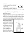
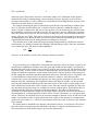
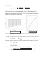
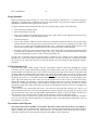
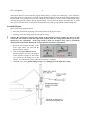
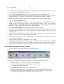
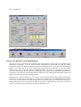
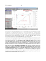
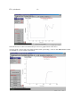
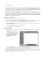
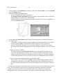
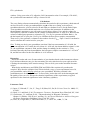
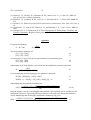
Thermometric Titration of ß-Cyclodextrin1
Microcal Isothermal Titration Calorimeter
Purpose: Determine the stoichiometry, equilibrium constant, and enthalpy of binding of ßcyclodextrin and the sodium salt of 2-naphthalene-sulfonic acid. This reaction is a good example
of a guest-host complex.
Introduction
Titrations can be done in a solution calorimeter2. The temperature of the vessel or heat flow to
the vessel is monitored as a function of added titrant. Such titrations are called thermometric
titrations. Thermometric titrations have become a commonly used method for analytical2 and
reaction enthalpy determinations3. Thermometric titrations have become especially important in
studies of protein and nucleic acid binding. For example, the enthalpy of binding of an inhibitor
to an enzyme is a common determination. In this lab we will study the binding of a cyclicpolysaccharide to the sodium salt of 2-naphthalene-sulfonic acid.
The polysaccharide is ß-cyclodextrin, ß-CD. Cyclodextrins are often used as active site analogs
for enzymes. Cyclodextrins are used to aid the absorption of drugs in the body. Other uses for
cyclodextrins include the petroleum industry for separating aromatic hydrocarbons and in
agriculture to reduce volatility of insecticides. Cyclodextrins are natural products produced by
bacteria from starch. ß-CD is made from seven D(+)-glucopyranose units linked through α-(1>4) glycosidic bonds4, Figure1.
OH
O
O
HO
OH
O
HO
15.4Å
OH
O
OH
O
HO
HO
6.5Å
OH
O
O
HO
O
HO
7.8Å
HO
HO
O
OH
HO
HO
HO
O
O
HO O
O
HO
HO
O
OH
Figure 1. ß-cyclodextrin (cycloheptaamylose).
In aqueous solution the CH bonds on the rings point inward producing a hydrophobic cavity
inside a cylinder of diameter 15.4 Å. The OH groups extend from the top and bottom of the
cylinder, providing sites for strong hydrogen bond formation. On average about 11 water
ITC-cyclodextrin
-2-
molecules fit inside the cylinder. The cavity volume is 0.14 mL/g.
O
O
Cyclo-dextrins bind with a wide variety of substances. Such
S
complexes are examples of guest-host complexes, where
O
cyclodextrin is the host.
At pH 7.2, 2-naphthalene-sulfonic acid is predominately in its
deprotonated form, Figure 2 (pKa= 0.6). 2-Naphthalene sulfonate Figure 2. 2-Naphthalene
sulfonate ion.
is expected to bind to ß-CD because it has a hydrophobic side
chain that will fit into the cyclodextrin cavity, while the -SO3- group can participate in hydrogen
bonds with the sugar OH groups. The reaction stoichiometry is not known, however, the binding
is probably 1:1 based on the size of the cavity:
ß-CD + naphthaleneSO3- → [ß-CD...naphthaleneSO3-]
1
Also remember that some water molecules originally in the cavity will be excluded in the
complex. This change in the number of water molecules in the cavity has an important effect on
the binding enthalpy and entropy1.
The analytical sensitivity of thermometric titrations is linearly related to concentration, in
contrast to the logarithmic relation to concentration that exists for many other analytical methods,
e.g., potentiometric methods. A linear relation is an advantage when very dilute solutions or
solutions with high concentrations of interfering ions are being analyzed. For example, pH
titrations of pyridine at concentrations below 0.05 M give poorly defined end points, while the
end point of a thermometric titration is well defined.
An isothermal titration calorimeter directly measures heat evolved or absorbed in liquid
samples as a result of mixing precise amounts of reactants. A spinning syringe is utilized for
injecting and subsequent mixing of reactants.
Sample and reference cells are accessible for
filling and cleaning through the top of the
unit. The sample cell is on the right as one
faces the front of the unit.
A pair of identical coin shaped cells is
enclosed in an adiabatic Outer Shield (Jacket)
to shield the system from fluctuations in the
temperature of the room. Access stems travel
from the top exterior of the instrument to the
cells. Both the coin shaped cells and the
access stems are totally filled with liquid
during operation. This requires approximately
1.8 ml. per cell even though the working
volume of the cell is only 1.4 ml
Temperature differences between the
reference cell and the sample cell are
measured, calibrated to power units and
displayed. In this respect, the instrument
operates in a similar fashion to differential
scanning calorimeters, DSC. The data
channel is referred to as the DP signal, or the
ITC-cyclodextrin
-3-
differential power between the reference cell and the sample cell. Calibration of this signal is
obtained electrically by administering a known quantity of power through a resistive heater
element located on the cell. This calibration corresponds to determining the heat capacity of the
calorimeter in other forms of calorimetry.
The syringe containing the guest is titrated (injected) into the cell containing a solution of the
host. An injection which results in the evolution of heat (exothermic) within the sample cell
causes a negative change in the DP power since the heat evolved chemically provides heat that
the calorimeter is no longer required to provide. The opposite is true for endothermic reactions.
Since the DP has units of power, the time integral of the peak yields a measurement of thermal
energy, ∆H (just as in DSC). This heat is released or absorbed in direct proportion to the amount
of binding that occurs. When the host in the cell becomes saturated with added guest, the heat
signal diminishes until only the background heat of dilution is observed.
…The titration curve is then analyzed using non-linear fitting models to calculate the reaction
stoichiometry (N), binding constant (K), enthalpy (∆rH) and entropy (∆rS). Since the calorimeter
is at constant pressure, the molar reaction enthalpy is
Qrx
∆rH = n
2
rx
where nrx is the number of moles of the limiting reactant in solution.
Theory
A typical titration curve obtained for a thermometric titration is shown in Figure 4 (left). In our
experiment, 2-naphthalene sulfonate ion is the guest and is added as the titrant. Cyclodextrin is
the host and starts in the reaction vessel. Water is used for the reference cell. The titration is done
in discrete steps. A small volume of titrant is added and then system transfers heat to or from the
sample cell until the temperature of the sample and reference cell are equalized. The integral of
the DP signal then equals the total heat transferred in this step. Then the process is repeated with
a second addition of titrant, and so on until the titration is complete. After the titration is
complete, the system will automatically plot the raw data, generate a baseline for the raw data,
integrate all peaks, and display the integration results in the Delta H window. As the titration
proceeds, the titrant that is added increases the total volume of the solution, which pushes some
of the solution up into the stem of the reaction vessel. Once the solution is pushed into the stem
any unreacted host will no longer be available for reaction with the guest. This dilution effect is
calculated and the Delta H is calculated using these changes. The effects of dilution and
exclusion of solution from the sample cell are small in this experiment. Please see the Microcal
documentation for a careful treatment of these effects. For our calculations, we will ignore these
effects. Therefore, this Delta H plot can be treated as though no dilution occurs for the host in the
sample cell. In other words, we approximate the total volume of the solution as constant and as
equal to the cell volume, Vcell. The total concentration of the host, [H]t, is therefore also assumed
to be constant.
The titrant must be standardized so that the concentration, Mguest, is well known. We wish to
know the number of guest molecules that bind to the host to verify the stoichiometry in Eq. 1.
The horizontal axis of the Delta H plot is given as the Molar Ratio:
ITC-cyclodextrin
-4-
Mguest Vguest
[G]t moles guest
Molar Ratio = r = [H] = moles host = M
t
host Vcell
3
where the M's are molar concentrations and Vguest is the volume of added guest and Vcell is the
volume of the sample cell, which holds the host. We only have a rough estimate of the Mhost,
because the extent of hydration of ß-CD is variable. Therefore, the equivalence point of the
titration won't occur exactly at a Molar Ratio of 1 or 2. However, once we have an approximate
value for N, we will round to the nearest integer.
Raw ITC Data Window
DeltaH Window
Figure 4. A typical thermogram for a simple titration (left). An exothermic reaction is illustrated.
The shape of the titration curve can be calculated using the guest-host equilibrium expression:
G+H→
← HG
[HG]
K = [H][G]
4
Assume that you have a solution with a total concentration of guest, [G]t, and host, [H]t, with
[G]t = Mguest Vguest/Vcell
then the mole balance equations are:
[G]t = [G] + [HG]
[H]t = [H] + [HG]
5
6
7
From Eqs. 4, 6, and 7, the concentration of guest-host complex is given by:
(1+K([H]t+[G]t)) - (1+K ([H]t+[G]t))2 - 4K2[H]t[G]t
[HG] =
2K
8
ITC-cyclodextrin
-5-
Using the mole ratio of the added guest to host (see Appendix for the derivations):
(1+K[H]t (1+r)) - (1+K[H]t (1+r))2 - 4K2[H]t2 r

[HG] = [H]t 
2K[H]t


9
The change in number of moles of guest-host complex after an addition of titrant can then be
determined by the change in number of moles of guest-host complex for the current step minus
the moles present during the previous step:
nHG,n = [HG]n Vcell – [HG]n-1 Vcell
10
where n is the current step number. The heat transferred to the system after an addition of titrant
is then given by the change in number of moles of the reaction
qn = nHG,n ∆rHm
11
where ∆rHm is the enthalpy change for the reaction. The vertical axis of the Delta H plot is scaled
to give a convenient range in units of kcal/mol of injected titrant:
qn 1kcal
qn,m = n 1000cal
add
12
where nadd is the number of moles of added titrant at each step. Eqns 8-12 are then used in nonlinear curve fitting to calculate K and ∆rHm. Since none of the reactants and products are gasses,
owe can assume ∆rHm = ∆rHm.
Once the equilibrium constant and reaction enthalpy are known, it is straightforward to
calculate ∆rG°m and ∆rS°m from:
∆rG°m = – RT ln K
∆rG°m = ∆rH°m – T ∆rS°m
13
14
Procedure
Prepare the solutions: Place about 2 mL of 25.0 mM 2-naphthalene-sulfonate in pH 6.9 buffer
and about 2 mL of 2.5 mM ß-cyclodextrin in pH 6.9 buffer in plastic degassing tubes.
Power Up the System
Power up the Computer Controller and VP-ITC, doing the following steps in order.
1. Turn on the computer controller. The VP-ITC power switch must be off.
2. Once the computer controller is on and Windows is running, turn on the power switch at the rear
of the VP-ITC.
3. Launch the VPViewer application by double clicking its icon on the
Windows desktop or from the Windows taskbar by selecting Start :
Programs : MicroCal’s VPITC : VPViewer ITC.
ITC-cyclodextrin
-6-
Degas Samples
Begin by degassing (with stirring) ca. 2 ml of the guest and host solutions for ca. 5 minutes using the
ThermoVac. The degassed cyclodextrin will be the solution that will go into the sample cell and the 2naphthalene-sulfonate will be placed in the syringe.
To degas solutions before placing into the cells or injection syringe, please do the following.
•
Turn on the Power Main Switch.
•
Set the temperature at 18.4°C.
•
Place your solution to be degassed into a plastic tube, add a small stir bar and place the tube into one
of the open cylinders of the Tube Holder insert.
•
Turn the stirring on.
•
Turn on the vacuum. Push the switch to the left to manually control the time for the vacuum. Start
with the bleeder valve open. Slowly close the bleeder valve. If excessive bubbling occurs that could
boil over your sample you may adjust the bleeder valve. Turning the adjusting knob clockwise will
increase the vacuum while a counterclockwise turn will decrease the vacuum strength.
•
Place the Vacuum cap on top of the sealing o’ring. The sound of the vacuum pump will change pitch
to indicate the vacuum has sealed the Cap to the o’ring. Once the vacuum has sealed, the Vacuum
Cap will be held firmly in place, till the vacuum pump shuts off.
For the first 30 seconds after the vacuum pump is turned off, the vacuum in the sample degassing
chamber may remain fairly tight making the removal of the Vacuum Cap difficult. During this period,
the easiest way to release the vacuum is to open the bleeder valve by turning the adjusting knob counterclockwise.
Fill the Sample Cell
Load the 2.5ml glass filling syringe with the cyclodextrin solution, and while holding the syringe
vertically, tap the syringe bottom after loading so all bubbles float to the top surface. Enter the needle
into the sample cell entry tube (this is the center hole located to the right of the reference entry hole) and
carefully slide the needle down the tube until it just touches the bottom of the cell. Lift the syringe so that
the needle end is just off bottom (about 1 mm), then slowly depress the plunger so that the cell fills from
the bottom up. After ca. 1.8 ml of the solution has been entered, you will be able to see the solution come
to the top of the small entry tube. Once you see the liquid level rise above the top of the access tube,
depress the plunger very quickly 1-3 times to deliver abrupt bursts of ca. 0.25 ml. The purpose of these
last bursts is to dislodge any bubbles, which might be clinging where the entry tube joins the cell. Gently
but rapidly wiggle the syringe around the cell, while not touching the bottom of the cell, to dislodge any
further bubbles.
The reference cell is kept filled with water. You won't need to touch the reference cell. There is no
need to refill the reference cell with each experiment. A water reference may be good for a week or two
with no attention, if the water was thoroughly degassed before filling. To prevent sample overflow into
the reference cell, a reference plug is used to cap the reference cell access tube after filling.
Now that the cells are filled, it is a good time to check the VP-ITC thermostat temperature and make
sure it is set to the desired run temperature of 25 degrees. If the current thermostat temperature is not set
to 25 degrees, set it now.
Precautions with Pipettes
The long needle and stir paddle on the pipette injection syringe must not be bent even slightly or
baseline stability will be compromised. Exercise care at all times in the handling of the pipette syringes.
When removing the pipette from the instrument after an experiment ends ensure that the needle is
concentric with the access tube until the end of the stir paddle is clear of the hole.
ITC-cyclodextrin
-7-
The Pipette Stand is used to hold the pipette during filling, or merely for safekeeping. Users should be
aware that damage to the pipette injection syringe needles might be incurred when placing them into the
Pipette Stand. It is good practice pay close attention to the bottom tip of the syringe needle paddle when
inserting the injection syringes into the Pipette Stand. Do not place the pipette assembly into it's stand
until you are sure that there is clearance between bottom tip of the syringe paddle and the filling tube.
Load the Pipette
Please refer to the diagrams below.
!
•
Place the guest-titrant degassing vial into the bottom of the pipette stand.
•
Carefully, insert the auto-pipette into the pipette stand.
Caution: Be careful not to hit the long needle of the injection syringe against any object, as this
could cause the needle to bend and expel some solution from the syringe and result in a poor first
injection for the experiment. If the long needle is bent far enough it may cause a permanent
deformation in the needle making the syringe unusable for future experiments.
•
Select the ITC Controls window. In the
lower right corner you will find the
Pipette Controls button.
•
Click on the Open Fill Port button.
The auto-pipette will move the plunger
of the injection syringe till the Teflon
tip is just above the filling port of the
syringe. You should hear a beep when the movement is complete.
•
Attach the tube of the plastic filling syringe to the filling port of the injection syringe.
Guest-titrant degassing vial
ITC-cyclodextrin
-8-
•
Slowly withdraw the plunger of the plastic filling syringe to draw up the titrant solution till you see
the solution exit through the top filling port.
•
Click on the Close Fill Port button as soon as you see the liquid exit the top filling port.
The pipette will lower the plunger of the injection syringe till the white Teflon tip is completely
below the filling port (ca. 4mm). You should here a beep when the movement is complete.
•
Remove the hose of the plastic filling syringe from the filling port of the injection syringe.
•
Click on the Purge->ReFill button.
The auto-pipette will depress the plunger of the filling syringe to inject the sample back into the
filling test tube, then raise the plunger to refill the injection syringe. When the movement is
complete the tip of the injection syringe will be positioned to its original position, just below the
filling port. A beep will indicate the completion of the movement.
•
Click on the Purge->ReFill button again to repeat the purge/refill action.
The purpose of both purge/refill procedures is to dislodge any air bubbles from inside walls of the
injection syringe (which may have occurred during the first filling) and expel them back into the
titrant solution.
•
Carefully remove the pipette from its stand by picking it straight up till the glass barrel of the
injection syringe is above the top part of the pipette stand.
•
Carefully move the pipette so that it is directly above the center positioned sample cell access tube
(this is the hole on the right).
•
Carefully insert the pipette into the sample cell access tube.
Watch the end paddle of the long needle to insure it is inserted directly into the access hole, hold the
pipette vertical and slowly lower the pipette. When the pipette is almost completely inserted you may
have to push down slightly to compensate for the resistance of the rubber o’ring to seat the pipette.
Enter the Run Parameters into VPViewer
•
Select the Load Run File button from the main window buttons.
•
Select the CH341CD.inj run parameters file and click Open.
The ITC Controls window will show run parameters for the water experiment (see below).
•
Enter a filename. Use no spaces or punctuation in the file name
•
Click on the Setup/Maintenance tab and set the data file path to
“C:\\VPITC\data\twshattu\ITC Data”
•
Check that the Reference power is set to 120 uCal/sec.
•
Enter the concentrations for the cyclodextrin in the Cell Concentration dialog box. This
concentration will be about 2.5 mM. Enter the concentration for the guest in the Syringe
Concentrations box. The titrant concentration will be about 25. mM.
ITC-cyclodextrin
•
-9-
Select the Start button, to start the experiment.
Observe the Baseline while Equilibrating
At the start of the experiment the instrument may rapidly bypass certain stages of operation. If the
instrument’s temperature is at the selected starting temperature the instrument will skip the seeking
temperature and pre run thermostatting phase and move immediately on to the final baseline equilibration
phase. If your instrument is not at the entered starting temperature you may have to wait an extended
period of time prior to the final baseline equilibration state. The states of operation are displayed in
VPViewer and Origin at the top, right in red. Displayed below is data from an instrument that started at a
temperature lower than the desired experimental temperature and is showing the temperature rising to 30
degrees and stabilizing at the starting temperature.
Displayed above are three different Y-axis scales with four different data sets being plotted in the graph.
Each Y-axis is plotted in its own layer (see Origin User’s Manual for more information about layers).
You can see the layer button located in the upper left corner of the graph. The black number on the gray
button indicates the active layer while the inactive layers have white numbers. You may set a layer as
active by clicking on the layer button or on the corresponding Y-axis.
ITC-cyclodextrin
-10-
The Y-axis on the left is colored blue and the data set plotted in this layer (also colored blue) is the DP
data (DP data is the differential power between the reference and sample cell). When Pre-stirring
equilibration is first started the data may not be visible on the graph. One can click on the Auto-View 2
button to center the current data point with a Y-axis full scale of 1. When the cell has equilibrated in the
Pre-stirring mode you may want a closer look at the data, so click on the Auto-View 1 button. This will
put the current data point at the center of the graph with a Y-axis full scale of 0.1.
You may notice that when the graph first appears in Origin, the DP data display box in VPViewer’s main
window has the values displayed in red. Once VPViewer determines that the cell has equilibrated in the
Pre-stirring mode, the data display will turn to green. This means that the cell is ready to enter the
stirring mode of equilibration. Since Auto Start in the ITC Equilibration Options group was enabled
in the ITC Controls window, VPViewer will automatically start the stirring and apply power to the
reference cell, moving on to the next state of the equilibration process. If this option was not selected the
DP value that turned green becomes a button that will move the instrument to the next state when it is
selected.
When VPViewer starts the Final Baseline Equilibration it starts the stirring and applies power to the
reference cell. The amount of power applied to the reference cell is determined by what you entered into
the Baseline Position (uCal/sec) text box located in ITC Controls window. For this tutorial we entered
5 for the Baseline Position, you may see that there may be an initial decrease in the DP power (due to the
added frictional energy in stirring), but then the DP values will increase because of the power applied to
the reference which forces the feedback system to apply power to the sample cell to compensate and
maintain a temperature balance. The effect of this heat disturbance will take a few minutes for a new
equilibration level with the final DP values being close to 5.
ITC-cyclodextrin
-11-
Select the Rescale to Show All button and you will see a graph similar to the above.
You may want a closer look at the final baseline before proceeding. Click on the Auto-View 1 button.
You should see a view similar to that below.
ITC-cyclodextrin
-12-
When VPViewer determines that the Final Baseline has equilibrated properly, the display in the DP box
will turn from red to green. Since Auto was checked in the ITC Equilibration Options group,
VPViewer will automatically start the experiment. (If the automatic mode was disabled you would now
need to double-click anywhere in the DP display box, to start the experiment).
The experiment will begin, the DP display box will turn from green to black and the display title will
read Pre-Titration delay and then print the volume of solution that is left in the syringe. The PreTitration Delay is required for an initial baseline for the first injection of the experiment. The time
period for this initial baseline was entered in the Initial Delay text box located in the ITC Equilibration
Options group of the ITC Controls window.
Observing the Experiment
After a few injections you may want to view the injection peaks.
Please note: While running VPViewer and switching between application you may sometimes see gaps
in your data or no data being plotted, select Window:Refresh to see all the plotted data.
•
Select Auto View 2 and you should see a plot similar to Figure 4. You may also want to get an even
closer look at the baseline.
•
Click on Auto View 1 button to see an expanded view.
•
Allow all 29 injections to be completed.
Analyzing the Data
•
Minimize the VPViewer application by clicking on the Minimize button in the upper right corner of
the window.
•
Open Origin for data analysis, by
selecting Start, from the Taskbar,
then select Programs:MicroCal
Origin:MicroCal Inc. ITC. You
should see the ITC raw data
template.
•
Click on the Read Data button, to import your VP-ITC data into the plot window. Find your way to
the data folder and select the file containing your data, and click Open.
Origin will automatically plot the raw data, generate a baseline for the raw data, integrate all peaks, and
display the integration results in the Delta H window, as in Figure 4. Origin automatically plots
concentration-normalized areas (kcal per mole of injectant).
ITC-cyclodextrin
•
•
•
-13-
Click anywhere on the DeltaH plot window to make it the active window. Or select DeltaH
from the Window menu.
Click on the One Set of Sites button.
A new command menu display bar appears.
The Fitting Function Parameters dialog box opens, showing initial values for the three
fitting parameters for this model - N, K, and H.
Origin initializes the fitting parameters, and plots an initial fit curve (as a straight line, in
red) in the DeltaH window.
Click 1 Iter. or 10 Iter. button in the Fitting Session dialog box to control the iteration of
the fitting cycles.
Click 1 Iter. to perform a single iteration, 10 Iter. to perform 10 iterations. It is usually
necessary that the 10 Iter. command be used more than once before a good fit is
achieved. Repeat this step until you are satisfied with the fit, and Chi^2 is no longer
decreasing. Note that the fitting parameters in the dialog box update to reflect the current
fit.
To hold a parameter constant:
The Vary? column in the Fitting Session dialog box contains three checkboxes, one
associated with each fitting parameter. If a box is check marked, Origin will vary that
parameter during the fitting process in order to achieve a better fit. To hold a parameter
constant during iterations, click in the box to remove the checkmark from the checkbox.
To copy and paste the fitting parameters to the DeltaH window:
Once you have a good fit, click on the Done.. button and the fitting parameters will be
automatically pasted into a text window named Results and to the DeltaH window in a
text label. Position this label just as you want the fitting parameters to appear. Print the
plot.
To make your spreadsheet calculations easier, it will be best to have the stoichiometric ratio, N,
be one. The reason that N may not be one is that the concentration of the beta-cyclodextrin
solution is not accurately known. We can use the results of your titration to calculate the
concentration of the cyclodextrin solution. Click on the Concentrations button in the main
ITC-cyclodextrin
-14-
window. Using your value of N, adjust the Cell Concentration value. For example, if N=0.983,
the cyclodextrin concentration is off by a factor of 0.983.
Calculations
The curve fitting software automatically calculates the results for this experiment, which ruins all
our fun. However, to help you understand the results
o- of the curve fitting, write an Excel
spreadsheet that uses your fit values for K and ∆rHm to calculate fit curve for the Delta H plot.
Your spreadsheet results should match the curve fit from the instrument. In addition to the
thermodynamic parameters, you will need to specify Mguest, Mhost, Vcell, and the volume for
each injection. Generate a column for the volume of titrant added for 35 steps or so. Based on the
volume of added guest generate a column for [G]t. Use Eq 3 to generate the Molar Ratio, r, for
the horizontal axis of your plot. Use Eq 9 to calculate the host-guest complex concentration.
Then use Eq. 10 to generate a column for the number of moles, nHG,n. Eqns 11 and 12 can then be
used to calculate the vertical axis for your plot.
Hint: To help you check your spreadsheet, note that if the host concentration is 2.50 mM, the
guest concentration is 25.0 mM, the cell volume is 1.4389 mL, the titrant addition volume is 10.0
µL, the equilibrium constant is 2000, and the change in enthalpy for the reaction is -7500
kcal/mol, then after the first titrant addition: the host-guest complex concentration is 1.4333x10-4
M, and the heat effect for the first addition is -6.19 kcal/mol.
Discussion
Report the results and curve fit uncertainties of your titration based on the instrument software.
If you did more than one run, give the uncertainty for each value based on your replicate trials.
Calculate the uncertainty in the reaction entropy. How well do your results match the literature
values?1
What do the stoichiometry and ∆rH°m, ∆rG°m, and ∆rS°m of the reaction tell you about the
complex? Why does the complex form? Please include a copy of your experimental curve fit,
your spreadsheet, and a full page plot from your spreadsheet. What do you think is the
predominant error for this experiment? To answer this, look at the noise in the thermogram and
the quality of the curve fit. Discuss the chemical significance of the experiment (see typical
questions for the chemical significance in the Laboratory syllabus).
Literature Cited
(1) Inoue, Y; Hakushi, T.; Liu, Y.; Tong, L-H; Shen, B-J; Jin, D-S J.Am. Chem. Soc. 1993, 115,
475-481.
(2) Bark, L. S. and Bark, S. M., Thermometric Titrimetry, Pergamon Press, Elmsford, NY, 1969.
(3) Christensen, J. J., and Izatt, R. M., "Thermochemistry in Inorganic Chemistry,"
Chapter 11 (Editors: Hill, H.A.O., and Day, P.), in Physical Methods in Advanced Inorganic
Chemistry, Interscience Publishers, New York, NY, 1968.
(4) Diaz, D.; Vargas-Baca, I.; and Garcia-Mora, J., J. Chem. Ed. , 1994, 71, 708.
ITC-cyclodextrin
-15-
(5) Hansen, L. D. ; Kenney, D. ; Litchman, W. M. ; and Lewis,E. A., J. Chem. Ed., 1971, 48
(12), 851-852 for a similar experiment.
(6) Hansen, L. D., Litchman, W. M., Lewis, E. A., and Allred, R. E., J. Chem. Educ., 1969, 46,
876.
(7) Rossini, F. D., Editor, Experimental Thermochemistry, Interscience, New York, NY, 1956, p.
30.
(8) Christensen, J. J., Izatt, R. M., Hansen, L. D., and Partridge, J. A., J. Phys. Chem., 1966,70,
2003.
(9) Eatough, D. J., J. J. Christensen, R. M. Izatt, Experiments in Thermometric Titrimetry and
Titration Calorimetry, Brigham Young University Press, Provo, Utah, 1974; p. 25.
Appendix
For guest-host binding:
G+H→
← HG
[HG]
K = [H][G]
15
The mole balance equations are:
[G]t = [G] + [HG]
[H]t = [H] + [HG]
16
17
or solving Eqs. 16 and 17 for the free guest and host concentrations gives:
[G] = [G]t - [HG]
[H] = [H]t - [HG]
18
19
Substitution of the mole balance expressions into the equilibrium constant expression:
[HG]
K = ([H] - [HG])([G] - [HG])
t
t
20
Cross-multiplying and rearranging gives a quadratic expression:
K ([H]t - [HG])([G]t - [HG]) = [HG]
21
K[HG]2 - (1 + K([H]t + [G]t) [HG] + K[H]t [G]t = 0
22
Substitution into the quadratic formula gives:
[HG] =
(1+K([H]t+[G]t)) ± (1+K ([H]t+[G]t))2 - 4K2[H]t[G]t
2K
23, (8)
Only the negative root gives meaningful concentrations. This equation can be used directly for
calculations. However, expressing [HG] as a function of the mole ratio during the titration is
useful. Multiplying and dividing the equilibrium constant by [H]t gives:
[HG] =
(1+K[H]t (1+[G]t/[H]t)) - (1+K[H]t (1+[G]t/[H]t))2 - 4K2[H]t2 [G]t/[H]t
2K[H]t/[H]t
23
ITC-cyclodextrin
-16-
[G]t
The mole ratio of the added guest to host is r = [H] :
t
(1+K[H]t (1+r)) - (1+K[H]t (1+r))2 - 4K2[H]t2 r

[HG] = [H]t 
2K[H]t


24, (9)
Eq. 24 is applicable to any chemical equilibrium with similar stoichiometry, e.g. 1:1 binding and
acid base reactions. Similarly, the free concentrations of host and guest can also be calculated9:
-(1+K[H]t (1-r)) + (1+K[H]t (1-r))2 + 4K[H]t r

[G] = [H]t 
25
2K[H]t


-(1+K[H]t (r-1)) + (1+K[H]t (r-1))2 + 4K[H]t

[H] = [H]t 
2K[H]t


26
Or the mole balance equations, Eqs. 18 and 19, can be used with Eq. 24 to calculate the free
guest and host concentrations.