1
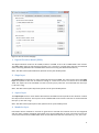
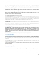
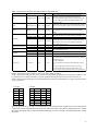
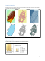
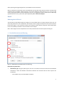
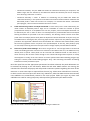
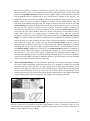
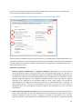
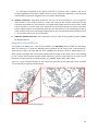
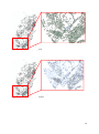
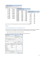
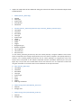
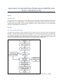
Automatic Overland Flow Delineation (AOFD) tool - User's manual (v2.0) By João P. Leitão (December 2009) – Updated by Susana Ochoa-Rodríguez (December 2013) Part I Introduction This document aims at helping users run the Automatic Overland Flow Delineation (AOFD) tool developed by Maksimovic et al. (2009). AOFD is a GIS (Geographic Information Systems) tool which generates 1-dimensional (1D) models of the overland network (or urban surface) based on an accurate digital elevation model (DEM) of the study area. Part II Structure of the AOFD tool The AOFD tool comprises several individual steps through which the 1D model of the overland flow network is created. These steps are illustrated in Figure 1. The output files generated by the AOFD tool are ready to be imported into Infoworks CS or SIPSON in order to create a 1D model of the surface. Using these software packages, the 1D surface model can be coupled with a model of the sewer system, thus creating a 1D-1D dual-drainage model suitable for simulating urban pluvial flooding. Figure 1: Flowchart of the Automatic Overland Flow Delineation (AOFD) tool (Leitão et al., 2009). 1 Part III AOFD executables: location and launching of the tool The AOFD tool is made up of a number of executable files located in a main folder which in turn contains several subfolders (see Figure 2). Users must store the main folder in a location with a path as short as possible; ideally, directly in one of the computer’s main drives (e.g. C:\ or D:\). The main folder can be re-named, but it is advisable to keep the name short and to avoid using special characters. Long paths and folder names may cause the execution of the AOFD to crash. The names of the internal subfolders and of the executable files cannot be modified. The AOFD tool is a stand-alone and portable application (i.e. it does not require installation). Once the main folder containing the executable files is stored in the computer (as explained above), the AOFD tool can be launched simply by double clicking the SurfFlowNetwork.exe file (see Figure 2). When launching it, the AOFD graphic user interface (GUI) pops up. The GUI comprises 5 tab pages, each of which can be used for different purposes, as described in the following sections. Figure 2: File conversion tab page. Part IV Preparation of input data All files required to run the AOFD tool are in IDRISI 16bit vector and/or raster format. The AOFD tool includes an interface to convert ESRI ASCii format files to IDRISI 16bit raster format files, and vice-versa. In addition, it includes a tool for converting ESRI shapefile format to IDRISI 16bit vector format, and vice-versa. Figure 3 shows the interface for file conversion. The input files required to run the AOFD tool are the following: • Digital Elevation Model (DEM) • Slope layer • Aspect layer • Manholes layer • Catchment boundary layer • Cover layer (the same as catchment boundary) • Buildings layer • Project file In the following sections each of these files is described. 2 Figure 3: File conversion tab page. 1. Digital Elevation Model (DEM) The digital elevation model can be a DEM, a DTM or a DTMb. It has to be in IDRISI 16bit raster format. The IDRISI 16bit raster format comprises two files: (i) a *.doc and a *.img file (these two files are obtained when converting ESRI ASCii files to IDRISI 16bit raster format using the tool described above). Note: The data values of the DTM raster file have to be of the double format. 2. Slope layer The slope layer corresponds to a raster dataset derived from the DEM. The value of each cell of the slope layer corresponds to the rate of maximum change in z-value from the cell. Its format has to be IDRISI 16bit. The slope has to be calculated in meter by meter [m/m]. Two files are associated with this layer (*.doc and *.img). Note: The data values of the slope raster file have to be of the double format. 3. Aspect layer The aspect layer is also a raster dataset derived from the DEM and corresponds to the direction in which the slope of each cell faces. This layer has to be in IDRISI 16bit raster format. Two files are associated with this layer (*.doc and *.img). Note: The data values of the aspect raster file have to be of the double format. 4. Manholes layer Information about manholes is essential to generate an overland flow network that can be integrated with the sewer network. Manhole information has to be provided both in vector and raster format. The vector format has to be the IDRISI 16bit vector format which has two files associated: (i) *.vec, and *.vdc. 3 The raster format is the IDRISI 16bit raster format where each manhole must be represented by its ID (which must be an integer and must be the same ID used in the vector file). Cells representing the catchment boundary (including points inside the catchment) must have a zero (0) value, and cells outside the catchment must be assigned a -1 value. Associated with manhole information, there are two more files (*.csv and *.ntt) in text format which create a correspondence between the integer manhole IDs in the raster and vector files, and the manhole IDs in the hydraulic model (e.g. Infoworks) (see Figure 4). Notes: (i) In the manhole raster file, each cell can only have one manhole; (ii) The data values of the manholes raster file must be of the double format. 5. Catchment boundary and cover layers The catchment boundary has to be provided in both vector and raster IDRISI 16bit format. Thus, four files have to be present in the Inputdata folder: *.vec, *.vdc, *.doc and *.img. The vector file has to be of polygon type and the polygon ID must be one (1). In the raster file, cell values outside the catchment area must have value minus one (-1) and cells inside the catchment must have value one (1). The cover layer is simply a copy of the four catchment boundary files; the only difference between them is the file name. Notes: (i) Raster files of the boundary and cover are integer type; (ii) Cover file is necessary (useful for SIPSON and BEMUS models) and equal (a copy of the catchment boundary files). 6. Buildings layer The buildings layer contains information about the location of buildings within the study area. It has to be provided in both vector and raster IDRISI 16bit format. Thus, four files have to be present in the InputData folder: (i) *.vec, *.vdc, *.doc and *.img. The vector file has to be of the polygon type. In the raster file, cells inside buildings must be assigned a value of one (1) and cells outside buildings must be assigned zero (0). Note: The data values of the buildings raster file have to be of the integer format. 7. Project file (*.pro) This file, in text format, summarises key characteristics of the study area and of the input files to be used in the analysis. It provides the main instructions required to run the AOFD tool, including names of input files, extent of study area, elevation range, grid size, and number of rows and columns in the input files of raster type. In order to generate the project file, AOFD developers will provide users with a template they can customise to their own study area. If the information in this file is incompatible with the characteristics of the input files, the execution of the AOFD tool will fail. Summary of input files The table below provides a summary of the input files, including their format, data type and a brief description. 4 Table 1: Summary of the input files required to run the AOFD tool INPUT DATA FILE FORMAT (REQUIRED FILES) DATA TYPE DEM IDRISI 16 bit Raster *.doc, *.img Double SLOPE IDRISI 16 bit Raster *.doc, *.img Double ASPECT IDRISI 16 bit Raster *.doc, *.img Double IDRISI 16 bit Raster *.doc, *.img Integer DESCRIPTION/EXPLANATORY NOTES Digital Elevation Model. It is important to represent the buildings in this file: the buildings must be given an elevation significantly higher than that of the boundary cells (this can be done by processing the DEM or DTM in a GIS software package) Derived from the DTM. Can be generated with a GIS software package. The slope must be given in [m/m] (dimensionless) Aspect is the direction in which a slop faces. It can be derived from the DTM and can be generated with a GIS software package Manholes are represented by their ID. Cells representing catchment boundary = 0, outside catchment boundary = -1 IDRISI 16 bit Vector *.vec, *.dvc MANHOLES Creates correspondance between the integer manhole IDs in the raster and vector format files (the manhole IDs in both Text *.csv, *.ntt Text (string) files should be the same, but the software needs these correspondence files to run). IDRISI 16 bit Raster *.doc, *.img Integer Cells outside catchment = -1, inside = 1 CATCHMENT BOUNDARY IDRISI 16 bit Vector *.vec, *.dvc Polygon type, polygon ID = 1 IDRISI 16 bit Raster *.doc, *.img Integer COVER Copy of catchment boundary IDRISI 16 bit Vector *.vec, *.dvc IDRISI 16 bit Raster *.doc, *.img Integer Value inside buildings = 1, outside = 0 BUILDINGS IDRISI 16 bit Vector *.vec, *.dvc PROJECT FILE Text format *.pro Text A template of this file must be provided by the AOFD developers. The user must edit this file manually in order to show the following: - Names of input files - Extent (coordinates, left, right, top and bottom) of study area - Elevation range (maximum and minimum "z" values) - Number of rows and columns of the input raster files - Cell size of the final grid (to match that of the raster layers) NOTE 1: All raster files must have the same extent and cell size NOTE 2: The structure of the manhole *.csv and *.ntt files is shown in Figure 3. NOTE 3: Input files can be given any name, but this must be updated accordingly in the project file. However, users are advised not to use special characters in the files name and to keep file names shorter than 10 characters. NOTE 4: The project file can be given any name (following the above recommendations), as long as the file extension (.pro) is preserved. *.csv file R1 V1 R2 V2 R3 V3 . . . . . . . . Rn Vn *.ntt file R1 V1 R2 V2 R3 V3 . . . . . . . . Rn Vn FFFF FFFF FFFF . . . . FFFF 1 1 1 . . . . 1 Figure 4: Structure of *.csv and *.ntt manhole files (see file description in Table 1). Ri and Vi correspond, respectively, to the manhole ID in the raster file and vector files. These IDs are usually the same in both the raster and vector files, so the first and second columns of the *.csv and *.ntt manhole files are usually the same. 5 Examples of input files Examples of some of the input files required to run the AOFD tool are shown in Figure 5. These examples correspond to the Cranbrook catchment (UK). (a) DEM (raster) (b) Slope (raster) (d) Catchment boundary & cover (vector) (e) Buildings (vector) (c) Aspect (raster) (f) Manholes (vector) Figure 5: Examples of input files for AOFD tool Organization of files The files required to run the tool AOFD have to be organized as follows: Figure 6: Organisation of input files 6 After preparing and organising the files, the AOFD tool can be executed. Notes: (i) Similar to the location of the executable file, the input files must also be stored in a location with a path as short as possible, ideally, directly in one of the computer’s main drives (e.g. C:\ or D:\) (ii) The name of the project folder can be changed, but the user is suggested to keep it short and to avoid using special characters in it; (ii) The name of the InputData folder cannot be changed. Part V Running the AOFD tool The execution of the AOFD comprises 4 stages, for each of which there is a special tab where the user can select the parameters to be considered in the analysis. These 4 stages correspond to the internal routines illustrated in Figure 1. The interfaces used for each stage are shown below, along with a brief explanation of the user-defined parameters to be considered in the analysis. Note: These stages must be completed in strict order; otherwise the execution of the tool may fail. 1. Pond delineation and filtering i ii iii Figure 7: AOFD tab for pond delineation and filtering Description of parameters: i. Delineation type: using the options given, the user can choose the area for which the overland flow delineation is done and whether interactions between the overland and the sewer systems are considered: - Entire DEM: every cell of the DEM is analysed 7 - Catchment boundary: only the DEM cells within the catchment boundary are analysed. If the DEM is larger than the catchment, the DEM cells outside the boundary will not be analysed, thus achieving a reduction in runtime. - Catchment boundary + sewer: in addition to considering only the DEM cells within the catchment boundary, in this option the interaction and relative location between manholes and delineated ponds is taken into account. For example, if a manhole falls within a delineated pond polygon, a weir connection between the two is created. ii. Pond removal using volume and depth thresholds: in most cases (even in small catchments), the initial number of identified ponds is huge and it is advisable to reduce the number of ponds (computational nodes) to an acceptable level. For this purpose, volume and depth thresholds can be defined by the user in order to filter out small depressions (recommended volume and depth filtering thresholds are provided in the user interface). This filtering routine removes some little ponds from the analysis (which satisfy both the depth and volume thresholds set by the user), but the DEM remains unchanged, thus preserving slope features required for the pathway delineation procedure. This approach is different from the standard “fill” method of the ArcGIS Toolbox, which fills all sinks (regardless of their size) with a user specified depth. In this way, little ponds (or pits) are removed, but the big ones also loose part of their storage capacity and the DEM is modified. iii. Removal of ponds inside buildings: when there are gardens or roof storage features constructed inside the building perimeter and these are reflected in the DEM of the area, the AOFD tool may identify them as ponds. These ponds can be removed and modelled instead as initial losses, in which case they will not have surface linkage to the overland drainage network (which is usually what happens in reality). If the user chooses to remove ponds located within building polygons (by ticking the ‘remove ponds inside building polygons’ box), a file containing information of building boundaries must be provided as input. Once the input files and the appropriate parameters have been selected, the pond delineation can be executed by clicking on the ‘OK’ button. While this and other AOFD routines are running, the command line interface will pop up and will provide continuous updates regarding the status of the execution. In some cases input is required from the user (e.g. ‘Please enter a blank line to continue’, in which case the user must press the ‘Enter’ key). Moreover, when the AOFD routines are executed, new subfolders are automatically created in the main project folder (see Figure 8); these new subfolders are used for storing temporary and output files generated by the AOFD routines. Figure 8: New folders automatically generated when running the AOFD tool 8 2. Flow path delineation (connectivity analysis) i ii 10-20 m 20 - 30 iii Same as DEM resolution Figure 9: AOFD tab for flow path delineation. Note: the values shown in this (with the arrows) are recommended or typical parameter values; a description of the rationale behind them is provided below. It is the user’s responsibility to choose suitable parameter values for his/her model. Description of parameters: ii. Delineation type: using the options given, the user can choose whether to consider overland pathways only between ponds (i.e. ‘pond links’ option) or also between ponds and manholes (i.e. ‘ponds and manholes linkage’ option). iii. Path delineation parameters: - Buffer radius (m): during the path delineation process it may occur that, based on the surrounding cells, the algorithm cannot find the direction of the next ‘stretch’ of the pathway (this may occur, for example, in relatively flat areas). To overcome this problem, the user may specify a distance larger than the pixel size in which the algorithm can search for the direction (gradient) of the pathway. A buffer radius between 10 m to 20 is recommended. - Number of iterations: this is a stop criterion, used in the case in which the algorithm cannot find the direction of the next stretch of a pathway. As explained above, when this happens the algorithm starts searching for the path direction gradually within the specified buffer radius; if for any reason it takes too long or a solution cannot be found, the search stops once the number of tries or iterations reaches the number specified by the user. A number of 20-30 iterations is recommended. - Consider buildings in delineation: the user can choose whether or not considering the presence of buildings in the identification of overland flow pathways. Considering buildings is strongly recommended, given that in reality buildings constitute obstacles to overland flow 9 pathways and alter their trajectory. If buildings are to be considered in the pathway delineation process, a file containing information of building boundaries must be provided as input. iv. Surface junction parameters – grid size for analysis (m): during the path delineation process, there is a possibility that two or more pathways come very close and flow parallel or nearly coincide with each other. In reality, these pathways merge and flow through a single path from the point at which they meet. This must be accounted for in the simulation model. The way in which this is done is that if two pathways are at a distance shorter than or equal to a user defined value (namely, the ‘grid size for analysis’ parameter), then they are combined into a single pathway. When this happens, a new type of computational node called ‘surface junction’ is created at the point at which the two paths meet. The recommended value for this parameter is the same length as that of the DEM pixels (e.g. if the DEM resolution is 5 x 5 m, use a grid size for analysis = 5 m). Once the input files and the appropriate parameters have been selected, the path delineation can be executed by clicking on the ‘OK’ button. 3. Estimation of pathway geometry and drainage capacity ii i 1.5 m 10 m 1/1 10-50 m (must be a multiple of the grid size) 1.5 – 3 m 0.1 – 0.25 m Approx. 5 m 1 – 3 times the grid size Figure 10: AOFD tab for cross section analysis. Note: the values shown in this figure (with the arrows) are recommended or typical parameter values; a description of the rationale behind them is provided below. It is the user’s responsibility to choose suitable parameter values for his/her model. Description of parameters: i. Estimation of channel geometry parameters: in order to model surface flow through overland pathways (using the 1D modelling approach), the following information is required: geometry of the open channel, upstream/downstream elevations (and resulting slope), and actual length of the pathway (i.e. distance between the starting and ending node of the pathway). The algorithm with 10 which this information is obtained is illustrated in Figure 11. This algorithm uses the previously extracted pathways (step 2 of the AOFD tool) and draws equi-distant cross-sections along each pathway at longitudinal intervals defined by the user (Figure 11(b)); the recommended value for the longitudinal interval is between 10 to 50 m and must be a multiple of the grid size. The algorithm then uses the surrounding DEM to estimate and average the areas of each cross-section (Figure 11(c)); to do this the DEM is inspected at regular intervals perpendicularly from the centreline of the pathway (see Figure 10). The length of these intervals corresponds to the cross section interval parameter to be defined by the user; the recommended value for it is 1 to 3 times the grid size. The maximum distance from the centreline to which the DEM is inspected (to determine the area of the cross section) corresponds to the user-defined buffer radius parameter (see Figure 10). This value should be equal to or greater than half the normal width of road (a buffer radius value of 5 m or slightly larger is recommended). Lastly, there are two more parameters related to the initial estimation of the channel geometry: the minimum and maximum depths. The minimum depth threshold corresponds to the vertical distance between the bottom and top of the cross section for which the cross section is assumed to be flat (i.e. if the depth of the cross section (see Figure 10) is smaller than the specified minimum depth, the cross section is assumed to be flat). When a cross section is assumed to be flat, a default trapezoidal cross section defined by the user (see parameter (ii)) is assigned to this pathway. The recommended value for the minimum depth is between 0.1 and 0.25 m. The maximum depth parameter corresponds to the cross-section depth above which it is assumed that a building or a similar obstacle has been encountered (i.e. if the cross-section depth is greater than the specified maximum depth, it is assumed that a building has been encountered). When the depth of the cross section exceeds the specified maximum depth, the latter is applied by default to the cross section. The recommended value for the maximum depth is between 1.5 and 3 m. ii. Default trapezoidal channel: as mentioned above, when the cross section of a pathway is deemed to be flat, a default trapezoidal section defined by the user is assigned to it. Moreover, the AOFD tool generates two sets of pathways: one with irregular cross sections, determined based on the analysis of the DEM, and another one in which all pathways are assigned the default trapezoidal channel section defined by the user. It is up to the user to decide which set of pathways is to be used for generating the 1D model of the surface. Recommended values for the default trapezoidal section (based on typical street sections) are: 1.5 m depth, 10 m width and 1/1 slope. Figure 11: Estimation of pathway geometry and drainage capacity (a) 3D DEM showing identified flow path, (b) number of cross-section lines drawn perpendicularly to path, (c) arbitrary shapes of cross sections plotted as estimated from the DEM, and (d) averaged output with two choices: trapezoidal or arbitrary shapes. (Maksimović et al., 2009). 11 Once the project file and the appropriate parameters have been selected, the cross section geometry routine can be executed by clicking on the ‘OK’ button. 4. Generation of surface flow network and creation of output files i iv ii iii Figure 12: AOFD tab for creation of surface flow network After the previous individual steps have been carried out (i.e. pond delineation, pathway delineation and estimation of pathway cross-section geometry), the last step of the AOFD is to put the pond and pathway elements together and create the 1D model of the overland. For doing this some additional parameters must be defined by the user. Description of parameters: i. Pathway hydraulic characteristics – roughness coefficient: depending on the flow-resistance formula that will be used for routing the flow on the 1D overland network model (i.e. whether it is the Manning formula or the Darcy-Weisbach equation in combination with Colebroo-White), the user can define the roughness of the overland pathways in terms of Manning’s “n” coefficient or as the absolute roughness height ks. The roughness coefficient defined by the user will be assigned uniformly to all pathways of the overland model. As most urban surfaces are covered by asphalt/concrete and roughness is usually big, a Manning “n” value between 0.015 - 0.035 and a ks value between 10 mm – 50 mm is recommended. In any case, it is up to the user to select an appropriate value for the roughness coefficient, based on the characteristics of the area under consideration. ii. Sewer interactions (manholes to ponds): the flow exchange between the overland network and the sewer system takes place at manholes and gullies and can be modelled as a weir flow (as long as free-flow conditions remain). The user is required to indicate the parameters to be used for estimating this flow. Typical values for weir coefficient and weir crest length are, respectively, 0.8 and 12 ~ 3 m (the latter corresponds to the typical perimeter of a manhole cover). However, the user is strongly suggested to determine suitable values for these parameters depending on the particular characteristics of manholes and gullies in the area under consideration). iii. Optional parameters: using these parameters, the user can choose whether or not to include an extra elevation to the surface ponds (i.e. above the level that was initially determined through inspection of the DEM). An extra elevation in the ponds adds storage volume to each of them, which may be necessary in case the water level reaches the top of the pond. Moreover, this extra elevation leads to higher gradients in the hydraulic grade line once the pond is full, thus facilitating the flow of water from the pond to the connecting surface pathways. An extra elevation of few centimetres (e.g. 5 – 10 cm) and a slope of 1/1 is recommended. iv. Additional SIPSON parameters: these parameters are only used when generating outputs suitable for SIPSON software. Output files of the AOFD tool The output of the AOFD tool is a set of files (located in the DSD folder) which contain the information about the elements (i.e. ponds and pathways) that constitute the 1D model of the overland network. These files are ready to be imported into either InfoWorks CS (Innovyze, 2012) or SIPSON (Chen et al., 2007) software packages and can be easily coupled with 1D models of the sewer system, thus allowing for the creation of 1D-1D dual drainage models. Moreover, the files can be edited so that they can be inputted into other hydraulic simulation software (e.g. SWWM, Sobek Urban, Mike Urban). Figure 13 - Figure 16 show examples of the output files generated by the AOFD tool. These examples correspond to the Cranbrook catchment (UK). Figure 13: Surface ponds shapefile (polygon) 13 Figure 14: Surface nodes shapefile (point) Figure 15: Overland pathways shapefile (line) 14 Figure 16: Text files containing information about overland ponds and pathways Part VI Importing AOFD output files into InfoWorks CS In order to import the 1D model of the overland network (generated with the AOFD tool) into InfoWorks CS and couple it with a 1D model of the sewer network, the following steps must be followed: 1. Open and check out the model of the sewer network 2. Open the Data Import Centre (under the Network menu) (see Figure 17) Figure 17: Data Import Centre – InfoWorks CS 15 3. Import the output files of the AOFD tool taking into account the tables and associated object fields indicated below: i. Nodes (Surface_Node.shp): NodeID Node type System type Ground level Flood level ii. Conduit (Surface_Estimated_Channels.shp or Surface_Default_Channels.shp*): US nodeID Link suffix DS nodeID Link type System type Length Shape_ID Width Height Roughness type Bottom roughness Top roughness US invert level DS invert level *In the ‘Surface_Estimated_Channels.shp’ file each surface pathway is assigned a different cross section which corresponds to the average area/shape of all the cross sections analysed in that specific pathway. In contrast, in the ‘Surface_Default_Channels.shp’ file all surface pathways are assigned the same cross section which corresponds to the ‘Default Trapezoidal Channel’ parameters defined by the user (see Figure 10). It is up to the user to decide which of the cross sections to use. It is important to notice that using the ‘estimated’ cross sections often causes instabilities in the hydraulic model. iii. Weir (Surface_Weir.shp): US nodeID Link suffix DS nodeID Link type System type Crest Width Height Discharge coefficient iv. Node: Storage level (UserDefined_Pond.csv): Node ID Storage level v. Node: Storage area (UserDefined_Pond.csv): Node ID Storage area 16 NOTES: The linkage between the overland and the sewer system takes place at manholes/gullies. Provided that correct manhole files (see Table 1) were used in the execution of the AOFD tool, the connection between the two systems should be done automatically after importing the 1D shapefiles into InfoWorks CS, given that the overland pathways are connected to the manholes. The overland pathways and ponds (storage nodes) must be assigned an “overland system” type in InfoWorks CS. The distinguishing aspects of the overland system type are the following (Innovyze, 2011): - Links are not included in the default calculation of manhole chamber and shaft sizes. This feature is important because if overland flow links are added to a previously verified model, manhole sizes should not change. - There is no numerical correction for overland flow links. Numerical correction is the InfoWorks CS utility for decreasing the size of manholes to account for the fact that the volume of storage in a model is greater than that which exists in reality due to the inclusion of the 'Preissmann slot'. Overland flow links are assumed to exist above the ground surface and therefore have no influence on manhole storage. - The validation warning 'invert or soffit higher than ground level' does not apply to overland flow links. The DEM/DTM is the main input for the generation of the 1D model of the surface. Therefore, before the AOFD tool is executed, it is worth verifying the quality of the DTM/DEM and enhancing it. Details on this topic can be found in Leitao et al. (2009). Once the model has been setup, it must be checked by the modeller. If possible, existing flood records should be used to validate the performance of the resulting model and, when necessary, manual editing must be carried out. Moreover, the manhole and gully discharge coefficients must be calibrated in order to properly simulate the interaction between the overland and the sewer system. As with any other model, adequate catchment knowledge is crucial. For more details on the use of the AOFD tool and information about the performance of 1D/1D models, the user is refered to: Maksimovic, et al. (2009), Allitt et al. (2009), Leandro et al. (2009), Simões et al. (2011). REFERENCES Allitt, R., Blanksby, J., Djordjević, S., Maksimović, Č., & Stewart, D. (2009). Investigations into 1D-1D and 1D-2D urban flood modelling. In WaPUG Autumn Conference, Blackpool, UK. Chen, A. S., Djordjević, S., Leandro, J., & Savić, D. (2007). The urban inundation model with bidirectional flow interaction between 2D overland surface and 1D sewer networks. In Proceedings of NOVATECH, Lyon, France. Innovyze. (2011). Help File – InfoWorks CS V11.5. . Innovyze, Wallingford, UK. Innovyze. (2012). InfoWorks CS v13.0.6. Leandro, J., Chen, A. S., Djordjević, S., & Savić, D. A. (2009). Comparison of 1D/1D and 1D/2D Coupled (Sewer/Surface) Hydraulic Models for Urban Flood Simulation. Journal of Hydraulic Engineering-Asce, 135 (6), 495-504. 17 Leitão, J. P., Boonya-aroonnet, S., Maksimovic, C., Allitt, R., & Prodanovic, D. (2009). Modelling of flooding and analysis of pluvial flood risk – demo case of UK catchment. In Samuels & ??? (Eds.), Flood Risk Management: Research and Practice. Taylor & Francis Group, London. Leitao, J. P., Boonya-Aroonnet, S., Prodanović, D., & Maksimović, Č. (2009). The influence of digital elevation model resolution on overland flow networks for modelling urban pluvial flooding. Water Sci Technol, 60 (12), 3137-3149. Maksimovic, C., Prodanović, D., Boonya-Aroonnet, S., Leitão, J. P., Djordjević, S., & Allitt, R. (2009). Overland flow and pathway analysis for modelling of urban pluvial flooding. Journal of Hydraulic Research, 47 (4), 512-523. Simões, N., Ochoa-Rodriguez, S., Leitão, J. P., Pina, R., Sá Marquez, A., & Maksimović, Č. (2011). Urban drainage models for flood forecasting: 1D/1D, 1D/2D and hybrid models. In 12th International Conference on Urban Drainage, Porto Alegre, Brazil. 18