Download An Integrated System Dynamics Model for

THE UNIVERSITY OF WESTERN ONTARIO
DEPARTMENT OF CIVIL AND
ENVIRONMENTAL ENGINEERING
Water Resources Research Report
An Integrated System Dynamics Model for
Analyzing Behaviour of the
Social-Energy-Economic-Climatic System:
User’s Manual
By:
M. K. Akhtar
S. P. Simonovic
J. Wibe
J. MacGee
And
J. Davies
Report No: 076
Date: August 2011
ISSN: (print) 1913-3200; (online) 1913-3219;
ISBN: (print) 978-0-7714-2897-5; (online) 978-0-7714-2904-0;
ACKNOWLEDGEMENTS
We are grateful for the support of NSERC (Natural Sciences and Engineering Research Council of
Canada) through its Strategic Research Grant to Professor Slobodan P. Simonovic and his
collaborators, which funded development of the ANEMI model. We are also grateful for the
input provided by the representatives of the federal Departments of Environment, Finance,
Natural Resources, Fisheries and Oceans, and Agriculture, who were research partners in this
work.
i
CONTENTS
ACKNOWLEDGEMENTS............................................................................................................................. i
LIST OF FIGURES ..................................................................................................................................... iv
1
2
ABOUT THIS MANUAL ...................................................................................................................... 1
1.1
INTRODUCTION ........................................................................................................................ 1
1.2
Organization of the Manual...................................................................................................... 3
VENSIM ........................................................................................................................................... 5
2.1
Vensim Basic Information......................................................................................................... 5
2.1.1
Directories ........................................................................................................................ 5
2.1.2
Screen Shots ..................................................................................................................... 5
2.1.3
Tab Dialog Boxes .............................................................................................................. 5
2.1.4
Vensim Installation ........................................................................................................... 6
2.1.5
Vensim Installation .......................................................................................................... 6
2.1.6
Registration Code ............................................................................................................. 8
2.2
Main Features of Vensim Software........................................................................................... 8
2.2.1
Vensim Menu ................................................................................................................... 9
2.2.2
Toolbar ............................................................................................................................. 9
2.2.3
The Build Window .......................................................................................................... 10
2.2.4
Sketch Tools ................................................................................................................... 10
2.2.5
Status Bar ....................................................................................................................... 12
2.2.6
Output Windows ............................................................................................................ 12
2.2.7
Analysis Tool .................................................................................................................. 12
2.2.8
Structural Analysis Tools ................................................................................................. 13
2.2.9
Dataset Analysis Tools .................................................................................................... 14
2.2.10
Other Tools .................................................................................................................... 14
2.3
Numerical Integration Technique ........................................................................................... 15
2.4
An Example ............................................................................................................................ 17
2.4.1
3
Problem Description and Solution .................................................................................. 17
ANEMI MODEL............................................................................................................................... 24
3.1
Model Organization and Mathematical Basis.......................................................................... 24
3.2
ANEMI Model Simulations...................................................................................................... 32
3.3
Policy Development ............................................................................................................... 33
ii
4
3.3.1
Scenario 1 - Increase in Water Use ................................................................................. 33
3.3.2
Scenario 2 – Increase in Food Production ....................................................................... 34
3.3.3
Scenario 3 - Carbon Tax .................................................................................................. 35
OTHER SOFTWARE TOOLS .............................................................................................................. 38
4.1
MATLAB Computer Package ................................................................................................... 38
4.1.1
4.2
Visual Studio .......................................................................................................................... 40
4.2.1
4.3
Visual Studio Installation ................................................................................................ 40
Integration of External Functions With Vensim Software ........................................................ 42
4.3.1
Steps for DLL file compilation ......................................................................................... 42
4.3.2
Running Vensim and MATLAB Together .......................................................................... 46
4.4
5
MATLAB Installation ....................................................................................................... 39
Important Remarks ................................................................................................................ 52
SIMULATIONS OF POLICY SCENARIOS............................................................................................. 54
5.1
Scenario 1 – Increase in Water Use ........................................................................................ 54
5.1.1
Scenario 1 Analysis With Global ANEMI Model ............................................................... 54
5.1.2
Scenario 1 Analysis With ANEMI Regional Model ............................................................ 55
5.2
Scenario 2 – Increase in Food Production ............................................................................... 57
5.2.1
Scenario 2 Analysis With Global ANEMI Model ............................................................... 57
5.2.2
Scenario 2 Analysis With Regional ANEMI Model ............................................................ 59
5.3
Scenario 3 - Carbon ................................................................................................................ 61
5.3.1
Scenario 3 Analysis With Global ANEMI Model ............................................................... 61
5.3.2
Scenario 3 Analysis With Regional ANEMI Model ............................................................ 63
REFERENCES .......................................................................................................................................... 66
APPENDIX A: ANEMI MODEL CODE (MATLAB) ....................................................................................... 68
APPENDIX B: EXTERNAL FUNCTIONS .................................................................................................... 119
APPENDIX C: DISAGGREGATION MODEL CODE (R) ............................................................................... 137
APPENDIX D: PREVIOUS REPORTS IN THE SERIES................................................................................. 138
iii
LIST OF FIGURES
Figure 1.1: Major intersectoral links of ANEMI model .............................................................................. 2
Figure 2.1: Initial Vensim installation screen ............................................................................................ 7
Figure 2.2: Installation choice dialog box ................................................................................................. 7
Figure 2.3: View of the workbench window ............................................................................................. 8
Figure 2.4: Vensim built-in toolsets........................................................................................................ 13
Figure 2.5: Causal-loop diagram (the negative feedback loop) ............................................................... 18
Figure 2.6: Vensim model setting window ............................................................................................. 19
Figure 2.7: Stock and flow diagram ........................................................................................................ 20
Figure 2.8: Equation editor window ....................................................................................................... 21
Figure 2.9: Time series plot of the number of actual customers ............................................................. 23
Figure 3.1: View of the ‘carbon’ sector .................................................................................................. 25
Figure 3.2: View of the ‘other gasses’ subsystem ................................................................................... 25
Figure 3.3: View of the ‘climate’ sector .................................................................................................. 26
Figure 3.4: View of the ‘climate_Nordhause’ subsystem ........................................................................ 26
Figure 3.5: View of the ‘land-use’ sector ................................................................................................ 27
Figure 3.6: View of the ‘food production’ sector .................................................................................... 27
Figure 3.7: View of the ‘hydrologic cycle’ sector .................................................................................... 28
Figure 3.8: View of the ‘water demand’ sector ...................................................................................... 28
Figure 3.9: View of the ‘water quality’ sector ......................................................................................... 29
Figure 3.10: View of the ‘water stress’ subsystem.................................................................................. 29
Figure 3.11: View of the ‘population’ sector .......................................................................................... 30
Figure 3.12: View of the ‘emission’ subsystem ....................................................................................... 30
Figure 3.13 : View of the ‘energy-economy’ sector ................................................................................ 31
Figure 3.14: View of the ‘sea-level’ subsystem ....................................................................................... 31
Figure 4.1: MATLAB installation option view .......................................................................................... 39
Figure 4.2: MATLAB setup completion message view............................................................................. 40
Figure 4.3: Installation option view of the Visual Studio ......................................................................... 41
Figure 4.4: View of ‘copying setup file’ .................................................................................................. 41
Figure 4.5: Option view to share Visual Studio setup experience ........................................................... 41
Figure 4.6: View of the installation process ............................................................................................ 42
Figure 4.7: Option view to import a file in Visual Studio ......................................................................... 43
Figure 4.8: Solution explorer window .................................................................................................... 43
Figure 4.9: General options under solution explorer .............................................................................. 44
Figure 4.10: View of ‘Linker option’ ....................................................................................................... 44
Figure 4.11: Definition file extraction window ....................................................................................... 45
Figure 4.12: Output window .................................................................................................................. 45
Figure 4.13: Option view of Vensim ....................................................................................................... 46
Figure 4.14: Option view of ‘External function library’ ........................................................................... 46
iv
Figure 4.15: Flow diagram of the file exchange process between Vensim and MATLAB.......................... 47
Figure 4.16: View of the ‘File Menu’ in MATLAB .................................................................................... 47
Figure 4.17: Place to define current directory path ................................................................................ 48
Figure 4.18: MATLAB ‘Editor’ window .................................................................................................... 48
Figure 4.19: View of the MATLAB ‘Command Window’ .......................................................................... 49
Figure 4.20: View of the ‘Start Vensim’ .................................................................................................. 49
Figure 4.21: File menu of Vensim ........................................................................................................... 50
Figure 4.22: Model setting option of Vensim ......................................................................................... 50
Figure 4.23: View of the ‘Time bound option’ under model setup option in Vensim ............................... 50
Figure 4.24: Option view to define the name of the simulation output file ............................................ 51
Figure 4.25: View of the ‘Run a Simulation’ option................................................................................. 51
Figure 4.26: View of the dataset analysis tools....................................................................................... 51
Figure 5.1: View of the ‘water demand’ sector ...................................................................................... 54
Figure 5.2: View of the ‘energy-economy’ sector, focusing on fossil fuel price ....................................... 56
Figure 5.3: Parameters to implement Scenario 1 policy .............................. Error! Bookmark not defined.
Figure 5.4: View of the ‘Land-Use’ sector ............................................................................................... 58
Figure 5.5: Option view to choose land transformation rate .................................................................. 58
Figure 5.6: Fossil fuel price to be imported in the regional version of the ANEMI model ........................ 59
Figure 5.7: Parameters to implement with Scenario 2 ............................................................................ 60
Figure 5.8: Option view to choose land use transformation rate (regional ANEMI model) ...................... 61
Figure 5.9: View of the ‘Energy-Economy’ sector ................................................................................... 62
Figure 5.10: Option view to turn ON carbon tax policy ........................................................................... 62
Figure 5.11: Look-up table for carbon tax rate input .............................................................................. 63
Figure 5.12: View of the regional ‘Energy-Economy’ sector .................................................................... 64
Figure 5.13: Option window to turn ON carbon tax for the regional version of ANEMI model ................ 64
Figure 5.14: Look-up table for ‘Carbon Tax’ rate input in the regional version of ANEMI model ............. 65
v
1 ABOUT THIS MANUAL
The User's Manual is planned to assist the user in (i) understanding the ANEMI model structure; and (ii)
learning how to use the model for policy simulation. ANEMI model is a research product and is not
developed as a commercial software. This manual contains a brief description of the main features of
the Vensim system dynamics simulation software (Ventana, 2010), as well as integrated simulationoptimization procedure developed by incorporating MATLAB (MathWorks, 2007) functionalities with
Vensim system dynamics simulation. With the help of Vensim and MATLAB software packages, the user
can use, modify and/or run the ANEMI models provided with the manual. The step-by-step instructions
are provided for using ANEMI model for policy simulation. Advanced features of the ANEMI model, such
as subscripting (arrays), linking external functionality to implement optimization within simulation, are
presented using ANEMI simulation models as an example to accelerate the learning process. This
manual also contains a detailed description of DLL (Dynamic-Link Library) file generation procedure by
Visual Studio software package (Microsoft, 2008). The full description of the ANEMI model is provided in
Akhtar et al (2011) available on the CD-ROM.
1.1 INTRODUCTION
An integrated system dynamics model is developed to assess the impacts of climate change on societybiosphere-climate-economy-energy system (Akhtar et al, 2011). This manual is prepared for ANEMI
model users. The ANEMI system dynamics model consists of nine sectors/components:
 Carbon;
 Climate;
 Land-Use;
 Food Production;
 Population;
 Energy-Economy;
 Hydrologic Cycle;
 Water Demand; and
 Water Quality.
1
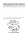
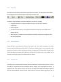
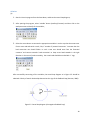
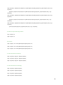
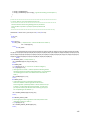
The conceptual links between these nine sectors are shown in Figure 1.1. The carbon sector computes
the atmospheric carbon dioxide concentration by considering the carbon exchange among ocean, air,
vegetation, humus and industrial emissions. The atmospheric temperature is produced by climate sector
taking into consideration the radiative forcing from different sources. The land-use sector deals with the
change of land-use by converting forest area to agricultural land and agricultural land to urban land to
meet the needs of growing population. Food production is driven by the availability of agricultural land,
allocated capital, water availability and land fertility. The requirements for the increase in food
production are driven by the population growth and per capita food demand. The population sector
computes the total population in each year for four different age groups (0 -14, 15-44, 45-65, 65 and
above) based on the desired number of children per family, birth control effectiveness, availability of
resources, and other factors. The energy-economy sector is formulated on the basis of market clearance
optimization. The energy-economy sector produces GDP, energy production and fossil fuel based
emissions. Hydrologic cycle is represented as surface water sector in the ANEMI model, which computes
precipitation, runoff, groundwater flow and other components of the hydrologic cycle. Water demand
sector calculates the demand for agricultural, domestic and industrial water uses. Water quality sector
deals with the physical and chemical characteristics of water based on the use and average pollution
load that is coming from each type of water use (domestic, industry, and agriculture).
Land Use
Emissions
Pollution
Index
Land Use
+
Clearing
and
Burning
+
Carbon
Atmospheric
+ +
CO2
Emission
Arable Land +
Index
Food
Industrial
Production
emission
+
+
Temperature
Per capita
Agricultural
food
allocation
Consumption
+
−
and Labour
Energy-Economy
Temperature
-
Water use
efficiency
Fertility
-
Climate
Water use Intensity
+
Population
-
+
GDP
per
capita
Water
Stress
+
−
+
Water Demand
+
Water
Consumption
+
Wastewater
Reuse
Wastewater
Treatment
+
Water Quality
−
Wastewater
Treatment and
Reuse
−
Water Hydrologic Cycle +
Stress
Temperatur
e
Figure 1.1: Major intersectoral links of ANEMI model
2
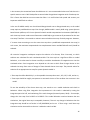
A detailed description of the inter-sectoral as well as intra-sectoral feedback relationships is available in
the main report (Akhtar et al, 2011). The ANEMI model is calibrated and verified against available
observations from 1980 to 2008 and information available in published literature. The model
performance is presented in the report to demonstrate the robustness of the ANEMI model as a climate
change policy analysis tool. The intension of this modeling effort is not the prediction of the future
system behaviour, but increased understanding of the complex interactions of society-biosphereclimate-economy-energy system
and response of different system sectors to various climate change
mitigation and adaptation policy options.
This manual should guide the users in operation of this system dynamics model for a range of land-use
conditions, water use policies, carbon tax implementation options and other policy alternatives. Two
versions of the ANEMI model are available: global and regional. The instructions in the manual apply to
both of them. The manual should help the users get familiar with:

Vensim;

MATLAB;

VisualStudio; and

Microsoft-Excel.
1.2 Organization of the Manual
This Manual is broadly divided in three parts. The first two chapters (Chapter 1 and Chapter 2) provide
basic information on the use of Vensim software (Ventana, 2010). Chapters 3 and 4 cover the mechanics
of building ANEMI model by integrating Vensim with other supporting software, and Chapter 5
demonstrates some advanced features of ANEMI model for policy implementation and analysis.
Chapter 1 provides an overview of this Manual. Chapter 2 introduces the user to the Vensim User
Interface and provides instructions for the installation of Vensim software. This chapter provides an
overview of Vensim’s functionalities, along with information on the Sketch tools, Analysis tools, and
Control windows. Chapter 3 provides a brief description of the ANEMI model, model experimentation
3
and policy description. Chapter 4 introduces other software packages required for the ANEMI model
simulation and their installation procedures. A detailed description of the integration procedure of
MATLAB and Vensim modeling tools through Visual Studio are also presented. Chapter 5 describes three
simulations which are related to different policy scenarios presented in the main report (Akhtar et al,
2011). This chapter also contains step-by-step procedure for the implementation of three policy
scenarios in both, global and regional versions of the ANEMI model. Appendix A contains the MATLAB
optimization code MATLAB for the energy-economy sector. This appendix contains programming code
for both, global and regional model, where ‘fsolve’ functionality is used to find a root (zero) of a system
of nonlinear equations. Appendix B includes all the necessary programming code in Visual Studio to
generate a Dynamic Link Library (*.DLL) files, which are utilized by Vensim; and Appendix D presents the
parameter estimation codes (in R programming language) developed for the disaggregation model.
4
2 VENSIM
Vensim (Ventana, 2010) is a visual system dynamics simulation modeling tool, which allows user to
conceptualize, document, simulate, analyze, and optimize models of dynamic systems. Vensim provides
a simple and flexible environment for building simulation model from the causal loop diagram, as well as
presenting it using stock and flow diagram. By connecting words with arrows, relationships among
system variables are entered and recorded as causal connections. The model can be analyzed
throughout the building process, looking at the causes and uses of a variable, and also looking at the
loops involving a variable. After completion of the model development, the model can be simulated and
user can thoroughly explore the behaviour of the model.
2.1 Vensim Basic Information
2.1.1
Directories
The typical installation path for Vensim is C:\Program Files\Vensim\models. However, the user can
install Vensim software at any location. When working with the model, it is strongly recommended that
the Vensim subdirectory be avoided (in this case C:\Program Files\Vensim).
2.1.2
Screen Shots
There is difference in the appearance of Vensim PLE, PLE Plus, Standard, Professional and DSS software
versions. All the pictures/screen views in this manual are extracted from the Vensim DSS and default
Toolsets (Ventana Systems, 2010).
2.1.3
Tab Dialog Boxes
Tab Dialogs are special dialog boxes common for Windows 95 and later versions of Windows. These
dialog boxes simplify controls by separating information into different "folders" with tabs. The user can
switch between folders by clicking on the appropriate tab.
5
2.1.4
Vensim Installation
To install Vensim, user needs to get the software, either from the CD or as a download from the
VENTANA Systems, Inc. website (http://www.vensim.com, last accessed, August 2011).
The Vensim CD
The Vensim CD contains the installation programs for all Vensim configurations. The label of the CD will
show the version number. Though installers for all configurations are included, the user will only be able
to install the specific configuration, as per the license agreement.
Downloading Vensim
The user is allowed to download Vensim from the website of VENTANA Systems inc. after the purchase
of Vensim license that includes one year of free electronic updates. The direct link for downloading
Vensim is http://www.vensim.com/cgibin/download.exe (last accessed, August 2011). This link is
available only with the valid registration code. The registration code identifies the productTo download
Vensim
PLE
(free
version
of
software)
for
educational purpose, user needs
to
visit
http://www.vensim.com/freedownload.html (last accessed, August 2011).
The Windows installer is broken into a number of relatively small files. The first of these files has a name
that depends on the product (for example, vendss32.exe for Vensim DSS). The remaining files are
labelled disk2.vip, disk3.vip and so on. When downloading, users must save all the files in the same
directory and it is very important that user should not change the name of any file.
2.1.5
Vensim Installation
Installation of the software can be done from the provided CD or downloaded files.
6
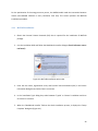
From CD
Insert the CD into the computer and follow the installation dialog. If there is any other previous version
of Vensim installed then the user may see the screen as shown in Figure 2.1. If this dialog does not open,
user needs to double click on the program file (setup.exe) on the installation CD.
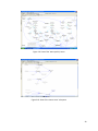
Figure 2.1: Initial Vensim installation screen
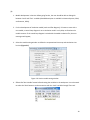
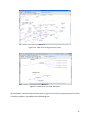
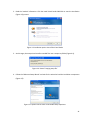
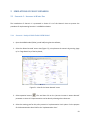
From the Installation Choices dialog, select the program that needs to be installed (Figure 2.2). The
installation starts by clicking on Install a Registered Vensim Application and entering the registration
code.
Figure 2.2: Installation choice dialog box
7
From Downloaded Files
Double click on the first file (for example, vendss32.exe for Vensim DSS). This will be in the directory
selected by the user during the download procedure.
2.1.6
Registration Code
Vensim DSS, Professional, Standard, PLE Plus and PLE for commercial use require a registration code.
Vensim PLE for educational or evaluation use do not require a registration code. Use of the ANEMI
model requires a licensed version of Vensim software, which allows work with the external
functionalities.
2.2 Main Features of Vensim Software
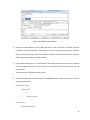
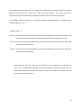
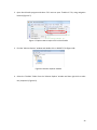
Vensim uses an interface workbench and a set of tools. The main Vensim window is the workbench,
which always includes the Title Bar, the Menu, the Toolbar, and the Analysis tools. When Vensim model
is open (Figure 2.3), the Sketch Tools and the Status Bar also appear.
Figure 2.3: View of the workbench window
The workbench variable is any variable in the model selected by the user. The workbench variable is
selected by clicking on a variable or by using the variable selection control in the control panel.
8
2.2.1
Vensim Menu
Many operations in Vensim can be performed from the menu.
 The File menu contains common functions such as Open, Save, Print, etc.
 The Edit menu allows the user to copy and paste selected portions of the model.
 The View menu has options for manipulating the sketch of the model and for viewing a model
as text-only (available only in Vensim Professional and DSS).
 The Layout menu allows user to manipulate the position and size of elements in the sketch.
 The Model menu provides access to the simulation control and the time bounds dialogs, the
model checking features, and importing and exporting datasets.

The Tools menu sets Vensim's global options and allows the user to manipulate analysis tools
and sketch tools as well as to set global options.
 The Windows menu enables the user to switch among different open windows.
 The Help menu provides access to the on-line help system.
Menus are context sensitive and the commands apply to whichever window currently is active. The
most commonly used menu commands also have shortcut keys and can be performed from the toolbar
described below.
2.2.2
Toolbar
The toolbar provides buttons for some of the most commonly used menu items and simulation features.
The first set of buttons access ‘File’ and ‘Edit’ menu items.
The next several buttons and the Runname editing box are used for model simulation.
9
The last few buttons access the window classes. User may need to click on a button to bring forward
that type of window or circulate through windows of that type.
2.2.3
The Build Window
Build window is used to create model in Vensim. By default, the window opens with the sketch tools for
sketching the structure of the model and for writing equations. The status bar provides buttons for
modifying the sketch. Each sketch view shows a part of the model, much like each page in a book tells
part of a story. In Vensim Professional and DSS, the build window can be switched to a text editor for
building and editing text-based models.
2.2.4
Sketch Tools
Sketch tools are grouped into a sketch toolset. Customized toolsets can be saved to files and reopened
for later use. The built in sketch toolset (default.sts) contains most of the sketch tools needed for
building models.
10
Vensim PLE and PLE Plus do not contain the Model Variable, Merge, Unhide Wand or Hide Wand tools.
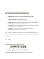
The sketch tools in the built in sketch toolset are:

Lock — sketch is locked. Pointer can select sketch objects and the Workbench Variable but
cannot move sketch objects.

Move/Size — move, sizes and selects sketch objects: variables, arrows, etc.

Variable — creates variables (Constants, Auxiliaries and Data).

Box Variable — create variables with a box shape (used for Levels or Stocks).

Arrow — creates straight or curved arrows.

Rate — creates Rate (or flow) construct, consisting of perpendicular arrows, a valve and, if
necessary, sources and sinks (clouds).

Model Variable — adds an existing model variable and the causes of that variable to the sketch
view.

Shadow Variable — adds an existing model variable to the sketch view as a shadow variable
(without adding its causes).

Merge — merges two variables into a single variable, merges Levels onto existing clouds,
merges Arrows onto a variable to split an Arrow, and performs other operations.

Input Output Object — adds input sliders and output graphs and tables to the sketch.

Sketch Comment — adds comments and pictures to the sketch.

Unhide Wand — unhide (makes visible) variables in a sketch view.

Hide Wand — hides variables in a sketch view.

Delete — deletes structure, variables in the model, and comments in a sketch.

Equations — create and edit model equations using the Equation Editor.
11
2.2.5
Status Bar
The status bar shows the state of the sketch and objects in the sketch. The status bar contains buttons
for changing the state of selected objects, and moving to another view.
A number of sketch attributes can be controlled from the status bar, including:

Change characteristics on selected variables; font type, size, bold, italic, underline,
strikethrough.

Set the hide level.

Variable colors, box color, surround shape, text position, arrow color, arrow width, arrow
polarity, and etc.

When using the ‘Text Editor’ (Vensim Professional and DSS), the Status Bar changes to reflect
text editing operations.
2.2.6
Output Windows
‘Output Windows, are generated by clicking on the ‘Analysis Tool’. The analysis tool gathers information
from the model and displays the information in a window as a diagram, graph, or text, depending on the
particular tool. Dozens of these windows can be open simultaneously, and a particular window can be
closed individually by clicking the Close button in the top left or top right corner, or all windows can be
closed at once using the menu item Windows>Close All Output.
2.2.7
Analysis Tool
The analysis tool is used to show information about the ‘Workbench’ variable, either its place or value in
the model, or its behaviour from the simulation datasets. Analysis tools are grouped into toolsets. To
configure a tool, user needs to click on the tool with the right mouse button and change its options.
Tools can also be added to a toolset. As with ‘Sketch’ toolsets, if the user makes changes he/she will be
12
prompted to save the toolset when exiting Vensim. Several different analysis toolsets are supplied with
Vensim, and can be opened from the menu Tools>Analysis Toolset>Open.
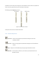
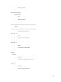
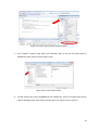
The following toolsets (Figure 2.4) are built-in.
Figure 2.4: Vensim built-in toolsets
A description of the functions of toolsets follows below.
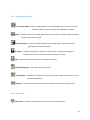
2.2.8
Structural Analysis Tools
Causes Tree — creates a tree-type graphical representation showing the causes of the
Workbench Variable.
Uses Tree — creates a tree-type graphical representation showing the uses of the Workbench
Variable.
Loops — displays a list of all feedback loops passing through the Workbench Variable.
Document — reviews equations, definitions, units of measure, and selected values for the
Workbench Variable.
13
2.2.9
Dataset Analysis Tools
Causes Strip Graph — displays simple graphs in a strip, allowing the user to trace causality by
showing the direct causes (as shown) of the Workbench Variable.
Graph — displays behaviour in a larger graph than the Strip Graph, and contains different options
for output than the Strip Graph.
Sensitivity Graph — creates a sensitivity graph of one variable and its range of uncertainty
generated from sensitivity testing.
Bar Graph — creates a bar graph of a variable at a specific time, or displays a histogram of
variables over all times or across sensitivity simulations at a time.
Table — generates a table of values for the Workbench Variable.
Table Running Down — table with time running down.
Runs Compare — compares all Lookups and Constants in the first loaded dataset to those in the
second loaded dataset.
Statistics — provides summary statistics on the Workbench Variable and its causes or uses.
2.2.10 Other Tools
Units Check — provides an alternative way to access the units check feature.
14
Equation Editor — provides an alternative way to access the equation for the Workbench
Variable.
Venapp Editor — supports the visual editing of Venapps.
Text Editor — a general purpose text editor.
Further details about model ‘views’ are available in the Vensim User’s Guide, version10 (Ventana
Systems, 2010), which is distributed with the software.
2.3 Numerical Integration Technique
The integration technique is the method that Vensim uses to advance a model in time. In software
package like Vensim DSS, actual computation of simulation requires numerical integration. Several
different types of numerical integration are available: Euler, Diff, Runge-Kutta4 auto, Runge-Kutta4
fixed, Runge-Kutta2 auto, and Runge-Kutta2 fixed techniques (Ventana Systems, 2010). Euler integration is
the simplest and fastest numerical method, but is less accurate than the Runge-Kutta method. Diff
performs Euler integration but stores the values for Auxiliaries computed at the previous save time.
Regular Euler integration stores the values of Auxiliaries computed at the current save time. Diff, as its
name suggests, is intended primarily for difference equations where this reporting convention is often
used. Runge-Kutta is modification of Euler integration that improves accuracy substantially by checking
derivatives between the set time-intervals, without imposing a heavy computational burden. Several
different Runge-Kutta intervals can be chosen in Vensim: fixed step size of one-half (fixed RK2) and onequarter (fixed RK4), as well as automatic adjustments of step size, (RK2 auto and RK4 auto). RK4 Auto
performs fourth order Runge-Kutta integration with automatic adjustment of the step size to ensure
accuracy. This is the best choice, if the user wants an accurate answer quickly, but requires significantly
more computational effort than the other forms. Therefore, RK4 auto is the slowest of the numerical
integration techniques. RK4 Fixed performs fourth order Runge-Kutta integration with a fixed step size
specified by TIME_STEP. This is usually very accurate, but does not detect own inaccuracies. RK2 Auto
which performs second order Runge-Kutta integration with automatic adjustment of the step size. This
15
is less accurate, but sometimes faster than RK4 auto. It is not recommended unless user feels there is a
special reason to use it. RK2 Fixed performs second order Runge-Kutta integration with a fixed step size.
This is faster than RK4 but more accurate than Euler. It is useful when both speed and accuracy are
important and difficult to achieve.
In the use of ANEMI model, user should avoid Runge-Kutta2 auto or Runge-Kutta4 auto, as the model
setup requires predefined time-step. Even though, ANEMI model is mostly build using system dynamic
based Vensim platform, still it has a dynamic link with outside computational environment (MATLAB). In
each time-step Vensim sends some information to MATLAB, to get a new set of parameters for the next
time step. Therefore it is essential to maintain same calculation time step for both programs. However,
if it seems time consuming to use the same time step then a predefined computational time step (in
such a case, the maximum computational time step between Vensim and MATLAB will work) should be
selected.
All numerical integration techniques require the selection of a discrete, finite ‘time-step’, at which
solutions are calculated for each simulated variable. This time step has a significant effect on model
behaviour, so its value must be chosen carefully to avoid the introduction of integration error into the
simulated values. Since integration error depends on the rate at which flows change relative to the
selected time step, faster rates of change in flows demand shorter time steps. The practical advice for
selection of an appropriate time step for system dynamics model is:
• Time steps should be divisible by 2, so that possible time step values are 1, 0.5, 0.25, 0.125, and so on;
• Time steps should be roughly one-quarter to one-tenth the size of the smallest time constant in the
model.
To test the suitability of the chosen time step, user needs to run a model simulation and check its
behaviour. When using Euler integration the improvement in the results is obtained by cutting the
integration period in half, and evaluationg if the result changes (Ventana Systems, 2010) – for example,
change the time step from 0.03125 to 0.015625. If the model behaviour matches between the two
simulations, the original time step is acceptable; however, if there is any change in behaviour then the
integration step should be cut further in half (0.0078128) and so on. If after using a small time step
simulation results mismatch then the user is advised to switch to RK4.
16
2.4 An Example
This section will illustrate how a system dynamics based simulation model can be developed with
Vensim software.
2.4.1
Problem Description and Solution
Problem:
Consider a small subdivision of London that is growing in population. Land available for housing
development is obtained by converting the agricultural land into urban. The total available agricultural
land is limited and can support the growth up to a certain level. With more potential home customers in
the subdivision, land conversion from the available agricultural land will increase. With more land
converted, the more actual home customers there will be. However, the higher land conversion brings
awareness that the available agricultural land is limited, and that inversely affects potential home
customers. The more land converted reduces the available agricultural land and makes less urban land
available for new homes.
Subdivision has 100 potential home customers; if the land for development is available 2.5% of potential
customers each month may decide to move to the subdivision and become actual customers (assume
that units for land conversion are expressed using number of customers – one customer is equal to one
home plot of land); total agricultural land available is sufficient for 85 customers.
The solution of the problem follows the procedure as outlined:
(a) Development of a causal diagram for the problem;
(b) Development of the corresponding stock and flow diagram;
(c) Development of the Vensim model for the problem;
(d) Simulation of the Vensim model.
17
Solution:
(a)
1. Start the Vensim program from the Start Menu, and draw the causal loop diagram;
2. After opening the program, select ‘variable’ button (Auxiliary/Constant) and then click on the
workspace area to identify all the variables;
3. Select the arrow button to connect the appropriate variables in such a way that the arrow starts
from a cause and ends with a result, like; if number of ‘potential customers’ increases then the
land conversion rate should follow. In such a case user should start from the ‘Potential
customer’ and connect towards ‘Land conversion’ to keep arrow head towards in the right
direction. In the case of positive causality, the arrow head should be marked with ‘+’ sign;
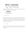
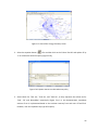
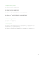
After successfully connecting all the variables, the causal-loop diagram as in Figure 2.5 should be
obtained. Polarity of causal relationships determines the sign of the feedback loop (Sterman, 2000).
-
Figure 2.5: Causal-loop diagram (the negative feedback loop)
18
(b)
1. Model development in Vensim. Before going further, the user should be able to distinguish
between ‘stock’ and ‘flow’ variables (detailed description is available in Ventana Systems, 2010;
and Sterman, 2000);
2. For the development of simulation model (stock and flow diagram), it’s better to start with a
new model, as casual loop diagram is not a simulation model. It only helps to formulate the
model structure. If the casual loop diagram is mixed with the model simulation file, the error
message could appear;
3. Select the model setting window to define the computational time step and simulation time
horizon (Figure 2.6)
Figure 2.6: Vensim model setting window
4. Select the ‘Box Variable’ button before drawing the variables in the workspace. User also needs
to select the ‘Rate’ button to make connection with the ‘stock’ variable through ‘flow rate’.
19
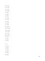
5. After the completion of all the required connections the stock and flow diagram of the model
should be like the diagram in Figure 2.7, where ‘Potential Customer’ and ‘Actual Customer’ are
stocks representing number of customers. ‘Land conversion’ is working as a flow by
transforming ‘Potential Customer’ to ‘Actual Customer’.
Figure 2.7: Stock and flow diagram
(c)
1. To incorporate the mathematical equations, the user needs to select the equation button before
clicking on any variable. After that, user will be able to edit the equation or incorporate equation
in the designated area (Figure 2.8).
20
Figure 2.8: Equation editor window
2. Define the initial conditions for the model two stocks. Insert ‘100’ and ‘0’ value for ‘Potential
Customer’ and ‘Actual Customer’ respectively. In this case at the beginning of the simulation
period, all of the customers (100) were potential customer as there was no home to handover,
which leads to zero number of actual customer.
3. In the problem description, it is mentioned that the project progress rate is aimed to transform
2.5% of potential customers to actual customer in each month. So the land conversion rate can
be defined as:
Land conversion = Potential customer*0.025
4. Vensim also allows user to visualize all the embedded equations under the diagram in the text
format, which looks as:
Actual customer= INTEG (
Land conversion,
0)
~
number of customer
~
|
Land conversion=
Potential customer*0.025
21
~
number of customer
~
|
Potential customer= INTEG (
-Land conversion,
100)
~
number of customer
~
|
********************************************************
.Control
********************************************************~
Simulation Control Parameters
FINAL TIME = 100
~
Month
~
The final time for the simulation.
|
INITIAL TIME = 0
~
Month
~
The initial time for the simulation.
|
SAVEPER =
TIME STEP
~
Month [0,?]
~
The frequency with which output is stored.
|
TIME STEP = 1
~
Month [0,?]
~
The time step for the simulation.
22
(d)
As the last step, model simulation is initiated by pressing ‘Run’ button from the Tool Bar. After
completion of the simulation, the user can visualize or extract the results file, both in graphical and
numerical format.
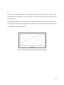
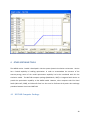
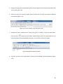
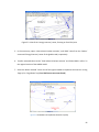
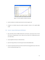
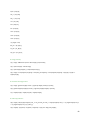
In the problem description, it is mentioned that the total land available is sufficient for 85 customers. So,
from the graph of actual customers (Figure 2.9), it can be seen that 75 months would be sufficient to sell
all the properties within the subdivision.
Figure 2.9: Time series plot of the number of actual customers
23
3
ANEMI MODEL
3.1 Model Organization and Mathematical Basis
The ANEMI version 2 model captures interconnections between main elements of the complex societybiosphere-climate-economy-energy system like global surface temperature, global CO2 concentration,
average annual surface flow, population growth, economic output, energy consumption, wastewater
volume, and others (Akhtar et al, 2011).
The system dynamics models include two levels of model representation: (i) a diagrammatic
representation of the causal connections that constitute the system under study, and (ii) the
mathematical basis of those connections in the form of equations.
Vensim allows the user to separate the model in many ways at the diagrammatic level. This unique
facility supports the ANEMI model structure – nine model sectors are developed using multiple system
dynamics diagrams. Conceptually, the sectoral view helps the user to focus on any specific sector by
drawing boundaries around the processes of importance in that part of the model. While looking at the
integrated modelling structure it is not uncommon that the majority of variables in one sector are not
relevant to the rest of the model, and their number within an individual sector is generally significantly
higher than the number of equations that connect different sectors. Finally, model division into
subsystems separates the relevant from the irrelevant variables, so that only key variables – those
involved in intersectoral feedbacks – are visible to the rest of the model.
The global version of ANEMI model is divided into fourteen subsystem views, which in most cases
correspond to model sectors. Those subsystems, which are not treated as sectors, are mainly introduced
to make the visual representation more tidy and convenient for the model user. These fourteen views of
nine ANEMI sectors are introduced in the Vensim DSS model version through the ‘view selector’ located
at the bottom of the main screen or by pressing the ‘page up’ and ‘page down’ key.
24
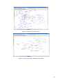
The model views are presented below in the following order (from Figure 3.1 through Figure 3.14):
carbon, other gasses, climate, climate_Nordhaus, land-use, food production, hydrologic cycle (water
quantity), water demand, water quality, water stress, population, emission, energy-economy, and sealevel rise.
Figure 3.1: View of the ‘carbon’ sector
Figure 3.2: View of the ‘other gasses’ subsystem
25
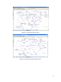
Figure 3.3: View of the ‘climate’ sector
Figure 3.4: View of the ‘climate_Nordhause’ subsystem
26
Figure 3.5: View of the ‘land-use’ sector
Figure 3.6: View of the ‘food production’ sector
27
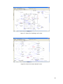
Figure 3.7: View of the ‘hydrologic cycle’ sector
Figure 3.8: View of the ‘water demand’ sector
28
Figure 3.9: View of the ‘water quality’ sector
Figure 3.10: View of the ‘water stress’ subsystem
29
Figure 3.11: View of the ‘population’ sector
Figure 3.12: View of the ‘emission’ subsystem
30
Figure 3.13 : View of the ‘energy-economy’ sector
Figure 3.14: View of the ‘sea-level’ subsystem
All the variables, constants and parameters shown in Figures 3.2 to 3.14 are representing stocks or flows
or auxiliary variables in the ANEMI stock and flow diagrams.
31
3.2 ANEMI Model Simulations
The ANEMI system dynamics modelling follows a structural approach of modelling, so that each
individual sector is based on the best understanding of the real-world. Here the structural approach
means that equations used to drive the model are not only based on a mathematical expressions and
matching data, but also on the current level of scientific understanding and judgment to appropriately
represent the physical processes occurring within the complex system. Therefore, it is often observed
that the ANEMI model fails to exhibit excellent match with the actual data.
At the same time, the
model is capable of avoiding data overfitting problem.
The greatest strength of the system dynamics model like ANEMI is its structure rather than the set of
equations that provides the best-fit to the data. So manipulation of the calibration parameters is not the
primary and only modeling objective. The calibration procedure concentrates primarily on the
manipulation of uncertain structural elements through alterations to stocks and flows and feedback
structures, whereas parameter tuning constitutes a minor part of the model calibration and verification
process.
The ANEMI version 2 model is tested following the three basic steps:
i)
Validation;
ii)
Checking the model behaviour by functional analysis; and
iii)
Checking the impact of feedback structure.
The ANEMI model is fully tested and above mentioned steps may be repeated only if the modifications
are made to the model structure. The main mode of model use by the user is through the
implementation of various policy options (‘what if’ scenarios) that can be created by changing /choosing
model input parameters. Implementation of the carbon tax scenario could be a good example for the
illustration of this process. The user could easily modify the parameter of carbon tax policy in this model
and track the consequences within few minutes after a successful model run. User needs not to be
restricted to simulation results within the energy-economy sector, but can analyze the behaviour of any
variable within the model structure including all model sectors.
32
3.3 Policy Development
The ANEMI model can be used to analyze the consequences of different policy scenarios. The policy
could be related to energy price, energy consumption, water use, water quality, irrigation practice,
population dynamics, land-use change and much more issues, which can be addressed by the analyses
of nine model sectors. ANEMI model structure allows for single or combined policy scenarios.
The following is description of policy development process and the implementation of a particular policy
with the ANEMI model.
3.3.1
Scenario 1 - Increase in Water Use
Key Question: What are the impacts from increase in water use?
The key question is converted into ‘what if’ scenario of maintaining current irrigation practices, and
whether such practices (and consequently agricultural output) can be sustained in case of increased
water stress. This scenario is examined with the global and regional version (focusing on Canada) of the
ANEMI model. As the food production sector is not only dependent on land-use, it is also possible to
assess the interaction between the food production and the changes in water population and variables
of the energy-economy sector. This scenario looks more broadly to several sectors including: hydrologic
cycle, water quality, energy-economy, population, climate, carbon, and food production. A 15% increase
in water use is considered under this scenario to meet future water demand.
In the ANEMI model the Scenario 1 is created by assigning the two input variables: ‘Water use increase
in %’, and ‘Implementation year’. In this case we decided to implement our scenario 1, from the year
2015. So the following modifications are required to implement the scenario 1 (Figures 3....and 3...):
‘Water use increase in %’ = 15
‘Implementation year’ = 2015
33
3.3.2
Scenario 2 – Increase in Food Production
Key Questions: What are the impacts from increased conversion rate of forest land into agricultural
land?
This scenario is closely related to the previous one. The scenario 2 tests the impact of changing the landuse by converting one land form into another – forest into agricultural land. In this scenario, 15%
increase in land conversion from forest to agricultural is implemented from the year 2015.
34
In the ANEMI model the Scenario 2 is created by assigning the following values to different input
variables: ‘Land transformation multiplying year’ stands for the increased land transformation start year,
and ‘Matrix Multiplier for Land Use Change’ denotes increase percent of deforestation for agricultural
use. Therefore the following modifications are required to implement the scenario 2 (Figures 3....and
3...):
‘Land transformation multiplying year’ =2015
‘Matrix Multiplier for Land Use Change’ = -0.15 in place of j1q1
here, j1q1 is the increased transfer rate of forest out of 1 (value in percent/100) and the sign determines
whether it’s in losing side or gaining side. In this case as the forest area is decreasing so j1q1 should be
negative.
Figure 3.15: Option view to choose land transformation rate
3.3.3
Scenario 3 - Carbon Tax
Key Questions: What are the impacts from implementing the carbon tax policy?
35
In the ANEMI energy-economy sector, the carbon tax is implemented as a tax per unit of CO 2 emissions,
effectively raising the price of fossil fuel. Under this experimentation, the carbon tax policy is
implemented in 2012 and then slowly ramped up to $100 per tonne of CO2 over next 30years.
In the ANEMI model the Scenario 3 is created by assigning the following values to different input
variables (Figures 3....to 3....) :
‘Carbon Tax ON’ =1;
‘Tau1 tax’= Starts from the year 2012 with an increment rate of 0.02218 until it reaches to 0.6654 in the
year 2041 and then continues with the same fixed value which is $100 per tonne of CO2.
‘Tau 2 tax’= Starts from the year 2012 with an increment rate of 0.01742 until it reaches to 0.5226 in the
year 2041 and then continues.
‘Tau3 tax’ = Starts from the year 2012 with an increment rate of 0.01246 until it reaches to 0.3739 in the
year 2041 and then continues.
Select values for ‘Tau1 tax’, ‘Tau2 tax’, and ‘Tau3 tax’, as they represent the carbon tax for
‘Coal’, ‘Oil’ and ‘NaturalGas’ respectively (In this demonstration, equivalent amount of tax is
implemented based on the emission intensity from each unit of fossil fuel. However, user can
implement any type of tax policy.
36
Look-up table for coal based carbon tax rate input
37
4
OTHER SOFTWARE TOOLS
The ANEMI version 2 model is developed in Vensim system dynamics simulation environment. Vensim
has a limited capability in handling optimization. In order to accommodate the structure of the
economy-energy sector of the model optimization capability had to be introduced with thin the
simulation model. The MATLAB computer package (MathWorks, 2007) is integrated with Vensim to
provide the optimization capability to the ANEMI model. However, other computer tools like Visual
Studio (Microsoft, 2008), and Microsoft Excel are also used to facilitate the dynamic data exchange
procedure between Vensim and MATLAB.
4.1 MATLAB Computer Package
38
For the optimization of the energy-economy sector, the ANEMI model needs the interaction between
Vensim and MATLAB software in every simulation time step. This section presents the MATLAB
installation procedure.
4.1.1
MATLAB Installation
1. Obtain the Personal License Password (PLP) that is required for the installation of MATLAB
package.
2. Use the installation DVD and follow the MathWorks Installer dialogue (Error! Reference source
not found.).
Figure 4.1: MATLAB installation option view
3. Enter the user name, organization name, and Personal License Password (PLP) in the license
information dialog box and select ‘Next’ to continue.
4. In the ‘Installation Type’ dialog box, select between ‘Typical’ or ‘Custom’ installation and then
click ‘Next’ to continue.
5. When the ’MathWorks Installer’ finishes the whole installation process, it displays the ‘Setup
Complete’ dialog box (Figure 4.2).
39
Figure 4.2: MATLAB setup completion message view
4.2 Visual Studio
The ANEMI model requires a number of functions that are not available in Vensim software. They can be
programmed externally using any programming language (usually C or C++) and then compiled into a
dynamic link library (DLL) which can be loaded by Vensim.
There are number of options for communication with Vensim, starting with the clipboard. Vensim can
also easily import or export data and constants from other sources. For dynamic control of Vensim's
behaviour, the Vensim DLL allows the user to control Vensim from Visual Basic, Delphi or any other
programming language. For the development of ANEMI model, the Visual studio package (Microsoft,
2008) is found to be the most suitable. For those ANEMI model users who will be modifying the model
structure familiarity with creation of DLL files to exchange data/information with Vensim is required.
4.2.1
Visual Studio Installation
1. As pre requirement, prior to the Visual Studio installation, system needs to be checked and
verified by the setup wizard. Execute Visual Studio installer.
40
2. Read the ‘readme’ information. Click the Install Visual Studio 2008 link to start the installation
(Figure 4.3) process.
Figure 4.3: Installation option view of the Visual Studio
3. At this stage, the setup wizard transfers needed files into a temporary folder (Figure 4.4);
Figure 4.4: View of ‘copying setup file’
4. Follow the ‘Welcome Setup Wizard’ and wait for the wizard to load the installation components
(Figure 4.5).
Figure 4.5: Option view to share Visual Studio setup experience
41
5.
Notice that, VS 2008 (version 8.x) needs .NET Framework version 3.5, where user needs to
provide the product key information and accept the license terms.
6. Proceed with the selection of installation choice between Default, Full or Custom.
7. Select the ‘Install’ button and follow the step-by-step auto installation process (Figure 4.6).
Figure 4.6: View of the installation process
4.3 Integration of External Functions With Vensim Software
A dynamic link library (DLL) is a collection of small programs, which can be called upon when needed by
the executable program (EXE) that is running. The DLL lets the executable use a particular functions.
Introduction of the optimization with the ANEMI model requires a few specialized functions such as:
reading from an external file, writing to an external file, and so on. Vensim DSS allows use of external
functions by Vensim software through a Dynamic Link Library (DLL). Such external functions can later be
used in Vensim, same as a built-in Vensim function.
4.3.1
Steps for DLL file compilation
1. Copy ‘TestDll’ folder from the supplied DVD (supplied with ANEMI model) and paste it in the
desired location.
42
2. Open Visual Studio program and select ‘File’ menu to open ‘TestDLL.sln’ file, using navigation
buttons (Figure 4.7).
Figure 4.7: Option view to import a file in Visual Studio
3. Find the ‘Solution Explorer’ window and double click on VENEXT.C file (Figure 4.8).
Figure 4.8: Solution explorer window
4. Select the ‘TestDLL1’ folder from the ‘Solution Explorer’ window and then right click to select
the ‘properties’ (Figure 4.9).
43
Figure 4.9: General options under solution explorer
5. From ‘TestDLL1’ Property Page, define the destination path of the DLL file (name could be
VENSIM.DLL) under ‘General’ option (Figure 4.10).
Figure 4.10: View of ‘Linker option’
6.
Provide required files name (VENSIMDP.LIB and VENEXT.DFF, which are shipped with Vensim
software package) under ‘Input’ option and then press ‘OK’ (Figure 4.11) to continue.
44
Figure 4.11: Definition file extraction window
7. Create the expected DLL file (VENSIM.DLL). Press ‘Debug’ button (
) and wait for the
result, which will appear in the ‘Output’ window (Figure 4.12).
Figure 4.12: Output window
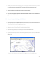
8. After successfully creating the DLL file, link that file (VENSIM.DLL) with Vensim. To do so, open
Vensim model and press ‘Option’ under the ‘Tools’ menu (Figure 4.13). ‘The global option
setting’ window will pop up and user needs to select ‘startup’ option before proceeding further
(Figure 4.14). Lastly, user should locate the DLL file (VENSIM.DLL), using the ‘Browse’ button
located beside the ‘External function Library’.
45
Figure 4.13: Option view of Vensim
Figure 4.14: Option view of ‘External function library’
9. Press ‘OK’ to complete the process.
4.3.2
Running Vensim and MATLAB Together
The whole ‘Model’ folder should be copied from the DVD supplied with the ANEMI model. As Vensim
and MATLAB are shearing some common files, it is suggested to carry out the simulation and
optimization work from the same folder. In the model folder supplied with the ANEMI model the user
will find all the required files (text files, Microsoft Excel files, Vensim files and MATLAB files).
Modification of these files is not allowed. The ANEMI model developers used a very specific way to set
up the simulation-optimization process, which requires exact procedure to be, followed (Figure 4.15):
46
Figure 4.15: Flow diagram of the file exchange process between Vensim and MATLAB
Global Version of the ANEMI Model
1. Open ‘out_back.txt’ file and save it as ‘out.txt’. This step needs to be carried out always at the
beginning of each simulation, as all the initial values for the optimization scheme are kept in the
‘out_back.txt’ file.
2.
Start MATLAB program first and then select ‘Open’ from the File menu (Figure 4.16).
Figure 4.16: View of the ‘File Menu’ in MATLAB
47
3. Navigate through newly created folder (where all files supplied on the DVD are kept) and select
‘ensect_solve_glb.m’ file.
4. Define the path to the working folder (where all files from the DVD are stored) in MATLAB
environment (Figure 4.17).
Figure 4.17: Place to define current directory path
5. Activate the ‘Editor’ window where, ‘ensect_solve_glb.m’ is loaded. To start the optimization,
press the ‘Run’ (
) button from the ‘Editor’ window (Figure 4.18). If the optimization for the
initial time step works, then MATLAB will create an ‘in.txt’ file for the Vensim model.
Figure 4.18: MATLAB ‘Editor’ window
6. Check the accuracy of the optimization by looking at the MATLAB ‘Command Window’ (Figure
4.19).
48
Figure 4.19: View of the MATLAB ‘Command Window’
7. Open the Vensim model from the ‘Start’ menu (Figure 4.20).
Figure 4.20: View of the ‘Start Vensim’
8. Select ‘Open Model’ from the ‘File’ menu. Choose ‘Global_model.mdl’ file (Figure 4.21).
49
Figure 4.21: File menu of Vensim
9. From the ‘Model’ menu select ‘Setting’ option, to setup the ‘Model Setting’ option (Figure 4.22).
This setup is required to define the simulation horizon as well as the computational time step
(Figure 4.23). Press ‘OK’ to proceed further.
Figure 4.22: Model setting option of Vensim
Figure 4.23: View of the ‘Time bound option’ under model setup option in Vensim
10. Check any specific parameter value or the model equation by using the equation button (
).
Select any parameter/variable/stock that maybe modified;
50
11. Before experimenting with the scenarios run a ‘base run’ to replicate the past and present
observations, without the implementation of any new policy.
12. Enter the name for the base model run - for example ‘Base’ (Figure 4.24).
Figure 4.24: Option view to define the name of the simulation output file
13. Press the ‘Run a Simulation’ button (
) to start the computation (Figure 4.25); and
Figure 4.25: View of the ‘Run a Simulation’ option
14. After successful completion of a model simulation, the results can be reviewed by selecting a
particulate variable from the ‘Dataset Analysis Tools’ menu bar (Figure 4.26). If the user wants
to see the graphical view of a variable then the ‘Graph’ button should be selected. In the same
way the numerical values can be obtained by selecting the ‘Table’ button.
Figure 4.26: View of the dataset analysis tools
51
Regional Version of the ANEMI Model
1. For the regional model, access ‘Regional’ folder before carrying out the start of simulation
process;
2.
Open ‘out_back.txt’ file and save it as ‘out.txt’.
3.
Start MATLAB program first and then select ‘Open’ from the ‘File’ menu;
4. Navigate through the newly created folder (where all files copied from the supplied DVD are
kept) and select ‘ensect_solve_can_apr17_1.m’ file.
5. Define the path to the working folder (where all files from the DVD are stored) in MATLAB
environment.
6. To start the optimization, press the ‘Run’ (
) button in the ‘Editor’ window of MATLAB. If the
optimization for the initial time step works fine then MATLAB will create an ‘in.txt’ file, which
will then be used by Vensim.
7. Open the Vensim model from the ‘start’ menu.
8. From the ‘File’ menu select ‘Open Model’ and select the ‘Regional Model.mdl’ file.
9. Select ‘Setting’ option from the ‘Model’ menu to setup the ‘Model Setting’ option. This setup is
required to define the simulation horizon and the computational time step.
10. Follow the same process from step 9 to step 14, presented for global version of the ANEMI
model to complete the simulation.
4.4 Important Remarks
52
If something goes wrong during the simulation process, user will not be able to stop the Vensim
software by only pressing ‘Escape’ key on the keyboard. As per the external function command, Vensim
is forced to wait until it gets a new text file (in.txt). In such a situation, press ‘Escape’ key first and then
open ‘b_in.txt’ file and save it as ‘in.txt’. Now, the decision can be made whether the result should be
saved or not. The user can also choose to continue the simulation but the chance of having erroneous
result is very high.
53
5 SIMULATIONS OF POLICY SCENARIOS
5.1 Scenario 1 – Increase in Water Use
The introduction of Scenario 1 is presented in Section 3.3.1 of this Manual. Here we present the
procedure for implementing Scenario 1 in ANEMI simulations.
5.1.1
Scenario 1 Analysis With Global ANEMI Model
1. Open the ANEMI model (Global_model.mdl) using Vensim software;
2. Select the ‘Water Demand’ sector view (Figure 5.1), to implement the scenario by pressing ‘page
up’ or ‘Page Down’ key of the key board;
Figure 5.1: View of the ‘water demand’ sector
3. Select equation button (
) first and then click on the ‘percent increase in water demand’
parameter to insert 15. Experimentation can be done by selecting other values too.
4. Select the starting year for this policy scenario in ‘Implementation Year’ option. For the purpose
of this demonstration select 2015 as the ‘Implementation Year’.
54
5. Save the model with a suitable name and close the Vensim program; and
6. Follow steps presented in Section 4.3.2 for running ANEMI global model to complete the
simulation of Scenario 1.
5.1.2
Scenario 1 Analysis With ANEMI Regional Model
Regional version of ANEMI is focused on Canada and the detailed description is in Akhtar et al, 2011.
Regional version of the ANEMI model has a close links with the rest of the world through climate, water,
and energy-economy sectors. Therefore, some of the simulation results obtained from the
implementation of global model are necessary for the simulation of the regional model.
1. Open the Global version of ANEMI model Scenario 1, to copy the ‘Price of fossil fuel’ from the
‘Energy-Economy’ sector. Select the ‘price of fossil fuel’ variable and then press on ‘Table’
button.
2. Export the content from the tabular view and ‘paste’ it in Microsoft Excel.
3. Open the ‘Energy-Economy’ view of the regional version of the ANEMI model (Regional
Model.mdl).
4. Import the respective fossil fuel price from the Excel file containing global fuel price for Coal, Oil,
and NaturalGas (Figure 5.2).
55
Figure 5.2: View of the ‘energy-economy’ sector, focusing on fossil fuel price
5. In the same way, export ‘new industrial carbon emission’, and ‘GDP1’ value from the ‘Carbon’
sector and ‘Energy-Economy’ sector of the global model, respectively.
6. Transfer extracted values as the ‘Total Industrial Carbon emission’ and ‘Global GDP in trillion’ in
the regional version of the ANEMI model.
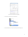
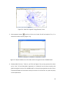
7. Select the ‘Water Demand’ sector view of the regional model to implement the Scenario 1 using
‘Page Up’ or ‘Page Down’ key (Error! Reference source not found.).
Figure 5.3: Parameters to implement Scenario 1 policy
56
7. Select equation button (
) first and then click on the ‘percent increase in water demand’ to
insert 15.
8. Choose the starting year for this policy implementation in the ‘Implementation Year’.
9. Save the model with a suitable name and close the Vensim program; and
10. Follow the procedures from Section 4.3.2 for simulating the regional ANEMI model.
5.2 Scenario 2 – Increase in Food Production
The introduction of Scenario 2 is presented in Section 3.3.2 of the Manual. In this section the
instructions are presented for simulating this scenario 2 with the ANEMI model.
5.2.1
Scenario 2 Analysis With Global ANEMI Model
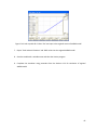
1. Select the ‘Land-Use’ view (Figure 5.4), to implement Scenario 2.
57
Figure 5.4: View of the ‘Land-Use’ sector
2. Select equation button (
) first and then click on the ‘Matrix Multiplier for Land use Change’.
3. Change the value of j1q1 to -0.15, which represents the additional land conversion from forest
to agricultural land by 15% (Figure 5.5).
Figure 5.5: Option view to choose land transformation rate
58
4. Modify ‘Land transformation multiplying year’. For the purpose of this demonstration year 2015
in ‘Land transformation multiplying year’ is selected as the policy implementation year.
5. Save the model with a suitable name and close the Vensim program.
6. Carry out the simulation following the procedure presented in Section 4.3.2 for simulating the
global version of ANEMI model.
5.2.2
Scenario 2 Analysis With Regional ANEMI Model
1. Open the Global version of ANEMI model which runs Scenario 2, to copy the simulated results of
‘Price of fossil fuel’ from the ‘Energy-Economy’ sector.
2. Export the values of ‘Price of fossil fuel’ variable to Microsoft Excel.
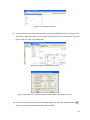
3. Open the ‘Energy-Economy’ view of the regional version of the ANEMI model.
4. Import the fossil fuel price from the Excel file with global fuel price for Coal, Oil, and NaturalGas
(Figure 5.6).
Figure 5.6: Fossil fuel price to be imported in the regional version of the ANEMI model
59
5. Export ‘New industrial Carbon Emission’, and ‘GDP1’ value from the ‘Carbon Sector’ and ‘EnergyEconomy’ sector of the global model, respectively.
6. Transfer exported values to ‘Total Industrial Carbon Emission’ and ‘Global GDP in trillion’ of the
regional version of the ANEMI model.
7. Open ‘Land-Use’ view (Figure 5.7), to implement the Scenario 2.
Figure 5.7: Parameters to implement with Scenario 2
8. Select equation button (
) first and then click on the ‘Matrix Multiplier for Land-Use Change’.
9. In the ‘Matrix multiplier for land use change’ change the value of ‘j1q1’ to -0.15, (Figure 5.8).
60
Figure 5.8: Option view to choose land use transformation rate (regional ANEMI model)
10. Change the ‘Land transformation multiplying year’.
11. Save the model with a suitable name and close the Vensim program.
12. Simulate Scenario 2 using procedure from the Section 4.3.2 for regional ANEMI model.
5.3 Scenario 3 - Carbon
The introduction of the carbon tax scenario is presented in Section 3.3.3 of this Manual. Here are the
instructions for the implementation of the carbon tax scenario with the ANEMI model.
5.3.1
Scenario 3 Analysis With Global ANEMI Model
1. Select the ‘Energy-Economy’ view (Figure 5.9), to implement the scenario;
61
Figure 5.9: View of the ‘Energy-Economy’ sector
2. Select the equation button (
) first and then click on the ‘Carbon Tax ON’ and replace ‘0’ by
‘1’ to activate the carbon tax policy (Figure 5.10);
Figure 5.10: Option view to turn ON carbon tax policy
3. Select values for ‘Tau1 tax’, ‘Tau2 tax’, and ‘Tau3 tax’, as they represent the carbon tax for
‘Coal’, ‘Oil’ and ‘NaturalGas’ respectively (Figure 5.11). In this demonstration, equivalent
amount of tax is implemented based on the emission intensity from each unit of fossil fuel.
However, user can implement any type of tax policy.
62
Figure 5.11: Look-up table for carbon tax rate input
4. Save the model with a suitable name and close the Vensim program; and
5. Complete the simulation using the procedure presented in Section 4.3.2 for global ANEMI
model.
5.3.2
Scenario 3 Analysis With Regional ANEMI Model
1. Open the Global version of ANEMI model which runs Scenario 3, and copy the ‘Price of Fossil
Fuel’ from the ‘Energy-Economy’ sector. Select the ‘Price of Fossil Fuel’ variable and then press
the ‘Table’ button;
2. Copy the global fossil fuel price in Microsoft Excel;
3. Open the ‘Energy-Economy’ view of the regional version of the ANEMI model;
4. Import the respective fossil fuel price from the Excel file containing global fuel price with tax for
Coal, Oil, and NaturalGas (Figure 5.12);
63
Figure 5.12: View of the regional ‘Energy-Economy’ sector
5. Select equation button (
) and then click on the ‘Carbon Tax ON’ and replace ‘0’ by ‘1’ to
activate the carbon tax policy (Figure 5.13);
Figure 5.13: Option window to turn ON carbon tax for the regional version of ANEMI model
6. Review/modify ‘Tau1 tax’, ‘Tau2 tax’, and ‘Tau3 tax’ (Figure 5.14), as they represent the carbon
tax for ‘Coal’, ‘Oil’ and ‘NaturalGas’ respectively. It is advised to use the same tax policy with
global and regional versions of the ANEMI model. In this experiment equivalent amount of tax is
implemented based on the emission intensity from each unit of fossil fuel. Any other tax policy
can be implemented.
64
Figure 5.14: Look-up table for ‘Carbon Tax’ rate input in the regional version of ANEMI model
7. Export ‘Total Industrial Emission’ and ‘GDP’ values into the regional ANEMI model.
8. Save the model with a suitable name and close the Vensim program.
9. Complete the simulation using procedure from the Section 4.3.2 for simulation of regional
ANEMI model.
65
REFERENCES
Akhtar, M. K., S. P. Simonovic, J. Wibe, J. MacGee, and J. Davies, (2011). An integrated system dynamics
model for analyzing behaviour of the social-energy-economic-climatic system: model description. Water
Resources Research Report no. 075 Facility for Intelligent Decision Support, Department of Civil and
Environmental Engineering, London, Ontario, Canada, 209 pages
Brink, A.B., and H.D. Eva, (2009). Monitoring 25 years of land cover change dynamics in Africa: a sample
based remote sensing approach. Applied Geography, 29: 501–512.
Davies, E. G. R. and S. P. Simonovic, (2008). An Integrated System Dynamics Model for Analyzing
Behaviour of the Social-Economic-Climatic System: Model Description and Model Use Guide. Facility for
Intelligent Decision Support, Department of Civil and Environmental Engineering, the University of
Western Ontario, London, Ontario, Canada.
Döll, P., (2002). Impact of climate change and variability on irrigation requirements: a global perspective.
Climatic Change, 54: 269–293.
Döll, P., M. Flörke, M. Mörker and S. Vassolo, (2003). Impact of climate change on water resources and
irrigation water requirements: a global analysis using new climate change scenarios. Klima–Wasser–
Flussgebietsmanagement – im Lichte der Flut, H.-B. Kleeberg, Ed., Proc. Tag der Hydrologie 2003 in
Freiburg, Germany, Forum für Hydrologie und Wasserbewirtschaftung, 11–14.
Downing, T.E, Butterfield, R.E., Edmonds, B., Knox, J.W., Moss, S., Piper, B.S. and Weatherhead, E.K. (and
the CCDeW project team) (2003). Climate Change and the Demand for Water, Research Report,
Stockholm Environment Institute Oxford Office, Oxford.
FAO (Food and Agricultural Organization), (2009). 2050: A Third More Mouths to Feed: Food Production
Will Have to Increase By 70 Percent – FAO Convenes High-Level Expert Forum. Available from
http://www.fao.org/news/story/0/item/35571/icode/en/, last accessed February 20, 2011.
Foley, J., de Fries, R., Defries, R., Asner, G.P., Barford, C., Bonan, G., Carpenter, S.R., Chapin, F.S., Coe,
M.T., Daily, G.C., Gibbs, H.K., Helkowski, J.H., Holloway, T., Howard, E., Kucharik, C.J., Monfreda, C., Patz,
J., Prentice, I.C., Ramankutty, N., Snyder, P.K., (2005). Global consequences of land use. Science, 309:
570–574.
Intergovernmental Panel on Climate Change (IPCC), (2007). Summary for Policymakers: Synthesis
Report. Paris.
IPCC Working Group II (2008). Climate Change and Water, Technical Paper VI, IPCC Working Group II
Technical Support Unit
Bates, B.C., Z.W. Kundzewicz, S. Wu and J.P. Palutikof, Eds., (2008). Climate Change and Water. Technical
Paper of the Intergovernmental Panel on Climate Change, IPCC Secretariat, Geneva, 210 pp.
66
Microsoft, (1998). Guide to Visual Studio 6.0(professional edition), Visual Studio: Developing for
Windows and the Web. Microsoft Corporation, USA.
Mote, P.W., D.J. Canning, D.L. Fluharty, R.C. Francis, J.F. Franklin, A.F. Hamlet, M. Hershman, M.
Holmberg, K.N. Gray-Ideker, W.S. Keeton, D.P. Lettenmaier, L.R. Leung, N.J. Mantua, E.L. Miles, B. Noble,
H. Parandvash, D.W. Peterson, A.K. Snover and S.R. Willard, (1999). Impacts of Climate Variability and
Change, Pacific Northwest, 110 pp. Available from
http://www.usgcrp.gov/usgcrp/Library/nationalassessment/pnw.pdf, last accessed Aug 10, 2011.
Neilsen, D., S. Smith, W. Koch, G. Frank, J. Hall, and P. Parchomchuk, (2001). Impact of Climate Change
on Crop Water Demand and Crop Suitability in the Okanagan Valley, BC. Technical Bulletin 01-15. Pacific
Agri-Food Research Centre, Summerland, British Columbia, Canada. Available from
http://adaptation.nrcan.gc.ca/projdb/pdf/4_e.pdf, last accessed Aug 15, 2011.
Protopapas, L., S. Katchamart and A. Platonova, (2000). Weather effects on daily water use in New York
City. J. Hydrol. Eng., 5: 332–338.
Schmidhuber, J., Tubiello, F.N., (2007). Global food security under climate change. Proceedings of the
National Academy of Sciences (USA), 104: 19703–19708.
Sterman, J. D. (2000). Business dynamics: Systems thinking and modeling for a complex world. The
McGraw-Hill Companies, Ltd., Boston, Massachusetts, U.S.A.
Ventana Systems. (2010). Vensim DSS Software (on line). Ventana Systems, Inc., Harvard,
Massachusetts, U.S.A. Available from http://www.vensim.com/documentation.html, last accessed
April.20, 2011.
MathWorks, (2007). MATLAB: getting started with MATLAB® 7 (on line), The MathWorks, Inc., MA.
Available from, http://www.mathworks.com/help/releases/R2007a/pdf_doc/matlab/getstart.pdf, last
accessed Dec 12, 2010.
67
APPENDIX A: ANEMI MODEL CODE (MATLAB)
Global ANEMI Model
List of Variables
Y
Total output
E
Aggregate energy services
Eh
Heat energy services
El
Electric energy services
Fh1
Coal used in heat energy production (GJ)
Fh2
Oil used in heat energy production (GJ)
Fh3
Natural gas used in heat energy production (GJ)
Fe1
Coal used in electricity production (GJ)
Fe2
Oil used in electricity production (GJ)
Fe3
Natural gas used in electricity production (GJ)
r
Gross interest rate
w
Wage rate
Pe
Price of aggregate energy services
Ph
Price of heat energy services
Pel
Price of electricity services
e4
electricity produced from nuclear power
e5
electricity produced from hydro power
FC1
Price of coal
FC2
Price of oil
FC3
Price of natural gas
TCe1
Total cost of electricity produced from coal
68
TCe2
Total cost of electricity produced from oil
TCe3
Total cost of electricity produced from natural gas
TCh1
Total cost of heat energy produced from coal
TCh2
Total cost of heat energy produced from oil
TCh3
Total cost of heat energy produced from natural gas
a1
CES weight for coal
a2
CES weight for oil
a3
CES weigth for natural gas
a1p
Short hand term for CES weight calculation for coal
a2p
Short hand term for CES weight calculation for oil
a3p
Short hand term for CES weight calculation for natural gas
Fh4
Alternative heat energy (GJ)
FC4
Price of alternatie heat energy
TCh4
Total cost of heat energy produced from alternative energy
short_El
Short hand term for electricity calculations
short_H
Short hand term for heat energy calculations
69
List of Parameters
gam1
Parameter for CES weight function for coal
gam2
Parameter for CES weight function for oil
gam3
Parameter for CES weight function for natural gas
b1
CES weight for coal
b2
CES weight for oil
b3
CES weight for natural gas
b4
CES weight for alternative heat energy
Pfz1
Base year price for coal
Pfz2
Base year price for oil
Pfz3
Base year price for natural gas
PR1
Current reserve value for coal
PR2
Current reserve value for oil
PR3
Current reserve value for natural gas
Rz1
Base year reserve value for coal
Rz2
Base year reserve value for oil
Rz3
Base year reserve value for natural gas
alpha
Capital's share
beta
Labour's share
gamma
Share parameter for energy aggregation
rho
Elasticity parameter for fossil fuel price function
theta
Elasticity parameter for energy aggregation
At
Total Factor Productivity
OMt
Nordhaus damage coefficient
L
Labour force
70
a4
Prescribed nuclear energy
a5
Prescribed hydro power
mu1
Parameter for alternative heat energy price function
mu2
Parameter for alternative heat energy price function
eta_e
Elasticity parameter for electricity production
eta_h
Elasticity paramater for heat energy production
om
Scale parameter for CES weights in electricity production
Ael
Electricity specific productivity term
Ah
Heat energy specific productivity term
tau1
Carbon tax rate for coal
tau2
Carbon tax rate for oil
tau3
Carbon tax rate for natural gas
nh_weight
CES weight for nuclear and hydro power
71
Solver File
This file is the primary ‘solver file’ used for the global ANEMI model. It takes inputs from Vensim, calls
the appropriate function, and produces the solution to the one-period energy-economy model.
clear all
tic
options1=optimset('FunValCheck','on', 'TolX',1.0e-9, 'TolFun',1.0e-9, 'MaxFunEvals',1.0e+9, ...
'MaxIter',0.100e+3, 'Display', 'iter', 'NonlEqnAlgorithm','dogleg');
options2=optimset('FunValCheck','on', 'TolX',1.0e-12, 'TolFun',1.0e-12, 'MaxFunEvals',1.0e+12, ...
'MaxIter',0.501e+3, 'Display', 'iter', 'NonlEqnAlgorithm','lm');
n=121;
time = linspace(1,n,121);
flag_vect = zeros(1,n);
par_check = zeros(37,n);
count2 = 1;
par_mat = xlsread('par_values_1.xls');
eng_mat = xlsread('eng_values.xls');
x0_cal = [2.91358474058133,2.06326283606995,1.62053847133827,4.11331109535488,0.301549557940114,0.194442342794547,-0.571260880029906,-2.17853176565763,-3.05841668528190,-3.90908781731049,1.85915914556616,1.48589400409797,-1.73994526093445,-1.62394359422644,-5.06755448357096,-3.71373791361643,2.71449037441833,-1.43801570954409,-0.533396790576313,-1.66283102760545,-2.04851166542617,-2.86752553959320,4.11858835525487,-1.73956526748421,-0.338954447781766,2.23409190763535,2.28985770205577,3.60298287203739,3.40364624800653,2.68549220816011,4.43877201412756,4.66470
844434739,-4.25209931331017,-2.31939186808372,-6.57149118139387,2.05665554767744,0.341023310827887,5.50885453934179,6.82192669034317,6.62260568833010,-1.58600226800754,-0.987779581613031,1.83169529110752];
cap = [35,0.655,0.188,0.080,0.352,0.823];
eng = eng_mat(1,:);
par = par_mat(1,:);
[xout_cal, fval, flag] = fsolve('energysect_glb_cal', x0_cal, options1, par, cap, eng);
if flag ~= 1
[xout_cal, fval, flag2] = fsolve('energysect_glb_cal', xout_cal, options2, par, cap, eng);
end
y = exp(xout_cal);
72
x0 = xout_cal(1,1:37);
x0_cal = xout_cal;
outmat(:,1) = y;
par_check(:,1) = par;
x0_zo = x0_cal(1,1:37);
par_ff = [y(1,9), y(1,28),y(1,31)];
par(1,1:6) = exp(x0_cal(1,38:43));
[xt_zo, fval, flag] = fsolve('energysect_glb_zo', x0_zo, options1, par, par_ff, cap);
if flag ~= 1
[xt_zo, fval, flag] = fsolve('energysect_glb_zo', x0_zo, options2, par, par_ff, cap);
end
x0_zo=xt_zo;
for i=1:n
filename ='out.txt';
mmfile = -1;
while(mmfile == -1)
pause(5);
mmfile = fopen(filename,'r');
end
par=fscanf(mmfile,'%e',[1 34]);
cap=fscanf(mmfile,'%e',[1 6]);
fclose(mmfile);
delete('out.txt');
eng = eng_mat(i,:);
par(1,35:37) = par(1,1:3);
if i<26
[xout_cal, fval, flag] = fsolve('energysect_glb_cal', x0_cal, options1, par, cap, eng);
if flag ~= 1
[xout_cal, fval, flag2] = fsolve('energysect_glb_cal', xout_cal, options2, par, cap, eng);
end
y = exp(xout_cal);
73
x0_cal=xout_cal;
x0 = x0_cal(1,1:37);
outmat(:,i) = y;
end
if i<26
par(1,1:6) = outmat(38:43,i);
else
par(1,1:6) = outmat(38:43,i-1).*(1 + 0.95*(outmat(38:43,i-1)-outmat(38:43,i-2))./outmat(38:43,i-2));
end
par_check(:,i) = par;
cap_check(:,i) = cap;
if count2 > 1 || exp(x0(1,9)) < 0.015
par_ff(1,1) = 0.015;
par_ff(1,2) = outmat(28,i-1);
par_ff(1,3) = outmat(31,i-1);
[xt, fval, flag] = fsolve('energysect_glb_zo', x0, options1, par, par_ff, cap);
if flag ~= 1
[xt, fval, flag] = fsolve('energysect_glb_zo', x0, options2, par, par_ff, cap);
end
x0=xt;
y=exp(xt);
outmat(1:37,i) = y;
outmat(38:43,i) = par(1,1:6);
count2 = count2+1;
else
x0_mat(:,i) = x0;
[xout, fval, flag] = fsolve('energysect_glb', x0, options1, par, cap);
if flag ~= 1
[xout, fval, flag] = fsolve('energysect_glb', xout, options2, par, cap);
end
74
y=exp(xout);
x0=xout;
x0 = x0_mat(:,i)';
par_ff = [y(1,9), y(1,28), y(1,31)];
[xt, fval, flag] = fsolve('energysect_glb_zo', x0, options1, par, par_ff, cap);
if flag ~= 1
[xt, fval, flag] = fsolve('energysect_glb_zo', xt, options2, par, par_ff, cap);
end
x0=xt;
yt=exp(xt);
outmat(1:37,i) = yt;
outmat(38:43,i) = par(1,1:6);
end
flag_vect(1,i) = flag;
fval_vect(1,i) = mean(abs(fval));
fval_mat(:,i) = fval;
y = outmat(1:37,i);
filename ='in.txt';
mmfile = fopen(filename,'w');
if ( mmfile == -1 )
disp(filename);
error('File not found');
end;
aa =fprintf(mmfile,'%e\n', y);
fclose(mmfile);
filename ='b_in.txt';
mmfile = fopen(filename,'w');
if ( mmfile == -1 )
disp(filename);
error('File not found');
75
end;
aa =fprintf(mmfile,'%e\n', y);
fclose(mmfile);
end
toc
76
Main Function File
The main function file for MATLAB solves the one-period problem for the global model. It is a non-linear
system of 37 equations and variables.
function z = energysect_glb(y,par,cap)
%variables
Y = y(1,1);
E = y(1,2);
Eh = y(1,3);
El = y(1,4);
Fh1 = y(1,5);
Fh2 = y(1,6);
Fh3 = y(1,7);
Fe1 = y(1,8);
Fe2 = y(1,9);
Fe3 = y(1,10);
r = y(1,11);
w = y(1,12);
Pe = y(1,13);
Ph = y(1,14);
Pel = y(1,15);
e4 = y(1,16);
e5 = y(1,17);
FC1 = y(1,18);
FC2 = y(1,19);
FC3 = y(1,20);
TCe1 = y(1,21);
TCe2 = y(1,22);
77
TCe3 = y(1,23);
TCh1 = y(1,24);
TCh2 = y(1,25);
TCh3 = y(1,26);
a1 = y(1,27);
a2 = y(1,28);
a3 = y(1,29);
a1p = y(1,30);
a2p = y(1,31);
a3p = y(1,32);
Fh4 = y(1,33);
FC4 = y(1,34);
TCh4 = y(1,35);
short_El = y(1,36);
short_H = y(1,37);
%capital
K = cap(1,1);
k1= cap(1,2);
k2= cap(1,3);
k3= cap(1,4);
k4= cap(1,5);
k5= cap(1,6);
%parameters
gam1 = par(1,1);
gam2 = par(1,2);
gam3 = par(1,3);
b1 = par(1,4);
78
b2 = par(1,5);
b3 = par(1,6);
Pfz1 = par(1,7);
Pfz2 = par(1,8);
Pfz3 = par(1,9);
PR1 = par(1,10);
PR2 = par(1,11);
PR3 = par(1,12);
Rz1 = par(1,13);
Rz2 = par(1,14);
Rz3 = par(1,15);
alpha = par(1,16);
beta = par(1,17);
gamma = par(1,18);
rho = par(1,19);
theta = par(1,20);
At = par(1,21);
OMt = par(1,22);
L = par(1,23);
a4 = par(1,24);
a5 = par(1,25);
b4 = par(1,26);
mu1 = par(1,27);
mu2 = par(1,28);
kap3 = par(1,29);
eta_e = par(1,30);
eta_h = par(1,31);
om = par(1,32);
Ael = par(1,33);
79
Ah = par(1,34);
tau1 = par(1,35);
tau2 = par(1,36);
tau3 = par(1,37);
nh_weight = 0.25;
% Energy economy
z(1) = exp(Y) - OMt*At*K.^alpha*L.^beta*exp(E).^(1-alpha-beta);
z(2) = alpha*L*exp(w) - beta*K*exp(r);
z(3) = alpha*exp(E)*exp(Pe) - (1-alpha-beta)*K*exp(r);
z(4) = exp(Y) + tau1*(exp(Fe1) + exp(Fh1)) + tau2*(exp(Fe2) + exp(Fh2)) + tau3*(exp(Fe3) + exp(Fh3)) - exp(r)*(K) - exp(w)*L exp(Pe)*exp(E);
% Aggregation of energy services
z(5) = exp(E) - (gamma*exp(Eh).^theta + (1-gamma)*exp(El).^theta).^(1./theta);
z(6) = gamma*exp(Pel)*exp(El)^(1-theta) - (1-gamma)*exp(Ph)*exp(Eh).^(1-theta);
z(7) = exp(Pe)*exp(E) - exp(Ph)*exp(Eh) - exp(Pel)*exp(El);
% Electricity production
z(8) = exp(El) - Ael*(exp(a1)*exp(Fe1).^eta_e + exp(a2)*exp(Fe2).^eta_e + exp(a3)*exp(Fe3).^eta_e +
nh_weight*exp(e4).^eta_e + nh_weight*exp(e5).^eta_e).^(1./eta_e);
z(9) = exp(Pel) - (exp(TCe1) + exp(TCe2) + exp(TCe3) + exp(r)*k4 + exp(r)*k5)./exp(El);
z(10) = ((exp(FC1) - (exp(FC1)-tau1)*exp(Fe1)*rho./(PR1-exp(Fe1)-exp(Fh1)))*(exp(short_El)./exp(a1p)) - exp(TCe1)) ...
- ((exp(FC2) - (exp(FC2)-tau2)*exp(Fe2)*rho./(PR2-exp(Fe2)-exp(Fh2)))*(exp(short_El)./exp(a2p)) - exp(TCe2));
z(11) = ((exp(FC2) - (exp(FC2)-tau2)*exp(Fe2)*rho./(PR2-exp(Fe2)-exp(Fh2)))*(exp(short_El)./exp(a2p)) - exp(TCe2)) ...
- ((exp(FC3) - (exp(FC3)-tau3)*exp(Fe3)*rho./(PR3-exp(Fe3)-exp(Fh3)))*(exp(short_El)./exp(a3p)) - exp(TCe3));
% Heat energy production
z(12) = exp(Eh) - Ah*(b1*exp(Fh1).^eta_h + b2*exp(Fh2).^eta_h + b3*exp(Fh3).^eta_h + b4*exp(Fh4).^eta_h).^(1./eta_h);
z(13) = exp(Ph) - (exp(TCh1) + exp(TCh2) + exp(TCh3) + exp(TCh4))./exp(Eh);
80
z(14) = ((exp(FC1) - (exp(FC1)-tau1)*exp(Fh1)*rho./(PR1-exp(Fe1)-exp(Fh1)))*(exp(short_H)./(b1*exp(Fh1).^(eta_h-1))) exp(TCh1)) ...
- ((exp(FC2) - (exp(FC2)-tau2)*exp(Fh2)*rho./(PR2-exp(Fe2)-exp(Fh2)))*(exp(short_H)./(b2*exp(Fh2).^(eta_h-1))) exp(TCh2));
z(15) = ((exp(FC2) - (exp(FC2)-tau2)*exp(Fh2)*rho./(PR2-exp(Fe2)-exp(Fh2)))*(exp(short_H)./(b2*exp(Fh2).^(eta_h-1))) exp(TCh2)) ...
- ((exp(FC3) - (exp(FC3)-tau3)*exp(Fh3)*rho./(PR3-exp(Fe3)-exp(Fh3)))*(exp(short_H)./(b3*exp(Fh3).^(eta_h-1))) exp(TCh3));
z(16) = ((exp(FC3) - (exp(FC3)-tau3)*exp(Fh3)*rho./(PR3-exp(Fe3)-exp(Fh3)))*(exp(short_H)./(b3*exp(Fh3).^(eta_h-1))) exp(TCh3)) ...
- ((1+mu2)*exp(FC4)*(exp(short_H)./(b4*exp(Fh4).^(eta_h-1))) - exp(TCh4));
% Nuclear and hydro electricity production
z(17) = exp(e4) - a4;
z(18) = exp(e5) - a5;
%Fuel prices
z(19) = exp(FC1) - tau1 - Pfz1*((PR1-exp(Fe1)-exp(Fh1))./Rz1).^rho;
z(20) = exp(FC2) - tau2 - Pfz2*((PR2-exp(Fe2)-exp(Fh2))./Rz2).^rho;
z(21) = exp(FC3) - tau3 - Pfz3*((PR3-exp(Fe3)-exp(Fh3))./Rz3).^rho;
% Total cost functions for electricity
z(22) = exp(TCe1) - exp(r)*k1 - exp(Fe1)*exp(FC1);
z(23) = exp(TCe2) - exp(r)*k2 - exp(Fe2)*exp(FC2);
z(24) = exp(TCe3) - exp(r)*k3 - exp(Fe3)*exp(FC3);
% Total cost functions for heat energy
z(25) = exp(TCh1) - exp(Fh1)*exp(FC1);
z(26) = exp(TCh2) - exp(Fh2)*exp(FC2);
z(27) = exp(TCh3) - exp(Fh3)*exp(FC3);
z(28) = exp(TCh4) - exp(Fh4)*exp(FC4);
81
% CES weights for electricity production
z(29) = exp(a1) - (1./om)*(gam1 - (exp(Fe1)./k1).^2);
z(30) = exp(a2) - (1./om)*(gam2 - (exp(Fe2)./k2).^2);
z(31) = exp(a3) - (1./om)*(gam3 - (exp(Fe3)./k3).^2);
z(32) = exp(Fe1).^(1-eta_e)*exp(a1p) - (exp(a1)*eta_e - (2./om)*(exp(Fe1)./k1).^2);
z(33) = exp(Fe2).^(1-eta_e)*exp(a2p) - (exp(a2)*eta_e - (2./om)*(exp(Fe2)./k2).^2);
z(34) = exp(Fe3).^(1-eta_e)*exp(a3p) - (exp(a3)*eta_e - (2./om)*(exp(Fe3)./k3).^2);
% Alternative Heat Energy Price Function
z(35) = exp(FC4) - mu1 - exp(Fh4).^mu2;
% Short-hand expressions
z(36) = exp(short_El) - (eta_e)*(exp(a1)*exp(Fe1).^eta_e + exp(a2)*exp(Fe2).^eta_e + exp(a3)*exp(Fe3).^eta_e +
nh_weight*exp(e4).^eta_e + nh_weight*exp(e5).^eta_e);
z(37) = exp(short_H) - (b1*exp(Fh1).^eta_h + b2*exp(Fh2).^eta_h + b3*exp(Fh3).^eta_h + b4*exp(Fh4).^eta_h);
82
Calibration Function File
The calibration function file for MATLAB solves the one-period problem for the global model, and
matches the historical trend for fossil fuel consumption in heat energy and electricity production.
function z = energysect_glb_cal(y,par,cap,eng)
%variables
Y = y(1,1);
E = y(1,2);
Eh = y(1,3);
El = y(1,4);
Fh1 = y(1,5);
Fh2 = y(1,6);
Fh3 = y(1,7);
Fe1 = y(1,8);
Fe2 = y(1,9);
Fe3 = y(1,10);
r = y(1,11);
w = y(1,12);
Pe = y(1,13);
Ph = y(1,14);
Pel = y(1,15);
e4 = y(1,16);
e5 = y(1,17);
FC1 = y(1,18);
FC2 = y(1,19);
FC3 = y(1,20);
TCe1 = y(1,21);
TCe2 = y(1,22);
83
TCe3 = y(1,23);
TCh1 = y(1,24);
TCh2 = y(1,25);
TCh3 = y(1,26);
a1 = y(1,27);
a2 = y(1,28);
a3 = y(1,29);
a1p = y(1,30);
a2p = y(1,31);
a3p = y(1,32);
Fh4 = y(1,33);
FC4 = y(1,34);
TCh4 = y(1,35);
short_El = y(1,36);
short_H = y(1,37);
gam1 = y(1,38);
gam2 = y(1,39);
gam3 = y(1,40);
b1 = y(1,41);
b2 = y(1,42);
b3 = y(1,43);
%capital
K = cap(1,1);
k1= cap(1,2);
k2= cap(1,3);
k3= cap(1,4);
k4= cap(1,5);
k5= cap(1,6);
84
%parameters
Pfz1 = par(1,7);
Pfz2 = par(1,8);
Pfz3 = par(1,9);
PR1 = par(1,10);
PR2 = par(1,11);
PR3 = par(1,12);
Rz1 = par(1,13);
Rz2 = par(1,14);
Rz3 = par(1,15);
alpha = par(1,16);
beta = par(1,17);
gamma = par(1,18);
rho = par(1,19);
theta = par(1,20);
At = par(1,21);
OMt = par(1,22);
L = par(1,23);
a4 = par(1,24);
a5 = par(1,25);
b4 = par(1,26);
mu1 = par(1,27);
mu2 = par(1,28);
kap3 = par(1,29);
eta_e = par(1,30);
eta_h = par(1,31);
om = par(1,32);
Ael = par(1,33);
Ah = par(1,34);
85
tau1 = par(1,35);
tau2 = par(1,36);
tau3 = par(1,37);
e1 = eng(1,1);
e2 = eng(1,2);
e3 = eng(1,3);
share_he1 = eng(1,4);
share_he2 = eng(1,5);
share_he3 = eng(1,6);
nh_weight = 0.25;
% Energy economy
z(1) = exp(Y) - OMt*At*K.^alpha*L.^beta*exp(E).^(1-alpha-beta);
z(2) = alpha*L*exp(w) - beta*K*exp(r);
z(3) = alpha*exp(E)*exp(Pe) - (1-alpha-beta)*K*exp(r);
z(4) = exp(Y) + tau1*(exp(Fe1) + exp(Fh1)) + tau2*(exp(Fe2) + exp(Fh2)) + tau3*(exp(Fe3) + exp(Fh3)) - exp(r)*(K) - exp(w)*L exp(Pe)*exp(E);
% Production of energy services
z(5) = exp(E) - (gamma*exp(Eh).^theta + (1-gamma)*exp(El).^theta).^(1./theta);
z(6) = gamma*exp(Pel)*exp(El)^(1-theta) - (1-gamma)*exp(Ph)*exp(Eh).^(1-theta);
z(7) = exp(Pe)*exp(E) - exp(Ph)*exp(Eh) - exp(Pel)*exp(El);
% Electricity production
z(8) = exp(El) - Ael*(exp(a1)*exp(Fe1).^eta_e + exp(a2)*exp(Fe2).^eta_e + exp(a3)*exp(Fe3).^eta_e +
nh_weight*exp(e4).^eta_e + nh_weight*exp(e5).^eta_e).^(1./eta_e);
z(9) = exp(Pel) - (exp(TCe1) + exp(TCe2) + exp(TCe3) + exp(r)*k4 + exp(r)*k5)./exp(El);
z(10) = ((exp(FC1) - (exp(FC1)-tau1)*exp(Fe1)*rho./(PR1-exp(Fe1)-exp(Fh1)))*(exp(short_El)./exp(a1p)) - exp(TCe1)) ...
- ((exp(FC2) - (exp(FC2)-tau2)*exp(Fe2)*rho./(PR2-exp(Fe2)-exp(Fh2)))*(exp(short_El)./exp(a2p)) - exp(TCe2));
z(11) = ((exp(FC2) - (exp(FC2)-tau2)*exp(Fe2)*rho./(PR2-exp(Fe2)-exp(Fh2)))*(exp(short_El)./exp(a2p)) - exp(TCe2)) ...
86
- ((exp(FC3) - (exp(FC3)-tau3)*exp(Fe3)*rho./(PR3-exp(Fe3)-exp(Fh3)))*(exp(short_El)./exp(a3p)) - exp(TCe3));
% Heat energy production
z(12) = exp(Eh) - Ah*(exp(b1)*exp(Fh1).^eta_h + exp(b2)*exp(Fh2).^eta_h + exp(b3)*exp(Fh3).^eta_h +
b4*exp(Fh4).^eta_h).^(1./eta_h);
z(13) = exp(Ph) - (exp(TCh1) + exp(TCh2) + exp(TCh3) + exp(TCh4))./exp(Eh);
z(14) = ((exp(FC1) - (exp(FC1)-tau1)*exp(Fh1)*rho./(PR1-exp(Fe1)-exp(Fh1)))*(exp(short_H)./(exp(b1)*exp(Fh1).^(eta_h-1))) exp(TCh1)) ...
- ((exp(FC2) - (exp(FC2)-tau2)*exp(Fh2)*rho./(PR2-exp(Fe2)-exp(Fh2)))*(exp(short_H)./(exp(b2)*exp(Fh2).^(eta_h-1))) exp(TCh2));
z(15) = ((exp(FC2) - (exp(FC2)-tau2)*exp(Fh2)*rho./(PR2-exp(Fe2)-exp(Fh2)))*(exp(short_H)./(exp(b2)*exp(Fh2).^(eta_h-1))) exp(TCh2)) ...
- ((exp(FC3) - (exp(FC3)-tau3)*exp(Fh3)*rho./(PR3-exp(Fe3)-exp(Fh3)))*(exp(short_H)./(exp(b3)*exp(Fh3).^(eta_h-1))) exp(TCh3));
z(16) = ((exp(FC3) - (exp(FC3)-tau3)*exp(Fh3)*rho./(PR3-exp(Fe3)-exp(Fh3)))*(exp(short_H)./(exp(b3)*exp(Fh3).^(eta_h-1))) exp(TCh3)) ...
- ((1+mu2)*exp(FC4)*(exp(short_H)./(b4*exp(Fh4).^(eta_h-1))) - exp(TCh4));
% Nuclear and hydro electricity production
z(17) = exp(e4) - a4;
z(18) = exp(e5) - a5;
%Fuel prices
z(19) = exp(FC1) - tau1 - Pfz1*((PR1-exp(Fe1)-exp(Fh1))./Rz1).^rho;
z(20) = exp(FC2) - tau2 - Pfz2*((PR2-exp(Fe2)-exp(Fh2))./Rz2).^rho;
z(21) = exp(FC3) - tau3 - Pfz3*((PR3-exp(Fe3)-exp(Fh3))./Rz3).^rho;
% Total cost functions for electricity
z(22) = exp(TCe1) - exp(r)*k1 - exp(Fe1)*exp(FC1);
z(23) = exp(TCe2) - exp(r)*k2 - exp(Fe2)*exp(FC2);
z(24) = exp(TCe3) - exp(r)*k3 - exp(Fe3)*exp(FC3);
87
% Total cost functions for heat energy
z(25) = exp(TCh1) - exp(Fh1)*exp(FC1);
z(26) = exp(TCh2) - exp(Fh2)*exp(FC2);
z(27) = exp(TCh3) - exp(Fh3)*exp(FC3);
z(28) = exp(TCh4) - exp(Fh4)*exp(FC4);
% CES weights for electricity production
z(29) = exp(a1) - (1./om)*(exp(gam1) - (exp(Fe1)./k1).^2);
z(30) = exp(a2) - (1./om)*(exp(gam2) - (exp(Fe2)./k2).^2);
z(31) = exp(a3) - (1./om)*(exp(gam3) - (exp(Fe3)./k3).^2);
z(32) = exp(Fe1).^(1-eta_e)*exp(a1p) - (exp(a1)*eta_e - (2./om)*(exp(Fe1)./k1).^2);
z(33) = exp(Fe2).^(1-eta_e)*exp(a2p) - (exp(a2)*eta_e - (2./om)*(exp(Fe2)./k2).^2);
z(34) = exp(Fe3).^(1-eta_e)*exp(a3p) - (exp(a3)*eta_e - (2./om)*(exp(Fe3)./k3).^2);
% Alternative Heat Energy Price Function
z(35) = exp(FC4) - mu1 - exp(Fh4).^mu2;
% Short-Hand Expressions
z(36) = exp(short_El) - (eta_e)*(exp(a1)*exp(Fe1).^eta_e + exp(a2)*exp(Fe2).^eta_e + exp(a3)*exp(Fe3).^eta_e +
nh_weight*exp(e4).^eta_e + nh_weight*exp(e5).^eta_e);
z(37) = exp(short_H) - (exp(b1)*exp(Fh1).^eta_h + exp(b2)*exp(Fh2).^eta_h + exp(b3)*exp(Fh3).^eta_h + b4*exp(Fh4).^eta_h);
% Matching Trend in Fossil Fuels
z(38) = exp(Fe1) - e1;
z(39) = exp(Fe2) - e2;
z(40) = exp(Fe3) - e3;
z(41) = exp(Fh1)./exp(Fe1) - share_he1;
z(42) = exp(Fh2)./exp(Fe2) - share_he2;
z(43) = exp(Fh3)./exp(Fe3) - share_he3;
88
Zero-Oil Condition Function File
The zero-oil function file for MATLAB solves the one-period problem for the global model when a cut-off
condition is satisfied. In response to price changes for a fossil fuel type, production of electricity can fall
much faster than the depreciation of the capital stock used in production of electricity from that fuel
type. As a result, the average total cost may increase very rapidly, and the non-linear equation solver
can break down. This event almost always happens to electricity production from oil, and the zero-oil
MATLAB function is a fix for that specific problem. When a threshold condition is reached, the value of
electricity produced from oil remains fixed at a level close to zero.
function z = energysect_glb_zo(y,par, par_ff,cap)
%variables
Y = y(1,1);
E = y(1,2);
Eh = y(1,3);
El = y(1,4);
Fh1 = y(1,5);
Fh2 = y(1,6);
Fh3 = y(1,7);
Fe1 = y(1,8);
Fe2 = y(1,9);
Fe3 = y(1,10);
r = y(1,11);
w = y(1,12);
Pe = y(1,13);
Ph = y(1,14);
Pel = y(1,15);
e4 = y(1,16);
e5 = y(1,17);
FC1 = y(1,18);
89
FC2 = y(1,19);
FC3 = y(1,20);
TCe1 = y(1,21);
TCe2 = y(1,22);
TCe3 = y(1,23);
TCh1 = y(1,24);
TCh2 = y(1,25);
TCh3 = y(1,26);
a1 = y(1,27);
a2 = y(1,28);
a3 = y(1,29);
a1p = y(1,30);
a2p = y(1,31);
a3p = y(1,32);
Fh4 = y(1,33);
FC4 = y(1,34);
TCh4 = y(1,35);
short_El = y(1,36);
short_H = y(1,37);
%capital
K = cap(1,1);
k1= cap(1,2);
k2= cap(1,3);
k3= cap(1,4);
k4= cap(1,5);
k5= cap(1,6);
90
%parameters
gam1 = par(1,1);
gam2 = par(1,2);
gam3 = par(1,3);
b1 = par(1,4);
b2 = par(1,5);
b3 = par(1,6);
Pfz1 = par(1,7);
Pfz2 = par(1,8);
Pfz3 = par(1,9);
PR1 = par(1,10);
PR2 = par(1,11);
PR3 = par(1,12);
Rz1 = par(1,13);
Rz2 = par(1,14);
Rz3 = par(1,15);
alpha = par(1,16);
beta = par(1,17);
gamma = par(1,18);
rho = par(1,19);
theta = par(1,20);
At = par(1,21);
OMt = par(1,22);
L = par(1,23);
a4 = par(1,24);
a5 = par(1,25);
b4 = par(1,26);
mu1 = par(1,27);
mu2 = par(1,28);
91
kap3 = par(1,29);
eta_e = par(1,30);
eta_h = par(1,31);
om = par(1,32);
Ael = par(1,33);
Ah = par(1,34);
tau1 = par(1,35);
tau2 = par(1,36);
tau3 = par(1,37);
nh_weight = 0.25;
fe2_par = par_ff(1,1);
a2_par = par_ff(1,2);
a2p_par = par_ff(1,3);
% Energy economy
z(1) = exp(Y) - OMt*At*K.^alpha*L.^beta*exp(E).^(1-alpha-beta);
z(2) = alpha*L*exp(w) - beta*K*exp(r);
z(3) = alpha*exp(E)*exp(Pe) - (1-alpha-beta)*K*exp(r);
z(4) = exp(Y) + tau1*(exp(Fe1)+exp(Fh1)) + tau2*(fe2_par+exp(Fh2)) + tau3*(exp(Fe3)+exp(Fh3)) - exp(r)*(K) - exp(w)*L exp(Pe)*exp(E);
% Production of energy services
z(5) = exp(E) - (gamma*exp(Eh).^theta + (1-gamma)*exp(El).^theta).^(1./theta);
z(6) = gamma*exp(Pel)*exp(El)^(1-theta) - (1-gamma)*exp(Ph)*exp(Eh).^(1-theta);
z(7) = exp(Pe)*exp(E) - exp(Ph)*exp(Eh) - exp(Pel)*exp(El);
% Electricity production
z(8) = exp(El) - Ael*(exp(a1)*exp(Fe1).^eta_e + a2_par*fe2_par.^eta_e + exp(a3)*exp(Fe3).^eta_e + nh_weight*exp(e4).^eta_e
+ nh_weight*exp(e5).^eta_e).^(1./eta_e);
z(9) = exp(Pel) - (exp(TCe1) + exp(TCe2) + exp(TCe3) + exp(r)*k4 + exp(r)*k5)./exp(El);
92
z(10) = ((exp(FC1) - (exp(FC1)-tau1)*exp(Fe1)*rho./(PR1-exp(Fe1)-exp(Fh1)))*(exp(short_El)./exp(a1p)) - exp(TCe1)) ...
- ((exp(FC2) - (exp(FC2)-tau2)*fe2_par*rho./(PR2-fe2_par-exp(Fh2)))*(exp(short_El)./a2p_par) - exp(TCe2));
z(11) = ((exp(FC2) - (exp(FC2)-tau2)*fe2_par*rho./(PR2-fe2_par-exp(Fh2)))*(exp(short_El)./a2p_par) - exp(TCe2)) ...
- ((exp(FC3) - (exp(FC3)-tau3)*exp(Fe3)*rho./(PR3-exp(Fe3)-exp(Fh3)))*(exp(short_El)./exp(a3p)) - exp(TCe3));
% Heat energy production
z(12) = exp(Eh) - Ah*(b1*exp(Fh1).^eta_h + b2*exp(Fh2).^eta_h + b3*exp(Fh3).^eta_h + b4*exp(Fh4).^eta_h).^(1./eta_h);
z(13) = exp(Ph) - (exp(TCh1) + exp(TCh2) + exp(TCh3) + exp(TCh4))./exp(Eh);
z(14) = ((exp(FC1) - (exp(FC1)-tau1)*exp(Fh1)*rho./(PR1-exp(Fe1)-exp(Fh1)))*(exp(short_H)./(b1*exp(Fh1).^(eta_h-1))) exp(TCh1)) ...
- ((exp(FC2) - (exp(FC2)-tau2)*exp(Fh2)*rho./(PR2-fe2_par-exp(Fh2)))*(exp(short_H)./(b2*exp(Fh2).^(eta_h-1))) exp(TCh2));
z(15) = ((exp(FC2) - (exp(FC2)-tau2)*exp(Fh2)*rho./(PR2-fe2_par-exp(Fh2)))*(exp(short_H)./(b2*exp(Fh2).^(eta_h-1))) exp(TCh2)) ...
- ((exp(FC3) - (exp(FC3)-tau3)*exp(Fh3)*rho./(PR3-exp(Fe3)-exp(Fh3)))*(exp(short_H)./(b3*exp(Fh3).^(eta_h-1))) exp(TCh3));
z(16) = ((exp(FC3) - (exp(FC3)-tau3)*exp(Fh3)*rho./(PR3-exp(Fe3)-exp(Fh3)))*(exp(short_H)./(b3*exp(Fh3).^(eta_h-1))) exp(TCh3)) ...
- ((1+mu2)*exp(FC4)*(exp(short_H)./(b4*exp(Fh4).^(eta_h-1))) - exp(TCh4));
% Nuclear and hydro electricity production
z(17) = exp(e4) - a4;
z(18) = exp(e5) - a5;
%Fuel prices
z(19) = exp(FC1) - tau1 - Pfz1*((PR1-exp(Fe1)-exp(Fh1))./Rz1).^rho;
z(20) = exp(FC2) - tau2 - Pfz2*((PR2-fe2_par-exp(Fh2))./Rz2).^rho;
z(21) = exp(FC3) - tau3 - Pfz3*((PR3-exp(Fe3)-exp(Fh3))./Rz3).^rho;
% Total cost functions for electricity
z(22) = exp(TCe1) - exp(r)*k1 - exp(Fe1)*exp(FC1);
93
z(23) = exp(TCe2) - exp(r)*k2 - fe2_par*exp(FC2);
z(24) = exp(TCe3) - exp(r)*k3 - exp(Fe3)*exp(FC3);
% Total cost functions for heat energy
z(25) = exp(TCh1) - exp(Fh1)*exp(FC1);
z(26) = exp(TCh2) - exp(Fh2)*exp(FC2);
z(27) = exp(TCh3) - exp(Fh3)*exp(FC3);
z(28) = exp(TCh4) - exp(Fh4)*exp(FC4);
% CES weights for electricity production
z(29) = exp(a1) - (1./om)*(gam1 - (exp(Fe1)./k1).^2);
z(30) = a2_par - exp(a2);
z(31) = exp(a3) - (1./om)*(gam3 - (exp(Fe3)./k3).^2);
z(32) = exp(Fe1).^(1-eta_e)*exp(a1p) - (exp(a1)*eta_e - (2./om)*(exp(Fe1)./k1).^2);
z(33) = a2p_par - exp(a2p);
z(34) = exp(Fe3).^(1-eta_e)*exp(a3p) - (exp(a3)*eta_e - (2./om)*(exp(Fe3)./(k3)).^2);
% Alternative Heat Energy Price Function
z(35) = exp(FC4) - mu1 - exp(Fh4).^mu2;
% Short-Hand Expressions
z(36) = exp(short_El) - (eta_e)*(exp(a1)*exp(Fe1).^eta_e + a2_par*fe2_par.^eta_e + exp(a3)*exp(Fe3).^eta_e +
nh_weight*exp(e4).^eta_e + nh_weight*exp(e5).^eta_e);
z(37) = exp(short_H) - (b1*exp(Fh1).^eta_h + b2*exp(Fh2).^eta_h + b3*exp(Fh3).^eta_h + b4*exp(Fh4).^eta_h);
z(38) = exp(Fe2) - fe2_par;
94
Regional ANEMI Model
List of Variables
Y
Total output
E
Aggregate energy services
Eh
Heat energy services
El
Electric energy services
Fh1
Coal used in heat energy production (GJ)
Fh2
Oil used in heat energy production (GJ)
Fh3
Natural gas used in heat energy production (GJ)
Fe1
Coal used in electricity production (GJ)
Fe2
Oil used in electricity production (GJ)
Fe3
Natural gas used in electricity production (GJ)
r
Gross interest rate
w
Wage rate
Pe
Price of aggregate energy services
Ph
Price of heat energy services
Pel
Price of electricity services
e4
electricity produced from nuclear power
e5
electricity produced from hydro power
FC1
Price of coal
FC2
Price of oil
FC3
Price of natural gas
TCe1
Total cost of electricity produced from coal
TCe2
Total cost of electricity produced from oil
95
TCe3
Total cost of electricity produced from natural gas
TCh1
Total cost of heat energy produced from coal
TCh2
Total cost of heat energy produced from oil
TCh3
Total cost of heat energy produced from natural gas
a1
CES weight for coal
a2
CES weight for oil
a3
CES weigth for natural gas
a1p
Short hand term for CES weight calculation for coal
a2p
Short hand term for CES weight calculation for oil
a3p
Short hand term for CES weight calculation for natural gas
Fh4
Alternative heat energy (GJ)
FC4
Price of alternatie heat energy
TCh4
Total cost of heat energy produced from alternative energy
short_El
Short hand term for electricity calculations
short_H
Short hand term for heat energy calculations
imports
Net Imports of the generic consumption good
96
List of Parameters
gam1
Parameter for CES weight function for coal
gam2
Parameter for CES weight function for oil
gam3
Parameter for CES weight function for natural gas
b1
CES weight for coal
b2
CES weight for oil
b3
CES weight for natural gas
b4
CES weight for alternative heat energy
Pfz1
Base year price for coal
Pfz2
Base year price for oil
Pfz3
Base year price for natural gas
PR1
Current reserve value for coal
PR2
Current reserve value for oil
PR3
Current reserve value for natural gas
Rz1
Base year reserve value for coal
Rz2
Base year reserve value for oil
Rz3
Base year reserve value for natural gas
alpha
Capital's share
beta
Labour's share
gamma
Share parameter for energy aggregation
rho
Elasticity parameter for fossil fuel price function
theta
Elasticity parameter for energy aggregation
At
Total Factor Productivity
OMt
Nordhaus damage coefficient
L
Labour force
97
a4
Prescribed nuclear energy
a5
Prescribed hydro power
mu1
Parameter for alternative heat energy price function
mu2
Parameter for alternative heat energy price function
eta_e
Elasticity parameter for electricity production
eta_h
Elasticity paramater for heat energy production
om
Scale parameter for CES weights in electricity production
Ael
Electricity specific productivity term
Ah
Heat energy specific productivity term
tau1
Carbon tax rate for coal
tau2
Carbon tax rate for oil
tau3
Carbon tax rate for natural gas
nh_weight
CES weight for nuclear and hydro power
fstar1
Total extraction of coal
fstar2
Total extraction of oil
fstar3
Total extraction of natural gas
98
Solver File
This file is the primary ‘solver file’ used for the regional model. It takes inputs from Vensim, calls the
appropriate function, and produces the solution to the one-period energy-economy model.
clear all
tic
options1=optimset('FunValCheck','on', 'TolX',1.0e-9, 'TolFun',1.0e-9, 'MaxFunEvals',1.0e+9, ...
'MaxIter',0.051e+3, 'Display', 'iter', 'NonlEqnAlgorithm','dogleg');
options2=optimset('FunValCheck','on', 'TolX',1.0e-12, 'TolFun',1.0e-12, 'MaxFunEvals',1.0e+9, ...
'MaxIter',1.011e+3, 'Display', 'iter', 'NonlEqnAlgorithm','lm');
x0_cal = [4.08882001940707,-0.477802471321497,1.38426580086723,2.43003911005965,0.230743656881343,1.06679573151687,0.279711343878389,-1.45433621280950,3.38146807797842,-4.12182604247513,-0.347451630119205,1.14350553864074,1.97635532528274,2.32422647439778,1.78015055840188,-1.83328793692455,-0.0684980216000813,2.59497758980671,0.0611390618024763,2.22719517990958,1.56773148361856,-3.13516025436419,-4.20981366794375,-1.20727187582513,0.533398961718562,1.38311945574640,0.698809043866189,2.07385907461717,1.53313088975904,0.635842215996799,3.05030256250949,2.867
66011154329,-3.14436512203694,1.95809178328180,-1.18627333875515,0.521872374469884,0.692132900433612,1.07418779215341,3.94053013691443,5.29795162282076,4.76014608768349,-2.68363371516625,1.90339098334132,-2.85895371745158];
par_mat = xlsread('par_values_can_2.xls');
cap_mat = xlsread('cap_values_can_3.xls');
eng_mat = xlsread('eng_values_can.xls');
cap = cap_mat(1,:);
eng = eng_mat(1,:);
par = par_mat(1,:);
n=121;
time = linspace(1,n,121);
flag_vect = zeros(1,n);
x0_v = ones(1,3);
par(1,10:12) = par(1,10:12);
99
vdg = fsolve('vedge', x0_v, options2, par, eng);
par(1,41:43) = par(1,10:12) - vdg.*par(1,13:15).*(par(1,38:40)./par(1,7:9)).^(1./par(1,19))
[xout_cal, fval, flag] = fsolve('energysect_cal_can', x0_cal, options1, par, cap, eng);
if flag ~= 1
[xout_cal, fval, flag2] = fsolve('energysect_cal_can', xout_cal, options2, par, cap, eng);
end
for j=1:3
if par(1,40+j) < 0
par(1,40+j) = 0;
end
end
y = exp(xout_cal);
y(1,18:20) = log(y(1,18:20));
y(1,38) = log(y(1,38));
x0 = xout_cal(1,1:38);
x0_cal = xout_cal;
outmat(:,1) = y;
x0_cal_int = x0_cal;
for i=1:n
filename ='out.txt';
mmfile = -1;
while(mmfile == -1)
pause(5);
mmfile = fopen(filename,'r');
end
par(1,1:34)=fscanf(mmfile,'%e',[1 34]);
par(1,35:40)=par(1,1:6);
cap=fscanf(mmfile,'%e',[1 6]);
fclose(mmfile);
delete('out.txt');
if i==1
100
eng = eng_mat(1,:);
res_mat(1,:) = par(1,10:12);
vdg = fsolve('vedge', x0_v, options2, par, eng);
par(1,41:43) = res_mat(1,:) - vdg.*par(1,13:15).*(par(1,38:40)./par(1,7:9)).^(1./par(1,19));
elseif i<26
eng = eng_mat(i,:);
par(1,10:12) = res_mat(i,:);
vdg = fsolve('vedge', x0_v, options2, par, eng);
par(1,41:43) = res_mat(i,:) - vdg.*par(1,13:15).*(par(1,38:40)./par(1,7:9)).^(1./par(1,19));
else
vdg(1,1) = vdg_mat(i-1,1).*(1 + 1.00*(vdg_mat(i-1,1)-vdg_mat(i-2,1))./vdg_mat(i-2,1));
vdg(1,2) = vdg_mat(i-1,2).*(1 + 1.00*(vdg_mat(i-1,2)-vdg_mat(i-2,2))./vdg_mat(i-2,2));
vdg(1,3) = vdg_mat(i-1,3).*(1 + 1.05*(vdg_mat(i-1,3)-vdg_mat(i-2,3))./vdg_mat(i-2,3));
if vdg < 0.01
vdg = 0.01;
end
par(1,10:12) = res_mat(i,:);
par(1,41:43) = res_mat(i,:) - vdg.*par(1,13:15).*(par(1,38:40)./par(1,7:9)).^(1./par(1,19));
end
vdg_mat(i,:) = vdg;
par_check(:,i) = par;
for j=1:3
if par(1,40+j) < 0
par(1,40+j) = 0;
end
end
if i<121
res_mat(i+1,:) = res_mat(i,:) - par(1,41:43);
end
if i<26
[xout_cal, fval, flag] = fsolve('energysect_cal_can', x0_cal, options1, par, cap, eng);
101
if flag ~= 1
[xout_cal, fval, flag2] = fsolve('energysect_cal_can', xout_cal, options2, par, cap, eng);
end
y = exp(xout_cal);
y(1,18:20) = log(y(1,18:20));
y(1,38) = log(y(1,38));
x0_cal=xout_cal;
x0 = x0_cal(1,1:38);
outmat(:,i) = y;
fval_cal_mat(:,i) = fval;
end
if i<26
par(1,1:6) = outmat(39:44,i);
else
par(1,1:6) = outmat(39:44,i-1).*(1 + 0.95*(outmat(39:44,i-1)-outmat(39:44,i-2))./outmat(39:44,i-2));
end
[xout, fval, flag] = fsolve('energysect_can', x0, options1, par, cap);
if flag ~= 1
[xout, fval, flag] = fsolve('energysect_can', xout, options2, par, cap);
end
y=exp(xout);
y(1,18:20) = log(y(1,18:20));
y(1,38) = log(y(1,38));
x0=xout;
outmat(1:38,i) = y;
outmat(39:44,i) = par(1,1:6);
par_check(1:43,i) = par(1,1:43);
fval_mat(:,i) = fval;
fval_vect(1,i) = mean(abs(fval));
flag_vect(1,i) = flag;
102
filename ='in.txt';
mmfile = fopen(filename,'w');
if ( mmfile == -1 )
disp(filename);
error('File not found');
end;
aa =fprintf(mmfile,'%e\n', y);
fclose(mmfile);
filename ='b_in.txt';
mmfile = fopen(filename,'w');
if ( mmfile == -1 )
disp(filename);
error('File not found');
end;
aa =fprintf(mmfile,'%e\n', y);
fclose(mmfile);
end
toc
103
Main Function File
The main function file for MATLAB solves the one-period problem for the regional model. It is a nonlinear system of 38 equations and variables.
function z = energysect_can(y,par,cap)
%variables
Y = y(1,1);
E = y(1,2);
Eh = y(1,3);
El = y(1,4);
Fh1 = y(1,5);
Fh2 = y(1,6);
Fh3 = y(1,7);
Fe1 = y(1,8);
Fe2 = y(1,9);
Fe3 = y(1,10);
r = y(1,11);
w = y(1,12);
Pe = y(1,13);
Ph = y(1,14);
Pel = y(1,15);
e4 = y(1,16);
e5 = y(1,17);
Exp1 = y(1,18);
Exp2 = y(1,19);
Exp3 = y(1,20);
TCe1 = y(1,21);
104
TCe2 = y(1,22);
TCe3 = y(1,23);
TCh1 = y(1,24);
TCh2 = y(1,25);
TCh3 = y(1,26);
a1 = y(1,27);
a2 = y(1,28);
a3 = y(1,29);
a1p = y(1,30);
a2p = y(1,31);
a3p = y(1,32);
Fh4 = y(1,33);
FC4 = y(1,34);
TCh4 = y(1,35);
short_El = y(1,36);
short_H = y(1,37);
imports = y(1,38);
%capital
K = cap(1,1);
k1= cap(1,2);
k2= cap(1,3);
k3= cap(1,4);
k4= cap(1,5);
k5= cap(1,6);
%parameters
gam1 = par(1,1);
gam2 = par(1,2);
105
gam3 = par(1,3);
b1 = par(1,4);
b2 = par(1,5);
b3 = par(1,6);
Pfz1 = par(1,7);
Pfz2 = par(1,8);
Pfz3 = par(1,9);
PR1 = par(1,10);
PR2 = par(1,11);
PR3 = par(1,12);
Rz1 = par(1,13);
Rz2 = par(1,14);
Rz3 = par(1,15);
alpha = par(1,16);
beta = par(1,17);
gamma = par(1,18);
rho = par(1,19);
theta = par(1,20);
At = par(1,21);
OMt = par(1,22);
L = par(1,23);
a4 = par(1,24);
a5 = par(1,25);
b4 = par(1,26);
mu1 = par(1,27);
mu2 = par(1,28);
kap3 = par(1,29);
eta_e = par(1,30);
eta_h = par(1,31);
106
om = par(1,32);
Ael = par(1,33);
Ah = par(1,34);
tau1 = par(1,35);
tau2 = par(1,36);
tau3 = par(1,37);
FC1 = par(1,38);
FC2 = par(1,39);
FC3 = par(1,40);
fstar1 = par(1,41);
fstar2 = par(1,42);
fstar3 = par(1,43);
nh_weight = 0.25;
% Energy economy
z(1) = exp(Y) - OMt*At*K.^alpha*L.^beta*exp(E).^(1-alpha-beta);
z(2) = alpha*L*exp(w) - beta*K*exp(r);
z(3) = alpha*exp(E)*exp(Pe) - (1-alpha-beta)*K*exp(r);
z(4) = exp(Y) - imports + tau1*(exp(Fe1) + exp(Fh1)) + tau2*(exp(Fe2) + exp(Fh2)) + tau3*(exp(Fe3) + exp(Fh3)) - exp(r)*(K) exp(w)*L - exp(Pe)*exp(E);
% Production of energy services
z(5) = exp(E) - (gamma*exp(Eh).^theta + (1-gamma)*exp(El).^theta).^(1./theta);
z(6) = gamma*exp(Pel)*exp(El)^(1-theta) - (1-gamma)*exp(Ph)*exp(Eh).^(1-theta);
z(7) = exp(Pe)*exp(E) - exp(Ph)*exp(Eh) - exp(Pel)*exp(El);
% Electricity production
z(8) = exp(El) - Ael*(exp(a1)*exp(Fe1).^eta_e + exp(a2)*exp(Fe2).^eta_e + exp(a3)*exp(Fe3).^eta_e +
nh_weight*exp(e4).^eta_e + nh_weight*exp(e5).^eta_e).^(1./eta_e);
z(9) = exp(Pel) - (exp(TCe1) + exp(TCe2) + exp(TCe3) + exp(r)*k4 + exp(r)*k5)./exp(El);
107
z(10) = ((FC1+tau1)*exp(short_El)./exp(a1p) - exp(TCe1)) - ((FC2+tau2)*exp(short_El)./exp(a2p) - exp(TCe2));
z(11) = ((FC2+tau2)*exp(short_El)./exp(a2p) - exp(TCe2)) - ((FC3+tau3)*exp(short_El)./exp(a3p) - exp(TCe3));
% Heat energy production
z(12) = exp(Eh) - Ah*(b1*exp(Fh1).^eta_h + b2*exp(Fh2).^eta_h + b3*exp(Fh3).^eta_h + b4*exp(Fh4).^eta_h).^(1./eta_h);
z(13) = exp(Ph) - (exp(TCh1) + exp(TCh2) + exp(TCh3) + exp(TCh4))./exp(Eh);
z(14) = ((FC1+tau1)*exp(short_H)./(b1*exp(Fh1).^(eta_h-1)) - exp(TCh1)) - ((FC2+tau2)*exp(short_H)./(b2*exp(Fh2).^(eta_h-1))
- exp(TCh2));
z(15) = ((FC2+tau2)*exp(short_H)./(b2*exp(Fh2).^(eta_h-1)) - exp(TCh2)) - ((FC3+tau3)*exp(short_H)./(b3*exp(Fh3).^(eta_h-1))
- exp(TCh3));
z(16) = ((FC3+tau3)*exp(short_H)./(b3*exp(Fh3).^(eta_h-1)) - exp(TCh3)) ((1+mu2)*exp(FC4)*exp(short_H)./(b4*exp(Fh4).^(eta_h-1)) - exp(TCh4));
% Nuclear and hydro electricity production
z(17) = exp(e4) - a4;
z(18) = exp(e5) - a5;
%Fuel prices
z(19) = fstar1 - (exp(Fe1) + exp(Fh1) + Exp1);
z(20) = fstar2 - (exp(Fe2) + exp(Fh2) + Exp2);
z(21) = fstar3 - (exp(Fe3) + exp(Fh3) + Exp3);
% Total cost functions for electricity
z(22) = exp(TCe1) - exp(r)*k1 - exp(Fe1)*(FC1+tau1);
z(23) = exp(TCe2) - exp(r)*k2 - exp(Fe2)*(FC2+tau2);
z(24) = exp(TCe3) - exp(r)*k3 - exp(Fe3)*(FC3+tau3);
% Total cost functions for heat energy
z(25) = exp(TCh1) - exp(Fh1)*(FC1+tau1);
108
z(26) = exp(TCh2) - exp(Fh2)*(FC2+tau2);
z(27) = exp(TCh3) - exp(Fh3)*(FC3+tau3);
z(28) = exp(TCh4) - exp(Fh4)*exp(FC4);
% CES Function weights
z(29) = exp(a1) - (1./om)*(gam1 - (exp(Fe1)./k1).^2);
z(30) = exp(a2) - (1./om)*(gam2 - (exp(Fe2)./k2).^2);
z(31) = exp(a3) - (1./om)*(gam3 - (exp(Fe3)./k3).^2);
z(32) = exp(Fe1).^(1-eta_e)*exp(a1p) - (exp(a1)*eta_e - (2./om)*(exp(Fe1)./k1).^2);
z(33) = exp(Fe2).^(1-eta_e)*exp(a2p) - (exp(a2)*eta_e - (2./om)*(exp(Fe2)./k2).^2);
z(34) = exp(Fe3).^(1-eta_e)*exp(a3p) - (exp(a3)*eta_e - (2./om)*(exp(Fe3)./k3).^2);
% Price Function for alternative Heat Energy
z(35) = exp(FC4) - (mu1*exp(Fh4).^mu2);
% Short-hand expressions
z(36) = exp(short_El) - (eta_e)*(exp(a1)*exp(Fe1).^eta_e + exp(a2)*exp(Fe2).^eta_e + exp(a3)*exp(Fe3).^eta_e +
nh_weight*exp(e4).^eta_e + nh_weight*exp(e5).^eta_e);
z(37) = exp(short_H) - (b1*exp(Fh1).^eta_h + b2*exp(Fh2).^eta_h + b3*exp(Fh3).^eta_h + b4*exp(Fh4).^eta_h);
% Balanced Trade Condition
z(38) = imports - (FC1+tau1)*Exp1 - (FC2+tau2)*Exp2 - (FC3+tau3)*Exp3;
109
Calibration Function File
The calibration function file for MATLAB solves the one-period problem for the regional model, and
matches the historical trend for fossil fuel consumption in heat energy and electricity production.
function z = energysect_cal_can(y,par,cap,eng)
%variables
Y = y(1,1);
E = y(1,2);
Eh = y(1,3);
El = y(1,4);
Fh1 = y(1,5);
Fh2 = y(1,6);
Fh3 = y(1,7);
Fe1 = y(1,8);
Fe2 = y(1,9);
Fe3 = y(1,10);
r = y(1,11);
w = y(1,12);
Pe = y(1,13);
Ph = y(1,14);
Pel = y(1,15);
e4 = y(1,16);
e5 = y(1,17);
Exp1 = y(1,18);
Exp2 = y(1,19);
Exp3 = y(1,20);
110
TCe1 = y(1,21);
TCe2 = y(1,22);
TCe3 = y(1,23);
TCh1 = y(1,24);
TCh2 = y(1,25);
TCh3 = y(1,26);
a1 = y(1,27);
a2 = y(1,28);
a3 = y(1,29);
a1p = y(1,30);
a2p = y(1,31);
a3p = y(1,32);
Fh4 = y(1,33);
FC4 = y(1,34);
TCh4 = y(1,35);
short_El = y(1,36);
short_H = y(1,37);
imports = y(1,38);
gam1 = y(1,39);
gam2 = y(1,40);
gam3 = y(1,41);
b1 = y(1,42);
b2 = y(1,43);
b3 = y(1,44);
%capital
K = cap(1,1);
k1= cap(1,2);
k2= cap(1,3);
111
k3= cap(1,4);
k4= cap(1,5);
k5= cap(1,6);
%parameters
Pfz1 = par(1,7);
Pfz2 = par(1,8);
Pfz3 = par(1,9);
PR1 = par(1,10);
PR2 = par(1,11);
PR3 = par(1,12);
Rz1 = par(1,13);
Rz2 = par(1,14);
Rz3 = par(1,15);
alpha = par(1,16);
beta = par(1,17);
gamma = par(1,18);
rho = par(1,19);
theta = par(1,20);
At = par(1,21);
OMt = par(1,22);
L = par(1,23);
a4 = par(1,24);
a5 = par(1,25);
b4 = par(1,26);
mu1 = par(1,27);
mu2 = par(1,28);
kap3 = par(1,29);
eta_e = par(1,30);
112
eta_h = par(1,31);
om = par(1,32);
Ael = par(1,33);
Ah = par(1,34);
tau1 = par(1,35);
tau2 = par(1,36);
tau3 = par(1,37);
FC1 = par(1,38);
FC2 = par(1,39);
FC3 = par(1,40);
fstar1 = par(1,41);
fstar2 = par(1,42);
fstar3 = par(1,43);
e1 = eng(1,1);
e2 = eng(1,2);
e3 = eng(1,3);
h1 = eng(1,4);
h2 = eng(1,5);
h3 = eng(1,6);
nx1 = eng(1,7);
nx2 = eng(1,8);
nx3 = eng(1,9);
nh_weight = 0.25;
% Energy economy
z(1) = exp(Y) - OMt*At*K.^alpha*L.^beta*exp(E).^(1-alpha-beta);
z(2) = alpha*L*exp(w) - beta*K*exp(r);
z(3) = alpha*exp(E)*exp(Pe) - (1-alpha-beta)*K*exp(r);
z(4) = exp(Y) - exp(r)*(K) - exp(w)*L - exp(Pe)*exp(E);
113
% Production of energy services
z(5) = exp(E) - (gamma*exp(Eh).^theta + (1-gamma)*exp(El).^theta).^(1./theta);
z(6) = gamma*exp(Pel)*exp(El)^(1-theta) - (1-gamma)*exp(Ph)*exp(Eh).^(1-theta);
z(7) = exp(Pe)*exp(E) - exp(Ph)*exp(Eh) - exp(Pel)*exp(El);
% Electricity production
z(8) = exp(El) - Ael*(exp(a1)*exp(Fe1).^eta_e + exp(a2)*exp(Fe2).^eta_e + exp(a3)*exp(Fe3).^eta_e +
nh_weight*exp(e4).^eta_e + nh_weight*exp(e5).^eta_e).^(1./eta_e);
z(9) = exp(Pel) - (exp(TCe1) + exp(TCe2) + exp(TCe3) + exp(r)*k4 + exp(r)*k5)./exp(El);
z(10) = (FC1*exp(short_El)./exp(a1p) - exp(TCe1)) - (FC2*exp(short_El)./exp(a2p) - exp(TCe2));
z(11) = (FC2*exp(short_El)./exp(a2p) - exp(TCe2)) - (FC3*exp(short_El)./exp(a3p) - exp(TCe3));
% Heat energy production
z(12) = exp(Eh) - Ah*(exp(b1)*exp(Fh1).^eta_h + exp(b2)*exp(Fh2).^eta_h + exp(b3)*exp(Fh3).^eta_h +
b4*exp(Fh4).^eta_h).^(1./eta_h);
z(13) = exp(Ph) - (exp(TCh1) + exp(TCh2) + exp(TCh3) + exp(TCh4))./exp(Eh);
z(14) = (FC1*exp(short_H)./(exp(b1)*exp(Fh1).^(eta_h-1)) - exp(TCh1)) - (FC2*exp(short_H)./(exp(b2)*exp(Fh2).^(eta_h-1)) exp(TCh2));
z(15) = (FC2*exp(short_H)./(exp(b2)*exp(Fh2).^(eta_h-1)) - exp(TCh2)) - (FC3*exp(short_H)./(exp(b3)*exp(Fh3).^(eta_h-1)) exp(TCh3));
z(16) = (FC3*exp(short_H)./(exp(b3)*exp(Fh3).^(eta_h-1)) - exp(TCh3)) ((1+mu2)*exp(FC4)*exp(short_H)./(b4*exp(Fh4).^(eta_h-1)) - exp(TCh4));
% Nuclear and hydro electricity production
z(17) = exp(e4) - a4;
z(18) = exp(e5) - a5;
%Fuel prices
z(19) = fstar1 - (exp(Fe1) + exp(Fh1) + Exp1);
z(20) = fstar2 - (exp(Fe2) + exp(Fh2) + Exp2);
z(21) = fstar3 - (exp(Fe3) + exp(Fh3) + Exp3);
114
% Total cost functions for electricity
z(22) = exp(TCe1) - exp(r)*k1 - exp(Fe1)*FC1;
z(23) = exp(TCe2) - exp(r)*k2 - exp(Fe2)*FC2;
z(24) = exp(TCe3) - exp(r)*k3 - exp(Fe3)*FC3;
% Total cost functions for heat energy
z(25) = exp(TCh1) - exp(Fh1)*FC1;
z(26) = exp(TCh2) - exp(Fh2)*FC2;
z(27) = exp(TCh3) - exp(Fh3)*FC3;
z(28) = exp(TCh4) - exp(Fh4)*exp(FC4);
% CES Function weights
z(29) = exp(a1) - (1./om)*(exp(gam1) - (exp(Fe1)./k1).^2);
z(30) = exp(a2) - (1./om)*(exp(gam2) - (exp(Fe2)./k2).^2);
z(31) = exp(a3) - (1./om)*(exp(gam3) - (exp(Fe3)./k3).^2);
z(32) = exp(Fe1).^(1-eta_e)*exp(a1p) - (exp(a1)*eta_e - (2./om)*(exp(Fe1)./k1).^2);
z(33) = exp(Fe2).^(1-eta_e)*exp(a2p) - (exp(a2)*eta_e - (2./om)*(exp(Fe2)./k2).^2);
z(34) = exp(Fe3).^(1-eta_e)*exp(a3p) - (exp(a3)*eta_e - (2./om)*(exp(Fe3)./k3).^2);
% Alternative Heat Energy Fuel Price
z(35) = exp(FC4) - (mu1*exp(Fh4).^mu2);
% Short-Hand Expressions
z(36) = exp(short_El) - (eta_e)*(exp(a1)*exp(Fe1).^eta_e + exp(a2)*exp(Fe2).^eta_e + exp(a3)*exp(Fe3).^eta_e +
nh_weight*exp(e4).^eta_e + nh_weight*exp(e5).^eta_e);
z(37) = exp(short_H) - (exp(b1)*exp(Fh1).^eta_h + exp(b2)*exp(Fh2).^eta_h + exp(b3)*exp(Fh3).^eta_h + b4*exp(Fh4).^eta_h);
115
% Matching Trend in Fossil Fuels
z(38) = exp(Fe1) - e1;
z(39) = exp(Fe2) - e2;
z(40) = exp(Fe3) - e3;
z(41) = exp(Fh1) - h1;
z(42) = exp(Fh2) - h2;
z(43) = exp(Fh3) - h3;
% Balanced Trade Condition
z(44) = imports - FC1*Exp1 - FC2*Exp2 - FC3*Exp3;
116
Vedge Function File
The ‘vedge function’ is a simple MATLAB function that is used to calibrate the extraction of fossil fuels in
the regional model. Because the fossil fuel prices are taken as given in the regional model, we need an
adjustment factor to match the level of fossil fuels to be extracted. The function solves for the
appropriate ‘vedge’ for each fossil fuel type over the period from 1980-2005 (the calibration period).
From 2006 and onwards the parameters are extrapolated following a naïve updating rule.
function z = vedge(v,par,eng)
vedge1 = v(1,1);
vedge2 = v(1,2);
vedge3 = v(1,3);
te1 = eng(1,1)+eng(1,4)+eng(1,7);
te2 = eng(1,2)+eng(1,5)+eng(1,8);
te3 = eng(1,3)+eng(1,6)+eng(1,9);
Pfz1 = par(1,7);
Pfz2 = par(1,8);
Pfz3 = par(1,9);
PR1 = par(1,10);
PR2 = par(1,11);
PR3 = par(1,12);
Rz1 = par(1,13);
Rz2 = par(1,14);
Rz3 = par(1,15);
rho = par(1,19);
FC1 = par(1,38);
FC2 = par(1,39);
117
FC3 = par(1,40);
z(1) = te1 - (PR1 - vedge1*Rz1*(FC1./Pfz1).^(1./rho));
z(2) = te2 - (PR2 - vedge2*Rz2*(FC2./Pfz2).^(1./rho));
z(3) = te3 - (PR3 - vedge3*Rz3*(FC3./Pfz3).^(1./rho));
118
APPENDIX B: EXTERNAL FUNCTIONS
//#include <imsl.h>
#include <stdio.h>
#include <math.h>
#include <time.h>
#include <windows.h>
#define WANT_WINDOWS_INCLUDES /* the sample implementation of this requires windows includes/libraries */
#define VENEXT_GLOBALS
#include "vensim.h"
#include <malloc.h>
GLOB_VARS *VENGV ; /* the value for this is set by set_gv below */
/*******************************************
1 - function ids - used to swich between choices
*******************************************/
#define COS_FUNC 0
#define INRANGE_FUNC 1
#define PSUM_FUNC 2
#define INVERT_FUNC 3
#define INPLACE_INVERT_FUNC 4
#define INTERNAL_ROR_FUNC 5
#define MYMESSAGE_FUNC 6
#define MYFINDZERO_FUNC 7
#define MYLOOKUP_FUNC 8
#define MYALLTYPES_FUNC 9
#define MYCONSTDEF_FUNC 10
#define MYDATADEF_FUNC 11
#define MY_FUNC 12
#define ARRAY_READ 13
#define N 32 //before it was 26
/*******************************************
2 - function prototypes
*******************************************
each external function is prototyped here
arguments can reasonably be doubles - for normal number manipulation,
COMPREAL * for vector manipulation or int for indexing. Recasting of
values takes place in
Note that if you use more than 1 file for the external function definitions
you should probably put these prototypes into a #include file. Also, for
working with compiled simulation a # include file is helpfule, and should
be nested into vensim.h
Note that all the external functions are all upper case. This is required
if you want to use compile simulations - since the calls in mdl.c will
be upper case. Our apologies to those this offends.
*********************************************/
//double writing(double a1, double a2, double a3,double a4, double a5, double a6,double a7, double a8, double a9,double a10,
double a11, double a12,double a13, double a14, double a15,double a16, double a17, double a18,double a19, double a20,
119
double a21,double a22, double a23, double a24,double a25, double a26, double a27,double a28, double a29, double
a30,double a31, double a32, double a33,double a34, double a35, double a36, double a37);
double writing(double a1, double a2, double a3,double a4, double a5, double a6,double a7, double a8, double a9,double a10,
double a11, double a12,double a13, double a14, double a15,double a16, double a17, double a18,double a19, double a20,
double a21,double a22, double a23, double a24,double a25, double a26, double a27,double a28, double a29, double
a30,double a31, double a32, double a33,double a34, double a35, double a36, double a37, double a38,double a39,double
a40,double a41);
double COSINE(double x) ;
double read(double x) ;
double readmat(double x);
double INRANGE(double norm,double minval,double maxval) ;
double PSUM(VECTOR_ARG *vec,double num_arg,int maxarg) ;
double MATRIX_INVERT(VECTOR_ARG *invmat,VECTOR_ARG *mat1) ;
double MATRIX_INPLACE_INVERT(VECTOR_ARG *mat1) ;
double INTERNAL_ROR(double inval,double time,double minval,double maxval,
int streamid,double do_compute) ;
double MYMESSAGE(const char *message,double time) ;
double MYFINDZERO(VECTOR_ARG *x,VECTOR_ARG *y,int narg) ;
double MYLOOKUP(TAB_TYPE *tab,double x) ;
double MYALLTYPES(VECTOR_ARG *lhs,const char *literal,TAB_TYPE *tab,VECTOR_ARG *vecarg,double x) ;
double MYCONSTDEF(CONSTANT_MATRIX *cmat,const char *literal) ;
double MYDATADEF(DATA_MATRIX *dmat,const char *literal) ;
void fcn(int, float[], float[]);
float Solve_Sys_of_Nonlinear_Equations( int index,float par1, float par2, float par3,float par4, float par5, float par6,float par7,
float par8, float par9,float par10, float par11, float par12,float par13, float par14, float par15,float par16, float par17, float
par18, float par19, float par20, float par21,float par22, float par23, float par24,float par25, float par26, float par27,float par28,
float par29, float par30,float par31, float par32, float par33,float par34,float par35,float par36,float par37,float par38,float
par39,float par40);
float
OMt,At,K,alpha,L,beta,gamma,theta,gam1,gam2,gam3,a4,a5,mu4,mu5,k1,k2,k3,k4,k5,b1,b2,b3,PR1,PR2,PR3,Pfz1,Pfz2,Pfz3,rho
,Rz1,Rz2,Rz3,om;
//double con1,con2,con3;
/****************************************************
3 - Grouping of functions in a structure - see venext.h
***********************************************************/
static FUNC_DESC Flist[] = {
//{"COSINE"," {x} ",1,0,COS_FUNC,0,0,0,0},
{"READ"," {x} ",1,0,COS_FUNC,0,0,0,0},
{"INRANGE"," {x} , {minval} , {maxval} ",3,0,INRANGE_FUNC,0,0,0,0},
{"PSUM"," {vector} , {nelm} , {nelmlimit} ",3,1,PSUM_FUNC,0,0,0,0},
{"MATRIX_INVERT"," {matrix} ",1,1,INVERT_FUNC,2,0,0,0},
{"MATRIX_INPLACE_INVERT"," {matrix} ",1,1,INPLACE_INVERT_FUNC,0,1,0,0},
{"INTERNAL_ROR"," {x} , {time} , {minror} , {maxror} , {streamid} , {compute} ",6,0,INTERNAL_ROR_FUNC,0,0,0,0},
{"MYMESSAGE"," {'message'} , {time} ",2,0,MYMESSAGE_FUNC,0,0,1,0},
{"MYFINDZERO"," {vector_to_zero} , {nelement} ",2,1,MYFINDZERO_FUNC,1,2,0,0},
{"MYLOOKUP"," {lookup} , {x} ",2,0,MYLOOKUP_FUNC,0,0,0,1},
{"MYALLTYPES"," {'literal'} , {lookup} , {vector} , {x} ",4,1,MYALLTYPES_FUNC,1,0,1,1},
{"MYCONSTDEF"," {'literal'} ",1,0,MYCONSTDEF_FUNC,CONSTDEF_MARKER,0,1,0},
{"MYDATADEF"," {'literal'} ",1,0,MYDATADEF_FUNC,DATADEF_MARKER,0,1,0},
//{"SOLVE_NONLINEAR_SYSTEM"," 34 parameters ",34,0,MY_FUNC,0,0,0,0},
{"WRITE"," 40 parameters",41,0,MY_FUNC,0,0,0,0},
{"READMAT","ReadTheMatrix",1,0, ARRAY_READ,0,0,0,0},
{'\0',0,0,0}} ;
/******************************************************
4 - DLL required functions LibMain and WEP
Obsolete - 16 bit windows only
120
/****************************************************************
5 External function definitions
****************************************************************/
/**************************
This function is a version check - it is required to be sure
the external functions are compatible with the current Vensim
version. Note that for 5.8c this number has changed but you can
simply update this version number, the set_gv function and the
funcversion_info function (these 2 return different value types)
make no other changes to your external functions and they will
work. To simplify use with different configurations (ie the
Model Reader and DLLs) we recommend that you not link with
vensim.lib or vensimdp.lib and replace
vensim_error_message with (*VENGV->error_message)
vensim_alloc_simmem with (*VENGV->alloc_simmem)
vensim_execute_curloop with (*VENGV->execute_curloop)
/* ****************************
This function is _exported and called multiple times at Vensim
startup with an index - it returns 1 on success and 0 to
indicate the end of the function list. For convenience the structure
defined in section 3 is used, but all the functions could also be declared
with a switch statement on i
*****************************************************************/
double dataStore[37];
int flag=1;
double readmat(double x)
{
return read(x);
}
double read(double x)
{
double i, a = 0.0;
FILE * PTR;
clock_t endwait;
//
if(flag == 1){
//
do{
PTR = fopen("in.txt", "r+");
endwait = clock () + 1 * CLOCKS_PER_SEC;
while(clock() < endwait) {}
}while(PTR == NULL);
for(i = 1.0; i <=37.0 ; i+=1.0)
{
fscanf(PTR, "%lf",&dataStore[(int)(i-1.0)] );
}
fclose(PTR);
121
//
}
//
flag = 0;
return dataStore[(int)(x-1)];
}
double counter =1.0;
double writing(double a1, double a2, double a3,double a4, double a5, double a6,double a7, double a8, double a9,double a10,
double a11, double a12,double a13, double a14, double a15,double a16, double a17, double a18,double a19, double a20,
double a21,double a22, double a23, double a24,double a25, double a26, double a27,double a28, double a29, double
a30,double a31, double a32, double a33,double a34, double a35,double a36,double a37,double a38,double a39,double
a40,double a41)
{
FILE * PTR;
clock_t endwait;
if(a41==counter){
counter=1.0;
PTR = fopen("out.txt", "w+");
fprintf(PTR, "%E\n",a1 );
fprintf(PTR, "%E\n",a2 );
fprintf(PTR, "%E\n",a3 );
fprintf(PTR, "%E\n",a4 );
fprintf(PTR, "%E\n",a5 );
fprintf(PTR, "%E\n",a6 );
fprintf(PTR, "%E\n",a7 );
fprintf(PTR, "%E\n",a8 );
fprintf(PTR, "%E\n",a9 );
fprintf(PTR, "%E\n",a10 );
fprintf(PTR, "%E\n",a11);
fprintf(PTR, "%E\n",a12 );
fprintf(PTR, "%E\n",a13 );
fprintf(PTR, "%E\n",a14 );
fprintf(PTR, "%E\n",a15 );
fprintf(PTR, "%E\n",a16 );
fprintf(PTR, "%E\n",a17 );
fprintf(PTR, "%E\n",a18 );
fprintf(PTR, "%E\n",a19 );
fprintf(PTR, "%E\n",a20 );
fprintf(PTR, "%E\n",a21 );
fprintf(PTR, "%E\n",a22 );
fprintf(PTR, "%E\n",a23 );
fprintf(PTR, "%E\n",a24 );
fprintf(PTR, "%E\n",a25 );
fprintf(PTR, "%E\n",a26 );
fprintf(PTR, "%E\n",a27 );
fprintf(PTR, "%E\n",a28 );
fprintf(PTR, "%E\n",a29 );
fprintf(PTR, "%E\n",a30 );
fprintf(PTR, "%E\n",a31 );
fprintf(PTR, "%E\n",a32 );
fprintf(PTR, "%E\n",a33 );
fprintf(PTR, "%E\n",a34 );
fprintf(PTR, "%E\n",a35 );
fprintf(PTR, "%E\n",a36 );
fprintf(PTR, "%E\n",a37 );
122
fprintf(PTR, "%E\n",a38 );
fprintf(PTR, "%E\n",a39 );
fprintf(PTR, "%E\n",a40 );
fclose(PTR);
endwait = clock () + 1 * CLOCKS_PER_SEC;
while (clock() < endwait) {}
remove("in.txt");
flag = 1;
}
else{
counter =counter+1.0;}
return (a1);
}
int VEFCC version_info()
{
return(EXTERNAL_VERSION) ;
}
/* When you make changes to functions update this. If Vensim opens a .vmf file
that references aexternal functions and there is a mismatch a message will
be given indicating that the model should be reformed and cleaned
- if you return 0 no checking will occur
If you have multiple external function libraries you can also use this to
signal when a model is not matched to the library (though it won't indicate
which library should be used) */
unsigned short VEFCC funcversion_info()
{
return(1) ;
}
int VEFCC set_gv(GLOB_VARS *vgv)
{
VENGV = vgv ;
if(!VENGV ||
VENGV->vgv_magic_start != VGV_MAGIC_START ||
VENGV->vgv_magic_end != VGV_MAGIC_END)
return 0 ;
return 1 ;
}
/* ****************************
This function is _exported and called multiple times at Vensim
startup with an index - it returns 1 on success and 0 to
indicate the end of the function list. For convenience the structure
defined in section 3 is used, but all the functions could also be declared
with a switch statement on i
*****************************************************************/
int VEFCC user_definition(
int i, /* an index for requesting information - this is mapped to Flist
123
but could be used another way - vensim repeatedly calls
user_definition with i bigger by 1 until user_definition returns
0 */
char **sym,/* the name of the function to be used in the Vensim model */
char **argument_desc, /* description of arguments to be used by the function */
int *num_arg, /* the number of arguments (in Vensim) the function takes
note that for user loop functions this will be one less
than the number of arguments the function actually takes on */
int *num_vector, /* the number of arguments that are passed as real number vectors */
int *func_index, /* a number between 0 and 254 that identifies the function
vensim_external is called with this number */
int *dim_act, /* reserved - for doing dimensional analysis but not implemented */
int *modify, /* a flag to indicate that the function will modify value that
are passed to it 0 is a normal function that does not modify its argument
1 is a function that does modify arguments
2 is a function that modifies arguments and serves as a solver
of a simultaneous set of conditions as FIND_ZERO */
int *num_loop, /* the number of loops that are managed by the function this is nonzero (normally 1 or 2) for a function that
needs to return a vector or matrix of values - if this is
nonzero Vensim will put a pointer to the vector or array to
be filled in and pass it as the first argument to the function
NOTE use -1 for a constdef function and -2 for a datadef function */
int *num_literal, /* the number of literals that are passed to the function arguments are always passed in the order literals,
lookups, vectors, numbers - if num_loop is set the
first argument is a vector even if num_literal is positive */
int *num_lookup /* the number of lookup functions passed - this structure is
not currently accessible but will be made so in the future */
)
{
if(Flist[i].sym) {
*sym = Flist[i].sym ;
*argument_desc = Flist[i].argument_desc ;
*num_arg = Flist[i].num_args ;
*num_vector = Flist[i].num_vector ;
*func_index = Flist[i].func_index ;
*dim_act = 0 ;
*modify = Flist[i].modify ;
*num_loop = Flist[i].num_loop ;
*num_literal = Flist[i].num_literal ;
*num_lookup = Flist[i].num_lookup ;
return(1) ;
}
return(0) ; /* indicating the end of the list */
}
/***************************
5a some memory management utility routines used by the examples that
may be of value for other functions
***************************************/
typedef struct _rorstr RORSTR ;
struct _rorstr {
COMPREAL *times ;
HANDLE times_hndl ;
COMPREAL *vals ;
124
HANDLE vals_hndl ;
RORSTR *next ;
int streamid ;
int ntimes ;
int maxtimes ;
};
/* any flags that individual function need set to perform properly on the next
invocation must be reset by vext_clearmem */
static int Matrix_invert_maxn ;
static RORSTR *Internal_ror_fror ;
static HANDLE *Mem_used = '\0' ;
static int Num_mem_used = 0 ;
static int Max_mem_used = 0 ;
static void *vext_allocate(unsigned nbytes,HANDLE *hndl)
{
HANDLE lhndl ;
if(Num_mem_used >= Max_mem_used) {
Max_mem_used += 100 ;
if(Mem_used) {
Mem_used = (HANDLE *)realloc(Mem_used,Max_mem_used*sizeof(HANDLE)) ;
memset(Mem_used+Max_mem_used-100,'\0',100*sizeof(HANDLE)) ;
}
else
Mem_used = (HANDLE *)calloc(Max_mem_used,sizeof(HANDLE)) ;
}
if(!Mem_used)
return('\0') ;
lhndl = (HANDLE)malloc(nbytes) ;
if(!lhndl)
return('\0') ;
if(hndl)
*hndl = lhndl ;
Mem_used[Num_mem_used++] = lhndl ;
return(lhndl) ;
}
static void *vext_reallocate(unsigned nbytes,HANDLE *hndl)
{
int i ;
if(!*hndl)
return(vext_allocate(nbytes,hndl)) ;
if(Mem_used) {
/* find old - otherwise live with the memory leak */
for(i=0;i<Num_mem_used;i++)
if(Mem_used[i] == *hndl)
break ;
}
*hndl = realloc(*hndl,nbytes) ;
if(Mem_used) {
if(i < Num_mem_used)
Mem_used[i] = *hndl ;
}
return(*hndl) ;
}
static void vext_clearmem()
{
125
int i ;
if(Mem_used) {
for(i=0;i<Num_mem_used;i++) {
if(Mem_used[i]) {
free(Mem_used[i]) ;
}
}
free(Mem_used) ;
}
Mem_used = '\0' ;
Num_mem_used = Max_mem_used = 0 ;
Matrix_invert_maxn = 0 ;
Internal_ror_fror = '\0' ;
}
/*********************************************************************
6 - startup and shutdown routines
*********************************************************************
these two functions (if they exist and are exported)
are called before the simulation starts and
after it ends - in a normal simulation the order is
simulation_setup(1) ;
simulation_setup(0) ;
simulation_shutdown(0) ;
simulation_shutdown(1) ;
for an optimization it the middle two calls are repeated for
every simulation - the setup routine should return 0 on failure
the return value is only used when iniflag == 1. If the function
returns 0 simulation will not proceed.
******************************************************************/
CFUNCTION int VEFCC simulation_setup(int iniflag)
{
return(1) ;
}
CFUNCTION int VEFCC simulation_shutdown(int finalflag)
{
vext_clearmem() ;
return(1) ;
}
/* this is a safety function to validate vector ranges when passing
vectors to Vensim - you don't need to use it but it will help to
prevent nasty memory errors */
static void validate_vector_arg(VECTOR_ARG *v,int firstind,int lastind)
{
int itemp ;
if(firstind > lastind) {
itemp = firstind ;
firstind = lastind ;
lastind = itemp ;
}
if(v->vals + firstind < v->firstval ||
v->vals+lastind > v->firstval + v->dim_info->tot_vol) {
vensim_error_message(VERROR,"Vector argument out of bounds") ;
126
v->vals[0] = (COMPREAL)0.0 ;
v->vals[0] = (COMPREAL)(1.0/v->vals[0]) ; /* generate a floating point exception */
}
}
/*********************************************************************
6 - vensim_external - the actual external function call
*********************************************************************
note that all the functions doing floating point are passed and
return doubles to prevent any compiler specific problems from
arising
******************************************************************/
CFUNCTION int VEFCC vensim_external(VV *val,int nval,int funcid)
{
double rval ;
int n,n2 ;
switch(funcid) {
case COS_FUNC : /* simple function - call with double return double */
rval = read(val[0].val) ;
break ;
case MY_FUNC:
rval=writing(val[0].val,val[1].val,val[2].val,val[3].val,val[4].val,val[5].val,val[6].val,val[7].val,val[8].val,val[9].val,val[10].
val,val[11].val,val[12].val,val[13].val,val[14].val,val[15].val,val[16].val,val[17].val,val[18].val,val[19].val,val[20].val,val[21].val,val[
22].val,val[23].val,val[24].val,val[25].val,val[26].val,val[27].val,val[28].val,val[29].val,val[30].val,val[31].val,val[32].val,val[33].val,
val[34].val,val[35].val,val[36].val,val[37].val,val[38].val,val[39].val,val[40].val);
break;
case INRANGE_FUNC : /* simple function */
rval = INRANGE(val[0].val,val[1].val,val[2].val) ;
break ;
case PSUM_FUNC :
n = (int)(val[1].val+.5) ; /* n and n2 are rounded to integers */
n2 = (int)(val[2].val+.5) ;
/* first argument is a vector - note the importance of telling Vensim
how many arguments should be passed by address - if you attempt to
use a floating point number as an address the function will not
work */
rval = PSUM(val[0].vec,n,n2) ;
break ;
case INVERT_FUNC :
/* note that this function is self looping and therefore
Vensim has added in another argument to this function.
and this argument is passed by address. Vensim passes all arrays
as vectors - the last subscripts varies the fastest - in some cases
you may also need to pass the size of the containing array if you
are not operating on all elements. */
rval = MATRIX_INVERT(val[0].vec,val[1].vec) ;
break ;
case INPLACE_INVERT_FUNC :
/* the outgoing and returning matrix are the same, but the same
underlying C function is called. */
n = (int)(val[1].val+.5) ;
rval = MATRIX_INPLACE_INVERT(val[0].vec) ;
break ;
127
case INTERNAL_ROR_FUNC :
n = (int)(val[4].val) ;
rval = INTERNAL_ROR(val[0].val,val[1].val,val[2].val,val[3].val,
n,val[5].val) ;
break ;
case MYMESSAGE_FUNC :
rval = MYMESSAGE(val[0].literal,val[1].val) ;
break ;
case MYFINDZERO_FUNC :
n = (int)(val[2].val + .5) ;
rval = MYFINDZERO(val[0].vec,val[1].vec,n) ;
break ;
case MYLOOKUP_FUNC :
rval = MYLOOKUP(val[0].tab,val[1].val) ;
break ;
case MYALLTYPES_FUNC :
rval = MYALLTYPES(val[0].vec,val[1].literal,val[2].tab,val[3].vec,val[4].val) ;
break ;
case MYCONSTDEF_FUNC :
rval = MYCONSTDEF(val[0].constmat,val[1].literal) ;
break ;
case MYDATADEF_FUNC :
rval = MYDATADEF(val[0].datamat,val[1].literal) ;
break ;
default :
return(0) ; /* indicate an error condition to Vensim */
}
/* set val[0], this value will be used in the equation output */
val[0].val = (COMPREAL)rval ;
return(1) ; /* a 1 return value signals vensim of successful completetion */
}
/*************************************************************************
7 - actual function bodies - these could be a separate file
*************************************************************************
actual function bodies are all set up to use and return doubles
(except when acting on vectors) this aids portability across different
platforms and compilers as the C standard for floating point argument
passing uses doubles.
*************************************************************************/
float Solve_Sys_of_Nonlinear_Equations( int index,float par1, float par2, float par3,float par4, float par5, float par6,float par7,
float par8, float par9,float par10, float par11, float par12,float par13, float par14, float par15,float par16, float par17, float
par18, float par19, float par20, float par21,float par22, float par23, float par24,float par25, float par26, float par27,float par28,
float par29, float par30,float par31, float par32, float par33,float par34, float par35, float par36, float par37)
{
int maxitn = 10000;
float *x, err_rel = 0.00000000001, fnorm;
float xguess[N] = {0.2, 0.2, 0.5, 0.5, 0.5,0.5, 0.5, 0.5, 0.5, 0.5, 0.5,0.5, 0.5, 0.5, 0.5, 0.5, 0.5,0.5, 0.5, 0.5, 0.5, 0.5,
0.5,0.5,0.5,0.5,0.5};
OMt=par1;At=par2;K=par3;alpha=par4;L=par5;beta=par6;gamma=par7;theta=par8;gam1=par9;gam2=par10;gam3=p
ar11;
a4=par12;a5=par13;mu4=par14;mu5=par15;k1=par16;k2=par17;k3=par18;k4=par19;k5=par20;b1=par21;b2=par22;
b3=par23;PR1=par24;PR2=par25;PR3=par26;Pfz1=par27;Pfz2=par28;Pfz3=par29;rho=par30;Rz1=par31;Rz2=par32;Rz3
=par33;
128
//
x = imsl_f_zeros_sys_eqn(fcn, N,IMSL_ERR_REL, err_rel,IMSL_MAX_ITN, maxitn,IMSL_XGUESS, xguess,IMSL_FNORM,
&fnorm,0);
return x[index];
}
void fcn(int n, float x[], float f[])
{
f[0] = exp(x[0]) - OMt*At*pow(K,alpha)*pow(L,beta)*(pow(exp(x[1]),(1-alpha-beta)));
f[1] = alpha*L*exp(x[2]) - beta*K*exp(x[3]);
f[2] = alpha*exp(x[1])*exp(x[4]) - (1-alpha-beta)*K*exp(x[3]);
f[3] = exp(x[0]) - exp(x[3])*K - exp(x[2])*L - exp(x[4])*exp(x[1]);
// Production of energy services
f[4] = pow(exp(x[1]), theta) -(gamma*pow(exp(x[5]),theta) + (1-gamma)*pow(exp(x[6]),theta));
f[5] = gamma*exp(x[7])*pow(exp(x[6]),(1-theta)) - (1-gamma)*exp(x[8])*pow(exp(x[5]),(1-theta));
f[6] = exp(x[4])*exp(x[1]) - exp(x[8])*exp(x[5])- exp(x[7])*exp(x[6]);
// Electricity production
// Heat energy production
f[11] = exp(x[5]) - b1*exp(x[20]) - b2*exp(x[21]) - b3*exp(x[22]);
f[12] = exp(x[5])*exp(x[8]) - (b1*exp(x[20])/exp(x[5]))*exp(x[23]) - (b2*exp(x[21])/exp(x[5]))*exp(x[24]) (b3*exp(x[22])/exp(x[5]))*exp(x[25]);
f[13] = exp(x[20])*exp(x[17])*(2*(1-b1*exp(x[20])/exp(x[6])) - (rho*exp(x[20])/(PR1-exp(x[9])-exp(x[20])))) exp(x[21])*exp(x[18])*(2*(1-b2*exp(x[21])/exp(x[6])) - (rho*exp(x[21])/(PR2-exp(x[10])-exp(x[21]))));
f[14] = exp(x[21])*exp(x[18])*(2*(1-b2*exp(x[21])/exp(x[6])) - (rho*exp(x[21])/(PR2-exp(x[10])-exp(x[21])))) exp(x[22])*exp(x[19])*(2*(1-b3*exp(x[22])/exp(x[6])) - (rho*exp(x[22])/(PR3-exp(x[11])-exp(x[22]))));
// Nuclear and hydro electricity production
f[15] = exp(x[12]) - a4*pow(k4,mu4);
f[16] = exp(x[13]) - a5*pow(k5,mu5);
// Fuel-price functions
f[17] = Rz1*pow((exp(x[17])/Pfz1),(1/rho))-PR1+ exp(x[9])+ exp(x[20]);
f[18] = Rz2*pow((exp(x[18])/Pfz2),(1/rho))-PR2+ exp(x[10])+ exp(x[21]);
f[19] = Rz3*pow((exp(x[19])/Pfz3),(1/rho))-PR3+ exp(x[11])+ exp(x[22]);
// Total cost functions for electricity
f[20] = exp(x[14]) - exp(x[3])*k1 - exp(x[9])*exp(x[17]);
f[21] = exp(x[15]) - exp(x[3])*k2 - exp(x[10])*exp(x[18]);
f[22] = exp(x[16]) - exp(x[3])*k3 - exp(x[11])*exp(x[19]);
// Total cost functions for heat energy
f[23] = exp(x[23]) - exp(x[20])*exp(x[17]);
f[24] = exp(x[24]) - exp(x[21])*exp(x[18]);
f[25] = exp(x[25]) - exp(x[22])*exp(x[19]);
}
double COSINE(double x)
{
return x;
}
double INRANGE(double norm,double minval,double maxval)
{
if(norm > maxval)
return(maxval) ;
if(norm < minval)
return(minval) ;
129
return(norm) ;
}
double PSUM(VECTOR_ARG *vec,double num_arg,int maxarg)
{
double rval ;
int i,n ;
if(num_arg > maxarg)
num_arg = maxarg ;
n = (int)(num_arg+.5) ;
validate_vector_arg(vec,0,n) ;
for(i=0,rval=0.0;i<n;i++)
rval += vec->vals[i] ;
return(rval) ;
}
/****************************************************************
**************************************************************
7.2 MATRIX INVERSION
This is done using an LU (Lower triangular, Upper triangular)
decomposition. Information on the algorithm is available in
Numerical Recipes in C as referenced in the Reference Manual
Note that the C functions take COMPREAL * and a dimension while
the function call passes just the matrix - the dispatch routine
checks squareness and adds in dimension
**************************************************************
***************************************************************/
#define TINY_VAL ((COMPREAL)1.0E-20)
void lu_decomposition(COMPREAL *a,int n,int *indx,COMPREAL *d,COMPREAL *vv) ;
void lu_back_substitution(COMPREAL *a,int n,int *indx,COMPREAL *b) ;
double MATRIX_INPLACE_INVERT(VECTOR_ARG *mat)
{
return(MATRIX_INVERT(mat,mat)) ;
}
double MATRIX_INVERT(VECTOR_ARG *v_invmat,VECTOR_ARG *v_mat1)
{
int i,j,k ;
COMPREAL d ;
double rval ;
COMPREAL *scratch ;
static HANDLE scr_hndl ;
static COMPREAL *tempmat ;
int *indx ;
COMPREAL *col ;
int n ;
COMPREAL *invmat,*mat1 ;
/* validate the last two dimensions are same on both and also the same
if not issue an error message and cause a floating point exception to
give more info about the error */
i=0;
if(v_invmat->dim_info->tot_dim < 2 || v_mat1->dim_info->tot_dim < 2)
i=1;
else {
n = v_invmat->dim_info->dim[v_invmat->dim_info->tot_dim-1] ;
130
if(n != (int)v_invmat->dim_info->dim[v_invmat->dim_info->tot_dim-2] ||
n != (int)v_mat1->dim_info->dim[v_mat1->dim_info->tot_dim-1] ||
n != (int)v_mat1->dim_info->dim[v_mat1->dim_info->tot_dim-2])
i=1;
}
invmat = v_invmat->vals ;
mat1 = v_mat1->vals ;
if(i) {
vensim_error_message(VERROR,"Matrix inversion can only be preformed on square arrays (in last two dimensions)") ;
v_invmat->vals[0] = (COMPREAL)0.0 ;
return(1.0/invmat[0]) ;/* cause a floating point exception */
}
if(n > Matrix_invert_maxn) {
if(!Matrix_invert_maxn)
tempmat = (COMPREAL *)vext_allocate(n*n*sizeof(COMPREAL) +
n*(2*sizeof(COMPREAL)+sizeof(int)),&scr_hndl) ;
else
tempmat = (COMPREAL *)vext_reallocate(n*n*sizeof(COMPREAL) +
n*(2*sizeof(COMPREAL)+sizeof(int)),&scr_hndl) ;
Matrix_invert_maxn = n ;
}
scratch = tempmat + n*n ;
col = (scratch+n) ;
indx = (int *)(col+n) ;
/* first copy the matrix to its inverse, then work on inverse */
for(i=0,k=0;i<n;i++)
for(j=0;j<n;j++,k++)
tempmat[k] = mat1[k] ;
lu_decomposition(tempmat,n,indx,&d,scratch) ;
if(d != 0.0) {
for(j=0;j<n;j++) {
for(i=0;i<n;i++)
col[i] = (COMPREAL)0.0 ;
col[j] = (COMPREAL)1.0 ;
lu_back_substitution(tempmat,n,indx,col) ;
for(i=0;i<n;i++)
invmat[i*n+j] = col[i] ;
}
}
if(d == 0.0) { /* return a 0 matrix */
for(i=0,k=0;i<n;i++)
for(j=0;j<n;j++,k++)
invmat[k] = (COMPREAL)0.0 ;
}
rval = invmat[0] ; /* return first element */
return(rval) ;
}
void lu_decomposition(COMPREAL *a,int n,int *indx,COMPREAL *d,COMPREAL *vv)
{
int i,j,k,imax ;
COMPREAL big,dum,sum ;
*d = (COMPREAL)1.0 ;
for(i=0,k=0;i<n;i++) {
big = (COMPREAL)0.0 ;
for(j=0;j<n;j++,k++) {
131
if(a[k] > big)
big = a[k] ;
else if(a[k] < 0 && -a[k] > big)
big = -a[k] ;
}
if(big == 0.0) {
*d = (COMPREAL)0.0 ;
return ;
}
vv[i] = (COMPREAL)(1.0/big) ;
}
for(j=0;j<n;j++) {
for(i=0;i<j;i++) {
sum = a[i*n+j] ;
for(k=0;k<i;k++)
sum -= a[i*n+k]*a[k*n+j] ;
a[i*n+j] = sum ;
}
big = (COMPREAL)0.0 ;
for(i=j;i<n;i++) {
sum = a[i*n+j] ;
for(k=0;k<j;k++)
sum -= a[i*n+k]*a[k*n+j] ;
a[i*n+j] = sum ;
dum = vv[i]*sum ;
if(dum < 0.0)
dum = -dum ;
if(dum > big) {
big = dum ;
imax = i ;
}
}
if(j != imax) {
for(k=0;k<n;k++) {
dum = a[imax*n+k] ;
a[imax*n+k] = a[j*n+k] ;
a[j*n+k] = dum ;
}
*d = -(*d) ;
vv[imax] = vv[j] ;
}
indx[j] = imax ;
if(a[j*n+j] == 0.0)
a[j*n+j] = TINY_VAL ;
if(j != n-1) {
dum = (COMPREAL)1.0/a[j*n+j] ;
for(i=j+1;i<n;i++)
a[i*n+j] *= dum ;
}
}
} /* lu_decomposition */
void lu_back_substitution(COMPREAL *a,int n,int *indx,COMPREAL *b)
{
int i,ii,ip,j ;
COMPREAL sum ;
ii= -1 ;
for(i=0;i<n;i++) {
132
ip = indx[i] ;
sum = b[ip] ;
b[ip] = b[i] ;
if(ii != -1)
for(j=ii;j<i;j++)
sum -= a[i*n+j]*b[j] ;
else if(sum)
ii = i ;
b[i] = sum ;
}
for(i=n;i-- > 0;) {
sum = b[i] ;
for(j=i+1;j<n;j++)
sum -= a[i*n+j]*b[j] ;
b[i] = sum/a[i*n+i] ;
}
} /* lu_back_substitution */
double INTERNAL_ROR(double inval,double time,double minval,double maxval,
int streamid,double compute_flag)
{
RORSTR *ror ;
double result,npv,range ;
int granular ;
int i ;
for(ror = Internal_ror_fror ;ror;ror=ror->next)
if(ror->streamid == streamid)
break ;
if(!ror) {
ror = (RORSTR *)vext_allocate(sizeof(RORSTR),'\0') ;
ror->streamid = streamid ;
ror->maxtimes = 101 ;
ror->times = (COMPREAL *)vext_allocate(ror->maxtimes*sizeof(COMPREAL),&ror->times_hndl) ;
ror->vals = (COMPREAL *)vext_allocate(ror->maxtimes*sizeof(COMPREAL),&ror->vals_hndl) ;
ror->next = Internal_ror_fror ;
ror->ntimes = 0 ;
Internal_ror_fror = ror ;
}
if(compute_flag < 0.0) {
ror->ntimes = 0 ;
}
if(compute_flag == 0.0)
return(0.0) ;
while(ror->ntimes > 0 && ror->times[ror->ntimes-1] > time)
ror->ntimes-- ; /* back up if necessary */
if(ror->ntimes >= ror->maxtimes) { /* reallocate */
ror->maxtimes += 100 ;
ror->times = (COMPREAL *)vext_reallocate(ror->maxtimes*sizeof(COMPREAL),&ror->times_hndl) ;
ror->vals = (COMPREAL *)vext_reallocate(ror->maxtimes*sizeof(COMPREAL),&ror->vals_hndl) ;
}
ror->times[ror->ntimes] = (COMPREAL)time ;
ror->vals[ror->ntimes] = (COMPREAL)inval ;
ror->ntimes++ ;
if(compute_flag > 1.0) {
for(range = (maxval-minval)/4.0,result = (minval + maxval)/2.0,
133
granular = 1;granular < 20;granular++,range /= 2.0) {
npv = 0 ;
for(i=0;i<ror->ntimes;i++)
npv += ror->vals[i] * exp(result * (ror->times[0] - ror->times[i])) ;
if(npv < 0.0)
result -= range ;
else if(npv > 0.0)
result += range ;
else
break ;
}
return(result) ;
}
return(0.0) ;
}
/*************************/
double MYMESSAGE(const char *message,double time)
{
char timestr[40] ;
sprintf(timestr,"At time %g",time) ;
MessageBox(NULL,message,timestr,
MB_ICONSTOP | MB_OK) ;
//return(1.0) ;
/* note that we could also use the following call */
vensim_error_message(INFORM,timestr) ;
return(1.0) ;
}
/**********************************
Note the following will often fail it is included
here as an example only */
double MYFINDZERO(VECTOR_ARG *vx,VECTOR_ARG *vy,int narg)
{
int i,j ;
int rval ;
double maxerr ;
COMPREAL *x,*y ;
char buf[128] ;
validate_vector_arg(vx,0,narg) ;
validate_vector_arg(vy,0,narg) ;
x = vx->vals ;
y = vy->vals ;
if(x[0] == NA) { /* initialize */
for(i=0;i<narg;i++)
x[i] = (COMPREAL)1.0 ;
}
for(j=0;j<50;j++) {
rval = (*VENGV->execute_curloop)() ;
if(!rval) /* execution failuer - give up - should not happen */
break ;
if(rval == -1) { /* floating point error */
(*VENGV->error_message)(VERROR,"Floating point error in solving MYFINDZERO") ;
/* now generate a floating point error so that Vensim can report back on the problem
vensim still knows where it trapped the problem - can't use raise(SIGFPE) because
this causes everyting to close (via an untrapped exit call) */
maxerr = (1.0+y[0])/(x[0] - x[0]) ; /* compiling this will likely generate a warning message */
134
/* now we use maxerr otherwise the the above line will never be executed
when the code is optimized */
if(maxerr < 0)
return -1 ;
return NA ; /* give up for this example */
}
else {
for(i=0,maxerr=0.0;i<narg;i++) {
if(fabs(y[i]) > maxerr)
maxerr = fabs(y[i]) ;
x[i] += y[i]/10 ;
}
if(maxerr < 1.0E-4)
break ;
}
}
if(maxerr > 1.0E-4) {
sprintf(buf,"MYFINDZERO convergance failure at time %g",VENGV->time) ;
(*VENGV->error_message)(VERROR,buf) ;
}
return(x[0]) ;
}
double MYLOOKUP(TAB_TYPE *tab,double x)
{
REAL *xvals,*yvals ;
int i ;
if(!VENGV)
return(NA) ;
xvals = (REAL *)(VENGV->tabbase+tab->x) ;
yvals = (REAL *)(VENGV->tabbase+tab->y) ;
if(x <= xvals[0])
return(yvals[0]) ;
for(i=0;i<tab->lstind-1;i++) {
if(x <= xvals[i+1])
break ;
}
if(i == tab->lstind-1)
return(yvals[tab->lstind-1]) ;
return(yvals[i] + (yvals[i+1]-yvals[i])*(x-xvals[i])/(xvals[i+1]-xvals[i])) ;
}
/* this is just to illustrate how different arguments are passed and in what order
this is a self looping function taking one each of the different argument types
note that the first argument is the left hand side variable passed as a vector */
double MYALLTYPES(VECTOR_ARG *lhs,const char *literal,TAB_TYPE *tab,VECTOR_ARG *vecarg,double x)
{
int i,n ;
i=0;
if(lhs->dim_info->tot_dim == 0|| vecarg->dim_info->tot_dim == 0)
i=1;
else {
n = lhs->dim_info->dim[lhs->dim_info->tot_dim-1] ;
if(n != (int)vecarg->dim_info->dim[vecarg->dim_info->tot_dim-1])
i=1;
}
if(i) {
(*VENGV->error_message)(VERROR,"The third argument must have same dimension as left hand side") ;
135
lhs->vals[0] = (COMPREAL)0.0 ;
return(1.0/lhs->vals[0]) ;/* cause a floating point exception */
}
for(i=0;i<n;i++)
lhs->vals[i] = (COMPREAL)(vecarg->vals[i] * x) ;
return(lhs->vals[0]) ;
}
double MYCONSTDEF(CONSTANT_MATRIX *cmat,const char *literal)
{
int i,j ;
if(cmat->keyval != CONSTANT_MATRIX_KEY) {
(*VENGV->error_message)(STOP,"Bad call to MYCONSTDEF") ;
return 0 ;
}
/* just fill in the matrix with some simple numbers */
(*VENGV->alloc_simmem)('\0',cmat,0) ;
for(i=0;i<cmat->nrow;i++) {
for(j=0;j<cmat->ncol;j++) {
cmat->vals[i][j] = (REAL)(i * 100.0 + j) ;
}
}
return(cmat->vals[0][0]) ;
}
double MYDATADEF(DATA_MATRIX *dmat,const char *literal)
{
int i,j ;
REAL time,time_step,initial_time ;
/* get the data over the simulation range - this may not work if
any of TIME_STEP, INITIAL TIME or FINAL TIME are not constants */
if(dmat->keyval != DATA_MATRIX_KEY) {
(*VENGV->error_message)(STOP,"Bad call to MYDATADEF") ;
return 0 ;
}
if(VENGV->time_step > 0)
time_step = VENGV->time_step ;
else
time_step = 1 ;
if(VENGV->initial_time != NA)
initial_time = VENGV->initial_time ;
else
initial_time = 0.0 ;
if(VENGV->final_time > initial_time)
dmat->ntime = (long)((VENGV->final_time - initial_time)/time_step + 1.5) ;
else
dmat->ntime = 100 ;
(*VENGV->alloc_simmem)(dmat,'\0',0) ;
for(time=initial_time,j=0;j<dmat->ntime;j++,time+=time_step)
dmat->timevals[j] = time ;
for(i=0;i<dmat->nvar;i++) {
for(j=0;j<dmat->ntime;j++) {
dmat->vals[i][j] = (REAL)(i * 100.0 + j) ;
}
}
return(dmat->vals[0][0]) ;
}
136
APPENDIX C: DISAGGREGATION MODEL CODE (R)
137
APPENDIX D: PREVIOUS REPORTS IN THE SERIES
ISSN: (print) 1913-3200; (online) 1913-3219
(1) Slobodan P. Simonovic (2001). Assessment of the Impact of Climate Variability and Change
on the Reliability, Resiliency and Vulnerability of Complex Flood Protection Systems. Water
Resources Research Report no. 038, Facility for Intelligent Decision Support, Department of Civil
and Environmental Engineering, London, Ontario, Canada, 91 pages. ISBN: (print) 978-0-77142606-3; (online) 978-0-7714-2607-0.
(2) Predrag Prodanovic (2001). Fuzzy Set Ranking Methods and Multiple Expert Decision
Making. Water Resources Research Report no. 039, Facility for Intelligent Decision Support,
Department of Civil and Environmental Engineering, London, Ontario, Canada, 68 pages. ISBN:
(print) 978-0-7714-2608-7; (online) 978-0-7714-2609-4.
(3) Nirupama and Slobodan P. Simonovic (2002). Role of Remote Sensing in Disaster
Management. Water Resources Research Report no. 040, Facility for Intelligent Decision
Support, Department of Civil and Environmental Engineering, London, Ontario, Canada, 107
pages. ISBN: (print) 978-0-7714-2610-0; (online) 978-0-7714- 2611-7.
(4) Taslima Akter and Slobodan P. Simonovic (2002). A General Overview of Multiobjective
Multiple-Participant Decision Making for Flood Management. Water Resources Research Report
no. 041, Facility for Intelligent Decision Support, Department of Civil and Environmental
Engineering, London, Ontario, Canada, 65 pages. ISBN: (print) 978-0-7714-2612-4; (online) 9780-7714-2613-1.
(5) Nirupama and Slobodan P. Simonovic (2002). A Spatial Fuzzy Compromise Approach for
Flood Disaster Management. Water Resources Research Report no. 042, Facility for Intelligent
Decision Support, Department of Civil and Environmental Engineering, London, Ontario,
Canada, 138 pages. ISBN: (print) 978-0-7714-2614-8; (online) 978-0-7714-2615-5.
(6) K. D. W. Nandalal and Slobodan P. Simonovic (2002). State-of-the-Art Report on Systems
Analysis Methods for Resolution of Conflicts in Water Resources Management. Water
Resources Research Report no. 043, Facility for Intelligent Decision Support, Department of Civil
and Environmental Engineering, London, Ontario, Canada, 216 pages. ISBN: (print) 978-0-77142616-2; (online) 978-0-7714-2617-9.
(7) K. D. W. Nandalal and Slobodan P. Simonovic (2003). Conflict Resolution Support System – A
Software for the Resolution of Conflicts in Water Resource Management. Water Resources
Research Report no. 044, Facility for Intelligent Decision Support, Department of Civil and
Environmental Engineering, London, Ontario, Canada, 144 pages. ISBN: (print) 978-0-77142618-6; (online) 978-0-7714-2619-3.
138
(8) Ibrahim El-Baroudy and Slobodan P. Simonovic (2003). New Fuzzy Performance Indices for
Reliability Analysis of Water Supply Systems. Water Resources Research Report no. 045, Facility
for Intelligent Decision Support, Department of Civil and Environmental Engineering, London,
Ontario, Canada, 90 pages. ISBN: (print) 978-0-7714-2620-9; (online) 978-0-7714- 2621-6.
(9) Juraj Cunderlik (2003). Hydrologic Model Selection for the CFCAS Project: Assessment of
Water Resources Risk and Vulnerability to Changing Climatic Conditions. Water Resources
Research Report no. 046, Facility for Intelligent Decision Support, Department of Civil and
Environmental Engineering, London, Ontario, Canada, 40 pages. ISBN: (print) 978-0-7714- 26223; (online) 978-0-7714- 2623-0.
(10) Juraj Cunderlik and Slobodan P. Simonovic (2004). Selection of Calibration and Verification
Data for the HEC-HMS Hydrologic Model. Water Resources Research Report no. 047, Facility for
Intelligent Decision Support, Department of Civil and Environmental Engineering, London,
Ontario, Canada, 29 pages. ISBN: (print) 978-0-7714-2624-7; (online) 978-0-7714-2625-4.
(11) Juraj Cunderlik and Slobodan P. Simonovic (2004). Calibration, Verification and Sensitivity
Analysis of the HEC-HMS Hydrologic Model. Water Resources Research Report no. 048, Facility
for Intelligent Decision Support, Department of Civil and Environmental Engineering, London,
Ontario, Canada, 113 pages. ISBN: (print) 978- 0-7714-2626-1; (online) 978-0-7714- 2627-8.
(12) Predrag Prodanovic and Slobodan P. Simonovic (2004). Generation of Synthetic Design
Storms for the Upper Thames River basin. Water Resources Research Report no. 049, Facility
for Intelligent Decision Support, Department of Civil and Environmental Engineering, London,
Ontario, Canada, 20 pages. ISBN: (print) 978- 0-7714-2628-5; (online) 978-0-7714-2629-2.
(13) Ibrahim El-Baroudy and Slobodan P. Simonovic (2005). Application of the Fuzzy
Performance Indices to the City of London Water Supply System. Water Resources Research
Report no. 050, Facility for Intelligent Decision Support, Department of Civil and Environmental
Engineering, London, Ontario, Canada, 137 pages. ISBN: (print) 978-0-7714-2630-8; (online)
978-0-7714-2631-5.
(14) Ibrahim El-Baroudy and Slobodan P. Simonovic (2006). A Decision Support System for
Integrated Risk Management. Water Resources Research Report no. 051, Facility for Intelligent
Decision Support, Department of Civil and Environmental Engineering, London, Ontario,
Canada, 146 pages. ISBN: (print) 978-0-7714-2632-2; (online) 978-0-7714-2633-9.
(15) Predrag Prodanovic and Slobodan P. Simonovic (2006). Inverse Flood Risk Modelling of The
Upper Thames River Basin. Water Resources Research Report no. 052, Facility for Intelligent
Decision Support, Department of Civil and Environmental Engineering, London, Ontario,
Canada, 163 pages. ISBN: (print) 978-0-7714-2634-6; (online) 978-0-7714-2635-3.
139
(16) Predrag Prodanovic and Slobodan P. Simonovic (2006). Inverse Drought Risk Modelling of
The Upper Thames River Basin. Water Resources Research Report no. 053, Facility for
Intelligent Decision Support, Department of Civil and Environmental Engineering, London,
Ontario, Canada, 252 pages. ISBN: (print) 978-0-7714-2636-0; (online) 978-0-7714-2637-7.
(17) Predrag Prodanovic and Slobodan P. Simonovic (2007). Dynamic Feedback Coupling of
Continuous Hydrologic and Socio-Economic Model Components of the Upper Thames River
Basin. Water Resources Research Report no. 054, Facility for Intelligent Decision Support,
Department of Civil and Environmental Engineering, London, Ontario, Canada, 437 pages. ISBN:
(print) 978-0-7714-2638-4; (online) 978-0-7714-2639-1.
(18) Subhankar Karmakar and Slobodan P. Simonovic (2007). Flood Frequency Analysis Using
Copula with Mixed Marginal Distributions. Water Resources Research Report no. 055, Facility
for Intelligent Decision Support, Department of Civil and Environmental Engineering, London,
Ontario, Canada, 144 pages. ISBN: (print) 978-0-7714-2658-2; (online) 978-0-7714-2659-9.
(19) Jordan Black, Subhankar Karmakar and Slobodan P. Simonovic (2007). A Web-Based Flood
Information System. Water Resources Research Report no. 056, Facility for Intelligent Decision
Support, Department of Civil and Environmental Engineering, London, Ontario, Canada, 133
pages. ISBN: (print) 978-0-7714-2660-5; (online) 978-0-7714-2661-2.
(20) Angela Peck, Subhankar Karmakar and Slobodan P. Simonovic (2007). Physical, Economical,
Infrastructural and Social Flood Risk – Vulnerability Analyses in GIS. Water Resources Research
Report no. 057, Facility for Intelligent Decision Support, Department of Civil and Environmental
Engineering, London, Ontario, Canada, 80 pages. ISBN: (print) 978-0- 7714-2662-9; (online) 9780-7714-2663-6.
(21) Predrag Prodanovic and Slobodan P. Simonovic (2007). Development of Rainfall Intensity
Duration Frequency Curves for the City of London Under the Changing Climate. Water
Resources Research Report no. 058, Facility for Intelligent Decision Support, Department of Civil
and Environmental Engineering, London, Ontario, Canada, 51 pages. ISBN: (print) 978-0- 77142667-4; (online) 978-0-7714-2668-1.
(22) Evan G. R. Davies and Slobodan P. Simonovic (2008). An integrated system dynamics model
for analyzing behaviour of the social-economic-climatic system: Model description and model
use guide. Water Resources Research Report no. 059, Facility for Intelligent Decision Support,
Department of Civil and Environmental Engineering, London, Ontario, Canada, 233 pages. ISBN:
(print) 978-0-7714-2679-7; (online) 978-0-7714-2680-3.
(23) Vasan Arunachalam (2008). Optimization Using Differential Evolution. Water Resources
Research Report no. 060, Facility for Intelligent Decision Support, Department of Civil and
Environmental Engineering, London, Ontario, Canada, 42 pages. ISBN: (print) 978-0-7714- 26896; (online) 978-0-7714-2690-2.
140
(24) Rajesh Shrestha and Slobodan P. Simonovic (2009). A Fuzzy Set Theory Based Methodology
for Analysis of Uncertainties in Stage-Discharge Measurements and Rating Curve. Water
Resources Research Report no. 061, Facility for Intelligent Decision Support, Department of Civil
and Environmental Engineering, London, Ontario, Canada, 104 pages. ISBN: (print) 978-0-77142707-7; (online) 978-0-7714-2708-4.
(25) Hyung-Il Eum, Vasan Arunachalam and Slobodan P. Simonovic (2009). Integrated Reservoir
Management System for Adaptation to Climate Change Impacts in the Upper Thames River
Basin. Water Resources Research Report no. 062, Facility for Intelligent Decision Support,
Department of Civil and Environmental Engineering, London, Ontario, Canada, 81 pages. ISBN:
(print) 978-0-7714-2710-7; (online) 978-0-7714-2711-4.
(26) Evan G. R. Davies and Slobodan P. Simonovic (2009). Energy Sector for the Integrated
System Dynamics Model for Analyzing Behaviour of the Social- Economic-Climatic Model. Water
Resources Research Report no. 063. Facility for Intelligent Decision Support, Department of Civil
and Environmental Engineering, London, Ontario, Canada. 191 pages. ISBN: (print) 978-0-77142712-1; (online) 978-0-7714-2713-8.
(27) Leanna King, Tarana Solaiman, and Slobodan P. Simonovic (2009). Assessment of Climatic
Vulnerability in the Upper Thames River Basin. Water Resources Research Report no. 064,
Facility for Intelligent Decision Support, Department of Civil and Environmental Engineering,
London, Ontario, Canada, 61pages. ISBN: (print) 978-0-7714-2816-6; (online) 978-0-7714- 28173.
(28) Slobodan P. Simonovic and Angela Peck (2009). Updated Rainfall Intensity Duration
Frequency Curves for the City of London under Changing Climate. Water Resources Research
Report no. 065, Facility for Intelligent Decision Support, Department of Civil and Environmental
Engineering, London, Ontario, Canada, 64pages. ISBN: (print) 978-0-7714-2819-7; (online) 9870-7714-2820-3.
(29) Leanna King, Tarana Solaiman, and Slobodan P. Simonovic (2010). Assessment of Climatic
Vulnerability in the Upper Thames River Basin: Part 2. Water Resources Research Report no.
066, Facility for Intelligent Decision Support, Department of Civil and Environmental
Engineering, London, Ontario, Canada, 72pages. ISBN: (print) 978-0-7714-2834-0; (online) 9780-7714-2835-7.
(30) Christopher J. Popovich, Slobodan P. Simonovic and Gordon A. McBean (2010).Use of an
Integrated System Dynamics Model for Analyzing Behaviour of the Social-Economic-Climatic
System in Policy Development. Water Resources Research Report no. 067, Facility for Intelligent
Decision Support, Department of Civil and Environmental Engineering, London, Ontario,
Canada, 37 pages. ISBN: (print) 978-0-7714-2838-8; (online) 978-0-7714-2839-5.
(31) Hyung-Il Eum and Slobodan P. Simonovic (2009). City of London: Vulnerability of
Infrastructure to Climate Change; Background Report 1 – Climate and Hydrologic Modeling.
141
Water Resources Research Report no. 068, Facility for Intelligent Decision Support, Department
of Civil and Environmental Engineering, London, Ontario, Canada, 102pages. ISBN: (print) 978-07714-2844-9; (online) 978-0-7714-2845-6.
(32) Dragan Sredojevic and Slobodan P. Simonovic (2009). City of London: Vulnerability of
Infrastructure to Climate Change; Background Report 2 – Hydraulic Modeling and Floodplain
Mapping. Water Resources Research Report no. 069, Facility for Intelligent Decision Support,
Department of Civil and Environmental Engineering, London, Ontario, Canada, 147 pages. ISBN:
(print) 978-0-7714-2846-3; (online) 978-0-7714-2847-0.
(33) Tarana A. Solaiman and Slobodan P. Simonovic (2011). Quantifying Uncertainties in the
Modelled Estimates of Extreme Precipitation Events at the Upper Thames River Basin. Water
Resources Research Report no. 070, Facility for Intelligent Decision Support, Department of Civil
and Environmental Engineering, London, Ontario, Canada, 167 pages. ISBN: (print) 978-0-77142878-4; (online) 978-0-7714-2880-7.
(34) Tarana A. Solaiman and Slobodan P. Simonovic (2011). Assessment of Global and Regional
Reanalyses Data for Hydro-Climatic Impact Studies in the Upper Thames River Basin. Water
Resources Research Report no. 071, Facility for Intelligent Decision Support, Department of Civil
and Environmental Engineering, London, Ontario, Canada, 74 pages. ISBN: (print) 978-0-77142892-0; (online) 978-0-7714-2899-9.
(35) Tarana A. Solaiman and Slobodan P. Simonovic (2011). Development of Probability Based
Intensity-Duration-Frequency Curves under Climate Change. Water Resources Research Report
no. 072, Facility for Intelligent Decision Support, Department of Civil and Environmental
Engineering, London, Ontario, Canada, 89 pages. ISBN: (print) 978-0-7714-2893-7; (online) 9780-7714-2900-2.
(36) Dejan Vucetic and Slobodan P. Simonovic (2011). Water Resources Decision Making Under
Uncertainty. Water Resources Research Report no. 073, Facility for Intelligent Decision Support,
Department of Civil and Environmental Engineering, London, Ontario, Canada, 143 pages. ISBN:
(print) 978-0-7714-2894-4; (online) 978-0-7714-2901-9.
(37) Angela Peck, Elisabeth Bowering and Slobodan P. Simonovic (2010). City of London:
Vulnerability of Infrastructure to Climate Change, Final Report - Risk Assessment. Water
Resources Research Report no. 074, Facility for Intelligent Decision Support, Department of Civil
and Environmental Engineering, London, Ontario, Canada, 66 pages. ISBN: (print) 978-0-77142895-1; (online) 978-0-7714-2902-6.
(38) Akhtar, M. K., S. P. Simonovic, J. Wibe, J. MacGee, and J. Davies, (2011). An integrated
system dynamics model for analyzing behaviour of the social-energy-economic-climatic system:
142
model description. Water Resources Research Report no. 075, Facility for Intelligent Decision
Support, Department of Civil and Environmental Engineering, London, Ontario, Canada, 211
pages. ISBN: (print) 978-0-7714-2896-8; (online) 978-0-7714-2903-3.
143