Download here

Version 1.O (May 1989)
(reprinted April 1997)
ANALYSIS OF TIME-OF-FLIGHT DIFFRACTION DATA
FROM LIQUID AND AMORPHOUS SAMPLES
A.K.Soper, W.S.Howells and A.C.Hannon
lSlS Facility
Rutherford Appleton Laboratory
Chilton, Didcot, Oxon OX1 1 OQX.
Tel: 01235-445543 (AKS)
01235-445680 (WSH)
01235-445358 (ACH)
TABLE OF CONTENTS
INTRODUCTION
SECTION 1 - TIME-OF-FLIGHT DIFFRACTION
1.1
1.2
The time-of-flight neutron diffraction experiment
Overview of diffraction theory
SECTION 2 - STEPS IN DATA ANALYSIS OF TOP DIFFRACTION DATA
Introduction
Deadtime corrections
Normalizing to the incident beam monitor
Measuring the neutron cross section
Attenuation and multiple scattering corrections
Furnace corrections
Vanadium or standard sample calibration
Basic algorithm to determine differential cross
section.
Inelasticity (Placzek) corrections
Merging data to form the structure factor
Analysis to pair correlation function
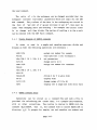
SECTION 3 - DETAILS OF HOW TO RUN THE PROCEDURES
ISIS computing system
Data files and Batch system
Instrument information
Overview of GENIE
Overview of procedures
Program NORM
Transmission routines
Program CORAL
Routine VANSM
Routine ANALYSE
Routines PLATOM and INTERFERE
Routine MERGE
Routines STOG and GTOS
APPENDICES
A
B
C
D
E
Resolution of a time-of-flight diffractometer
How to estimate the count rate of a diffractometer
Maximum entropy methods in neutron scattering:
application to the structure factor problem
Glossary of file extension names
Neutron absorption resonances
REFERENCES
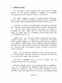
INTRODUCTION
The purpose of this manual is to describe a package of data
analysis routines which have been developed at the Rutherford Appleton
Laboratory for the analysis of time-of-flight diffraction data from
liquids, gases, and amorphous materials. It seemed to us that a
majority of users were put off analysing their data properly because of
the apparent complexity of TOF data, although in actual fact the basic
steps are the same as in a reactor experiment. Furthermore our
experience to date has shown that there really is no fundamental
barrier to diffraction data being accurately analysed to structure
factor or even pair correlation function within a very short time of
the completion of the experiment (always assuming the computer is "up"
of course!).
What has prevented this in the past has been a lack of
understanding of what to do with the data and how to do it. For our
part the relevant routines have been spread around different
directories with different modes of input and operation, which has led
to great inefficiencies for all concerned.
Therefore the package has now been set up with all the relevant
routines in a single area of the computer in such a way that it
requires a minimum of understanding of computing aspects on the part of
the users, at the same time as allowing them to check that each stage
of the analysis has been completed satisfactorily, and also enabling
them to re-sequence the steps or add additional ones according to their
own requirements. For example application of inelasticity corrections
and calculation of the pair correlation function tend to be
controversial stages with each user having his or her own preferences
for how they should be achieved. While the package supplies suitable
routines, the users can readily incorporate their own preferred
routines as necessary. At several points the package requires an
intelligent interaction with the user which means he or she is not
entirely free from responsibilities. Hopefully after studying this
manual he or she will be able to respond to the requests made of him
confidently!
The other guiding principle we have adopted is that the users will
not be willing to ship the very large raw data files generated in these
experiments, but on the other hand will be willing to remain a short
while at RAL after their experiments in order to complete the routine
analysis. In this way they can return home with the much smaller files
containing the structural information they are seeking for more
detailed manipulations at their home institutions. This makes sense
because most university users are not equipped to handle the size of
typical ISIS data files, nor provide the necessary archive which is
done at ISIS immediately after each run is completed. Having said that
however we also request that users do NOT use the ISIS HUB computer for
these subsequent manipulations because by doing so they simply slow
down the HUB for other users, who also can only afford to spend a
limited time at RAL analysing their data. Of course there are no
restrictions on those users ambitious enough to take the raw data home
and analyse it from scratch themselves: we will be happy to let such
people have copies of any of our routines that they might need.
The package has been developed primarily for analysis of ISIS data,
but is not limited to a specific instrument: the procedures will work
equally well on any ISIS diffractometer, although LAD is used as the
example throughout this manual. Because of its great versatility the
GENIE command language, invented by Bill David, or variants of it, is
used for the main stages. However the only stage which is strictly ISIS
specific is the very first in which the raw data in ISIS format are
converted into GENIE format. Therefore the package could in principle
be used at other institutions which have the GENIE language, the only
modification required being to the initial input of the raw TOF data.
Obviously while every effort has been made to ensure that the
routines do what we say they do, we can accept no responsibility for
errors which may occur: careful checking at each stage normally should
show up any errors. We would welcome suggestions for ways in which the
procedures can be corrected and improved.
This manual is in no way comprehensive. Further details are
contained in the papers referred to. In particular the reader is
encouraged t o read Colin Windsorts book, "Pulsed Neutron ScatteringN
[ll
SECTION 1
TINE-OF-FLIGHT DIFF'RACTION
page 1-1
1.1
THE TIME-OF-FLIGHT NEUTRON DIFFRACTION EXPERIMENT
There are seven principal components to a time-of-flight
diffraction experiment: (1) production of neutrons in a target, (2)
slowing down and thermalization in a moderator, (3) collimation of the
neutrons into a beam, (4) a sample to scatter the neutrons, (5) a
detector to analyse the tldiffractionw pattern of the scattered
neutrons, (6) a set of data acquisition electronics (DAE) with which
the data are stored, initially in fast memory and eventually on
computer memory, and finally (7) a data analysis package. Normally the
user is involved in providing the sample and performing the data
analysis, the rest being provided as part of the neutron facility.
Production of neutrons at a spallation neutron source is achieved
by accelerating bunches of protons to sufficiently high energies
(typically 500 - 800 MeV) that when they collide with a TARGET nucleus
they produce highly excited nuclear states which decay either
immediately or after a delay by throwing off nuclear particles such as
neutrons, y particles, neutrinos, etc. The maximum energy of neutrons
produced in this way corresponds to the energy of the impinging proton
beam, and if the target is uranium up to 30 neutrons per proton can be
produced. Other, non-fissioning targets such as tantalum or tungsten
produce about half this number of neutrons. The so-called "prompt"
neutrons are the ones used for time-of-flight analysis while the
"delayed" neutrons form a low level background in the diffractometer
which is independent of time, but must in general be corrected for as
it can be sample dependent. Normally the delayed fraction is on the
order of a few tenths of 1 percent of the prompt neutrons, but in cases
where an enriched booster target is installed, such as at the Argonne
National Laboratory in the U.S., this fraction can be higher.
The proton beam is pulsed so that a pulse of neutrons less that lps
wide is produced in the target. These neutrons are not useful however
page 1-2
because they typically have energies lo9 times too high for diffraction
effects to be seen. Therefore they are slowed down in a MODERATOR,
which scatters the neutrons many times before they escape. Light atoms
such as are in hydrogen-containing materials are used for the moderator
since the energy transferred ina collision is greatest when the two
particles have the same mass. Up to a point the thicker the moderator
the slower the neutrons become, but the process is self limiting,
because as well as slowing the neutrons down the moderator has the
effect of broadening the initial very narrow pulse significantly.
Therefore the moderator is designed to compromise between the
production of slow neutons and the requirements for reasonably narrow
neutron pulses: compared to a nuclear reactor the spallation target
would be regarded as under-moderated. The target-moderator assembly is
surrounded by neutron reflecting material, usually beryllium, to
enhance the neutron production and pulse shape.
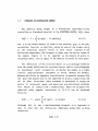
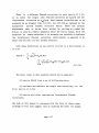
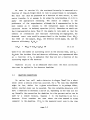
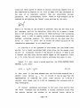
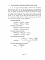
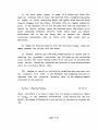
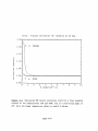
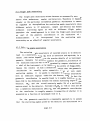
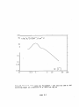
Figures 1.1 and 1.2 show a typical neutron spectrum from the
methane moderator at ISIS, plotted as a function of energy and
time-of-flight respectively. Two regions in the spectrum can be
identified, the epithermal region where the intensity varies as 1/E or
l/t, respectively, and a Maxwellian "humpll which occurs when the
neutrons in the moderator reach a temperature close to that of the
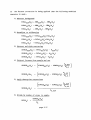
moderator. The neutron spectrum is therefore described by two functions
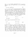
which are added together using a joining function [2]. The Maxwellian
region is described by the function
f a x(E)
=
J - exp{-E/T}
T~
while the slowing down epithermal region is represented by
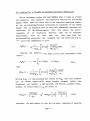
These two functions are combined by means of an empirical switch
function, A(E) :
page 1-3
where
In these equations J is the integrated Maxwellian intensity, T is the
effective temperature of the Maxwellian in enegy units, Qo is the
differential flux at 1 eV, A is a leakage parameter, and W1, W2 are two
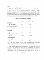
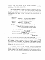
parameters which define the switch function. Table 1.1 lists the values
of these constants for the methane and ambient moderators at ISIS.
TABLE 1.1 ISIS moderator constants
*
Epithermal
Qo (at 750MeV)
CH4
Ambient H20
2.7
[1010n(e~sr100cm2~~s)~1]
A
0.92
Maxwellian
Joining function
1.7
4.0
7.0
10.6
W2
*N.B. The above numbers for Q0 refer to 750MeV proton energy. The
100cm2 refers to the area of the moderator normally viewed.
The neutrons emerge from the moderator in all directions and so to
be useful for diffraction they must be COLLIMATED. An essential
difference between TOF and reactor diffraction is that there is no
monochromator for the TOF experiment which means the full spectrum of
page 1-4
neutron energies, from 800 MeV downwards, is incident on the sample.
Therefore materials like cadmium and gadolinium which might be used in
a reactor situation are useless in the TOF case, and may even be
detrimental because of the high energy y's produced by neutron capture
in those materials. Instead boron, which has a l/v capture cross
section over a wide energy range, is the primary component, with large
amounts of iron and hydrogen (the latter usually in the form of wax or
resin) to provide the basic scattering cross section. Because the final
scattered intensities are small compared to the incident beam
intensity, and because it is essential to provide a radiation free
environment for people working near the diffractometer the TOF
collimator is a massive construction: at ISIS the collimator plus
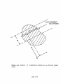
shielding measures typically -1.5m square. Figure 1.3 shows a diagram
of the prototype SANDALS collimator. This collimator is surrounded on
all four sides by about 0.4m of iron, and a further 0.3m borated wax
outside the iron.
The collimator defines a NEUTRON BEAM at the sample position. This
must be sufficiently well collimated to give adequate angular
resolution for the type of experiment being undertaken, but large
enough to give an acceptable count rate. Crystalline powder experiments
generally need high resolution in order to discriminate effectively
between adjacent Bragg reflections and also to determine the sample
constribution to the shape of individual reflections. However because
Bragg reflections are so sharp the count rate is rarely a severe
constraint, unless special effects are being determined, such as the
change in structure as a function of time. For liquids and amorphous
materials however the structure factor consists of a few broad peaks
which merge together, continuously. Detailed analysis of these requires
absolute measurements which can only be achieved through careful and
accurate measurements. In many examples, particularly those which
involve measuring changes in structure as a function of pressure,
temperature or isotope, count rate can be of paramount importance
because of the intrinsic weakness of the signal. Increases in
resolution can only be used if a count rate appropriate to the
resolution is available.
page 1-5
The SAMPLE is normally held in a CONTAINER: in addition if the
temperature is to be different from ambient then a FURNACE is required
to go above room temperature, and a CCR (CLOSED CYCLE REFRIGERATOR),
for temperatures down to -20K, or HELIUM CRYOSTAT, for temperatures
down to 4.2K, is required. Somewhat lower temperatures can be achieved
by pumping on the helium in the crystat.
For accurate structure factor measurements the mounting and
containment of the sample can be crucial since the diffractometer is
sensitive to small positioning offsets on the order of lmm. This
sensitivity arises from the small variations in final flight path and
scattering angle which can occur from one sample to another if each
sample is not placed in exactly the same position as its predecessor.
One solution to this difficulty which is applicable if the sample will
not be under pressure is to use a flat plate sample can with an area
larger than the beam area. This largely avoids the positioning
problems. In general however cylindrical cans must be used for pressure
or furnace experiments and so it is essential to ensure that if
cylindrical cans are used the sample positioning is accurate to O.lmm.
Ideally the container should be made of a purely incoherent
scattering material (vanadium or zirconium-titanium are the closest to
this ideal), otherwise the Bragg reflections from the container can be
hard to subtract completely: the problem arises because the front and
back of
the sample container correspond to slightly different
scattering angles at the detector so that Bragg peaks from front and
back arrive at slightly different times-of-flight. Thus when the
container is measured empty and then filled with sample the neutron
attenuation by the sample causes the Bragg peaks from the front of the
container to be attenuated preferentially compared to those from the
rear, causing an apparent shift in the position of the peaks in time.
Once again the ideal of an incoherent container may be hard to meet if
a particularly corrosive sample requires a special material for
containment. Fortunately zirconium-titanium alloy is suitable for many
pressure vessels.
page 1-6
The next diffractometer component, the DETECTOR, adopts one of two
3
forms. It is usually a gas proportional counter, with He gas the
primary neutron absorber, but at ISIS there has been considerable
development work on neutron scintillator detectors. If all goes well
the user should not have to be particularly concerned about which kind
of detector he is using, although he should be aware of its efficiency
and deadtime. The reasons for choosing scintillator detectors for
liquids and amorphous materials centre on their much lower cost,
compared to He tubes, and on the fact that they can be made at least
twice as efficient as the He tube. In this way the epithermal part of
the neutron spectrum can be used more effectively.
The primary object of the DATA ACQUISITION ELECTRONICS, DAE, is to
record each neutron event and give it a label corresponding to the
number of the detector in which it occurred and to the time of arrival
at the detector. The clock which measures this time of arrival is
started by an electronic pulse which is generated when a burst of
protons hits the target. At ISIS this occurs 50 times a second. Once
the label is generated, a word of memory corresponding to the label is
incremented. In this way a histogram of events is built up. The
experiment is controlled by a FRONT END MINIcomputer (FEM) which is a
computer to store, manipulate and display the data.
After transmission through the sample the neutrons and other
particles are absorbed in a BEAM STOP, which again at ISIS is of a
massive construction, as it must absorb all potentially dangerous
particles which come down the beam line. In fact different pulsed
neutron sources have adopted different modes of operation: at the
HARWELL linac and at the LANSCE facility at Los Alamos, parts of the
facility are inaccessible while the beam is on, in order to protect
experimenters from radiation exposure. At ISIS on the other hand the
shielding is sufficiently comprehensive that even when running at full
power the background radiation levels are certainly low enough for
people to remain near the diffractometers for extended periods.
page 1-7
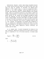
The time of arrival, to, of a neutron at the detector is given by
its "TIME-OF-FLIGHT", TOF, which is the time (in us) taken by the
neutron to travel lm, multiplied by the total total flight path in m.
Several useful relationships can be written down between the neutron's
time of flight TOF (dm), velocity v (in m/s), wavelength X (in A),
wavevector (in
X
(A)
=
A-l)
and energy E (in meV). Thus
0.0039562TOF
=
0.0039562tO(vs)/L(m)
Using these relationships we can write down the incident flux
distribution as a function of wave vector or wavelength in terms of the
energy distribution:
((k)
=
;(
4 )
=
24(E)
kj,
etc.
Note that since in the epithermal region 4(E) = %/E,
@(A)
=
2aO/X, P(k)
=
then
2eO/k, etc.
An important characteristic of any diffractometer is its resolving
power: it is the Q-RESOLUTION which makes the primary distinction
between a powder diffractometer, where there are many sharp peaks close
together and so requires high resolution, and the liquids and amorphous
diffractometer where
the peaks are broader, merge together
continuously, and hence requires relatively low resolution. For liquids
and amorphous materials diffraction, irrespective of whether it is
constant wavelength or time-of-flight diffraction, the scattered
intensity, which is proportional to the structure factor S(Q) (see
section 1.2, is measured versus the momentum transfer, RQ, where for
elastic scattering
page 1-8
Q
=
4rt sin 8 /
X
(1.1.7)
28 is the scattering angle and X the neutron wavelength. In the case of
TOF, X is measured by time-of-flight with 8 held constant. In that case
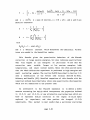
we see that the resolution, AQ, has two components:
The wavelength uncertainty, A M X , arises from the intrinsic pulse width
of the incident neutron beam and from the flight path uncertainty to
the detector, &/L, where L is the total flight path from moderator to
detector. A more detailed account of contributions to the resolution
function is given in Appendix A. We note that for a given TOF channel
the width of the pulse, Av, as a function of neutron velocity, v, is
proportional to v, i.e. Av/v = A M X = constant. Similarly since for a
given time channel
it will be seen that the flight path uncertainty also gives rise to a
wavelength uncertainty such that A M X = &/L = constant as a function
to. Hence we see from (1.1.3) that the resolution nQ/Q is roughly a
constant as a function of TOF for a given scattering angle.
Further details about the effects of resolution are given in Appendix
A. The count rate on a diffractometer is denoted by its "count rate
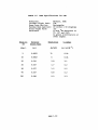
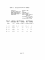
number" or "C-number" (see Appendix B for details). Table 1.2 lists the
resolutions and C-numbers for LAD and Table 1.3 lists the projected
numbers for SANDALS.
page 1-9
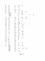
TABLe 1.2
Some Specifications for LAD
Moderator:
Methane, 100K
Incident Flight Path:
10m
Beam Cross Section:
Rectangular
Maximum Beam Aperture: 20 (wide) x 50 (high)mrn
Final Flight Path:
-1m
Detectors:
10 atm He detectors at
5O, lo0 and 150°,
Li-glass scintillators at
other angles.
Range In
28
Detector
Solid Angle
Resolution
page 1-10
C-number
TABLE 1.3
Some Specifications for SANDALS
Moderator:
Incident Flight Path:
Beam Cross Section:
Maximum Beam Aperture:
Final Flight Path:
Detectors:
Methane, 100K
llm
Circular
32mm (diameter)
0.75111- 4.0m
Zinc sulphide sandwich
detectors
200 (high) x 10 (wide)
x 20 (deep) mm
30% efficient at lOeV
Range In
Detector High Resolution
20
Solid Angle Res.
C-number
page 1-11
Low,Resolution
Res.
C-number
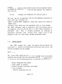
1.2
OVERVIEW OF DIFFRACTION THEORY
The quantity being sought in a diffraction experiment on any
crystalline or disordered material is the STRUCTURE FACTOR, S(Q), where
S(Q)
=
I
1 + p dy (g(5)
-
1) exp(iQ.r)
--
(1.2.1)
and p is the number density of atoms in the material, g(r) is the pair
correlation function at position r given an atom at the origin, and Q
is the reciprocal lattice vector or wave vector transfer in the
diffraction experiment. The integral is taken over the entire volume of
is to be regarded as the density of points in
the sample. S(Q)/p
) is the density of points in real space.
reciprocal space, just as pg(rThe definition of the structure factor (1.2.1) although different
from the normal definition for structure factor used in crystallography
is nonetheless valid irrespective of whether the sample is a single
crystal, polycrystalline, amorphous or fluid. However for powders,
)
glasses and fluids an immediate simplification is possible because S(Qand g(r) then depend only on the magnitude of Q and r respectively and
not on their directions. (This statement is equivalent to saying the
points in reciprocal space and space real are distributed uniformly
into shells of radius Q and r respectively). Hence the integral over
spherical polar angular coordinates in (12.1) can be performed
directly:
s(Q)
=
1 + 4np/Q
rdr (g(r) - 1) sin(Qr)
(1.2.2)
Although this is now a one-dimensional integral, it is important to
bear in mind that the diffraction experiment probes S(Q) in three
dimensions.
page 1-12
For a multicomponent system there is a term like (1.2.1) or (1.2.2)
for each distinct pair of atomic types, a,B; all the partial structure
factors, S (Q), are summed together in the TOTAL STRUCTURE FACTOR with
aB
weights proportional to the product of the scattering lengths for each
atomic type:
where ca is the atomic fraction, ba is the scattering length, of
element a, and the bars indicate averages over the spin and isotope
states of each element, assuming of course these are not correlated
with position. The first term in (1.2.3) is called the "SELFu or
"SINGLE ATOM" scattering, while the second is called the "INTERFERENCE"
or "DISTINCT" scattering, because it contains the basic structural
information on atomic positions.
The quantity measured in a neutron diffraction experiment is
strictly NOT the structure factor, but the DIFFERENTIAL CROSS-SECTION,
which is defined as
do
,-ii(X,28)
I
umber of neutrons scattered per unit time
the small solid angle dP at angle 28
=
N @(A) dP
(1.2.4)
where N is the number of atoms (or scattering units if such a
definition is more convenient) in the sample, and @(A) is the incident
neutron flux at wavelength A. As for the structure factor the
differential cross-section can be split into "self" and "distinctn
terms:
In the absence of any corrections for attenuation, multiple scattering
page 1-13
and inelasticity effects the differential cross section is equal to the
total structure factor, F(Q). This known as the STATIC APPROXIMATION.
In particular the self and distinct parts are defined as
and
In neutron scattering the nucleus recoils under neutron impact and
so the neutron can exchange energy with the scattering system (an
IfINELASTIC" collision. Hence even with diffraction experiments dynamic
effects almost invariably have to be considered. These are described by
the van Hove dynamic structure factor, S(Q,o), [ 3 ] , with separate terms
for self and interference scattering as before. The single atom term
for atom a will be represented here by Sa(Q,w), and the interference
term between a and B by S (Q,o). In terms of these quantities the
aB
so-called "STATIC STRUCTURE FACTORS" are defined by
sa(Q)
=
sap-1
=
j sa(O,m)
dw
const Q
.
=
1.
SaB("m)
d~
-m const Q
where the integrals are taken along a path of constant Q. It will be
readily apparent that the diffraction experiment ideally should
integrate S(Q,w) over all energy transfers and so obtain an ensemble
averaged "snap shottfview (t=O) of the material. It is quite different
from the ELASTIC diffraction experiment which probes only S(Q,O) and so
determines the residual structure after waiting a long time (t=m).
.
page 1-14
In terms of these partial dynamic structure factors the total
dynamic structure factor for a material is defined in the same way as
(1.2.3):
The inelasticity associated with the scattering causes a particular
effect in that neutrons can arrive either earlier or later than they
would have done if the scattering were elastic (no exchange of energy).
If k and k t are the neutron wavevectors before and after the scattering
then the TIME-OF-FLIGHT EQUATION states that
where L is the incident flight path, moderator to sample, L' is the
flight path sample to detector, and ke is the elastic wavevector for a
particular time channel. The TOF equation combines with the usual
kinematic equations for the neutron:
and
to define the path through (Q,o) space over which F(Q,o) is integrated.
Hence instead of measuring (1.2.3) for the sample directly, as we would
ideally like to do, the TIME-OF-FLIGHT DIFFERENTIAL CROSS SECTION,
TDCS, is obtained in practice:
c(Qe,e)
do
=
(1.2.12)
where @(k) is the incident spectrum expressed as a function of k, as
described in section 1.1, E(kt) is the detector efficiency at the final
page 1-15
final wave vector, ke is the wavevector for elastic scattering, and Qe
= 2k sine. The dependence of C on 8 as well as Q is shown to emphasize
e
that for a given Q value the TDCS is still a function of scattering
angle. The partial derivative can be evaluated using 1.2.11 in 1.2.9:
where R = Lf/L. Egelstaff [4] calls this a "sampling factor" because it
controls the way F(Q,o) is sampled.
Note that the TDCS is to be distinguished from the differential
cross section (1.2.4) by virtue of the finite final flight path: if R
were to go to zero then the TDCS is identical to the differential cross
sention. The denominators in equation (1.2.12) imply that the measured
data have been normalized to the incident beam and detector
efficiencies at the elastic energy. This is achieved in practice by
dividing the TOF data by the scattering from a standard sample, usually
vanadium, which scatters almost entirely incoherently. Even so some
spectrum dependence is found in the TDCS because of the inelastic
scattering of some detected neutrons.
Strictly speaking the integral in (1.2.12) implies we cannot do the
experiment because we don't know F(Q,o), and even if we measured it we
could never obtain it over wide enough w range to perform the integrals
in (1.2.4) accurately. However, as has been shown by Placzek [5] and
many others since then [e.g.4,6-131, the difference between F(Q) and
Z(Q,e) is small enough in many cases that we can estimate the
difference
by using an approximate model for F(Q,u). For example such a model
might satisfy the first two moments of the true F(Q,w), which are often
known. P(Q,8) is called the PLACZEK or INELASTICITY CORRECTION, and
note that it too is a function of both Q and 8.
page 1-16
There is a different Placzek correction for each term in (1.2.3),
so we label the single atom Placzek correction as Pa(Q,O) and the
interference correction as P (Q,O). Each Placzek correction has to be
a6
evaluated by an integral like (1.2.12), but with F(Q,o) replaced by the
appropriate partial dynamic structure factor. There are several
approximate ways of doing this, either by putting in a model for
S(Q,w), or else by a Taylor expansion about the static values. With the
exception of simple molecules it is normally not possible to evaluate
the interference Placzek correction, which however is expected to be
small (see section 2.10 for further details).
With these definitions we can rewrite (1.2.12) in a form similar to
(1.2.3):
The basic steps in data analysis should now be apparent:
(1) derive C(Q,O)
from a set of diffraction data;
(2) estimate and subtract the single atom scattering, i.e. the
first term in (1.2.15);
(3) derive g(r) after removing any interference Placzek
corrections.
The bulk of this manual is concerned with the first of these steps,
although we will also suggest ways of tackling the other two stages.
page 1-17
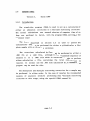
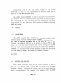
T I T L E : Neutron spectrum v .
energy
Figure 1.1 Time-of-Flight neutron spectrum as a function of energy.
Note the log scales used in the graph
page 1-18
Figure 1.3 Diagram of the prototype SANDALS collimator illustrating the
bulkiness of neutron shielding at ISIS.
page 1-20
SECTION 2
STEPS IN DATA ANALYSIS OF TOF DIFFRACTION DATA
page 2-1
2.1
INTRODUCTION
The initial goal of the experimenter is to obtain the TDCS of his
or her sample. The success of subsequent analysis to g(r) or partial
structure factors depends critically on obtaining the TDCS accurately.
A number of corrections are required to the measured data: these are
straightforward to apply but nonetheless easy to get wrong. Four main
sources of error can be identified:
(i
the experimenter doesn't have complete
information about his or her sample, e.g.
dimensions, densities, cross sections, etc.;
(ii)
incorrect data analysis procedures are used;
(iii)
the detectors are not sufficiently stable;
(iv)
sample environment equipment introduces
unexpected backgrounds and sample positioning
errors.
The last two causes require action by the instrument scientists, but
there is little or nothing that can correct for poorly characterised
samples or incorrect data analysis procedures.
Occasionally on LAD we have achieved absolute accuracies of 1%,
accuracy being measured by the difference between the measured high Q
limit of the TDCS and the expected high Q limit. With care this
accuracy could be achieved routinely. However at present we typically
obtain accuracies on the order of 5%, and in the majority of cases the
reason for this is either because the sample is poorly characterised or
because the data analysis is inadequate.
With the exceptions of sections 2.9 and 2.11, which concern the
estimation of inelasticity corrections and transforming the final
result to g(r), we believe the methods of analysis of diffraction data
from liquids and amorphous samples are well understood and routine. In
the sections which follow we have attempted to describe the correct
sequence of steps.
page 2-2
As seen in section 1.1, the scattered intensity is measured as a
function of time-of-flight which in turn is proportional to wavelength.
The data can also be presented as a function of wave vector, k, wave
vector transfer, Q, or energy, E, by using the relationships (1.1.5) to
apply the appropriate rescaling. The choice is subject to the
preference of the experimenter, although the Q representation is the
most common as it relates to the reciprocal space in which the
structure factor is defined, equation (1.2.1). Therefore we shall use
the Q representation here. Thus if the sample is very small so that the
effects of attenuation and multiple scattering are negligible, the
detected count rate would be proportional to the incident flux, @(ke)
the TDCS of the sample, C(Qe), the detector solid angle, AR, and the
detector efficiency, Ed(ke):
where N is the number of scattering units in the neutron beam, and Qe =
2kesin0. The incident flux and detector efficiency are represented here
as a function of ke to emphasize that they are not a function of the
scattering angle of the detector.
Equation (21.1) is an idealized count rate: the first correction
that must be applied is for detector deadtime.
2.2
DEADTIME CORRECTIONS
No matter how well made a detector is always "dead" for a short
while after a neutron event has occurred. For a 3He tube this DEADTIME
might be 3us, whilst for a glass scintillator it is perhaps 250ns,
before another event can be recorded. The zinc sulphide detectors will
have a deadtime of betweeen 2 and 10 us, depending on how they are set
up. Normally the correction for deadtime is a few percent and so can be
made by a simple formula. Suppose T is the deadtime in us for a
detector. First consider the case where the time channel is broad
compared to the deadtime. If Rm is the measured count rate in the time
page 2-3
channel (in cts/vS), then the detector is dead for a time
where A is the width of the time channel in US. Hence the count rate,
R, which would have been measured if the detector had zero deadtime, is
greater than Rm in proportion to the time that the detector is dead:
At the other extreme if the time channels are narrower than the
deadtime, then some of the previous time channels may contribute to the
deadtime in a particular channel. For example if channels n to m
contribute to the deadtime in channel m, then the length of time
channel m is dead is given by
where A and R are the channel width and count rate in channel j
j
j
respectively. The limits of j are determined by inspection. This
correction is used in the same way as before, with Dm in place of D in
(2.2.2).
A subtlety occurs in practice that renders,the correction more
complicated. When many detectors exist it is not practical to have a
separate input for each detector into the DAE. Instead an ENCODER is
used to create a binary address which describes which detector fired.
If the deadtime of the encoder is longer than that of the detector,
then it is the encoder's deadtime which determines the detector
deadtime. Moreover since the encoder can process only one event at a
time, all the detectors that feed into that encoder are effectively
dead when any one detector fires. Therefore in this situation the sum
in (2.2.3) should include a sum over all channels which feed into a
decoder. In that case if R
is the count rate in time channel j and
j ,k
encoder channel k, then the detector deadtime is given by
page 2-4
and the sum over k is over all detector channels that feed into the
encoder. In the situation when (2.2.4) applies A. is the encoder's
J
deadtime, NOT the detector's. Hence even though the deadtime for an
individual detector may be small, the grouping of say 50 detectors into
an encoder results in a 50-fold enhancement in the count rate as far as
deadtime is concerned. So the deadtime correction could be much larger
than might be apparent from the count rate in an individual detector.
2.3
NORMALIZING TO THE INCIDENT BEAM MONITOR
Having corrected I(Qe) for deadtime, the next stage is to divide
out the incident spectrum, which is measured by means of a MONITOR
detector placed in the incident beam before the sample. The spectrum is
divided out at this stage because small variations in moderator
temperature and proton beam steering can modify the energy dependence
of the spectrum from time to time at the 1-2% level. Since the
calibration run must be performed before or after the sample run, it
will only give a reliable result if the dependence on the incident
spectrum is removed at the end of each run. The count rate in the
monitor detector, which of course must also be corrected for deadtime,
is proportional only to the incident spectrum and the monitor
efficiency:
Thus when used to normalize the scattered neutron count rate, a
NORMALIZED count rate is obtained:
page 2-5
A second measurement which is made at the same time as the
scattered count rate from the sample is the fraction of neutrons
transmitted by the sample. This number is monitored by a TRANSMISSION
MONITOR, with efficiency Et(ke), placed after the sample. Again this
fraction cannot be measured directly, but must be determined by
ratioing different runs, e.g. with and without sample. If It(ke) is the
count rate in the transmission monitor, then this count rate is
proportional to the incident flux, the transmission monitor efficiency
and the TRANSMISSION of the sample, T(ke), which will be defined in the
next section and is dependent on the total neutron cross section of the
sample. Hence when normalized to the incident monitor, the transmitted
intensity is given by
The transmission monitor is used to provide information on the neutron
cross section and density of the sample: it can often confirm that the
sample is what it is supposed to be.
There will then be a set of NRM files for every detector or
detector group, and a MON file, for every run, whether it be sample,
container, vanadium (calibration) or background. The stages covered by
sections 2.2 and 2.3 are obtained by running the NORM program of
section 3.6
2.4
MEASURING THE NEUTRON CROSS SECTION
a) The Total Neutron Cross Section
Neutron cross sections arise from two primary processes: scattering
and capture. Provided there are no nuclear resonances in the energy
region of interest, the probability for capture is inversely
proportional
to neutron velocity, i.e. proportional to neutron
wavelength, and the constant of proportionality, usually defined for
2200m/s neutrons ( A
=
1.8A), is called the CAPTURE CROSS SECTION, ua.
page 2-6
There is a value of ua for every nucleus, although in many cases it is
quite small or zero.
The SCATTERING CROSS SECTION, %(A),
on the other hand has no such
simple dependence on energy or wavelength, because it represents the
integral of the DIFFERENTIAL SCATTERING CROSS SECTION, du/dQ at a
particular wavelength over all scattering angles:
us(X)
=
I
-J$X) dQ
=
4n
sin 28 dB
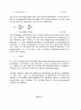
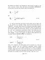
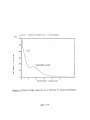
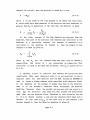
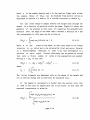
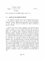
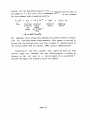
As an example of the application of this result we will assume the
static approximation applies and that the liquid under inverstigation
is a hard sphere fluid of reduced density pu3 = 0.5, where u, the hard
core diameter, is 3.142A. In that case S(Q) is known exactly in the
Percus-Yevick approximation, and so (2.4.1) can be integrated
numerically for all wavelengths, using
where b is the bound scattering length of the fictitious nucleus. The
result is shown in figure 2.1: it will be seen that the scattering
cross section for a material with structure will certainly deviate from
the bound value. In particular the scattering cross section will
display a similar structure to that seen in the differential scattering
cross section.
For light atoms such as hydrogen and deuterium the consequences are
quite drastic: the differential cross section falls dramatically with
scattering angle at all but the longest neutron wavelengths, and the
shape of the fall, which depends on the details of S(Q,u), also varies
with energy. Thus at low energies the neutron can excite only
diffusional type motions, while at high energies the neutron can excite
all possible modes, including dissociation of molecules if present.
Thus the scattering cross section must vary between its so-called
"BOUND" and "FREE" values as we go from low energy to high. The llboundw
page 2-7
values are those quoted in tables of neutron scattering lengths such as
the compilation by Koester et. al. [14] or Sears 1151 and correspond to
the case of an immovable nucleus: they are essentially nuclear
parameters. The corresponding l1freel1 values at high energies can be
computed by multiplying the llboundllcross sections by the ratio
where A is the mass of the nucleus in question. This has the value 0.25
for hydrogen and 0.44 for deuterium, which tells us to expect a large
fall in the scattering cross section of these materials with increasing
energy. Such a fall is readily visible in the transmission data from
hydrogen containing samples. For heavy atoms on the other hand this
factor is close to unity and so within the likely accuracy of the
transmission measurement is not significant.
In practice it is not possible to ever obtain the true bound cross
section for a liquid containing light atoms since the low energy cross
section is intimately related to the details of S(Q,w) at small Q and
o. However the free cross section should appear as the asymptotic limit
as X * 0, since then all neutron capture processes have gone to zero.
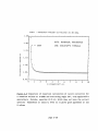
Figure 2.1 also shows a second quantity, the TOTAL NEUTRON CROSS
SECTION, at(A), where
In this case it has been assumed that the fictitious material has a
capture cross section ua = 0.4 at ~=i.8A. It can be seen that the
approximation of treating the total cross section as a sum of a
constant plus linear term in X will be inadequate for accurate work at
long wavelengths.
If nuclear resonances are present in the total cross section then
the above treatment must be modified. A nuclear resonance occurs when
the neutron excites the nucleus to an excited state, and so is
page 2-8
(slightly) analogous to an absorption edge in X-ray scattering. However
the possible nuclear states are quite complicated in general and can
be accompanied by several processes, including the emission of a y
photon. Usually both scattering and capture are not simple at a
resonance, and full treatment of the effects of this on the data
analysis are beyond the present purpose, and certainly are not included
in any of the correction routines. At present the only recourse is to
ignore the energy regions where resonances occur and hope that there is
sufficient angular coverage that all Q values can be obtained away from
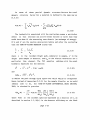
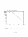
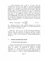
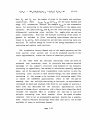
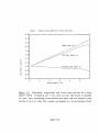
a resonance. Figure 2.2 shows the measured total cross section for a
solution of 148~m-perchlorate in D 2 0 Note the strong resonance at X =
lA, corresponding to a nuclear resonance in a 14'sm
impurity. This
resonance was so broad that analysis of these data to TDCS was
impossible. Appendix E lists the more commonly occurring resonances.
b) Measuring the Neutron Cross Section
We have seen above that the total cross section depends on the
STRUCTURE and DYNAMICS of the sample, which in turn relates to the
thermodynamic state of the sample. Therefore it strictly has to be
measured for each and every sample, and this is why a transmission
monitor is placed after the sample. In practice it is difficult to
measure the total cross section on an ABSOLUTE scale with the necessary
precision, so the transmission monitor is used to obtain the ENERGY
DEPENDENCE of the total cross section, with absolute values obtained by
reference to the known free and bound values at short and long
wavelengths. Note
that using a separate experiment to measure
transmissions is very time consuming and not necessarily useful since
it is not always possible to reproduce the exact conditions of the
experiment at a later time.
If the sample is a flat plate which uniformly covers the beam then
the TRANSMISSION of the sample is given simply by
page 2-9
where p is the number density and L is the neutron flight path within
the sample. Hence if T(ke) can be obtained from monitor ratios as
described in section 2.3 then it is a trivial inversion to obtain ut.
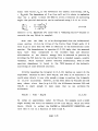
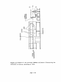
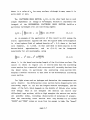
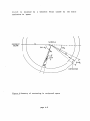
For any other shape of sample however the flight path through the
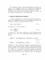
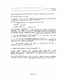
sample is a function of position within the beam. Figure 2.3 shows the
geometry of the problem in this case.. If x measures the perpendicular
distance from one edge of the beam then L becomes a function of x and
the transmission in this case can be written as
where W is the
width of the beam. In this case there is no simple
inversion to ut, which has to be obtained by trial and error. However
if a Newton-Raphson technique is used to do this convergence to a
solution is quite rapid. Further efficiency can be gained by noting
that only a finite number of terms in the exponential are needed.
Writing v = pu we see that
t'
where
/
w
The latter integrals are dependent only on the shape of the sample and
not on neutron energy and so need only be evaluated once.
If the sample is contained in a holder then the monitor ratio that
is used is the ratio of sample plus can to can alone. In that case the
measured transmission is given by
page 2-10
where the capital suffix S applies to the sample and C applies to the
container. Similar expansions of the top exponential term can be used
as before. However the values of pC must be supplied separately or
obtained in a separate transmission experiment on the container alone.
Finally note that if the beam profile is not uniform a simple
modification of the above formulae is needed: because the profile
function can be included in the moments (2.4.7) it does not lead to any
increase in computing time.
2.5
ATTENUATION AND MULTIPLE SCATTERING CORRECTIONS
Much of the underlying methodology for calculating ATTENUATION and
MULTIPLE SCATTERING corrections has been covered in numerous previous
publications and so will not be repeated here. Although there are a
number of approaches to the calculation, the formalism of Soper and
[16], which
uses numerical integrations to estimate
Egelstaff
corrections for the cylindrical geometry, is used here, because it is
written in a sufficiently general form to allow corrections for
furnaces and radiation shields if they are sufficiently absorbing or
scattering to require a separate correction. These latter corrections
will be the subject of the next section.
The most common case is that of a sample contained in a holder. In
that case two measurements are needed: one for the sample plus can,
ISC(ke),
and one for the can alone, IC(ke). These two quantities are
each affected by attenuation and multiple scattering so our simple
definition (2.1.1) has to be modified for the general case:
page 2-11
Here NS and NC are the number of atoms in the sample and container
AS,SC, AC,SC and A
are the usual Paalman and
respectively, while
C?C
Pings [17] attenuation factors. For example AS,SC is the attenuation
factor for scattering in the sample and attenuation in the sample plus
container. The quantities MSC and MC are the total multiple scattering
differential scattering cross sections for sample plus can and can
alone respectively. Note that the multiple scattering terms cannot in
general be included in first scattering terms because they are not
linear in NS and NC ' Both attenuation and multiple scattering terms are
functions of neutron energy by virtue of the energy dependence of the
scattering and capture cross sections.
The attenuation factors depend only on the sample geometry and the
total neutron cross section and so can be evaluated exactly in the
static approximation, within the limits of numerical precision.
On the other hand the multiple scattering terms can never be
evaluated very accurately since in principle they require detailed
knowledge of the sample's structure (and dynamics if the inelastic
scattering is significant). The method of calculation normally employed
makes use of the measured total transmission cross section to give the
scattering cross section at each neutron energy, but then assumes the
scattering at this energy to be isotropic with scattering angle. This
is called the ISOTROPIC approximation. (This is NOT the same as
assuming that the multiple scattering is isotropic, an approximation
introduced by Blech and Averbach 1181 which is not needed in practice.)
Sears [I91 has described how the isotropic approximation can be
improved although direct calculation with a Monte Carlo algorithm which
includes the measured TDCS is probably the best way to cope with
multiple scattering from thick samples. Given the speed of modern
computers this is not an unreasonable approach. Howells has a program,
ELMS, (Elastic Multiple Scattering) which does this and it can be made
available if there is sufficient demand.
page 2-12
There is a general consensus that the isotropic approximation is
expected to be acceptable if the sample scatters less than -20% of the
incident beam, although there has never been a quantitative study of
the size of sample at which this approximation starts to introduce a
serious systematic error in the measured structure factor. Clearly it
greatly assists the multiple scattering problem if the container can be
made
of
an
incoherent scatterer, such as vanadium or
zirconium-titanium, or of an amorphous material, such as silica, since
Bragg peaks introduce a severe difficulty to any quantitiative multiple
scattering calculation.
In summary, to be confident that multiple scattering will not
introduce too large a systematic error it is a useful rule of thumb to
ensure that the sample scatters between 10% and 20% of the incident
neutron beam.
2.6
FURNACE CORRECTIONS
If the sample and container are in a furnace and the furnace
element contributes significantly to the attenuation and scattering
processes then three measurements are needed: sample plus can plus
empty can plus furnace, ICFke), and furnace alone,
furnace, ISCF(ke),
IC(ke).
These three quantities are related to the corresponding
differential cross sections by:
page 2-13
The attenuation factors have the same definition as before, e.g.
As,SCF is the attenuation factor for scattering in the sample and
attenuation in the sample, can and furnace. Similarly the multiple
scattering cross sections have an equivalent definition as before. N~
is the number of furnace atoms in the incident beam.
2.7 VANADIUM OR STANDARD SAMPLE CALIBRATION
A unique characteristic of neutron scattering is the ability to
perform an independent estimate of the instrumental calibration. This
calibration consists of the unknown quantities, either
in sections 2.1, 2.5 and 2.6 above, or
Ed(ke)
F2(ke) =
ASZ
Em(ke)
in section 2.3. With
equations (2.5.1) and
monitor:
these definitions we can for example rewrite
(2.5.2) which become, after normalizing to the
Estimation of these calibration constants is usually achieved with a
standard vanadium sample because vanadium has a largely incoherent
cross section and so it is believed that the differential cross section
for vanadium can be estimated reasonably accurately, an assumption
which of course is difficult to check! As described in section 2.9 the
inelasticity correction has two principal terms, one relating to
page 2-14
scattering angle, the other proportional to temperature and inversely
proportional to neutron energy, and since energy is being varied in a
TOF experiment it is crucial to estimate this latter term correctly.
Figure 2.4 shows the estimated single atom differential cross section
scattering angle for a free vanadium nucleus at two
at 20°
temperatures. At the time of writing experiments are planned on LAD to
determine if the estimated temperature dependence is indeed observed.
The normalized spectrum from vanadium is defined by
brackets is the vanadium differential
The quantity in square ([...I)
cross section which is estimated using exactly the same methods as in
the previous section. This leads to a VANADIUM CALIBRATION, CALV(Qe),
where
In fact scattering from vanadium exhibits the usual statistical
noise plus weak Bragg reflections due to the small coherent scattering
amplitude. Since the data from the sample must be divided by CALV i t is
obviously undesirable to transfer either effect to the sample data, so
an expansion in terms of Chebyshev polynomials is fitted to NRMV with
zero weighting of points in the region of Bragg peaks. This has the
effect of smoothing out the Bragg peaks and noise without introducing
any appreciable artifacts. However it is clearly important to check
that this smoothing has in fact removed only the noise from NRMV and
none of the underlying structure. In any case whether to smooth or not
is an option which can be overridden if needed. The computer programs
associated with this section are described in section 3.9.
page 2-15
2.8
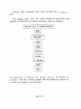
BASIC ALGORITHM TO DETERMINE DIFFERENTIAL CROSS SECTION
All of the main quantities needed to calculate the differential
cross section (DCS) from the TOF diffraction data of the sample have
now been described, and the algorithm ANALYSE (see section 3.10) is
used to perform this operation. The stages are described in sequence
for the case of a sample held in a can. Note that the arrow * is used
to indicate that the result of an operation on the left hand side is
placed in the quantity on the right. The symbol TOTAL applies to the
total scattering, SINGLE applies to single scattering, and the suffixes
S, C and B refer to sample, can and background.
1) Subtract background
TOTALSC(Qe)
=
mMSC(Qe) - mMB(Qe)
TOTALC(Qe)
=
mMC(Qe) - mMB(Qe)
2) Normalize to calibration
TOTALSC(Qe)
TOTALC(Qe)
* TOTALSC(Qe) /CALV(Qe)
* TOTALC(Qe)/CALV(Qe)
3) Subtract multiple scattering
SINGLESC(Qe)
=
TOTALSC(Qe) - MSC(ke)
SINGLEC(Qe)
=
TOTALC(Qe) - MC(ke)
4) Apply absorption corrections
5) Divide by number of atoms in sample
page 2-16
If the furnace correction is being applied then the following modified
sequence is used:1) Subtract background
TOTALSCF (Q,)
=
mMSCF ( Qe ) - m M B ( Qe )
TOTALCF(Qe)
=
mMCF(Qe)
TOTALF(Qe)
=
MMF(Qe) - NRMB(Qe)
- mMB(Qe)
2) Normalize to calibration
TOTALSCF ( Qe
TOTALCF(Qe)
TOTALF (Q,)
* TOTALSCF( Qe /CALV( Qe)
* TOTALCF(Qe)/CALV(Qe)
* TOTALF(Qe) /CALV(Q,)
3) Subtract multiple scattering
SINGLESCF(Qe)
=
TOTALSCFF(Qe) - MSCF(ke)
SINGLEcF(Q,)
=
TOTALCF( Qe) - MSC(ke)
SINGLEF(Qe)
=
TOTALF(Qe) - MF(ke)
4) Subtract furnace from sample and can
5) Apply absorption corrections
- SINGLEC(Qe)
S ,SCF
H
5) Divide by number of atoms in sample
page 2-17
SCF
A ~CF,
1
2.9
INELASTICITY (PLACZEK) CORRECTIONS
Equations 1.2.9, 1.2.11 and 1.2.12 serve to define the inelasticity
correction, P(Qe,6) in a TOF diffraction experiment: P(Qe,B) represents
the difference between the static approximation F(Q) and the TDCS,
C(Qe).
Strictly speaking to obtain P(Qe,B) one needs to know F(Q,m)
which preempts the need for a diffraction experiment since then the
static structure factors (1.3.4) would be obtainable by direct
integration of F(Q,o).
Obviously this is an impractical proposition,
mostly because of the time that would be required in measuring the
complete dynamic structure factor.
However in 1952 Placzek [5] showed that for nuclei much more
massive than the neutron the correction adopts a form which is
essentially independent of the detailed dynamics, and is related only
to the nuclear mass, the sample temperature, the incident neutron
energy, and the geometry and efficiency of the neutron detection
process. Moreover at neutron energies well above those of any bound
states that occur in the sample he showed that the correction to the
interference term S (Q) is zero to first order. These conclusions
aB
arose from the fact that the first two moments of S(Q,m) can be
estimated more or less exactly:
and
Here (2.9.1) and (2.9.3) are exact results, but (2.9.2) strictly only
applies to a classical fluid.
page 2-18
Unfortunately Placzekts results cannot always be applied directly
to thermal neutron diffraction because the conditions under which they
apply are often not obtained. In particular the sampling factor
(equation 1.2.10) rapidly drops to zero as k' becomes less than k.
Hence as in the fixed wavelength reactor experiment the scope for
exciting high vibrational levels in a molecule depends on the incident
energy. There is an extensive literature on the attempts to modify the
original Placzek approach to include the cases where the system is only
partly excited by the neutron. See for example the papers by Powles
[6-111 and Egelstaff [4,12,13] and references therein. All of these
involve lengthy algebra, and while there seems to be general agreement
in the case of the self scattering for an atomic fluid the correct form
of the terms for molecules, which involve a Q-depedent effective mass
is still disputed. The advantage of the Placzek type of expansion is
that in enables one to understand by inspection the effect of various
instrument parameters on the inelasticity correction, in particular the
flight path ratio, sample temperature, detector efficiency, and
incident spectrum shape,.
As an example below is quoted the Egelstaff [4] formula for the
self scattering inelasticity correction for an atomc fluid of nuclear
mass M at temperature T, for a 1/E incident spectrum, at incident enrgy
Eo :
where
page 2-19
and y = sin28, m
detector constants:
=
mass of neutron, a
=
1/R
=
L/Lt, and A and B are
with
Ed(ke)
=
1 - exp(-o/ke)
and E a detector constant which determines the efficiency. Further
terms are needed in the Maxwellian region.
This formula gives the quantitative behaviour of the Placzek
correction at large neutron energies, but also indicates qualitatively
what will happen at all energies. In particular we see that the
correction gets notably larger at low neutron energies, high
temperatures, and small nuclear masses. Hence the often quoted maxim
that the ideal diffraction experiment is performed at high energies and
small scattering angles. The routine PLATOM described in Section 3.11
uses a modification of the Powles [lo] formula derived by Howe,
McGreevy and Howells [20]. Detailed comparison of this formula with the
numerical methods described below shows some quantitative discrepencies
which are not understood at the present time.
An alternative to the Placzek expansion is to define a model
neutron scattering law S(Q,o) which incorporates the properties defined
in (2.9.1) and (2.9.2), or any alternative scattering laws which are
know to represent S(Q,w) correctly in the region of (Q,s) space
explored by experiment, and then perform the integral (1.2.9)
numerically. This method is most useful when a particular scattering
page 2-20
law is known to apply, such as that for a diffusing particle or for a
rigid molecular rotor, or when the nuclear mass is small: in all these
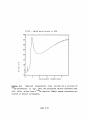
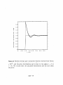
cases the Placzek expansion is not helpful. Figure 2.5 shows a
comparison between the numerical integration of the free particle
S(Q,o) (ideal gas formula) and equation (2.9.4) for a nucleus of mass
51
(vanadium) and scattering angle of 20'. Note that at this small
angle the expansion formula gives good agreement with the numerical
calculation: at larger angles such as 90' and 150° the agreement is
much worse, although in every case the high Q limit is the same. Figure
2.6 shows the numerical calculation for a mass 2 particle at two
tempertures. A pronounced temperature effect is seen. Moreover the
correction now has a clear hump at - 2 ~ - ' corresponding to the
derivative of the incident spectrum. Results such as this can only be
obtained by numerical integration.
Two computer programs exist
to perform
these numerical
integrations: PLACID calculates the Placzek correction for an ideal
gas, i.e. treating the particle as free. The other program is called
PLATOF and it allows the user to input a table of S(Q,o) values from a
separate calculation. Both programs can be made available for general
use if there is sufficient demand.
2.10
MERGING THE DATA TO FORM THE STRUCTURE FACTOR
Typically one will record the TDCS at several scattering angles in
a TOF diffraction experiment. On LAD there are currently 14 groups of
detectors, 7 on each side of the instrument. Which of these groups are
to be combined requires a decision by the experimentalist. A typical
approach might be as follows:
a) Correct each angle for inelasticity effects, particularly in the
self scattering.
b) Plot all the spectra on top of each other
page 2-21
c) For each group choose a range of Q values over which this
spectrum overlaps with at least one spectrum from a neighbouring group
at higher or lower scattering angle, and ignore those spectra which
clearly disagree with the others. Obviously this is a highly subjective
point in the analysis, but if all has gone well with the experiment it
should be fairly obvious where the overlaps occur. The object is to
avoid combining different detector banks where there are clearly
differences due to say not being able to perform the Placzek
correction accurately, such as occurs with light atoms such as
deuterium.
d) Merge the selected spectra over the selected Q range, using the
MERGE command, see section 3.12 and below.
e) Finally perform any remaining normalizations as needed such as
removing the incoherent scattering and dividing out the scattering
cross section. The result should either be in the units of differential
cross section (barns per steradian per atom/4n) or have dimensionless
units as a structure factor, S(Q).
The merging of spectra is achieved by weighting each spectrum with
the intensity with which it was measured. The weighting function is
obtained from the corrected intensity data of the vanadium sample
contained in the quantity
where the suffix j is used to label the jtth group of detectors. Hence
if C.(Qe) is the measured differential cross section for the jtth
J
group, the merged differential cross section is obtained by forming the
sum
page 2-22
This is achieved with the MERGE command, section 3.12
2.11
ANALYSIS TO PAIR CORRELATION FUNCTION
The inversion of the S(Q) data to pair correlation function, g(r),
i.e. inversion of equation 1.3.2, can be done by trivial Fourier
transform. Routines GTOS and STOG (see section 3.13) are available to
do this, and will allow the inclusion of a window or modification
function if needed.
However such direct Fourier transforms will inevitably lead to
spurious structure in the calculated distribution due to the finite
extent and statistical noise present in the data. This has been the
subject of a number of reports, including a preliminary one from the
Rutherford Appleton Laboratory by Soper [21], which was presented at
the ICANS-X meeting in October 1988. In this new method it is proposed
with increasing r to those that
to limit the fluctuations in r(g(r)-1)
are compatible with the observed width of the peaks in S(Q). In this
way the noise and truncation of the data are not reproduced in the
simulated pair correlation functions, at the same time that excellent
fits to the measured data are obtained. At the time of writing a full
account of this technique has still to be prepared for publication, and
the program, called MCGOFR, is not in a particularly user friendly
form, so at presemt it must be run under careful supervision. Even so
it is fully intended to make this program generally available to anyone
interested in using it. The basic philosophy of the approach is
described in Appendix C, which is a reproduction of the ICANS paper in
full.
page 2-23
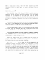
T I T L E : Total hard sphere cross section
6
I
I
I
I
I
-
4-
2-
08-
-
6-
-
4-
-
20-
scattering hard sphere cs
-
8-
-
6
0.4
0
I
I
I
I
I
1
2
3
4
5
Wavelength ( A )
Figure 2.1 Calculated scattering and total cross section for a hard
sphere fluid of density
= 0.5, with u=3.142. The fluid is assumed
to have unit scattering cross section per atom, and the capture cross
section is 0.4 at 1.8A. The crosses correspond to a structureless fluid
page 2-24
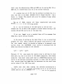
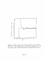
T I T L E : Sm148 perchlorate in D20
0
1
2
3
4
5
wavelength (Angstroms)
2.2
Measured transmission cross section for a solution of
148~m-perchlorate in D 2 0 Note the pronounced neutron resonance near
X=IA which arises from a 14'sm
impurity. Higher energy resonances are
Figure
visible at shorter wavelengths.
page 2-25
/
/
N(x) INCIDENT
NEUTRONS
'
/
Figure
2.3
Geometry
of
/
transmission problem for an arbitrary shaped
sample
page 2-26
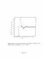
T I T L E : Placzek correction for vanadium at 20 deg.
Figure 2.4 Calculated TOF recoil correction (l+P) for a free vanadium
nucleus at two temperatures: 20K and 300K, and at a scattering angle of
20'. Note the large temperature effect at small Q values.
page 2-27
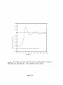
TITLE : Vanadium Placzek correction at 20 deg.
DOTS: NUMERICAL INTEGRATION
LINE: EGELSTAFF'S FORMULA
0
n
0.95
I
0
1
S
1
2
(
3
8
1
1
4
1
5
1
(
6
1
1
7
,
1
,
8
1
,
9
10
Q (Angstrom**-1)
Figure 2.5 Comparison of numerical calculation of recoil correction for
a vanadium nucleus at T=300K and scattering angle 20°, with Egelstaffts
approximate formula, equation (2.9.4), which does not have the correct
spectral dependence at small Q. Even so it gives good agreement at all
Q values
page 2-28
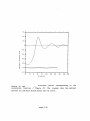
TITLE :
Placzek correction for deuterium at 20 deg.
Figure 2.6 Recoil correction for a free deuterium atom at 20K and 300K.
The scattering angle is 20°. Note again the large temperature effect at
small Q, and that a pronounced structure appears due to the substantial
energy transfers that take place in the scattering process,
page 2-29
.
SECTION 3
HOW TO RUN THE PROCEDURES
page 3-1
3.1 THE ISIS COMPUTING SYSTEM
3.1.1
The computers
The current ISIS computing system (sometimes referred to as PUNCH Pulsed Neutron Computer Heirarchy) is illustrated below and is fully
described in the PUNCH User Manual.
Terminal
Cambridge Ring
LAD FEM
(R55
vVAX
Ethernet
VAX8650
JANET
HUB Computer
Each instrument is controlled by a Front End Mini (FEM) computer
which in the case of LAD is a Micro-VAX 2. The central mainframe,
referred to as the HUB, is a VAX8650.
The FEM and the HUB are connected by two network systems - the
Cambridge Ring and Ethernet. The HUB is also the node for other wide
area networks such as JANET, for UK universities, and DECnet, EARN and
BITNET for world-wide access.
Users will be assigned their own username on the HUB (see Local
Contact for details) for use in analysing data. The username will be of
the form ABCOl where the letters are the initials of the user and the
numerals take into account several users with the same initials. The
same username may also be used to log on to the LAD FEM.
page 3-2
3.1.2
Getting started
>>>Note : any command typed into the computer should be followed by
pressing the RETURN key (sometimes referred to as Carriage Return CR).
This will be assumed throughout the manual.
To log on to the HUB
...
1. Press the BREAK key on the terminal until the prompt
DNS:
appears
2. Type CALL HUB
3. Press RETURN to make the prompt Username: appear
4. Type the username (eg ABCO1)
5. In response to the prompt Password: type password
6. A short command routine will then be executed, setting the
system ready for analysing LAD data, and then the user will be logged
on to the HUB and able to commence data analysis. The command routine
must be setup by the Local Contact during the first use of the
username.
Periodically the user will be required to change the password. This
is done by use of the command SET PASS.
Once logged on, the user ABCOl will have access to an area of disk
space for storing files in the directory [ABCOl] and any
sub-directories of it. In these areas there are full access rights ie
read,write,execute,delete. The user has limited rights usually read
only to areas within [LADMGR]. Initially, when the data is collected,
it is stored in the directory [LADMGR.DATA] on the FEM and
automatically transferred to the HUB in the same directory. However,
due to space restrictions the data is archived onto optical disk and
deleted within a few days. Data files are restored by issuing the
command RESTLAD when logged onto the HUB. This restores the raw data
page 3-3
files to the area [LADMGR.RESTORE], with the restore process taking a
maximum of about 10 minutes. The data files are held in this area for a
period of 3 days. Both these areas can be referred to by the logical
name 'inst-data' - for example a directory listing can be obtained by
DIR inst-data.
Programs and command files are stored in the area [LADMGR.PROGS]
which has the logical name 'g-f'. (Note: a 'logical namet is simply a
convenient synonym used to stand for a string of characters)
The user may wish to make use of sub-directories to help organise
the files within his own area. In this case the following commands are
useful:
CREATE/DIR [ABCOl.ANA]
-
create a sub-directory named [ABCOl.ANA]
SET DEF [ABCOl.ANA]
-
set the default directory to be
[ABCOl.ANA].
This has the effect that
subsequently the computer will assume
that a file is in the directory
[ABCOl.ANA] unless another directory is
specified.
SH DEF
- show the default directory.
3.2
DATA FILES AND BATCH SYSTEM
3.2.1
Data File Structure
The data on the FEM can be in 3 locations - the DAE, the CRPT or
disk (either as a .SAV file or a .RAW file). On the HUB it is either
.SAV or .RAW.
The convention used to name files involves 3 parts : a filename, an
page 3-4
extension and a version number. For data the filename is constructed
from the instrument name (3 characters) and a 5 digit run number. The
type of file is specified by the extension - for example SAV or RAW.
The full name of the raw data file (version 1) for run 1234 for example
In our programs we continue to use this form of
is LAD01234.RAW;l
nomenclature so that data for a specific sample can be recognised by
its run number and the type of data by the extension name. Within the
programs the instrument name and leading zeros in a run number need not
.
be specified.
In all the above cases the file structure is the same. There is a
header section which contains information supplied by the instrument
control program (ICP) on the FEM.
There are sections on :
-instrument parameters; for example detector angles, flight
paths, spectrum numbers for detectors and monitors.
-run parameters; for example date/time of start and end, number
of protons, neutrons and frames.
-sample parameters; for example title of run, dimensions.
These are followed by arrays containing :
-time of flight which is stored as the time boundaries for the
channels as specified by the ICP.
-each spectrum as counts per channel.
Files are in binary format but ASCII versions of parts of the data can
be provided.
The GENIE program can also create files in binary format but with a
different layout. The file starts with a selection of parameters from
the RAW data header section such as scattering angle and flight paths
and is followed by arrays containing the values of x, y and error on y.
Such binary files will be used extensively by our programs with the
page 3-5
type of data denoted by the extension.
Programs are available for converting these binary files to ASCII
format.
3.2.2
Batch System
The batch system enables a program to be run non-interactively so
as not to tie up the terminal. It is of most use for long programs,
such as those used to calculate the absorption correction and the
multiple scattering correction. Some useful batch related commands are
as follows;
SUBMIT VAN01234.COM
- submit the command file VAN01234.COM to
be run by batch.
SHOW QUE *$BATCH
- show the status of all batch queues.
DELETE/ENTRY=999 RLDESBATCH - delete batch job 999 (the entry number
999 may be obtained by use of the SHOW
QUE command) from queue RLDESBATCH (for
example).
SHOW SYS/BAT
-
shows all the batch jobs currently
executing in the current processor and
how much CPU time each has used. Note
that if a job has been submitted to a
different CPU from the current one the
amount of time in that job can only be
obtained by logging on to the appropriate
CPU. This is not normally possible for
HRPD, POLARIS and CRISP unless you know
the password because these FEM's have
limits on who can log on.
page 3-6
3.3 INSTRUMENT INFORMATION
3.3.1
Calibration
On a time-of-flight instrument the data must be converted from
stored counts in channels to counts in other units such as wavelength,
d-spacing and Q-vector. These conversions are determined by
standard equations :
X
where
2d sine
=
t
A
L
X
28
d
two
(Braggts equation)
is the time of flight
is the origin in time determined by the electronics
is the total flight path equal to the sum of the initial (I1)
and final (I2) flight paths
is the wavelength
is the scattering angle
is the d-spacing of the powder. peak
These parameters are determined with calibration experiments of two
types. The first equation can be used with neutron absorption
resonances which occur at fixed energy or wavelength. By measuring many
resonances from different foils placed in the incident beam, values for
A and L can be determined. Most resonances occur at high energies
(-eV) (short times-of-flight) so these calibrations give good values
for A.
The second equation of course leads to the familiar calibration
using standard powders such as Ni, A1203 and MgO. These experiments
will give values of A and the product Lsine. At short times there are
either no Bragg peaks or they cannot be resolved so that the value of A
by this technique is not as reliable as that from resonances.
As pointed out in Appendix A the Bragg peaks have an asymmetric
page 3-7
shape which varies with scattering angle, so the peaks have to be
analysed to take this into account.
The instrument calibrations are carried out by the Instrument
Scientists and do not normally need to be repeated by the user.
Nonetheless it is wise to look for discrepencies between the results
from different scattering angles to determine if the supplied
calibration is correct. The header sections of the .RAW data files
should contain the correct values. On the FEM they are stored in a file
called DETECTOR.DAT. If that file does not contain all the values or if
they need changing a similar file can be created on the HUB to be used
by our programs.
3.3.2
Spectrum numbering
All detectors and monitors are allocated a spectrum number. The
physical detectors are mapped to spectrum numbers by software via a
file called SPECTRA.DAT. These can be changed by the user at the start
of an experiment, but in most cases a standard setup is used. The
number of spectra and the number of channels per spectrum are defined
on the FEM by the ICP and their product defines the storage capacity
required and the maximum value is determined by the hardware in the
FEM
.
In the data analysis programs the spectra can be further combined
for example according to scattering angle. This will in general be
neccessary to reduce the volume of data and is particularly true for
the scintillator modules which have a large number of detector
elements. Subsequently a combined spectrum from several detectors is
treated as though being at the average angle. In the case of LAD the
detectors occur in groups at scattering angles of approximately 5O,
lo0, 20°, 35O, 58O, 90° and 150° and the default way of combining the
detectors is based on these groups.
Two of the spectra are always the monitors - one in the incident
beam and the second in the transmitted beam.
page 3-8
The header section of the data files also keeps a record of the
spectrum numbering and in our programs we make use of this data so that
the user does not need to know them.
3.3.3
Time channels
The time channel structure is set up by the ICP and three basic
structures are available : channel width constant with time, channel
width proportional to time-of-flight and width proportional to the
square of the time-of-flight. There can be up to five ranges of
time-of-flight each with a choice of structure.
The constant channel width is the simplest but has the disadvantage
that on converting to Q the data becomes squashed into the low Q region
with the high Q region having widely spaced points. The second choice
has the advantage that the channel widths are proportional to the
resolution over the whole range since the resolution is constant in
At/t and AQ/Q. For this option the distribution of points in Q is still
on constant increment but not as bad as the first option. The last
choice would provide constant increments in Q.
On LAD we have chosen the second option - that is the channel width
is proportional to time-of-flight. There is only one region staring at
200 us ending at 19500 us just before the next pulse which arrives at
20 ms. The constant of proportionality is 0.002 which allows for about
ten points across a Bragg peak at the backward angle (150°), highest
resolution detectors. Since the resolution worsens as the scattering
angle decreases and the constant does not change with angle, the number
of points at the lower angles are higher than necessary.
The combination of unequal Q increments and the increments in
general being smaller than neccessary for liquid and amorphous work
means that rebinning of data in Q is always required.
page 3-9
TABLE 3.1
Example of DETECTOR.DAT file
LAD February 1989
Number of
84 5
Det Delta
14.4
24.4
34.4
44.4
54.4
6 4.4
74.4
84.4
94.6
104.6
115.4
12 5.4
13 -0.7
14 -0.95
15-1.0
16-1.0
17-1.0
18 -1.0
19-1.0
20 -1.0
21-1.0
22 -1.0
23 -1.0
24-1.0
25 -1.0
26 -1.0
27 -1.0
28 -1.0
29 -1.0
30 -1.0
31 -1.0
32-1.0
33 -1.0
34 -1.0
35 -1.0
36 -1.0
37 -1.0
38 -1.0
39 -1.0
40 -1.0
41 -1.0
42 -1.0
43 -1.0
44 -1.0
detectors, Number of user table parameterddetector
Len2
1.128
1.128
1.128
1.128
1.128
1.128
1.128
1.128
1.047
1.047
1.033
1.033
-1.092
1.260
1.039
1.039
1.039
1.039
1.039
1.039
1.039
1.039
1.039
1.046
1.046
1.046
1.046
1.046
1.046
1.046
1.046
1.046
1.043
1.043
1.043
1.043
1.043
1.043
1.043
1.043
1.043
1.04
1.04
1.04
Code 2theta utl
150 145.6 1.0
150 145.6 1.0
150 145.6 1.0
150 145.6 1.0
150 145.6 1.0
150 145.6 1.0
150 145.6 1.0
150 145.6 1.0
150 9.6
1.0
1.0
150 9.6
1.0
150 4.8
1.0
150 4.8
150 180.0 2.0
2.0
150 0.01
2.0
150 88.4
150 88.8 2.0
2.0
150 89.1
2.0
150 89.5
2.0
150 89.7
150 90.0 2.0
2.0
150 90.3
150 90.55 2.0
2.0
150 90.9
150 57.0
2.0
150 57.2
2.0
150 57.45 2.0
2.0
150 57.8
150 58.0
2.0
2.0
150 58.3
150 58.7
2.0
150 59.0
2.0
150 59.3
2.0
2.0
150 34.1
2.0
150 34.4
2.0
150 34.7
2.0
150 34.9
2.0
150 35.3
2.0
150 35.6
2.0
150 35.9
2.0
150 36.1
150 36.4
2.0
150 19.1
2.0
2.0
150 19.5
2.0
150 19.8
ut2
1.25
1.25
1.25
1.25
1.25
1.25
1.25
1.25
1.25
1.25
1.25
1.25
0.00244
0.00244
1.25
1.25
1.25
1.25
1.25
1.25
1.25
1.25
1.25
1.25
1.25
1.25
1.25
1.25
1.25
1.25
1.25
1.25
1.25
1.25
1.25
1.25
1.25
1.25
1.25
1.25
1.25
1.25
1.25
1.25
page 3-10
ut3
10.0
10.0
10.0
10.0
10.0
10.0
10.0
10.0
10.0
10.0
10.0
10.0
44.0
44.0
1.0
1.0
1.0
1.0
1.0
1.0
1.0
1.0
1.0
1.0
1.0
1.0
1.0
1.0
1.0
1.0
1.0
1.0
1.0
1.0
1.0
1.0
1.0
1.0
1.0
1.0
1.0
1.0
1.0
1.0
ut4
0.006
0.006
0.006
0.006
0.006
0.006
0.006
0.006
0.016
0.016
0.02
0.02
0.001
0.001
0.014
0.014
0.014
0.014
0.014
0.014
0.014
0.014
0.014
0.008
0.008
0.008
0.008
0.008
0.008
0.008
0.008
0.008
0.012
0.012
0.012
0.012
0.012
0.012
0.012
0.012
0.012
0.013
0.013
0.013
ut5
0.
0.
0.
0.
0.
0.
0.
0.
0.
0.
0.
0.
0.
0.
0.
0.
0.
0.
0.
0.
0.
0.
0.
0.
0.
0.
0.
0.
0.
0.
0.
0.
0.
0.
0.
0.
0.
0.
0.
0.
0.
0.
0.
0.
*q18ua~a~em
01 uo;szaAuoD 1;un 30 sasodznd
aql 303 7 01 las aq ue3 z1 uaqt sa1;3 elep aql 30 uorlsas
za~ameledaql u; pau;gap IOU sr 1 31
*rnO*O130 an1eA 1eu;mou
1
aql aq 01 uayel s 1
6ZT+
sau;mzaIap
uo;1elq;1e3
aqA
aleds
51n
uo;ln1osa~
91"
X3uap;jja lo13alap ale1nqe3 01 sla~arnezed
€ln pue z1n
zo1e11~1~;3s=z
se8=1 apo3 ad& zo13alap
11"
: aze ase3 s;ql u; pue pau;gap zasn ale gn-1ln slalarnezed
aq1 !(avq ST 05 ) luarnnzlsu; aql sau;jap apo3 !a~oqepaugap se
ale elaqlz pue ~ ~ e l ~!laqmnu
ap
zolaalap aq1 s; urnnIo3 1 s ~ ;a q~j
'0
'0
'0
'0
'0
'0
'0
'0
'0
'0
'0
'0
'0
'0
'0
'0
'0
'0
'0
'0
'0
'0
'0
'0
'0
'0
'0
'0
'0
'0
'0
'0
'0
'0
'0
'0
'0
'0
'0
'0
Z
0'1
0'1
0'1
0'1
0'1
0'1
0'1
0'1
0'1
0'1
0'1
0'1
0'1
0'1
0'1
0.1
0'1
0'1
0'1
0'1
0'1
0'1
0'1
0'1
0'1
0'1
0'1
0'1
0'1
0'1
0'1
0'1
0'1
0'1
0'1
0'1
0'1
0'1
0'1
0'1
910'0
910'0
910'0
910'0
910'0
910'0
910'0
910'0
910'0
800'0
800'0
800'0
800'0
800'0
800'0
800'0
800'0
800'0
Z10'0
z10-0
210'0
Z10'0
Z10'0
210'0
Z10'0
ZTO'O
210'0
€10'0
€10'0
€10'0
€10'0
€10'0
€10'0
€10'0
€10'0
€10'0
€10'0
€10'0
€10'0
€10'0
sz-1
52'1
5
5
5Z'1
52'1
52'1
52.1
5
5
SZ.1
52.1
5
SZ.1
52'1
5
52'1
52'1
SZ.1
5
52.1
5 1
52'1
52'1
5
52'1
52'1
52'1
52'1
52.1
5
52.1
52'1
5
SZ.1
52'1
52'1
52'1
5
52'1
O'Z
O'Z
O'Z
O'Z
0'2
0.2
0'2
0'2
0'2
0'2
0'2
0'2
O'Z
O'Z
O'Z
O'Z
0'2
0'2
0'2
0'2
0'2
0'2
0'2
O'Z
O'Z
0.1
0'2
0'2
O'Z
0'2
0'2
0'2
0'2
0'2
O'Z
0'2
O'Z
0'2
0'2
0-2
6'06
55'06
E '06
0'06
L ' 68
5'68
1'68
8-88
9'88
E ' 65
0'65
L '85
E'85
0 ' 85
8'L5
59'LS
Z'L5
O'LS
9'9E
1'9E
6'SE
9'SE
E'SE
6'9E
L"7E
9*9€
1 *9€
Z'1Z
0'12
L'OZ
9'0Z
1 '02
8 ' 61
5'61
1'61
Z'1Z
0'12
L'OZ
9 'OZ
1 '02
3.4 OVERVIEW OF GENIE
For more details of this program the user should consult the GENIE
Manual. We will restrict ourselves to comments on the general
principles and the more important points in its operation.
The overall program structure is command driven, not by menu.
However where possible the individual routines called by the commands
will include a menu or question/answer structure for ease of use.
Workspaces are used for data manipulation. The number of workspaces
and their size (array length) can be chosen by the user. However there
is a limited memory space available so the product of the number of
workspaces and their length must be within this limit. There must
always be enough space for the graphics area and buffer areas. This
will normally be set for you.
Command files can be used for repetitive operations and can also
include terminal input. A command file is program run within GENIE
which executes commands from a .COM file instead of the user typing in
at the keyboard. Command files are run in GENIE by typing @ followed by
the name of the .COM file which is to be run. The name must be prefixed
by a directory name if the command file does not reside in the current
default directory.
There is an initialisation command file that is automatically read
on entering GENIE. This sets up values for the number of spectra and
their size and the default disk directories.
The data in Workspaces can be written to binary files for
subsequent reading back into workspaces.
External programs can be run to manipulate data in workspaces these are the FUNCTION and TRANSFORM commands and are used in our
programs for example to read in corrections parameters. Data in
non-GENIE type files (usually ASCII) can be read into workspaces using
page 3-12
the Load command.
The units of x in the workspace can be changed provided that the
workspace contains instrument parameters which are input via the SET
PAR command. The y-values of the data in the workspaces are stored in
the form of 'per unit of x' eg per microsec or per A-l. Care must be
taken when changing units and dividing - for example the correct order
is to change unit then divide. The option of scaling x to the y-unit
can be removed with the SET Yunit command.
3.4.1
Simple Example of GENIE commands
In order to read in a sample and vanadium spectrum, divide and
display as S(Q) the following operations are necessary :
>ASS 1234
>Wl=Sl
>Set PAR 1 10 1. 150. 0 0
>U/Q W1
>ASS 1235
>W2=S1
>Set PAR 2 10 1. 150. 0 0
>U/Q W2
>W3=Wl/W2
> D W3
>L/X 0 20
>D/E
3.4.2
assign run number for sample
read spectrum 1 into workspace 1
set parameters
change units to Q
assign run number for vanadium
divide S by V to give S(Q)
display S(Q)
change range of X (ie Q)
display new Q range and with error bars
GENIE command files
Operations can be stored as a command file and such a file is
provided for calculating the 'crude1 S(Q), i.e. (sample-can)/vanadium,
with no other corrections. The routine is started in GENIE with the
command @g-f:SQRAW, that is, the command file is called SQRAW.COM in
directory g-f. It prompts for sample, can and vanadium run numbers and
page 3-13
for the angle. The resulting "raw" S(Q) is displayed.
3.5 OVERVIEW OF PROGRAMS
The package provides a series of stand-alone Programs and GENIE
routines which are to be run in a particular order :
Program NORM normalises RAW data and produces output files with
extensions .MON and .NRM.
TRANSMISSION
Routines
calculate cross-sections from the
transmission data with extension .MON and creates files with extension
MUT
. .
Program CORAL calculates the corrections using the files with
extension .MUT and produces corrections files with extensions .ABS,
.MUL or .REF.
Routine VANSM treats the reference or vanadium spectra using files
with extensions .NRM and .REF and creates files with extension .SMO.
Routine ANALYSE takes the files with extensions .NRM, .ABS, .MUL
and .SMO to produce the corrected S(Q) at each angle as an output file
with extension .DCS.
Routine PLATOM calculates the self scattering at each angle,
creating an output file with extension .SLF. Routine INTERFERE
subtracts the self scattering in the .SLF file from the total
scattering in the .DCS file to yield the interference scattering which
is placed in a file of extension .INT.
Routine MERGE combines the individual angles in a file with
extension INT or DCS to produce a single S(Q) in a file with extension
.SOQ
.
page 3-14