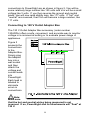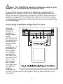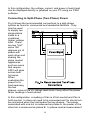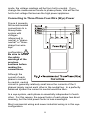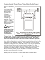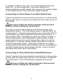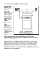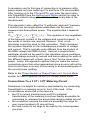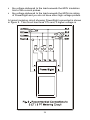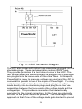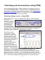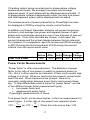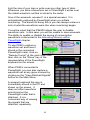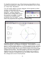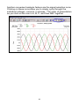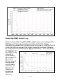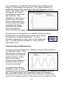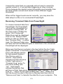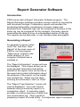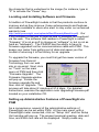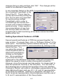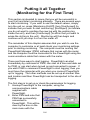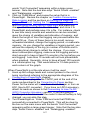
1
User’s Manual for PowerSight PS4000 Summit Technology, Inc. Walnut Creek, CA 94597 Tel: 1-925-944-1212 Fax: 1-925-944-7126 [email protected] http://www.powersight.com Rev for FW 3.3D / SW 3.4H Copyright 2012 by Summit Technology PowerSight is a registered trademark of Summit Technology, Inc. The PowerSight model PS4000 is designed to comply with part 15, subpart B, of the FCC Rules for a Class A digital device. Model PS4000 is manufactured by Summit Technology, Inc in the U.S.A. The standard warranty period is 12 months from date of purchase. We encourage you to advise us of any defects of design or manufacture of any of our products. We are dedicated to your successful use of the product. There are no user serviceable parts in your PowerSight meter. Opening the case voids your warranty and may result in present or future danger to users of the meter. The rechargeable battery inside is a custom-designed battery pack that is only to be replaced by authorized Summit Technology technical service personnel. Cleaning is to be done by use of a dry or damp piece of cloth. Grease may be removed by light application of isopropyl (rubbing) alcohol. Avoid the use of solvents, since they may dissolve or weaken the plastic enclosure. Do not use water or other conductive liquids since they may pose a safety risk. Use of this equipment in a manner not specified by Summit Technology can result in injury and voiding of warranty. Table of Contents Introducing PowerSight ............................................................. 7 Connecting to PowerSight ......................................................... 8 Voltage Test Leads ....................................................................................... 8 Current Probes .............................................................................................. 9 Connections to PowerSight ....................................................................... 11 Introduction to Power Delivery Configurations ........................................ 13 Connecting to Single-phase Power .......................................................... 15 Connecting to 120 V Outlet Adapter Box ................................................. 16 Connecting to Multiple Single-phase Loads ............................................ 17 Connecting to Split-Phase (Two-Phase) Power ..................................... 18 Connecting to Three-Phase Four-Wire (Wye) Power ............................ 19 Connecting to Three-Phase Three-Wire (Delta) Power ........................ 20 Connecting to Three-Phase Four-Wire Delta Power ............................. 21 Connecting to Three-Phase Grounded Delta Power ............................. 21 Connections Using 2 Current Approach .................................................. 22 Connections To a 3 CT / 3 PT Metering Circuit ...................................... 23 Connections To a 2 CT / 2 PT Metering Circuit ...................................... 26 Connections To an Open Delta (3CT / 2PT) Metering Circuit .............. 27 Connecting to Line-To-DC (LDC) Converter Accessory........................ 27 Measuring Multiple Parallel Conductors .................................................. 29 Measuring Currents Below the Range of the Current Probe ................ 31 Turning PowerSight On............................................................ 32 Connecting to Power .................................................................................. 32 Turning PowerSight On .............................................................................. 33 Turning PowerSight Off .............................................................................. 33 Checking out Connections Using PowerSight ....................... 34 Importance of Checking Connections and Wiring .................................. 34 Checking Voltage Levels – Using Checkout Connections .................... 36 Check Voltage Phase Sequence – Using Checkout Connections ....... 37 Checking Current Levels – Using Checkout Connections .................... 38 Checking I Phase Sequence – Using Checkout Connections .............. 39 Checking Phase Lag Angle - Using Checkout Connections ................. 40 Checking out Connections using PSM ................................... 41 Checking Voltage Levels – Using PSM ................................................... 41 Check Voltage Phase Sequence – Using PSM ...................................... 42 Checking Current Levels – Using PSM.................................................... 43 Checking I Phase Sequence – Using PSM ............................................. 43 Checking Phase Lag Angle – Using PSM ............................................... 44 Measurement Types ................................................................. 45 Voltage Measurements .............................................................................. 45 Voltage Measurements in PowerSight ..................................................... 47 Voltage Measurements in PSM................................................................. 48 Current Measurements .............................................................................. 50 Current Measurements in PowerSight ..................................................... 51 Current Measurements in PSM ................................................................. 53 Power Measurements ................................................................................. 54 Power Measurements in PowerSight ....................................................... 55 Power Measurements in PSM ................................................................... 56 Power Factor Measurements .................................................................... 57 True Power Factor Measurements in PowerSight ................................. 59 Displacement P.F. and Phase Measurements in PowerSight .............. 61 Power Factor and Phase Measurements in PSM .................................. 63 Energy Measurements ............................................................................... 64 Energy Measurements in PowerSight ...................................................... 65 Energy Measurements in PSM ................................................................. 65 Cost Measurements .................................................................................... 66 Cost Measurements in PowerSight .......................................................... 67 Cost Measurements in PSM ...................................................................... 68 Demand Period Measurements ................................................................ 68 Demand Period Measurements in PowerSight ....................................... 69 Demand Period Measurements in PSM .................................................. 69 Frequency Measurements ......................................................................... 70 Frequency Measurements in PowerSight................................................ 70 Frequency Measurements in PSM ........................................................... 71 Duty Cycle / Power Cycle Measurements ............................................... 72 Duty Cycle / Power Cycle Measurements in PowerSight...................... 72 Time and Capacity Measurements ........................................................... 73 Time and Capacity Measurements in PowerSight ................................. 75 Time and Capacity Measurements in PSM ............................................. 76 Harmonic Measurements ........................................................................... 76 Harmonic Measurements in PowerSight ................................................. 78 Harmonic Measurements in PSM ............................................................. 78 Swells (Surges) and Inrush Measurements ............................................ 79 Dips (Sags) Measurement ......................................................................... 80 High-Speed Transient Measurements ..................................................... 80 Measurement Modes ................................................................ 82 Introducing Measurement Modes ............................................................. 82 Phase-Neutral vs Phase-Phase vs 2 Current Mode .............................. 82 Changing the Voltage Measurement Mode in PowerSight ................... 84 Changing the Voltage Measurement Mode in PSM ............................... 84 50/60/400Hz vs DC vs Variable Frequency ............................................ 85 Changing the Frequency Measurement Mode in PowerSight .............. 86 Changing the Frequency Measurement Mode in PSM.......................... 87 Always Positive Power versus Negative Power Allowed ...................... 87 Changing the Power Measurement Mode in PowerSight ..................... 88 Changing the Power Measurement Mode in PSM ................................. 89 Defining Inputs ............................................................................................. 89 Changing Input Ratios in PowerSight ...................................................... 91 4 Changing Input Ratios in PSM .................................................................. 91 Voltage & Current Waveforms ................................................. 93 Introduction................................................................................................... 93 Saving Consumption Waveforms.............................................................. 93 Receiving Stored Consumption Waveforms ........................................... 95 Viewing Consumption Waveforms ............................................................ 95 Monitoring Power Consumption............................................ 100 Introduction................................................................................................. 100 Basic Consumption Data Logging .......................................................... 101 Receiving Consumption Data Log from PowerSight ............................ 104 Viewing Consumption Logs ..................................................................... 105 Custom Consumption Data Logging..................................... 107 Introduction................................................................................................. 107 Starting Data Logging ............................................................................... 107 Stopping Data Logging ............................................................................. 108 Setting the Consumption Logging Period .............................................. 109 Setting Measurement Types .................................................................... 109 Setting Measurement Modes................................................................... 111 Saving and Retrieving Data Setups to File or PowerSight.................. 111 Monitoring Swell/Dip/Inrush .................................................. 113 Introduction................................................................................................. 113 Swell/Dip Event Log .................................................................................. 114 Swell/Dip RMS Graph Log ....................................................................... 116 Swell/Dip Event Waveforms .................................................................... 117 Setting the Swell/Dip Trigger Thresholds in PowerSight ..................... 117 Setting the Swell/Dip Trigger Thresholds in PSM ................................ 119 Receiving Swell/Dip Data from PowerSight .......................................... 120 Viewing Swell/Dip Event Data ................................................................. 122 Monitoring High-speed Transient Events ............................. 123 Introduction................................................................................................. 123 Transient Event Log .................................................................................. 124 Transient Event Waveforms .................................................................... 125 Setting the Transient Trigger Thresholds in PowerSight ..................... 126 Setting the Transient Trigger Thresholds in PSM ................................ 127 Receiving Transient Data from PowerSight .......................................... 129 Viewing Transient Event Data ................................................................. 130 Allocating Memory within PowerSight .................................. 132 Report Generator Software .................................................... 134 Introduction................................................................................................. 134 Generating a Report ................................................................................. 134 Viewing a Report ....................................................................................... 136 Other Functions of PowerSight ............................................. 138 Calibrating PowerSight ............................................................................. 138 Setup Functions ......................................................................................... 138 Administrative Functions .......................................................................... 139 5 Other Functions within PSM .................................................. 143 Introduction................................................................................................. 143 Remote Control of PowerSight ................................................................ 143 Locating and Installing Software and Firmware .................................... 144 Setting up Administrative Features of PowerSight via PSM ............... 144 Setting Operational Features of PSM .................................................... 145 Putting it all Together (Monitoring for the First Time) ......... 146 Working with Graphs and Waveforms .................................. 149 General....................................................................................................... 149 Reading Graphs and Waveforms ........................................................ 151 Zooming and Panning ............................................................................ 153 Troubleshooting & Frequently Asked Questions (FAQ) ...... 156 Advanced Motor Diagnostics Option .................................... 160 Introduction .............................................................................................. 160 Capturing On-Line Motor Data ............................................................. 160 Frequency Analysis Option ................................................... 162 Overview of the Keypad Functions ....................................... 163 Compatibility Guide................................................................ 165 Specifications* ........................................................................ 167 6 Introducing PowerSight Congratulations on your decision to buy a PowerSight 4000! You have just purchased one of the smallest and yet most powerful instruments for measuring and analyzing electric power that exists. The PS4000 is a complete solution for the measurement and analysis of all aspects of power: ♦ High-speed transient analysis ♦ Swell/Dip analysis ♦ Harmonics analysis ♦ Demand analysis ♦ Data logging ♦ Automated report writing ♦ Wiring and system analysis The philosophy of the product is to give you an instrument that answers your questions about electric power in a truly convenient size at an attractive price. If you are looking for a simple yet powerful tool that can be easily and reliably installed and operated, one that provides for comprehensive data analysis, you've found your tool of first choice. Whether your interest is in ♦ The quality of incoming power, ♦ Managing power consumption, or ♦ Maintaining and comparing equipment PowerSight puts all the power in the palm of your hand! *Note: Throughout this manual, whenever we refer to an individual key of the keypad, we print the name on the key enclosed by square brackets. For example, the “Volt” key is referred to as [Volt]. 7 Connecting to PowerSight Voltage Test Leads A Deluxe Voltage Probe set consisting of four leads is included with each PowerSight. Each of the voltage test leads is 6 feet (2 meters) long, with safety banana jacks at one end and safety plunger clamps at the other end. Each is labeled at both ends as the Va, Vb, Vc, or Vn test lead. The safety plunger clamps have telescoping jaws that you can actuate while keeping your fingers three inches away from the actual metallic contact. Regular test probes have conventional alligator jaw attachments that require your fingers to be within one inch of the metallic contact. Also, the method of attaching them can allow a gap in the insulation between the lead and where they join. This is where your thumb and finger are pressing while you actuate it. For these reasons, to avoid unnecessary risk of shock, regular voltage test leads should not be connected to or disconnected from live circuits and should definitely not be connected to or disconnected from voltages above 120 Vrms. Another word of caution: Whenever connecting to a live circuit, remember that the jaws of a voltage test lead are much wider when they are open than when they are closed. The potential to short two adjacent terminals or wires is a constant danger when connecting to a live circuit. Depending on the current capacity of the circuit being shorted, a deadly explosion of molten material can result! Once they are securely connected, the deluxe voltage leads are safe for steady voltages of the 600 Vrms rating of PowerSight. The clamps of the deluxe voltage leads are rated for 1000V working voltage, measurement category II. This is equivalent to measurement category III for a working voltage of 600V, the rating of PowerSight. 8 Summit Technology also sells a fused voltage lead set (order DFV). The safety advantage of fused leads is that if there is a short through the insulation of a lead to ground, the fuse in the handle should quickly blow out, preventing the lead from vaporizing in an explosion of molten metal. The safety disadvantage of fused leads occurs when the fuse is blown or is removed. The user will measure 0 volts on a live circuit and may be tempted to lower his safety awareness, possibly resulting in shock or damage. The DFV probes are rated for 1000V, measurement category III. Current Probes Summit Technology provides a variety of probes for your use. They offer different measurement ranges, different sizes and physical characteristics, and the ability to measure different types of current. Probes such as the HA1000 are excellent choices to use with PowerSight because they support all the accuracy specifications of the product. For instance, the HA1000 has an accuracy of 0.5% whereas many probes on the market have an accuracy of 23%. Also, the HA1000 maintains its accuracy for frequencies up to 20,000 Hz. With our spectrum analyzer option (order FAO) it can be used to measure frequencies up to 100,000 Hz riding on the power line. This allows accurate current and power readings of distorted waveforms, accurate readings of harmonics, and the measurement of current transients that other probes would not even detect. Phase shift is also an important probe characteristic. The HA1000 has less than 1/2 degree of phase shift across the frequency range when measuring currents above 50 amps and just 1.5 degrees at 5 amps. This means that instantaneous measurements of power are highly accurate, regardless of the waveform shape. The phase shift characteristics of most other probes on the market are not this good. This results in erroneous power and cost measurements and distorted waveforms. Please Note: To diminish phase shift when measuring small currents, it is advisable to clamp onto multiple "turns" of the same conductor in order to increase the effective current being sensed. 9 The HA5 offers two advantages over the HA1000, but these advantages come at a cost. Its advantages are that the HA5 is a very small size (5.25 × 2.00 × 1.35 inches) and second, it offers much greater sensitivity since it reads currents from 20 milliamps to 5 amps (as compared to the HA1000 measuring 1 - 1,000 amps). The tradeoff is accuracy. The probe has a basic accuracy of 2% and its phase shift varies by frequency and by amplitude. All told, you can expect to measure current to a nominal 2.25% accuracy and power and cost to a nominal 3% accuracy using the HA5 probe. The HA100 probe is the same compact size as the HA5. The HA100 measures from 0.1 to 100 amps at 2% accuracy. It is a good choice over the HA1000 if you wish to lock PowerSight, its leads, and current probes inside a power panel that you are monitoring. It is also a good choice when small size is important while measuring currents above 5 amps. The HA100 is a popular choice for a second set of probes. For very large currents and large bus bars, we offer the HA3000, the FX3000, and FX5000. The HA3000 is capable of clamping onto cables of up to 2.50 inches wide and bus bars of 1.97 × 5.31 inches or 2.56 × 3.94 inches. It offers linearity of ±0.5% ±1.5 amps from 5 to 3000 amps. The HA3000 offers added safety to users who clamp over bare bus bar since the user's hands do not pass close to the exposed bus bar. It is available as a special order item. The FX3000 and FX5000 are "flex" type probes. They consist of a tube about 0.55 inch in diameter and 24 inches long. The ends of this tube can snap together around a conductor to measure current. Flex probes are very handy when space is tight, when multiple cables must be clamped around, or when connecting around an unusual bus bar that the HA3000 cannot fit over. They are also lighter and less expensive. The flexible tube creates a circle with an inside diameter of 7 inches. This circle can be deformed into various shapes to accomplish your measurement goals. The basic accuracy of the flex probes is good, measuring from 10 to 3000 amps within 1% accuracy. However, readings can vary as much as 2% depending on the position of the flex 10 probe while connected. Position the flexible portion of the probe around the conductor so that the cable from the probe drops straight down and the head rests against the conductor and is at a right angle with the conductor. The frequency response of flex probes is very good, but phase shift increases with frequency. Unlike other manufacturers’ flex probes, ours do not require batteries for them to run. You must use added caution when connecting an FX series current probe around exposed conductors and bus bars since you must pull the tube around the conductor and thus get your hands and arms closer to it than when using HA series clamp-on type current probes. Wise practice dictates that you use high insulation protection on hands and forearms in these circumstances or deactivate the circuit. The DC600 probe is used for AC current measurements from 5 to 400 amps and DC measurements from 5 to 600 amps. It offers accuracy of 2% ±1 amp from 5 - 400 amps and 3% accuracy for DC from 400-600 amps. This probe relies on Hall effect technology and its output varies slightly over time. Therefore, a zero level adjustment is provided on the probe's handle for initial zeroing before each measurement session. The probe accepts one cable up to 1.18 inch diameter or two cables of up to 0.95" diameter. Unlike other manufacturers’ DC probes, ours do not require batteries for them to run. New probes and adapters are being introduced regularly, so if you have a special need, give us a call. Please Note: Always inspect the metal surfaces of clamp-on probes before use. Clean them with a rag or sand them with fine sand paper and then slightly oil the surface. Any dirt or rust will affect the accuracy of the measurements! Connections to PowerSight Voltage test leads plug into the back end of PowerSight. Each test lead of the Deluxe Voltage Test Lead set is labeled (Vn, Va, Vb, or Vc) and each jack is similarly labeled (Vn, Va, Vb, or Vc). 11 Note: The Vn test lead is a different color from the other leads (black). Similarly, the Vn jack on PowerSight is a different color from the other ones (black). Connecting anything other than neutral or ground to the Vn jack can jeopardize your safety, the functioning of the unit, and the accuracy of the unit. Current probes plug into the sides of PowerSight. Each current probe is labeled (Ia, Ib, Ic, or In) and each jack is similarly labeled (Ia, Ib, Ic, or In). The Ia and In probes plug into the left side of the unit. The Ib and Ic probes plug into the right side of the unit. When plugging a current probe into PowerSight, the flat side of the plug should be faced upwards so the label is readable. This will align it properly for plugging into the PowerSight case. Clamp-on probes have a correct orientation in which to attach them. On most probes' head, there will be an arrow pointing in the direction of the conductor being measured. When clamped onto Ia, Ib, or Ic, the arrow should point along the conductor from the power source towards the load. If the current probe is connected backwards, its waveform will appear upside-down when you upload waveforms, it may be slightly less accurate in its current readings, and, most importantly, if you operate in positive/negative power measurement mode, power readings will be disastrously wrong. 12 Introduction to Power Delivery Configurations Figure 1 presents most common power delivery configurations. PowerSight is able to measure voltage, current, power, power factor, and more for all of these systems. Figure 1A presents the normal single-phase and two-phase service as found in a residential service. In North America, Van and Vbn are 120V and are 180 degrees out of phase with each other. When heavier loads are encountered, Vab (240V) is used by delivering both hot voltages to the load. Neutral provides the current return path. If the load is balanced, there will be relatively little neutral current. Refer to figures 2, 3, 4, and 5 for various ways to connect to single-phase and two-phase power service. Figure 1B presents normal three-phase “wye” power service. Voltages are usually measured from phase-to-neutral. Neutral provides the current return path. If the load is balanced, there will be relatively little neutral current. Refer to figure 6 for how to connect to a three-phase wye power service. Figure 1C presents normal three-phase delta service. Voltages are usually measured from phase-to-phase. In North America, service is usually supplied as 120V, 240V, 480V, 600V, 4160V, or 12,500V. In most of the world, service is usually supplied as 381V, 5,716V, or 11,431V. Summit Technology has voltage 13 probes for direct connect to all of these services. Refer to figure 7 for how to connect to a delta power service. When there is no access to measuring one of the currents, figure 8 presents the 2 current approach for measuring power. This approach is also useful for measurement of an open delta circuit as described in Connections to an Open Delta Circuit (2PT/3CT)figure 10. Although phase-to-phase is the normal voltage measurement mode for this service, PowerSight can be set to phase-to-neutral (even though the neutral is not connected). In this case, the measured voltages will be phase-to-metering-neutral (such as Van= 277V for a 480V service) and all other measurements will also be correct. Figure 1D presents three-phase four-wire delta service. In this configuration, a neutral is supplied from a point midway between two phases. This is handy when 240V delta is supplied. Vbn and Vcn supply conventional 120V single-phase power and Van provides 208V, if needed. In this configuration, depending on what you are measuring, you may choose to measure in phase-tophase mode or in phase-to-neutral mode. Figure 1E presents grounded delta service. This configuration is actually not very common. It can be attractive to use if an electrically isolated three-wire delta service is available and there is a need to provide the power a long distance away at a private facility (such as a saw mill). By grounding one of the phases at the source, the cost of supplying one of the phases to the remote site is saved. A motor at that site would be connected to phase A, phase B, and earth ground. There is increased danger in this configuration over normal isolated delta service since the reference to ground is intentionally an excellent conductive path. Nevertheless, PowerSight will provide the desired measurements in this configuration. 14 Connecting to Single-phase Power Figure 2 presents the basic connections to a single-phase system. Be sure to follow the safety warnings of the previous sections before making the connections. Clamp your A phase current probe onto the "Hot" wire. Make a metallic connection to neutral with the Vn voltage lead. Similarly connect the Va lead to "Hot". Since voltage now comes into PowerSight on Va and current is sensed by Ia, the power and power factor for this single-phase system will be available as phase A power and phase A power factor. Caution: Until you are certain that your voltage connections to PowerSight are correct, disconnect any current probes. This is because PowerSight and all of its connections float at the potential of Vn. If Vn is "hot", there may be a breakdown through the insulation of any attached probes. Helpful Hint: How to Identify the "Neutral" lead. Normal single-phase wiring follows the convention of "neutral" being the white wire, "hot" being the black wire, "hot2" being the red wire, and "ground" being the green wire. If the wiring and your 15 connections to PowerSight are as shown in figure 2, Van will be some relatively large number like 120 volts and Vcn will be a small voltage like 3 volts. If you then reverse the ground and neutral leads, Van will now read slightly less, like 117 volts. If "hot" and "neutral" are reversed, then Vcn will become a large number, like 117 volts. Connecting to 120 V Outlet Adapter Box The 120 V Outlet Adapter Box accessory (order number 120ADPa) offers a safe, convenient, and accurate way to monitor voltage in a commercial setting or to evaluate power usage of appliances. Figure 3 presents the connections to the Adapter Box. Simply plug the adapter box into a wall socket and then attach the voltage and current leads into PowerSight. Each lead is labeled to eliminate errors in connections. Note: Make sure that the hot and neutral wiring being measured is not reversed. If so, PowerSight and its attachments will "float" at 120 V. 16 Note: The 120ADPa is rated for continuous duty of up to 15 Arms. Do not exceed this continuous load. To evaluate the power usage of an appliance, simply plug the appliance into the top of the 120 V Outlet Adapter Box after the other connections have been made and verified. Even without an appliance plugged in, the adapter box offers a convenient means of checking for transients or analyzing the harmonic content of the incoming voltage. Connecting to Multiple Single-phase Loads Figure 4 presents a means to monitor 3 single-phase loads simultaneously. The loads must all share the same neutral voltage connection. If the loads run off the same line voltage, connect Va, Vb, and Vc to the same "hot" wire. Ia, Ib, and Ic serve the 3 loads. This approach can also be used to evaluate the current of a 4th load, but the power used by that load will not be calculated. 17 In this configuration, the voltage, current, and power of each load can be displayed directly or graphed on your PC using our PSM software. Connecting to Split-Phase (Two-Phase) Power Fig 5 shows the recommended connections to a split-phase system as found in commercial and residential facilities. They may be used to supply two single phase loads or a combined higher voltage load. There are two "Hot" wires 180 degrees out of phase with each other and sharing the same neutral. Appliances such as ovens that require 240V will span across both hot wires. When evaluating the power for a load spanning the two phases, remove the VN voltage lead since it may affect the power factor readings of each phase. In this configuration, a reading of Van is of hot-neutral and Vbn is hot2-neutral. In does not need to be connected and Vn should not be connected when the load spans the two phases. The power associated with one hot is measured as phase A, the power of the other hot is measured as phase B. In phase-neutral measurement 18 mode, the voltage readings will be from hot-to-neutral. If you change the measurement mode to phase-phase, Vab will be the hot-to-hot voltage that serves the high power appliance. Connecting to Three-Phase Four-Wire (Wye) Power Figure 6 presents the recommended connections to a three-phase system with voltages referenced to neutral, a "phaseneutral" or “threephase four-wire wye” configuration. Be sure to follow the safety warnings of the previous sections before making the connections. Although the current of each phase is carried by neutral, neutral current is generally relatively small since the currents of the 3 phases largely cancel each other in the neutral leg. In a perfectly balanced system the current in neutral would be zero. In a wye system, each phase is essentially independent of each other. For this reason, the power factor of each phase has direct meaning, but the total power factor is less meaningful. Most commercial wiring and newer industrial wiring is in this wye configuration. 19 Connecting to Three-Phase Three-Wire (Delta) Power Figure 7 presents the recommended connections to a three-phase system with voltages referenced to each other instead of to neutral. This is a "delta", "phasephase", or “threephase three-wire” configuration. Be sure to follow the safety warnings of the previous sections before making the connections. Please Note: Do not connect the Vn input to anything when measuring in phase-phase measurement mode. This may affect the measurements associated with individual phases. In a delta configuration, current flowing in each phase is due to the interaction of 2 different voltages. For instance Ia current is the resultant of Vab and Vca. Normally, there is no way to determine what portion of the current is due to which voltage. For this reason, only the total power and total power factor have definite meaning in a delta system. However, comparing the power factors of each phase can be valuable for spotting a connection problem or problem with the load. Delta power is common in motors and older industrial sites. 20 A variation of delta is “four-wire” (or “center-tapped”) delta (see figure 1D). In this configuration, if the main interest is in measuring phase-neutral voltage, then connect the neutral voltage to the neutral input for more accurate voltage readings Connecting to Three-Phase Four-Wire Delta Power Figure 6 presents the recommended connections to a three-phase delta system where a neutral is provided from the center of one of the phases. Be sure to follow the safety warnings of the previous sections before making the connections. This type of system allows delivery of both three-phase and single-phase power. The three-phase power is typically 240V for running motors. The dual single-phase power is typically 120V for running lights and small equipment, from one power service. It also provides 208V. Depending on what you intend to monitor, it may be appropriate to set PowerSight in phase-phase voltage measurement mode (to monitor three-phase loads or to look at total power) or in phase-neutral voltage measurement mode (to monitor single phase loads). Although the selection of voltage measurement mode affects what voltage levels are displayed and recorded (phase-phase versus phase-neutral), it does not affect the power and power factor calculations. Connecting to Three-Phase Grounded Delta Power Figure 7 presents the recommended connections to a three-phase system with one phase tied to ground. No connection is made to the neutral input. One of the phases originates from ground. Be sure to follow the safety warnings of the previous sections before making the connections. 21 Connections Using 2 Current Approach In the previous sections, the approach used to measure power has been based on determining the power of each phase and then summing them to get the total power. The 2 current approach (figure 8) allows you to determine the total power from measuring only 2 of the 3 currents and combining them with the 3 voltages of the three-phase circuit. The disadvantage of this approach is that you cannot determine the power, power factor, or VA of each individual phase and, of course, you cannot record the current of one of the active phases. One motivation for using this type of connection is to save time and money. By only connecting to 2 of the 3 currents, a small amount of time can be saved. The frugal user appreciates this approach because he can save the cost of one current probe when buying a system in order to measure total power. Another motivation occurs in situations where one of the phases cannot be measured due to accessibility. . 22 A necessary use for this type of connection is to measure utility power where only two metering CTs and three PTs are provided. After hooking up to the CTs and PTs, you enter the input ratios into PowerSight (see the Setting Input Ratios section) in order to record the correct values (the values on the primary side of the transformers). This approach is also called the “2 wattmeter approach” because it mimics how two single-phase wattmeters can be used to measure total three-phase power. The equation that it depends on is: Wtotal = (Vab × I a ) + (Vcb × I c ) . This equation is true regardless ∑ ∑ of the harmonic content of the voltages and currents present. A few words of caution are required, however. First, a voltohmmeter cannot be used for this calculation. That is because the equation depends on the instantaneous products of voltage and current. That is normally quite different from the product of the RMS voltage and RMS current. Second, a single-phase wattmeter should not be used for this calculation since conditions normally change second by second and hence adding the watts of two different setups will, at best, give a “feel” for the correct true power. Lastly, this approach requires that you make the correct connections more than other approaches since an error will not be obvious and there is no way of recovering to an educated guess of the correct power reading. Refer to the Phase-Neutral vs Phase-Phase vs 2 Current Mode section for how to operate the unit in 2 current probe mode. Connections To a 3 CT / 3 PT Metering Circuit Sometimes it is helpful to monitor a load indirectly, by connecting PowerSight to a metering circuit in front of the load. A few circumstances where this is the case are: the CTs (current transformers) and PTs (potential transformers) of the metering circuit are readily accessible for connecting to, whereas the actual load carrying cables are not the conductors carrying the load are physically too large for your current probes to fit around them the load current is too large to be read by the current probes you have 23 the voltage delivered to the load exceeds the 600V insulation limit of the current probes the voltage delivered to the load exceeds the 600Vrms rating of PowerSight and you do not have other high voltage probes. A typical metering circuit showing PowerSight connected is shown in figure 9. This circuit has three CTs and, if higher voltage is 24 present, may have three PTs. It is typical for metering a threephase four-wire wye type service. The currents flowing to the load are considered the “primary currents”. Those currents are “stepped down” by each CT to a “secondary current” according to the ratio of the CT printed on its rating plate. A typical value would be 600:5 (120:1). The output of each CT must have some burden across it for the secondary current to flow. The current probes of PowerSight are clamped around the secondary of each CT. Make sure to use current probes that are suited for accurate measurement in the 0-5 amp range. The HA5 is best for this. The HA1000 or HA100 may be acceptable, depending on the current level. Once the current probes are attached, it is best to set the input ratios for each of the current probes (see the Setting Input Ratios section). This will allow the displayed values and logged values to reflect the primary current level instead of the secondary current level. This in turn allows accurate power and cost readings without having to multiply the results times some ratio. Remember that these ratios are reset to 1:1 whenever PowerSight is turned off. Similarly, the PTs take a primary voltage and step it down to a secondary value. If the primary voltage is below 600Vrms, you will not need to hook up to the PTs (in fact, there will probably be none present). The ratio of the stepping down of the voltage will be printed on the rating plate of the PT. Typically this would be 2400:120 (20:1). As with the CTs, this ratio should be entered into PowerSight (see the Setting Input Ratios section) to simplify interpreting the results. 25 Connections To a 2 CT / 2 PT Metering Circuit Figure 10 shows recommended connections to a metering circuit with only 2 CTs or 2 PTs. This type of metering circuit may be preferable when cost is an issue (less instrument transformers are used) or when metering a delta service with no reference to neutral. The discussion of the previous section (Connection s To a 3 CT / 3 PT Metering Circuit) applies to this circuit as well, with one important exception. If you clamp onto the CTs, rather than clamping onto each of the primary currents directly, PowerSight must be operating in the 2 Current Probe mode of operation (see the Phase-Neutral vs Phase-Phase vs 2 Current Mode section). 26 Connections To an Open Delta (3CT / 2PT) Metering Circuit In the open delta configuration, two PTs and 3 CTs are available. Make the voltage connections as shown in figure 10 of the Connections to a 2CT / 2PT Metering Circuit section. For current connections, connect the A and C phase probes as shown in figure 10 and attach the B phase current probe to the B phase CT. You will not need to operate in the 2 Current Probe mode of power measurement since there are 3 currents being monitored. Connecting to Line-To-DC (LDC) Converter Accessory The Line-To-DC Converter accessory (order number LDC4) converts the voltage that is being monitored into DC voltage to run and charge PowerSight. The applications of this option are: Electrical room monitoring where a 120V outlet jack is not available for your charger Monitoring where an extension cord from a 120V outlet jack would be a safety hazard Monitoring on a rooftop, power pole, or power pad Reliable charging for the PS4000 when there is concern that an available 120V outlet jack may be switched off by other personnel Simplified monitoring connections (no need to think about powering PowerSight when installed inside a CASW weatherresistant case. Figure 11 shows the correct method of connecting the LDC to PowerSight. The LDC comes with two long red input leads that end with a stackable safety banana plugs. These stackable plugs are to be inserted directly into two of the inputs of PowerSight. If you are monitoring power without a neutral, we recommend plugging them into the Va and Vb inputs. If an external neutral is present, we recommend plugging them into the Va and Vn inputs. In any case, there needs to be a potential between them of at least 100 Vrms and no more than 500 Vrms from 50 Hz or 60 Hz power. 27 The LDC also comes with in-line fuse assemblies plugged into the stackable plugs. These red assemblies contain 1000V fuses. They provide protection if a short should occur in the LDC. The two voltage leads that would normally be plugged into PowerSight are plugged into the loose ends of the in-line fuses. At this point, PowerSight is ready to measure voltages as usual and the LDC is connected in parallel to two of the inputs of PowerSight. You may wish to remove the in-line fuse assemblies, plug your voltage leads directly into the stackable plugs, and plug the in-line fuse assemblies between the loose ends of the voltage leads and the voltage clips. This provides a connection that is electrically equivalent to the normal connection, but the fuses are physically as close to the power source as possible. The advantage of this approach is that if one of the voltage leads gets shorted to ground 28 (perhaps from being cut by a panel door), a fuse quickly blows, providing added protection. Note: Do not use the LDC without the in-line fuses being connected between it and the power source. The fuses are the only circuit protection for the LDC. When the input side of the LDC is fully connected properly, plug the long DC output plug into the DC input jack of PowerSight. The red charging indicator near the jack will light up if everything is operating and connected properly. Note: If a fuse is burned out or missing, it will appear that there is no voltage at the source. Verify that the fuses are working properly before assuming that the source is dead. Injury may occur if you wrongly assume that the source is deactivated. Measuring Multiple Parallel Conductors A common problem with measuring large currents arises when the current of each phase is carried by several parallel conductors. For instance the A phase current may be carried in 4 parallel conductors, as are the B and C phases, resulting in 12 conductors to measure. In this case, the work-around is to clamp onto just one of the conductors of each phase and enter an input ratio to record the correct total current of each phase. A fast way of doing this is to enter an input ratio of 4 : 1 for each phase in the example of 4 parallel conductors. This may offer adequate accuracy for your needs. However, experience shows that although the current in each conductor of the same phase is similar in size, they are typically NOT identical. Overcoming the problem of unequal currents in parallel cables takes a few steps to do it accurately. 29 1. Put a different probe on each conductor of a given phase and then viewing the currents of each probe simultaneously (see the Checking Current Levels – Using Checkout Connections section). 2. Start monitoring for 10 seconds or so and then stop monitoring (see the Starting Data Logging and Stopping Data Logging sections). 3. Press the [Current] key and then the [More] key four times to view the average current for the A phase (which is actually just one of the conductors of one of the phases). Write it down. 4. Press the [Current] key and then the [More] key four times again to view the average current for the B phase. Write it down. 5. Repeat these actions in order to get the average current of each of the conductors for the same time period. 6. Find the total of the average currents of each of the conductors of the same phase. 7. Divide the total of the average currents into the average current of conductor you wish to connect to during the actual monitoring session. This yields the portion of the total current that flows through the conductor that will be measured. 8. Set the input ratio of the phase being measured to the number determined in the previous step. For instance if the total of the average currents was 1000 amps and the average current of the probe on the conductor you wish to use during the actual monitoring session had an average of 260 amps, then enter an input ratio for that phase of 1000 : 260 (or 1 : 0.26). 9. Perform steps 1 through 8 for each phase. 10. Now connect each probe to the chosen conductor of each phase and begin monitoring. All the readings and logged values will be substantially correct. 30 Measuring Currents Below the Range of the Current Probe A problem with measuring smaller currents arises when the current to be measured is below the range of the current probe. In such cases, the current may not be read or the reading may be inaccurate. In addition, any waveforms that are captured will have excessive noise on them. If you are using a flexible current probe, you can simply wrap it around the conductor twice in order to double the magnetic field strength. This can get it in the measurement range and it boosts the signal to noise ratio. If you use this method, set the input ratio for the current probe to 1 : 2 (see the Changing Input Ratios in PowerSight section). If the current to be measured is small, it may be acceptable to open the circuit and insert an extra length of wire that is wound up into a coil of 10 turns. Clamping your current probe around this extension coil will boost the signal strength 10 times and allow accurate reading of small currents. If you use this method, set the input ratio for the current probe to 1 : 10 (or however many turns there are in the coil). 31 Turning PowerSight On Connecting to Power Although PowerSight comes with Li-ion rechargeable batteries, those batteries are intended to keep PowerSight functioning during limited power failures and to allow quick measurements without the bother of always having to find a 120 Vrms source. When fully charged, the batteries can power the unit for up to 8 hours. For longer usage and to recharge the batteries, your unit has been supplied with a wall-mount power supply. This power supply cannot be used with the model PS3000 and the PS3000 power supply cannot be used with the PS4000. To use this power supply, simply plug it into any 120 Vrms source (use the model CHG4 charger for 120Vrms and the model CHG1 for 220V) and then plug its barrel-type plug into the 12 VDC input jack on the back end of PowerSight. If charging voltage is available, an LED indicating light will immediately shine through the small hole located to the left of the input jack. Allow 4 hours to fully charge the unit. If you wish to operate PowerSight without being tethered to a power outlet, the Line-to-DC converter accessory (order LDC4) offers the ability to power a PS4000 (or a PS250) directly off the line voltage being monitored. It works with 50 Hz and 60 Hz power, operating off 100 to 480 Vrms input, single-phase or threephase. All this versatility is obtained without setting switches or changing connections. The LDC4 is especially convenient when monitoring in areas where 120 V outlets are not readily available. If you need to operate the LDC4 off of 600V phase-to-phase service, connect one input to a hot phase and the other input to neutral. 32 The internal batteries are automatically charged when the wallmount supply is connected to the unit (or when PowerSight is connected to the LDC4 accessory). The internal batteries are not to be replaced by the user. Only batteries provided by Summit Technology are to be used in PowerSight. Turning PowerSight On Simply press the white push-button switch on the front panel and PowerSight will be operating (pressing the button again, turns the unit off). The message that the meter is performing a system test will appear for a few seconds and then the greeting will appear. You can change this greeting at any time by following the directions in the administrative functions that are accessed by pressing the [Admin] key. Please note that turning PowerSight on does not automatically start monitoring and logging. Refer to the Putting it all Together (Monitoring for the First Time) section for how to start monitoring and logging. Turning PowerSight Off To turn PowerSight off, simply press the white push-button switch on the front panel. This provides a graceful software/firmware shutdown. If pressing the button briefly does not turn the meter off, press and hold the push-button down for 3 seconds to force a hardware shutdown. If this is a recurring problem, contact [email protected]. 33 Checking out Connections Using PowerSight Importance of Checking Connections and Wiring After connecting to power, it is wise to check that everything is connected correctly and that the wiring of the facility is correct. There are two primary methods for doing this. You may either send waveforms from PowerSight to your PC and visually check that all connections are correct (Checking out Connections Using PSM), or you can use the "Checkout Connections" feature within PowerSight to quickly and easily do this. The importance of having all connections correct cannot be overstated. If connections are not correct, important decisions may be made based on erroneous data or monitoring sessions lasting several weeks may have to be repeated. Common connection errors and their negative results are: Current probe attached backwards. Normally, if current probes are attached backwards, PowerSight senses this and turns them around in software so you still get the correct power readings. This is one of the features that makes PowerSight easy to use. However, if you press the [Wave] key to save waveforms and a current probe is backwards, that current will appear upside down (180 degrees out of phase). More importantly, if PowerSight is in the Positive/Negative Power measurement mode, a backwards current probe will have a disastrous effect on the power, KWH, and cost readings (typically the display will present 1/3 of the correct value). Voltages and currents of same phase not matched. If the Va voltage probe is connected to Va, but the Ia current probe is attached to Ib or Ic, large errors will occur in measurement of power and power factor. For instance in a perfectly balanced system with .92 power factor and no harmonics, if the connections of the Ia and Ic probes are switched, the true power will fall 33% and the power factor of each phase will become 0.12, 0.92, and 0.80. 34 Current probe not fully connected to PowerSight. The current probe connector needs to be fully seated within its socket. If it is not, the reading may be 0 (resulting in a loss of about 1/3 of the power), the probe may be misidentified (resulting in current readings of a fraction or a multiple of the correct value), or the display may say “Ia input too large” and PowerSight will refuse respond to the keys of the keypad. To visually checkout if all connections are accurate, enter PSM (the PowerSight Monitor program) on your PC, connect to PowerSight, click on “Receive Waveforms” at the main menu, then click on “Snapshot” and then “Receive and View”. To use the Checkout Connections feature of PowerSight, press the [Setup] key and then press [Yes/Accept] to the question "Checkout Connections?" Checking out the connections requires making six observations or tests. These are: Check of Voltage Levels – compare size and level of all 3 voltages Check of Voltage Phase Sequence – review the order in which the voltage appear Check of Current Levels - compare size and level of all 3 phase currents and neutral Check of Current Phase Sequence – review the order in which the 3 phase currents appear Check of Phase Lag Angles – verify that the amount displacement phase angle between the voltage and current of each phase is a reasonable amount and that it is a similar amount for each phase. Once you have used the View Waveform feature of PSM or the Checkout Connections feature of PowerSight to verify that connections are correct, you can proceed with confidence knowing that the power wiring is correct and that PowerSight is connected to it properly. 35 Checking Voltage Levels – Using Checkout Connections After pressing [Yes/Accept] to the display "Checkout Connections?", you are asked "Checkout Voltage Levels?". If you press [Yes/Accept], then the voltages of all three phases are presented on the display and are updated each second. First check that the voltage measurement mode is correct. If the measurement mode is phaseneutral, all measurement labels take the form Vxn, where "n" stands for neutral and "x" is a, b, or c depending on which phase is being presented. If the measurement mode is phase-phase, labels take the form Vxy, where "xy" is ab, bc, or ca. Changing the measurement mode has a large effect on the size of the voltage readings. For instance, in a three-phase 120 volt phase-neutral (wye) system, the voltage measurements in phase-phase mode will be 208 volts ( 120 × 3 ). Similarly, a three-phase 480 volt phase-phase (delta) system will display 277 volts ( 480 / 3 ) if it is measured in phase-neutral mode. How to change the measurement mode is described in the Measurement Modes chapter. At this point, examine the voltage measurements to see if their size seems correct. In single-phase measurements, as described in the Connecting to Single-phase Power section, typically the measurement mode is phase-neutral. Hot-neutral is generally 120V in North America, 100V in Japan, and 230V everywhere else. Ground-neutral should be no more than a few volts. Larger ground-neutral readings probably mean that the neutral is under heavy load, there is a faulty neutral-ground bond, there is a high resistance neutral connection, or the ground wire is floating. If two "hot"s are connected, as in figure 3, you may wish to be in phase-phase measurement mode so that Vab reads 240V as is typically used for heavier residential loads in North America. In this case, Vbc and Vca should each read 120V. In a three-phase phase-neutral system, all three voltages should be roughly the same. Typical values in North America are 69, 120V, 208, 277, and 346V. When using 5KVP probes on a 4160V circuit, the typical value is 2400V. When using 15KVP probes on a 12,500V circuit, the typical value is 7200V. 36 In a three-phase phase-phase connection, all three voltages should be roughly the same. Typical values in North America are 120, 240, 480, 600, 4160 (using 5KVP probes or connected to PT secondaries while using input ratios), and 12,500V (using 15KVP probes or connected to PT secondaries while using input ratios). If one of the phases has a center tap midway through it and the center tap is connected to neutral, this is a "four-wire" or "centertap delta" service. Depending on the load being monitored, it may be best to measure a center-tap delta system in phase-neutral measurement mode. Typical readings on a 240V center-tapped delta service in phase-neutral measurement mode would be 120V on two of the phases and 208V on the third phase. The voltage readings of this test are updated each second. When the readings appear to be correct, press [Yes/Accept] to move on to the next test. Check Voltage Phase Sequence – Using Checkout Connections In a three-phase system, each of the three voltage phases is 120 degrees out of phase with the other two phases. This means that if one phase reaches its peak at one instant, the next phase will reach its peak 120 degrees later and the third phase will reach its peak 240 degrees after the first (the first will again reach its peak 360 degrees after its last peak). This provides for the smooth supply of three-phase power. Certain loads, such as motors, must have the voltages connected so that the peak voltages arrive in a certain sequence. If this sequence is reversed, the load will not work and damage may occur. Determining the voltage phase sequence is necessary before connecting such loads. Also, if voltage leads of PowerSight are not connected to the correct phases, the voltage readings will be mislabeled and the power readings will be incorrect. For these reasons, it is a good idea to check the phase sequence of the voltages before connecting loads or beginning monitoring. 37 To determine the phase sequence, press [Yes/Accept] when asked "Check V Phase Sequence?" The following display is typical: The order in which the voltages are listed is the order in which the peaks of the voltage arrive. Looking at the first phase letters, the example above shows a phase sequence of A-B-C, which is typical. If the displayed sequence is C-B-A, then it's likely that the voltage leads are connected incorrectly or that the phases are mislabeled. The numbers of the second line are the number of degrees between each phase. These numbers are updated each second. When the readings appear to be correct, press [Yes/Accept] to move on to the next test. Checking Current Levels – Using Checkout Connections Checking the current levels provides an instant view of whether the system is operating correctly and the current probes are attached correctly. To view all current levels at once, press [Yes/Accept] when asked "Checkout Current Levels?". The following display is typical: Generally, the 3 active phases should be similar in size and the neutral current should be relatively small. The readings are updated each second. Note: If one of the phases is 0 or extremely high, the plug of the current probe may not be pushed all the way into PowerSight. When the readings appear to be correct, press [Yes/Accept] to move on to the next test. 38 Checking I Phase Sequence – Using Checkout Connections In order to get correct power readings for each phase, voltages and currents of the same phase must be combined. The phase sequence for voltages was determined in an earlier test. Next we need to verify that the currents have the same phase sequence. To determine the current phase sequence, press [Yes/Accept] when asked "Check I Phase Sequence?". The following display is typical: The order in which the currents are listed is the order in which the peaks of the current arrive. Looking at the phase letters, the example above shows a phase sequence of A-B-C, which is typical. If the displayed sequence is C-B-A, then one or more current probes are either connected to the wrong phase or are connected backwards (unless the voltage phase sequence was also C-B-A). If the current phase sequence is correct, it does not automatically mean that the current probes are connected correctly. The phase angles between them and the phase lag between the voltage and current (the next test) must also be examined. The numbers of the second line are the approximate number of degrees between each phase. In a normal three-phase system, they should appear as 120 degrees ±15 degrees. If there is a large imbalance between the angles of the phases (like 62-22869), then one or more current probes are probably backwards. If one of the numbers is 0, then the current probes on either side of it are connected to the same phase. Also, even if the phase sequence and degrees are correct, the current probes may be connected to the wrong phases. For instance, if Ia is paired with Vb, Ib is paired with Vc, and Ic is paired with Va, the current sequence and phase angles will appear correct, but power readings for each phase will be incorrect. Note that in a single-phase system with two hot phases (a twophase system), the phase angle between them will be 180 degrees. Also note that in a four-wire delta system with most of 39 the loads operating phase-to-neutral, you may see normal operation of 90, 90, and 180 degrees between the currents. The sequence and phase angle numbers are updated each second. When the readings appear to be correct, press [Yes/Accept] to move on to the phase lag angle test. Checking Phase Lag Angle - Using Checkout Connections Current may lead or lag voltage by as much as 90 degrees. Typically current lags voltage or may slightly lead it. The Phase Lag Angle Test displays the approximate phase angle, also known as "displacement", between voltage and current for each phase. To determine the phase lag angle for each phase, press [Yes/Accept] when asked "Check Phase Lag Angles?" The following display is typical: The measurement is presented as the number of degrees that current lags voltage for each phase. If the current of a phase lags the voltage by 30 degrees, the display will show 30 degrees. If the current leads voltage by 7 degrees, it will be displayed as -7. In a three-phase connection, if all previous tests had acceptable results but this test reveals that one and only one of the phases has a phase lag of 0 or 180 degrees, then the current probes are matched with the wrong voltage phases. If all previous tests had acceptable results and none of the phases is 0 or 180 degrees, but this test reveals that one or more phases have lag angles of more than 90 degrees, then one or more current probes are connected backwards. Simply clamp the current probe on backwards for the phase that has a phase angle of greater than 90 degrees. The phase lag angle numbers are updated each second. When the readings appear to be correct or if you wish to perform all the tests over again, press [Yes/Accept] to move back to the first test. 40 Checking out Connections using PSM The PowerSight Manager (PSM) software is included in the cost of your PowerSight meter. You can use it to visually determine if the system connections and levels are correct. Use PowerSight’s Checkout Connections feature for a simple measurement-based approach to checking out the connections. Checking Voltage Levels – Using PSM At the main menu, click on “Receive Waveform”, then “Receive and View”. A waveset (a set of 7 time-coincident waveforms) will be transferred from PowerSight to PSM and then a dialogue box opens asking you to choose what signals to view. Make your primary choice “Voltage”, and your secondary choice “Set All”. Next click on “View”. Now that you are viewing the voltage waveforms, there are several questions that need to be answered. First of all, is the voltage measurement mode correct? If the measurement mode is phase-neutral, all measurement labels at the top will be Van, Vbn, and Vcn. The first letter after the “V” is the phase that is connected to and the "n" stands for neutral. If no neutral is connected to PowerSight, this measurement is in reference to the neutral point between all the phases that are connected. If the measurement mode is phasephase (as shown in the example), the labels will be Vab, Vbc, and Vca. Vab is the voltage potential between the A and B phases. 41 Changing the measurement mode has a large effect on the size of the voltage readings. For instance, in a three-phase 120 volt phase-neutral (wye) system, the voltage measurements in phasephase mode will be 208 volts ( 120 × 3 ). Similarly, a three-phase 480 volt phase-phase (delta) system will display 277 volts ( 480 / 3 ) if it is measured in phase-neutral mode. How to change the voltage measurement mode is described in the PhaseNeutral vs Phase-Phase vs 2 Current Mode section. Next, are the sizes of all three phases about the same (except when connected to a 4 wire delta while in phase-neutral measurement mode)? Are they the expected size? The RMS value of each waveform is listed in the heading of the graph (such as “Vab” in the example with “469.2” beneath it, indicating that Vab = 469.2 volts). Check Voltage Phase Sequence – Using PSM While still viewing all voltage waveforms of a three-phase system, notice in what order they reach their peak value. Normally, the order should be A-B-C. In other words the highest level of the Van (or Vab) waveform will be followed next by the highest level of the Vbn (or Vbc) waveform, which will be followed by the highest level of the Vcn (or Vca) waveform (see the example). An order of B-C-A or C-A-B is the same as an A-B-C sequence; the reference point just starts at a different place (for instance BC-A is just a portion of the continuing sequence of A-B-C-A-B-C). Sometimes an order of C-B-A is correct. Some utilities deliver power in that sequence and sometimes a motor will be connected 42 in that manner to make it spin “backwards”. An order of B-A-C or AC-B is the same as C-B-A, the reference point just starts in a different place (for instance B-A-C is a portion of the continuing sequence of C-B-A-C-B-A). Checking Current Levels – Using PSM Next click on the blue “Back Arrow” icon and select “Current”, “Set All”, and “View”. Now that you are viewing the current waveforms, there are several questions that need to be answered. First, are the sizes of each of the three phases reasonable (depending on the type of load, currents of each phase may be very similar or fairly different)? The RMS value of each waveform is listed in the heading of the graph (such as “Ia” with “136.5” beneath it, indicating that Ia=136.5 amps), similar to how they are presented for voltage as seen in the Checking Voltage Levels section. Also check the shapes of the current waveforms. Some of the more common current waveforms that may be seen are shown in the Checking Phase Lag – Using PSM section below. Checking I Phase Sequence – Using PSM While still viewing all current waveforms of a three-phase system, notice how they reach their peak value. Each of the peaks should be the same distance from each other (similar to as shown in the Checking Voltage Sequence – Using PSM section). This even spacing must continue across the screen. In a three-phase system there will be a constant 120 degrees apart (5.5 msec for 43 60 Hz, 6.3 msec for 50 Hz). If one or two of the current probes is backwards, the peaks will not be evenly spaced. If that is the case, determine which probe can be turned around to get the spacing correct. After turning it around and verifying that the spacing is now correct, determine in what order the currents reach their peaks. This sequence must be in the same order as was seen for the voltages. If they are not, swap two of the probes. This will correct the phase sequence. Verify once again that the spacing between them is still correct. If not, repeat the instructions of this section. Checking Phase Lag Angle – Using PSM When viewing the voltage and current waveform of a given phase, you will notice a timing relationship between the two waveforms (refer examples below). The point at which the current reaches its peak may lead or lag the peak of the voltage by as much as 90 degrees (90 degrees at 50 Hz is 4 msec, at 60 Hz it is 4.2 msec). Typically current either lags the voltage or it may slightly lead it. By the time you have gotten to this test, you have verified that the voltages and currents are reasonable sizes and that their sequences appear to be correct. Now select a view of “voltage and current” and “phase A” only. Check how much time passes between the peak of the voltage and the peak of the current. It must be within 90 degrees. Next select a view of “phase B” only and then “phase C” only. In each case, note the time delay between the peak voltage and the peak current. It should be close to the same. If one current leads voltage and the other two currents lag voltage by different amounts, then two of the voltage or current probes are probably switched. If the delays are the same for all phases, but they are more than 90 degrees, then the current probes are probably not matched to the correct voltages probes and will need to be moved without changing the phase sequence. 44 Measurement Types Voltage Measurements Voltage is the difference in electromotive potential between two points. Simply stated, it is the force that generates current flow and to measure voltage, two points of connection are required. In AC circuits, this force, measured in volts, usually varies continuously and always reverses direction. In DC circuits, it is usually steady and never reverses direction. If the voltage changes in a repeating fashion, then it is called a periodic function. All AC power distribution is based on voltage changing at a periodic rate. There are several key voltage measurements: Instantaneous voltage Peak voltage RMS voltage Voltage crest factor Maximum voltage Minimum voltage Average voltage Present voltage Voltage swell (surge) Voltage dip (sag) Voltage transient. The instantaneous voltage is simply the voltage present between two points at an instant of time. When the voltage is graphed over time, the graph is called the voltage waveform. The peak voltage, Vpk , is the instantaneous voltage of the greatest magnitude (either positive or negative) over a period of time. A measure that changes continuously is of limited use. A far more useful measurement is RMS voltage, wherein a single number is generated to describe a continuously varying voltage. The beauty of RMS voltage is that in power calculations, it makes a contribution to power roughly equivalent to a DC voltage of the same magnitude. RMS voltage is defined as the square root of 45 the mean of the square of the instantaneous voltage over one cycle of the fundamental frequency: Vrms = ∑v N 2 . When measuring DC volts the RMS value is the same as the DC value. Voltage crest factor is the ratio of peak voltage of a cycle over the RMS voltage of the same cycle. Vcf = Vpk / Vrms . A perfect sine wave has a crest factor of 1.414 ( 2 ). Maximum, minimum, and average voltage in power measurements refers to the maximum, minimum, and average of RMS voltage measurements during a time of interest. For the PS4000, the RMS of every full cycle is measured, so these numbers are exact. In the PS4000, the present voltage is the summary of the RMS voltage over one second. It is the average of the RMS voltages of every cycle during the most recent second. A voltage swell (or surge) is an RMS voltage that exceeds some trigger level. A voltage dip (or sag) is an RMS voltage that falls below some trigger level. In the PS4000, the trigger levels can be set to an actual voltage level or as a percent deviation from a normal voltage. The RMS calculations for determining swell and dip are performed every ½ cycle, so these measurements are exact. When we speak of a voltage transient, we are speaking of an instantaneous voltage that exceeds a trigger level. An absolute trigger level is an instantaneous level that includes the underlying periodic waveform. A relative trigger level is an instantaneous level that has the underlying periodic waveform removed. In the PS4000, trigger levels can be set for both relative and absolute voltage transient levels. 46 Voltage Measurements in PowerSight PowerSight performs all commonly desired voltage measurements. When in phase-neutral measurement mode, the RMS (root mean square) voltage between Vn and the Va, Vb, and Vc input jacks is displayed by simply pressing [Volt] repeatedly. The sequence of the display as [Volt] is pressed is Van > Vbn > Vcn. In the phase-phase measurement mode, Vab, Vbc, and Vca are displayed instead. If energy consumption is being monitored, the maximum, minimum, and average RMS voltage is displayed by repeatedly pressing [More...] after displaying the appropriate present voltage. In this way, by combining the [Volt] and [More...] keys, there are 12 RMS voltage measurements available. For instance, if the average voltage between Vb and Vn is desired, press: [Volt] (to display )Van, [Volt] (to display Vbn), [More...] (to display maximum Vbn), [More...] (to display minimum Vbn), and then [More...] (to display average Vbn). Note that if 47 PowerSight is not monitoring consumption, the maximum, minimum, and average values are the results from the last monitoring session. Please note that when PowerSight is operating in 2 current mode, Vca is not calculated or displayed and Vbc is presented as Vcb. To set PowerSight for reading phase-neutral, phase-phase, or DC voltages, refer to the Measurement Modes chapter. If a connection is not made to the Vn input, PowerSight will find the neutral point between all the phases in doing its phase-neutral measurements. Information about the largest swell, the lowest dip, the largest absolute transient, and the largest relative transient for both voltage and for current can be viewed on PowerSight. Just press the [Spikes] key repeatedly until the summary for the type of measurement appears (such as “Voltage Dips”). The summary tells how many events have occurred and what the trigger level is. Pressing the [More…] key repeatedly will tell the important information about the worst of that type of event: the magnitude, duration, and timestamp. The total harmonic distortion (THD) of voltages is displayed using the THD function, discussed later in this chapter. Voltage Measurements in PSM The consumption data log can record maximum, minimum, and average RMS voltage for each phase for each logging period. The summary values at the top of the screen are the maximum, minimum, and average of all the values shown on the screen. When viewing consumption waveforms, the average RMS of the cycles of the waveform is shown at the top, with the average crest factor listed below it. The instantaneous value of each point of the waveform can be determined using the vertical scale. If a harmonic analysis is displayed, the RMS voltage is also listed 48 When viewing voltage swell logs, the highest ½ cycle RMS level of each event is displayed. An event starts when the trigger is exceeded and ends either when 10 cycles have passed or when a ½ cycle does not exceed the trigger level (whichever is longer). Voltage dip logs display the lowest ½ cycle RMS level of each event. Each event starts with the trigger and ends in 10 cycles or when a ½ cycle does not fall below the trigger level (whichever is longer). When viewing swell/sag RMS graphs, the RMS of each ½ cycle is graphed and the most extreme measurement, with its timestamp, is presented at the top. When viewing transient waveforms, the instantaneous values of the voltage are graphed, as with consumption waveforms. But the summary value at the top is the Vpk value above the trigger, with its timestamp. If trending data is being recorded and PowerSight is operating in phase-neutral voltage measurement mode, the average Van, Vbn, and Vcn voltages for each second will be displayed and recorded each second. If in phase-phase voltage measurement mode, the average Vab, Vbc, and Vca voltages for each second will be displayed and recorded each second. The measurements of voltage presented on PowerSight can also be displayed in PSM by using the remote control feature. In addition our Report Generator software will present maximum, minimum, and average voltage of each phase during any one or two intervals of time set by the user. If two time intervals are chosen, it will report the percent change and the actual change between the two intervals. For instance, if a comparison report is chosen and Vab average is 480 V during the first interval and 478 V during the second interval, then the report would show: % Before After Units Change Change Voltage, A phase, Avg. 480 478 volts -2.0 -0.4% The total harmonic distortion (THD) of voltages is displayed using the THD function, discussed later in this chapter. 49 Current Measurements Current is the flow of charged particles, usually electrons, through a point. Current is measured in units of amps (which is short for amperes) and its symbol is commonly “I”. In AC circuits, current often varies continuously and always reverses direction. In DC circuits, it is usually steady and never reverses direction. If the current changes in a repeating fashion, then it is called a periodic function. There are several key current measurements: Instantaneous current Peak current RMS current Current crest factor Maximum current Minimum current Average current Present current Current inrush (swell or surge) Current dip (sag) Current transient. The instantaneous current is simply the current passing through a point at an instant of time. When the current is graphed over time, the graph is called the current waveform. The peak current, Ipk , is the highest instantaneous current over a period of time. A measure that changes continuously is of limited use. A far more useful measurement is RMS current, wherein a single number is generated to describe a continuously varying current. The beauty of RMS current is that in power calculations, it makes a contribution to power roughly equivalent to a DC current of the same magnitude. RMS current is defined as the square root of the mean of the square of the instantaneous current over one cycle of the fundamental frequency: Irms = ∑i N 2 . When measuring DC amps the RMS value is the same as the DC value. 50 Current crest factor is the ratio of peak current of a cycle over the RMS current of the same cycle. Icf = Ipk / Irms . A perfect sine wave has a crest factor of 1.414 ( 2 ). Maximum, minimum, and average current in power measurements refers to the maximum, minimum, and average of RMS current measurements during a time of interest. For the PS4000, the RMS of every full cycle is measured, so these numbers are exact. In the PS4000, the present current is the summary of the RMS current over one second. It is the average of the RMS currents of every cycle during the most recent second. A current inrush (or swell or surge) is an RMS current that exceeds some trigger level. A current dip (or sag) is an RMS current that falls below some trigger level. In the PS4000, the trigger levels can be set to an actual current level or as a percent deviation from a normal current. The RMS calculations for determining swell and dip are performed every ½ cycle, so these measurements are exact. When we speak of a current transient, we are speaking of an instantaneous current that exceeds a trigger level. An absolute trigger level is an instantaneous level that includes the underlying periodic waveform. A relative trigger level is an instantaneous level that has the underlying periodic waveform removed. In the PS4000, trigger levels can be set for both relative and absolute current transient levels. Current Measurements in PowerSight PowerSight performs all commonly desired measurements of current. The RMS (root mean square) currents of the A, B, and C phases and of the neutral line are available by simply pressing [Current] repeatedly. The sequence of the display is Ia > Ib > Ic > In. If energy consumption is being monitored, the maximum, minimum, and average RMS current is displayed by repeatedly pressing [More...] after displaying the appropriate present current. In this way, by combining the [Current ] and [More...] keys, there are 16 RMS current measurements available. 51 For instance, if the average current of the C Phase is desired, press: [Current] (to display Ia), [Current] (to display Ib), [Current] (to display Ic), [More...] (to display maximum Ic), [More...] (to display minimum Ic), and then [More...] (to display average Ic). Note that if PowerSight is not monitoring consumption, the maximum, minimum, and average values are the results from the last monitoring session. Note that when PowerSight is in 2 current mode, Ib is not measured or displayed. When measuring DC current, the RMS value is the same as the DC value. To set PowerSight for reading DC currents, refer to the section on Setting Measurement Modes. Remember that you need to have a DC current probe in order to read DC current. Information about the largest swell, the lowest dip, the largest absolute transient, and the largest relative transient for both voltage and for current can be viewed on PowerSight. Just press 52 the [Spikes] key repeatedly until the summary for the type of measurement appears (such as “Current Swells”). The summary tells how many events have occurred and what the trigger level is. Pressing the [More…] key repeatedly will tell the important information about the worst of that type of event: the magnitude, duration, and timestamp. The total harmonic distortion (THD) of currents is displayed using the THD function, discussed later in this chapter. Current Measurements in PSM The consumption data log can record maximum, minimum, and average RMS current for each phase for each logging period. The summary values at the top of the screen are the maximum, minimum, and average of all the values shown on the screen. When viewing consumption waveforms, the average RMS of the cycles of the waveform is shown at the top, with the average crest factor listed below it. The instantaneous value of each point of the waveform can be determined using the vertical scale. If a harmonic analysis is displayed, the RMS current is also listed. When viewing current inrush logs, the highest ½ cycle RMS level of each event is displayed. An event starts when the inrush trigger is exceeded and ends either when 10 cycles have passed or when a ½ cycle does not exceed the trigger level (whichever is longer). Current dip logs display the lowest ½ cycle RMS level of each event. Each event starts with the trigger and ends in 10 cycles or when a ½ cycle does not fall below the trigger level (whichever is longer). When viewing swell/sag RMS graphs, the RMS of each ½ cycle is graphed and the most extreme measurement, with its timestamp, is presented at the top. When viewing transient waveforms, the instantaneous values of the current are graphed, as with consumption waveforms. But the summary value at the top is the Ipk value above the trigger, with its timestamp. 53 If trending data is being recorded and PowerSight is operating in phase-neutral voltage measurement mode, the average RMS current of each phase and neutral for each second will be displayed and recorded each second. If in phase-phase voltage measurement mode, the average RMS current of each phase for each second will be displayed and recorded each second. The measurements of current presented on PowerSight can also be displayed in PSM by using the remote control feature. In addition, our Report Generator software will present maximum, minimum, and average current of each phase and neutral during any one or two intervals of time set by the user. If two time intervals are chosen, it will report the percent change and the actual change between the two intervals. For instance, if a comparison report is chosen and Ia average is 48.0 A during the first interval and 47.8 A during the second interval, then the report would show: % Before After Units Change Change Current, A phase, Avg. 48.0 47.8 amps -0.2 -0.4% The total harmonic distortion (THD) and K factor of currents is displayed using the THD function, discussed later in this chapter. Power Measurements There are three basic interrelated measurements of power: True power Apparent power Reactive power Apparent power is defined as the sum of the products of the RMS currents and their associated RMS voltages: Papp = VA = (Vanrms × Iarms ) + (Vbnrms × Ibrms ) + (Vcnrms × Icrms ) . In other words, if you measure the RMS voltage (measured in volts) and the RMS current (measured in amps) and multiply them together, you get the apparent power (measured in VA). 54 True power is more complicated. It is defined as the average of the sum of the products of the instantaneous currents and their associated instantaneous voltages over one or more cycles: ∑ (v × i ) ∑ (vbn × ib ) + ∑ (vcn × ic ) . Ptrue = Watts = an a + N N N True power equals apparent power when there is no phase lag in the load and no harmonics are present, otherwise it is less than the apparent power. This is why an ammeter cannot be used to accurately measure true power in most industrial circuits. Reactive power is the square root of the difference between the squares of the apparent power and the true power: = Pvar VAR = ( Papp − Ptrue ) . 2 2 When the fundamental voltages and currents are in phase and no harmonic currents are present, reactive power is zero. Peak demand of the demand period is an important measurement that is covered in the Demand Period Measurements section. Power Measurements in PowerSight PowerSight performs all commonly desired power measurements. Total true power (watts or KW), total reactive power (VAR or KVAR), and total apparent power (VA or KVA) measurements are available by simply pressing [Power] repeatedly. The sequence of the display is KW > KVAR > KVA. If energy consumption is being monitored, the maximum, minimum, and average power is displayed by repeatedly pressing [More...] after displaying the appropriate power type. In this way, by combining the [Power] and [More...] keys, there are 12 power measurements available. 55 For instance, if the maximum reactive power is desired, press: [Power] (to display watts), [Power] (to display VAR), and then [More...] (to display maximum reactive power). Power Measurements in PSM The consumption data log can record maximum, minimum, and average true power and apparent power for each phase for each logging period. In addition is can record the maximum, minimum, and average true or apparent total power. When graphed, the VAR can be displayed. The summary values at the top of the screen are the maximum, minimum, and average of all the values shown on the screen. When viewing consumption waveforms, the average true power of the cycles of the waveforms are shown at the top right (if both voltage and current were recorded. If all phases are displayed, only the total true power is displayed at the top right. If a harmonic analysis of a phase is displayed, the true power of that phase is also displayed. 56 If trending data is being recorded and in phase-phase voltage measurement mode, the average true power and average apparent power of each phase will be displayed and recorded. If in phase-phase voltage measurement mode, the total true power and total apparent power will be displayed and recorded. The measurements of power presented on PowerSight can also be displayed in PSM by using the remote control feature. In addition our Report Generator software will present maximum, minimum, and average true power and apparent power of each phase and of all phases during any one or two intervals of time set by the user. If two time intervals are chosen, it will report the percent change and the actual change between the two intervals. For instance, if a comparison report is chosen and Wtotal average is 480 W during the first interval and 478 W during the second interval, then the report would show: Total True Power % Before After Units Change Change 480 478 watts -2.0 -0.4% Power Factor Measurements “Power factor” is often misunderstood. The definition of power factor is the ratio of true power (in watts) to apparent power (in VA). But it is often used as an indication of how much current lags voltage in a circuit. When no harmonics are present, power factor does this well. When harmonics are present, there is no necessary relationship between power factor and current phase lag. To help differentiate what is meant by “power factor”, we talk of two different power factor measurement types: true power factor and displacement power factor. PowerSight measures both of these. True power factor, as its name implies, is the true measurement of power factor. It is the ratio of true power over apparent power : TPF = Ptrue W (or TPF = ). When this ratio is less than 1.00, Papp VA 57 then reactive power is present. Reactive power may be the result of current lagging voltage due to the inductance of the circuit. It may also be the result of delayed harmonic currents that result form small driving harmonic voltages. A typical electronic load may have a power factor of 0.70 and yet the current may be perfectly in phase with the voltage. No amount of capacitance can raise this power factor (in fact it will lower it). However, when harmonics are not present, the true power factor turns out to be equal to the cosine of the angle of phase lag of the current. No amount of harmonic filtering will raise this power factor, because it has no relationship to harmonics. True power factor is 1.00 for a purely DC system. Displacement power factor is actually not a power factor measurement. It is the cosine of the number of degrees that the current of the fundamental frequency lags the voltage of the fundamental frequency ( DPF = cos(θ ) ),where θ is the phase lag of current. To do this measurement properly, PowerSight uses Fast Fourier Transform (FFT) analysis to separate the harmonic currents and voltages from the fundamental current and voltage and to do a precise measurement of the angle between those fundamentals. The resulting phase angle is then transformed using its inverse cosine to obtain the displacement power factor. This value is useful for deciding how much capacitance to add to a circuit to bring current into phase with voltage, thereby raising the displacement power factor. Displacement power factor is 1.00 for a purely resistive load or a DC system and drops down as the reactive power increases. True power factor can be determined for each phase and for the total power. Terms for these measures are: TPFa TPFb TPFc TPFt. The total power factor is not the total of these individual power factors, it is the ratio of the total true power over the total apparent power. Typically all four power factor measurements are similar in magnitude. 58 Displacement power factor can be determined for each phase. Terms for these measures are: DPFa DPFb DPFc There is no such thing as total displacement power factor. Typically the displacement power factors of each phase are similar in magnitude. In addition, the following can be measured for each phase: Maximum true or displacement power factor Minimum true or displacement power factor Average true or displacement power factor Present true or displacement power factor Maximum, minimum, average, and present total true power factor can also be measured. Finally, a measurement related to DPF is displacement phase angle. The displacement phase angle is the number of degrees that the current at the fundamental frequency lags the voltage at the fundamental frequency. In the absence of harmonics, it is the inverse cosine of the true power factor. It is always the inverse cosine of the displacement power factor ( θ = cos −1 ( DPF ) ). True Power Factor Measurements in PowerSight The PS4000 performs all commonly desired true power factor measurements. To view true power factor, press [Power Factor]. If the display says “True P.F.”, then pressing [Power Factor] repeatedly will allow you to view the true power factors of the A, B, and C Phases and the total power factor of the three phases. If the display says “Displacement P.F.” then press [Power Factor] three more times until it says “True P.F.”. The sequence of the display is tPFa > tPFb > tPFc> tPFt> dPFa > dPFb > dPFc. The maximum, minimum, and average power factors of the most recent monitoring session are displayed by repeatedly pressing [More...] after displaying the appropriate power factor. For instance, if the average power factor of the C Phase is desired, press: [Power Factor] (to display PFa), [Power Factor] (to 59 display PFb), [Power Factor] (to display PFc), [More...] (to display maximum PFc), [More...] (to display minimum PFc), and then [More...] (to display average PFc). In this way, by combining the [Power Factor] and [More...] keys, there are 16 true power factor measurements available. The display of true power factor gives an indication if current may be leading or lagging voltage. For instance, if current lags voltage in phase A, the display will read "(Van,Ia)". If current leads voltage, the display reverses the order and reads "(Ia,Van)". If voltage and current are roughly in phase, the indication may switch back and forth regularly. To get a definite indication of whether current is lagging, you need to measure displacement power factor. 60 Displacement P.F. and Phase Measurements in PowerSight PowerSight performs all commonly desired displacement power factor measurements. The displacement power factors of the A, B, and C Phases can be displayed. To view displacement power factor, press [Power Factor]. If the display says “Displacement P.F.”, then pressing [Power Factor] repeatedly will allow you to view the displacement power factors of the A, B, and C Phases. If the display says “True P.F.” then press [Power Factor] four more times until it says “Displacement P.F.”. The sequence of the display is dPFa > dPFb > dPFc > tPFa > tPFb > tPFc > tPFt. If you wish to know the actual phase lag of current, in degrees, press [More]. For instance, if you wanted to see how much the C phase current lags behind the C phase voltage, press [Power Factor] to display dPFa, [Power Factor] to display dPFb, [Power Factor] to display dPFc, and then [More…] to display the phase lag of phase C. 61 In this way, by combining the [Power Factor] and [More...] keys, there are 6 displacement power factor and phase angle measurements available. The display of power factor tells you if current is leading or lagging voltage. For instance, if current lags voltage in phase A, the display will read "(Van,Ia)". If current leads voltage, the display reverses the order and reads "(Ia,Van)". Determining whether current is leading or lagging is necessary when correcting power factor by using capacitance. The phase lag angles of all phases can be viewed simultaneously, using the checkout connections feature. The final screen of that 6 step process displays these angles in degrees of lag. 62 Power Factor and Phase Measurements in PSM The consumption data log can record maximum, minimum, and average true power factor for each phase and for total power for each logging period. The summary values at the top of the screen are the maximum, minimum, and average of all the values shown on the screen. When viewing consumption waveforms, the average true power factor of the waveform is shown at the top right. If a harmonic analysis is displayed, the true power factor is also listed. If trending data is being recorded and PowerSight is operating in phase-phase voltage measurement mode, the average total true power factor for each second will be displayed and recorded each second. Phase lag angle is most easily determined by viewing a waveform and then clicking on the phasor diagram icon. The phase lags of each phase will be listed on the right as well as the phase angle between the A phase voltage and all other signals. The measurements of true power factor, displacement power factor, and phase lag angle presented on the PS4000 can also be displayed in PSM by using the remote control feature. In addition our Report Generator software will present maximum, minimum, and average true power factor of each phase and of the total power factor during any one or two intervals of time set by the user. If two time intervals are chosen, it will report the percent change and the actual change between the two intervals. For instance, if a comparison report is chosen and TPFa is 0.48 during the first interval and 0.48 during the second interval, then the report would show: % Before After Units Change Change Power Factor, A phase, Avg. 0.48 0.48 volts 0.00 0.0% 63 Energy Measurements The energy consumed is defined as the sum of the true power over time: = E ( Ptrue × t ) . If measurements are taken every ∫ second in units of watts, then the KWH consumed during that second is E = Wsec /1000 / 3600 . The energy used over a longer time would be the sum of each of these energy measurements of each second. Useful measurements and estimates of energy are: Real energy consumed Reactive energy consumed. Estimated energy consumed per hour Estimated energy consumed per month Estimated energy consumed per year The real energy consumed is the amount of energy actually consumed during a period of time such as since monitoring started or during a specific week. For instance, if the sum of the KWH of each cycle totals to 5 KWH after 10 minutes of monitoring, then the energy consumed during the monitoring session is 5 KWH. The PS4000 calculates KWH for each second, using every cycle during that time for exact measurements. The reactive energy consumed is determined the same as KWH except VAR measurements are used, instead of watts. The estimated energy consumed per hour is the total energy consumed, divided by the hours of monitoring. For instance, if 5 KWH is consumed over a 10 minute period, then the estimated energy consumed per hour is KWH est ./ hr . =× 5 60 30 KWH . = 10 The estimated energy consumed per year is the total energy consumed, divided by the fraction of a year that monitoring has proceeded. For instance, if 5 KWH is consumed over a 10 minute period, then the estimated energy consumed per year is 64 60 × 24 × 365 5× 262,800 KWH (262.8 megawattKWH est ./ yr . = = 10 hours). The estimated energy consumed per month is the estimated energy consumed during a year, divided by 12. For instance, if 5 KWH is consumed over a 10 minute period, then the estimated energy consumed per month is 60 × 24 × 365 5× 21,900 KWH (21.9 megawattKWH est ./ mo. = = 10 ×12 hours). Energy Measurements in PowerSight PowerSight performs all commonly desired energy measurements. When monitoring consumption, the actual energy consumed is displayed by pressing [Energy]. Based on the history of consumption, estimates of energy use per hour, energy use per month, and energy use per year are calculated each second. These estimates are available by repeatedly pressing [More...]. In this way, by combining the [Energy] and [More...] keys, there are 4 energy measurements available. For instance, if the estimated energy use per year is desired, press: [Energy] (to display total energy consumed), [More...] (to display KWH / hour), [More...] (to display KWH / month), and then [More...] (to display KWH / year). Energy Measurements in PSM PSM presents all commonly desired energy measurements. When displaying a data log containing power information, PSM will graph the energy consumed over any interval. The user can choose to graph real energy use (KWH) or reactive energy use (KVARH). Normally, a graph of energy usage will be a line that climbs up as it moves to the right. This is because, as more and more power is used, the cumulative energy used increases. 65 In addition our Report Generator software will calculate actual energy used and the estimated energy used pr month during any one or two intervals of time set by the user. If two time intervals are chosen, it will report the percent change and the actual change in energy use between the two intervals. For instance, if a comparison report is chosen and 5 KWH is consumed during the first interval of 10 minutes and 8 KWH is consumed during the second interval of 20 minutes, then the report would show: Energy, Total Elapsed Energy, Estimated per month % Before After Units Change Change 5 8 KWH 3 60.0% 21,900 17,520 KWH -4380 -20.0% In this example, even though the actual energy increased significantly, the actual rate of energy use declined significantly because of the difference in time intervals between the before and after tests. Cost Measurements The cost of energy consumed is defined as the product of the energy consumed times the user-defined rate: $= KWH × rate . PowerSight presently uses a simple single rate price system. Useful measurements and estimates of cost are: Cost of energy consumed (elapsed cost) Estimated cost per hour Estimated cost per month Estimated cost per year The cost of energy consumed is the actual cost of energy consumed during a period of time such as since monitoring started or during a specific week. For instance, if 5 KWH was consumed after 10 minutes of monitoring and the rate is $0.10/KWH, then the cost during the monitoring session is $0.50. The PS4000 calculates cost each second, using every cycle for exact measurements. 66 The estimated cost per hour is the elapsed cost, divided by the hours of monitoring. For instance, if the cost is $0.50 for a 10minute period, then the estimated cost per hour is $est ./ hr . = 0.50 × 60 = $3.00 . 10 The estimated cost per year is the elapsed cost, divided by the fraction of a year that monitoring has proceeded. For instance, if the cost is $0.50 for a 10-minute period, then the estimated cost 60 × 24 × 365 = $26, 280 . 10 per year is $est ./ yr . = 0.50 × The estimated cost per month is the estimated cost for a year, divided by 12. For instance, if the cost is $0.50 for a 10-minute period, then the estimated cost per year is 60 × 24 × 365 = $est ./ mo. = 0.50 × $2,190 . 10 ×12 Cost Measurements in PowerSight PowerSight performs all commonly desired true cost of energy measurements. When monitoring consumption, the actual cost of energy consumed is displayed by pressing [Cost]. Based on the history of consumption, estimates of the cost per hour, the cost per month, and the cost per year are calculated each second. These estimates are available by repeatedly pressing [More...] after displaying the cost measure. For instance, if the estimated cost per year is desired, press: [Cost] (to display total cost incurred during monitoring), [More...] (to display $ / hour), [More...] (to display $ / month), and then [More...] (to display $ / year). In this way, by combining the [Cost] and [More...] keys, there are 4 cost measurements available. The rate used by PowerSight to estimate cost can be displayed or changed by the user at any time. It is one of the setup functions that can be accessed through the [Setup] key. 67 Cost Measurements in PSM Our Report Generator software will calculate the elapsed cost and estimated cost per month of energy consumed during any one or two intervals of time set by the user. If two time intervals are chosen, it will report the percent change and the actual change in cost between the two intervals. For instance, if a comparison report is chosen and $0.50 of energy is consumed during the first interval of 10 minutes and $0.80 of energy is consumed during the second interval of 20 minutes, then the report would show: Cost Cost, Estimated per month % Before After Units Change Change $0.50 $0.80 $0.30 60.0% $2,190 $1,752 $438.00 -20.0% In this example, even though the elapsed cost increased significantly, the actual rate of cost declined significantly because of the difference in time intervals between the before and after tests. You may view or change the rate used by Report Generator to calculate cost. It is one of the fields you can change when you set up a report. Demand Period Measurements Utilities typically evaluate energy usage over fixed increments of time, such as 15-minute intervals. These time intervals are called “demand periods.” The average power consumed during each demand period is called the “demand” of that period. Typically, the utility will look for the demand period with the greatest demand over a period of time, such as a month, and call this the “peak demand period”. The demand of that period is the “peak demand”. The utility may then present a surcharge on the user’s bill based on the peak demand. For this reason, power users have an incentive to determine Peak demand Peak demand period. 68 Demand Period Measurements in PowerSight During monitoring of energy consumption, the peak demand period is constantly updated. The logging interval is used as the demand period, so if the logging period is set to 15 minutes, the demand periods will also be 15-minute periods. Thus if a meter whose logging interval is set for 15 minutes starts monitoring at 7:00 A.M, it will update the demand period at 7:15, 7:30, 7:45, 8:00, and so on. If the most power was consumed between 7:45 and 8:00, then the demand period will be displayed as 7:45. Note that even if the power peaked briefly at 7:29, the demand period would still be reported as 7:45 since more energy was consumed over that 15-minute period. To see what the demand was during the peak demand period, press [Demand] (to see the time and date of the peak demand period) and then [More...]. (to see the amount of energy consumed during that period). Demand Period Measurements in PSM There are two methods for obtaining Demand period measurements in PSM. The first is to monitor using 15 minute logging intervals and making sure that total power is being logged in the consumption log. When logging is completed, graph the consumption log and choose to present total power. Observe at what point the average total power is at its peak. This point is the peak demand period. Put your cursor over it and observe the timestamp of the beginning of the peak demand period at the upper right of the graph. To find the peak demand, observe the average total power in watts at the point of the peak demand period. The more direct method of determining the peak demand and the peak demand period is to run the Report Generator program (see Generating a Report) and select “Peak Demand” in the list of variables to report on. The report will list the peak demand period, the peak average demand in Watts, the peak VA demand period, and the peak average VA. 69 Frequency Measurements Any periodic waveform has a basic rate at which it repeats itself. This is the fundamental frequency of the waveform, expressed in units of Hertz or cycles/second. The fundamental repeating waveform is called a cycle and is usually expressed in degrees (360 degrees to complete one cycle). Some frequency measurements of interest are: Present frequency Maximum frequency Minimum frequency Average frequency The present frequency is the average frequency of all of the cycles of the most recent second. The maximum frequency is the frequency of the shortest cycle (fastest repeat time) during the time of interest. The minimum frequency is the frequency of the longest cycle (slowest repeat time) during the time of interest. The average frequency is the average frequency of all the cycles during the time of interest. When operating in the variable frequency modes, the PS4000 determines the fundamental frequency of every cycle. The bands of frequencies that it can measure are from 22 to 220 Hz and from 360 to 440 Hz. Harmonics of these fundamental frequencies are measured to 3,780 Hz. If the motor analysis option is purchased, the complete frequency spectrum from 1 to 5,000 Hz can be determined. If the Frequency Analysis Option is purchased, the complete frequency spectrum from 5,000 to 100,000 Hz can be determined. Frequency Measurements in PowerSight PowerSight performs all commonly desired frequency measurements when operating in the variable frequency measurement mode. The fundamental frequency is displayed by pressing [Freq]. If consumption is being monitored, the maximum, minimum, and average frequency is displayed by repeatedly pressing [More...] after displaying the frequency. For instance, if the minimum frequency since monitoring began is desired, press: [Freq] (to display fundamental frequency), 70 [More...] (to display maximum frequency), and then [More...] (to display minimum frequency). PowerSight scans its inputs each second to look for an active power signal to measure. If none is detected, all voltage and current measurements are assumed to be zero for that second. This scanning feature allows the user to connect and disconnect PowerSight to various signals without concerning himself with the source of the frequency measurement. It is important to monitor frequency at installations where the frequency may vary. If an instrument makes the wrong assumption about the fundamental frequency, all voltages, currents, powers, etc. will be inaccurate. Frequency Measurements in PSM The consumption data log can record maximum, minimum, and average frequency. PowerSight determines which input channel is the source of this measured fundamental frequency. When graphed, the summary values at the top of the screen are the maximum, minimum, and average of all the values shown on the screen. When viewing consumption waveforms, if a harmonic analysis is presented, the fundamental frequency is presented. The measurements of frequency presented on the PS4000 can also be displayed in PSM by using the remote control feature. In addition, our Report Generator software will present maximum, minimum, and average frequency during any one or two intervals of time set by the user. If two time intervals are chosen, it will report the percent change and the actual change between the two intervals. For instance, if a comparison report is chosen and the average frequency is 48.0 Hz during the first interval and 47.8 Hz during the second interval, then the report would show: Frequency, Avg. % Before After Units Change Change 48.0 47.8 Hz -0.2 -0.4% 71 Duty Cycle / Power Cycle Measurements Some electric loads, such as air conditioning units, typically turn on and off routinely. It can be helpful to know how often the equipment is running and how often it turns on and off. Relevant measurements of this type are: Duty cycle Average “On” time Average “Off” time Elapsed power Cycles Estimated power cycles per hour Estimated power cycles per day Estimated power cycles per week. Duty cycle, measured in percent, is what portion of the time a unit is turned on. The average “on” time is the average length of time that the unit stays “on”. The average “off” time is the average length of time that the unit stays “off”. These measurements can be helpful for spotting defective equipment or equipment that is not sized properly for the job. A power cycle occurs each time an “on” to “off” to “on” sequence occurs. The elapsed power cycles measure is how many power cycles have occurred since monitoring began. Based on how many have occurred, estimates can be prepared for how many cycles occur per hour, per day, or per week. These measures can be helpful in determining problems with control of a system (such as thermostat problems). Duty Cycle / Power Cycle Measurements in PowerSight If power consumption is being monitored, the percent of the time that current is flowing in the A phase is displayed by pressing [On/Off Cycles]. The average "on" time and the average "off" time are displayed by repeatedly pressing [More...]. For instance, if you are monitoring a refrigeration unit, press [On/Off Cycles] to display how much of the time the compressor is running and then press [More...] to display how long the compressor runs on average. 72 The level of current considered to be "on" is easily set by the user. It is a function accessed through the [Setup] key. Using this feature, a user could define 2 amps as "on" (and hence anything less than 2 amps as "off"). This would allow minor currents to flow in a circuit without affecting the duty cycle measurement. PowerSight comes from the factory with the "on" current set to 1 amp. If power consumption is being monitored, the number of times that current in the A phase goes "on" is displayed by pressing [On/Off Cycles] once or twice. Based on the history of monitoring consumption, estimates of the rate of on/off cycles are calculated each second. These estimates are available by repeatedly pressing [More...] after displaying the total number of power cycles. For instance, if you are monitoring an air conditioning system and wish to know how many times per hour the unit turns on and off, press: [On/Off Cycles] until the number of power cycles during monitoring is displayed and then [More...] to display power cycles per hour. Time and Capacity Measurements PowerSight performs the following time and capacity measurements: present time and date time capacity of consumption log elapsed time of monitoring time remaining to fill consumption log record capacity of log number of records used in log time and date that monitoring started programmed start time and date of monitoring programmed stop time and date of monitoring The present time and date is the time and date of the clock inside PowerSight used for creating timestamps for the records of the log and for dating waveform sets that are saved. It can be changed as one of the administrative functions (see the Administrative Functions section). 73 The time capacity of the log is how much time it will take to fill the consumption log. This is under your control by changing the variables selected to be recorded using the Data Setup feature of PSM (see the Setting Measurement Types section). The time capacity of swell/dip and high-speed transient logs is determined solely by how quickly events occur. The elapsed time of monitoring is how long the unit has been monitoring. Generally, this is how much time is recorded in the log. If the log fills up and logging continues, writing over the oldest data, the elapsed time keeps increasing even though the logged time quits increasing. This means that the maximums, minimums, and averages displayed on PowerSight may be different from those in the log, since the monitoring session is for a longer period of time than the logging session. The time remaining to fill the consumption log is how much longer the logging session can continue before the log is filled and logging either stops or begins writing over the oldest data. The record capacity of the log is how many records can be recorded before the log fills. The default number for consumption logging is 4540 records. This number can be changed by changing the variables selected to be recorded in the log using the Data Setup feature of PSM (see the Setting Measurement Types section) or by allocating more or less memory to consumption logging. The number of records used in the log is a display of how many records have been saved since logging began. When displayed, it will always be accompanied by the record capacity of the log. The time and date that monitoring began is the internal clock reading of when monitoring began. If the unit is enabled to do logging, the first record will be recorded one logging period after this start time. The programmed start time of monitoring is a time and date that is programmed in the Data Setup feature of the PSM software (see the Starting Data Logging section). When the clock inside 74 PowerSight reaches that time and date, monitoring begins and the old log is erased. The programmed stop time of monitoring is a time and date that is programmed by the Data Setup feature of the PSM software (see the Stopping Data Logging section). When the clock inside PowerSight reaches that time and date, monitoring is stopped. Time and Capacity Measurements in PowerSight These various time and capacity measurements are displayed by pushing the [Time] and/or [More] key repeatedly as shown below. 75 Time and Capacity Measurements in PSM The Data Setup window allows you to review and change many of the time and capacity measurements. The time capacity of the consumption log, the record capacity of all the logs and the programmed start and stop time of monitoring (if one exists) can be reviewed and changed. The number of records used in any of the log types can be determined by attempting to receive the log data from an attached PowerSight. The measurements of time and capacity presented on the PS4000 can also be displayed in PSM by using the remote control feature. Harmonic Measurements French mathematician Jean Baptiste Fourier determined 150 years ago that any periodic waveform can be mathematically defined to be the sum of a fundamental frequency equal to the periodic rate and additional frequencies that are multiples of the fundamental frequency. Thus any repeating waveform that does not appear to be a pure sine wave can be replicated by adding a collection of sine waves of varying frequencies, phases, and peak amplitudes. Since the frequencies are exact multiples (harmonics) of the fundamental, the waveform could be considered to be distorted from a pure sine wave by the addition of harmonic frequencies. The total harmonic distortion provides an accurate measure of how distorted from a pure sine wave, a waveform is. There are several related measures of interest: Fundamental frequency Harmonic frequency Harmonic number Harmonic amplitude Harmonic phase angle THD (total harmonic distortion) K factor. 76 The fundamental frequency is the first harmonic. It is discussed in the Frequency Measurements section. The harmonic frequencies are the frequencies that are multiples of the fundamental frequency. For instance the 7th harmonic of 60 Hz is 7 × 60 = 420Hz . In this case, “7” is the harmonic number of 420 Hz in a 60 Hz system. The RMS value of a harmonic frequency is its harmonic amplitude. They can be expressed as relative to the amplitude of the fundamental frequency or as an actual RMS amp value. For instance if the fundamental frequency has a current of 120 amps and the 5th harmonic has an amplitude of 30 amps, then the 5th harmonic has a magnitude of 30 amps or a relative magnitude of 50%. The harmonic phase angle is the number of degrees that it leads the fundamental frequency. Comparing the difference in the phase angle between voltage and current of a given harmonic allows you to determine the “direction” of the harmonic. There are two basic types of THD calculations used in power. Normally, THD normally refers to finding the THD of the harmonics relative to the fundamental frequency (THD-F). THD-F is defined as the square root of the sum of the squares of the magnitude of each harmonic of the fundamental frequency divided by the square of the magnitude of the fundamental frequency: THD = (h22 + h32 + ... + h502 h12 For instance, if you are monitoring a 60 Hz current that has high distortion, H1 (the magnitude of the 60 Hz fundamental) might be 120 amps, H3 (the magnitude of the third harmonic, 180 Hz) might be 60 amps, H5 might be 30 amps, H7 might be 15 amps, and all the other harmonics might have magnitudes of 0. In this case, the magnitude of the THD-F would be THD 602 + 302 + 152 = 57% . 1202 77 K factor is a derivative of calculating THD where the frequency is given extra weight. Each harmonic current amplitude is divided by the total RMS current, multiplied by the harmonic number, then squared, and then summed over the first 50 harmonics. I ×h K _ factor = ∑ h =1 h I rms 2 50 This is a valuable measurement to observe when the heating effect of harmonics is a concern. Using the numbers from the example above for calculating THD, the total current of the waveform is: Irms= 1202 + 602 + 302 + 152= 138.3 A . 120 ×1 60 × 3 30 × 5 15 × 7 K _ factor = + + + 138.3 138.3 138.3 138.3 2 2 2 2 = 0.75 + 1.69 + 1.18 + 0.58 = 4.20 Harmonic Measurements in PowerSight PowerSight performs all commonly desired measurements of harmonic distortion. The total harmonic distortion (THD) of any voltage or current can be calculated and displayed upon demand by simply pressing [Harmon] and then [Yes/Accept] or [No/Reject] in response to the displayed questions. The sequence of the questions is "calculate THD of Ia?" > Ib? > Ic? > In? > Van? > Vbn? > Vcn?. The result is reported as a percent and is updated each second. Harmonic magnitude of odd harmonics through the 25th can be displayed on the unit by repeatedly pressing the [More..] key. Combining the [Harmon] key with the [More..] key, 119 harmonic measurements are available on the PowerSight display. Harmonic Measurements in PSM The consumption data log can record the average THD-F of each phase of voltage and each phase of current for each logging 78 period. The summary values at the top of the screen are the average of all the values shown on the screen. When viewing a consumption waveform, transforming it into a harmonic graph presents a bar chart showing the relative magnitude of each of the first 50 harmonics. The THD-F is listed at the lower right. Transforming a consumption waveform into harmonic data presents a chart of the magnitudes and phase angles of each harmonic. The THD-F and K factor are also listed. The measurements of voltage presented on the PS4000 can also be displayed in PSM by using the remote control feature. In addition our Report Generator software will present average THD-F for voltage and current of each phase during any one or two intervals of time set by the user. If the use of two time intervals is chosen, it will report the percent change and the actual change between the two intervals. For instance, if a comparison report is chosen and THD-F of Van is 4.8% during the first interval and 4.7% during the second interval, then the report would show: THD, Voltage, A phase % Before After Units Change Change 4.8 4.7 % -0.01 -2.1% Swells (Surges) and Inrush Measurements Voltages and currents may grow suddenly due to temporary or switched conditions in the load or supply of power. Examples of this occurring are a current inrush when a motor is first turned on, a swell in voltage when the power source is switched from a weak source to a stronger one or when a large load is suddenly taken off-line. In each of these conditions, the waveform remains basically the same as it was before, but the amplitude (or scale) of the waveform has grown. Since it is still a periodic waveform, it makes great sense to measure it in RMS. This allows for simple comparison to the voltage or current levels before and after the swell has occurred. For this reason, swells and inrush are measured in RMS. For highest accuracy, PowerSight calculates 79 the RMS of each ½ cycle of each voltage and current input in order to detect even the smallest swells and inrush. In this way, no swells or inrushes are missed. Dips (Sags) Measurement Voltages and currents may shrink suddenly due to temporary or switched conditions in the load or supply of power. Examples of this occurring are a current dropout when a motor is suddenly turned off, a dip in voltage when the power source is switched from a strong source to a weaker one or when a large load is suddenly put on-line. In each of these conditions, the waveform remains basically the same as it was before, but the amplitude (or scale) of the waveform has shrunk. Since it is still a periodic waveform, it makes great sense to measure it in RMS. This allows for simple comparison to the voltage or current levels before and after the dip has occurred. For this reason, dips are measured in RMS. For highest accuracy, PowerSight calculates the RMS of each ½ cycle of each voltage and current input in order to detect even the smallest dips. In this way, no dips are missed. High-Speed Transient Measurements Voltages and currents may suddenly have changes that cannot be explained by a simply change in amplitude in the normal power waveform. Such events are signals or distortions that are temporarily superimposed onto the basic waveform, such as lightning. They typically have nothing to do with the fundamental frequency of the power and are certainly not periodic. We call these events “high-speed transients”. High-speed transients are not periodic and are typically very abrupt changes. It makes best sense to measure them by their peak voltage or current and by the duration of time that they exceed the transient threshold. PowerSight allows for setting two types of thresholds for detecting these high-speed events. Absolute transient thresholds look for any instant in which the voltage or current exceeds a certain absolute magnitude. This can be helpful to capture voltage events 80 that may pierce the dielectric of a capacitor or breakdown a semiconductor switch. Relative transient thresholds look for any transient riding on the power waveform that exceeds a certain level for an instant. In this case the fundamental periodic waveform is removed and only the remaining transient events are left to be measured. This can be helpful in finding signals that get passed through high pass filters or get induced into process circuits. 81 Measurement Modes Introducing Measurement Modes PowerSight performs so many measurements that it is quite a challenge to keep the instrument easy to use. Often, you make measurements on one general type of system. There is no need to complicate your task by PowerSight asking you to make the same choices over and over. Many of the basic choices define how you wish PowerSight to interpret its inputs and how you want it to calculate and record its results. To accomplish these ends, several measurement modes can be selected by the user. The general categories are: Voltage measurement modes Frequency measurement modes Power measurement modes Defining inputs All measurement modes will be explained in the next few sections. The [Measure Mode] key allows you to make these basic choices only when needed. As new measurement capabilities are added to PowerSight, the [Measure Mode] key will keep the product easy to use. Phase-Neutral vs Phase-Phase vs 2 Current Mode There are three voltage measurement modes: Phase-Phase Phase-Neutral 2 Current Mode. When measuring voltages, you either need them recorded in phase-neutral format or in phase-phase format. A phase-neutral voltage reading is the difference in potential between one of the phase inputs (Va, Vb, and Vc) and the neutral input (Vn). They are presented as Van, Vbn, and Vcn. A phase-phase voltage reading is the difference in potential between two phase inputs. They are presented as Vab, Vbc, and Vca. 82 Wye systems are usually measured using phase-neutral voltages. Delta systems are usually measured using phase-phase voltages. On occasion, you may wish to measure phase-phase voltages in a wye system if the equipment that you are monitoring bridges two hot voltages (like a single- phase air conditioner running at 240 V). In a perfectly balanced three-phase system, the phase-neutral voltage is equal to the phase-phase voltage divided by the square root of 3 (Vpn=Vpp/1.732). In practice, systems are usually not balanced, but this gives an idea of what voltage to expect as you change the voltage mode from phase-phase to phase-neutral. There is a third voltage measurement mode that may be active in your unit. It is the 2 current mode (or the Vab,Vcb only mode). In this mode, only two phase-phase voltages are used and displayed. The 2 current mode actually involves a different method of measuring power and therefore is actually a different power measurement mode, but since it is independent of the other power measurement modes and yet is an alternative to the other two voltage measurement modes, it is treated as a voltage measurement mode. When in this mode, only Vab and Vcb (not Vbc or Vca) are measured and displayed. It is important to note a limitation of operating in phase-phase mode. The power factor and power reading for each phase are not necessarily accurate. This is not due to any accuracy problem with PowerSight. Instead, it is the result of each phase's current being the result of two different phase-phase voltages, whereas a phase’s power and power factor calculations rely on only one of the phase-phase voltages. Therefore, although the power factor and power readings have diagnostic value, they are not true representations of the actual power factor or power being used for a given phase. Nevertheless, the measurements that count most, the total power factor and total power, are correct in phase-phase mode. This result may seem surprising, given that the individual phase measurements are not exact, but the mathematics of combining three equations with three unknowns results in correct total power factor and total true power measurements. 83 Changing the Voltage Measurement Mode in PowerSight To determine which voltage measurement mode PowerSight is in, simply press the [Measure Mode] key of PowerSight and read the display. To change the voltage measurement mode from what is displayed, press the [No/Reject] key and then press [Yes/Accept] when the desired measurement mode is displayed. Normally, the 2 current approach is disabled when PowerSight is shipped to customers. When disabled, the choice for operating in this mode will not even be given when pressing the [Measure Mode] key. It can be enabled or disabled as one of the administrative functions (see Administrative Functions). When it is enabled, pressing [No/Reject] to the Phase-Phase voltage mode will result in the choice to accept the 2 current approach. Press [Yes/Accept] to enter this mode. While in this mode, Vbc and Ib will no longer be measured or displayed and Vcb appears in place of Vbc. The voltage measurement mode that you choose will stay in effect until you change it. It will not be changed by turning PowerSight off. Changing the Voltage Measurement Mode in PSM To determine the voltage measurement mode using PSM, connect PowerSight to PSM and then either go to the Setup Data menu and read what appears in the Voltage Mode box or operate in Remote Control mode and press the key combinations described above. To change the voltage measurement mode using PSM, either go to the Data Setup menu, click on the Voltage Mode drop-down box, select the mode that you wish to operate in, and then send the new setup to the connected PowerSight meter or operate in Remote Control mode and press the key combinations described above. 84 50/60/400Hz vs DC vs Variable Frequency There are 5 frequency measurement modes in the PS4000: Fixed 50 Hz and DC Fixed 60 Hz and DC Fixed 400 Hz and DC Variable Frequency from 22 – 200 Hz Variable Frequency from 360 – 440 Hz These modes allow making measurements on virtually any power system in the world. When making measurements on a power source whose frequency is stable (as are most power grids in industrial countries), it is recommended that you operate in either Fixed 50 Hz or Fixed 60 Hz mode, depending on the frequency present. If you are making measurements on a military or avionics system whose 400 Hz is stable, it is recommended that you operate in Fixed 400 Hz mode. If you are making measurements on a DC system, then you may choose either Fixed 50, Fixed 60, or Fixed 400 Hz mode. When making measurements on a system whose frequency may vary (such as a generator or variable frequency drive), operate in either 22 –200 Hz Variable Frequency or 360 – 440 Hz Variable Frequency mode. When operating in variable frequency measurement mode, PowerSight determines the fundamental frequency of the voltage or current that is attached to it every second. The fundamental frequency is recorded and is used to determine the true RMS values of all voltages and currents. This mode of measurement is only recommended if performing: measurements on a system powered by or backed-up by a generator or other system whose frequency may vary from standard measurements of the output of a variable frequency drive measurements of a system powered by a utility that does not provide power at a stable standard frequency The variable frequency measurement mode provides accurate true RMS readings of voltage, current, and power for input frequencies varying from 22 to 200 Hz or from 360 to 440 Hz. If even one voltage or current input is in this frequency range, 85 PowerSight can also measure the true RMS of DC and rectified signals that are also connected while in this measurement mode. It is generally recommended that you operate in one of the fixed frequency modes whenever you can. One reason is that there is the potential of slight errors in measuring the frequency of certain waveforms. A slight error in frequency will add a slight error in the measurement of all other variables. Another reason is, if you are measuring small voltages or currents, they may not be large enough for an accurate frequency measurement even though they might be large enough for an accurate RMS measurement. Although these situations are unusual, they can happen. For that reason, we recommend one of the fixed frequency modes, when practical. The fixed frequency measurement mode is necessary when measuring DC voltage or DC power. In a DC system, the frequency is 0 Hz, which is clearly outside of the variable frequency measurement range. By setting PowerSight in one of the fixed frequency measurement modes, PowerSight no longer measures the input frequency each second, it simply assumes the frequency. This assumption of the time required to measure the inputs allows for accurate readings in DC systems and systems in which only higher harmonics are present (as with rectified signals). It also allows accurate readings of AC and mixed AC/DC signals (such as AC ripple on a DC voltage). Changing the Frequency Measurement Mode in PowerSight To determine which frequency measurement mode PowerSight is in, simply press the [Measure Mode] key twice and read the display. To change the frequency measurement mode from what is displayed, press the [No/Reject] key and then press [Yes/Accept] when the desired measurement mode is displayed. The frequency measurement mode that you choose will stay in effect until you change it. It will not be changed by turning PowerSight off. 86 Changing the Frequency Measurement Mode in PSM To determine the frequency measurement mode using PSM, connect PowerSight to PSM and then either go to the Setup Data menu and read what appears in the Input Frequency box or operate in Remote Control mode and press the key combinations described above. To change the frequency measurement mode using PSM, either go to the Data Setup menu, click on the Input Frequency drop-down box, select the mode that you wish to operate in, and then send the new setup to the connected PowerSight meter or operate in Remote Control mode and press the key combinations described above. Always Positive Power versus Negative Power Allowed There are 3 power measurement modes in PowerSight: Always positive power Negative power allowed 2 current probe approach. Most users perform measurements on equipment that is either always consuming power or always generating power. However, there are cases in which you may wish to measure power use on equipment that is alternatively consuming and generating power (like an oil well pump jack). Always Positive Power measurement mode and Negative Power Allowed measurement modes are provided to allow ease and accuracy of measurement in both types of situations. When PowerSight is shipped from the factory, it is set for Always Positive Power measurement mode. In a typical setup, if you connect a current probe backwards, the power for that phase will appear to be negative. In Always Positive Power measurement mode, PowerSight senses this and automatically turns the current probe backwards in software so that all phases measure positive power. This automatic correction is an assistance for our 87 customers, allowing them to concentrate on readings rather than connections under most circumstances. Accuracy may be slightly better when the probe is oriented correctly, but for most measurements this added accuracy is of no significance with PowerSight. If current and power readings of the highest accuracy are necessary, use the Checkout Connections feature that is discussed earlier in this manual or view the waveforms in order to ensure that current probes are connected correctly. If you need to monitor equipment that alternately consumes and generates power, you need to select the Negative Power Allowed measurement mode. In this mode, positive and negative power readings for each phase are accepted and are combined to find the net power usage. Depending on the result, positive or negative power, energy, and cost results may be displayed. When negative power measurements are allowed, it is necessary to have all current probes connected properly. Use the Checkout Connections feature or view all the waveforms before taking measurements. Failure to do so will typically result in power readings 1/3 of the correct value. The 2 Current Probe mode (also known as 2 wattmeter mode) is a method of calculating total power using only 2 current probes and 2 phase-to-phase voltages. This power measurement mode is discussed in the Voltage Measurement Mode section since it has direct effects on the measurement and display of voltages. Changing the Power Measurement Mode in PowerSight To determine which power measurement mode PowerSight is in, simply press the [Measure Mode] key three times and read the display. If PowerSight is in Always Positive Power measurement mode, the display will read "Power Readings Always Positive". If PowerSight is in Negative Power Allowed measurement mode, the display will read "Negative Power Readings Allowed". To change the power measurement mode from what is displayed, press the [No/Reject] key and then press [Yes/Accept] when the desired measurement mode is displayed. 88 The power measurement mode that you choose will stay in effect until you change it. It will not be changed by turning PowerSight off. Changing the Power Measurement Mode in PSM To determine the power measurement mode using PSM, connect PowerSight to PSM and then either go to the Setup Data menu and read what appears in the Power Mode box or operate in Remote Control mode and press the key combinations described above. To change the power measurement mode using in PSM, either go to the Data Setup menu, click on the Power Mode drop-down box, select the mode that you wish to operate in, and then send the new setup to the connected PowerSight meter or operate in Remote Control mode and press the key combinations described above. Defining Inputs All current probes used by PowerSight are self-identifying so they are automatically calibrated to the unit when they are plugged in. This is a convenience, a time saver, and a protection against making errors in measurements. There are occasions where the input does not represent what it actually is. In these cases, the user needs to define the inputs for PowerSight or for PSM. The chief need for defining inputs is to enter in input ratios for voltage or current. There are several occasions when this is necessary. The most common occurs when monitoring a large main circuit to a facility. The current may be too large to measure with the current probes you own, or you may not be able to physically clamp around the cables or bus bar, or the voltage of the bar may exceed the insulation rating of the current probe. In these instances a permanently installed CT and/or PT may be wired-in for a metering system. By clamping onto the secondary of such a CT (typically with an HA5 probe) or attaching directly to the PT with voltage probes, you obtain readings proportional to 89 the primary side of the CT or PT. Entering the ratios of the CT and/or the PT into PowerSight allows all recorded values to be scaled appropriately. PowerSight then records primary values, although it is connected to the secondary. There are other instances where input ratios are valuable. If a large current is carried by 2 or more parallel conductors, you can clamp onto 1 conductor, enter in the ratio (for instance 4 total conductors to 1 measured conductor) and thereby record the total power without clamping around all the conductors. However, before you use this approach, verify that each conductor is carrying the same amount of current. It's not uncommon for parallel conductors to carry different loads when high currents are involved. If the loads are different in each conductor, you may enter the appropriate input ratio. For instance, if the measured total of 4 cables is 2005 amps and the one cable you will monitor carries 492 of the amps, you can enter the ratio 2005 : 492 and all readings will be correct. There are cases where you may wish to measure very small currents with a large probe. In order to improve the accuracy of the readings, you may wish to clamp onto several turns of the wire. This essentially amplifies the signal (and boosts the signal to noise ratio). For instance, if you were reading 1 amp with an HA1000 probe, you might clamp onto 10 turns of the wire to boost the signal to 10 amps. If you then entered a ratio of 1 : 10, the readings will be scaled correctly and be more accurate. Finally, in measuring high voltages, if you use a high voltage probe, enter the ratio of the probe (for instance, 100 : 1) and record the actual voltage being measured. Using these techniques, you can measure anything with PowerSight. The measurement range extends from 1 milliamp to more than 4 million amps, 1 volt to more than 4,000 kilovolts, 1 watt to more than 40 megawatts! Note: When PowerSight is turned off, its input ratio settings are not returned to 1:1. You must take care that they are what you wish. 90 Changing Input Ratios in PowerSight If you wish to set or change the input ratios in PowerSight, press the [Calibra] key once. The display will say “Set Input Ratio?” Press [Yes/Accept]. If you are setting a current input ratio, press [Yes/Accept]. If you are setting a voltage input ratio, press [No/Reject] and then [Yes/Accept]. The display now alternately states “Enter Ratio” and “Source | Input”. Using the number pad of PowerSight, enter the first number of the ratio. Basically, enter a number that represents how many times larger the source that is being measured indirectly is than the input to PowerSight. Press [Yes/Accept], then enter “1” and press [Yes/Accept]. For instance if entering a ratio for a CT with an output ratio of 600 | 5, this could be entered as “120” and then “1” or as “600” and then “5”. The ratio is the same in both cases. Following this, PowerSight will ask if the input ratio applies to a specific signal, such as Ia. Press [Yes/Accept] or [No/Reject] as appropriate for each signal it asks about until it displays “Entry Accepted.” Changing Input Ratios in PSM To determine or change the input ratios using PSM, go to the Data Setup menu and click on “Define input ratios and names”. This leads to the presentation of the Input Configuration summary display. For each input to PowerSight, there is a line listing the name of the signal, the input ratio of the signal, and a brief description of the signal. If you wish to change any of these 91 parameters, double-click on the line you wish to change and make the change. Be sure to click “OK” when you are done and save the data setup to a file and/or to PowerSight. As an example, suppose you wish to record the primary of a permanently installed CT while clamped onto the secondary with your Ia current probe. Get to the Input Configuration screen and double click on the “Ia” row. If the ratio of the CT is 600 : 5, simply enter “600” in the first column and “5” in the second column of “Input Ratio”. If the ratio also applies to other inputs, enter them at this time, too. Click on “OK” when done. Note: Once it is entered, an input ratio is kept for the specified inputs until you change the ratio again. The default ratios for PowerSight are set to 1 : 1. 92 Voltage & Current Waveforms Introduction Waveforms are very different from logs and other graphs. A waveform is the most basic direct measurement. It displays the instantaneous levels of voltage and current as they continually vary, as you see on an oscilloscope. All other measurements are derived from them. Even the RMS measurements of voltage and current are derived from these basic samples. Logs, on the other hand plot measurements that are derived from the basic sampling. They generally have no relation to what is occurring at a specific instant of time. So although both waveforms and logs are presented graphically, they are not the same and are not treated the same in analysis. If you could zoom into a data log of Vrms, you might be able to zoom in further and further until you arrive at the measurement of Vrms representing 1/2 cycle of voltage. You would not eventually see a waveform of voltage. Saving Consumption Waveforms PowerSight allows you to store sets of waveforms whenever you wish to. These waveforms may be uploaded and displayed on your PC at any time. Consumption waveforms are captured by the action of the user. Triggered waveforms are automatically captured due to some characteristic of the waveform. Triggered waveforms are discussed in later sections. Whenever a set of consumption waveforms is manually recorded by PowerSight, all 3 voltages and all four 4 currents are recorded for 50 milliseconds. This time-coincident snapshot of 7 waveforms is called a "waveform set". You can capture a waveform set at anytime, either using the keypad of PowerSight or PSM if PowerSight is connected. To save a waveform set in PowerSight without using PSM, press the “Wave” key at the lower right of the keypad. The number that is assigned to the waveform set is then shown on the display. The waveform data storage space within PowerSight is separate from the space reserved for other types of data. Therefore it does not 93 limit the size of your logs or write over any other type of data. Whenever you store a waveform set in PowerSight it writes over the oldest waveform set that is stored in the meter. One of the wavesets, waveset1, is a special waveset. It is automatically captured by PowerSight when you initiate monitoring. The benefit of doing this is you can always retrieve a look at what the waveforms were like when monitoring began. It must be noted that the PS4000 allows the user to disable waveform sets. In this case, you will be unable to save wavesets. The ability to enable or disable the saving of consumption waveforms is discussed in the Allocating Memory within PowerSight chapter. To use PSM to capture a waveform set and have it stored in the connected PowerSight meter, click on “Remote Conrol” at the main menu and then click on the “Wave” key of the representation of the PowerSight keyboard on the screen. When PSM is connected to PowerSight, you can also capture a waveform set at any given moment by clicking on the “View Attached Signals” button on the Main Menu. A waveset captured this way is immediately stored in the PC and shown on the screen. It does not affect waveform sets stored on the PowerSight meter that is attached. It is a convenient way of viewing the signals that are attached, repeatedly. 94 Receiving Stored Consumption Waveforms Waveform sets that are stored inside of a connected PowerSight can be received by PSM in either of two ways. At the Main Menu, you can either click on the “Receive Data” button or on the “Data” dropdown button and then “Receive Data”. In either case, the Receive Data menu will open and all the different types of data files in the connected PowerSight will be displayed. Make sure that there is a check in the box before the line “Consumption Data” in the Data Types to Receive section. Then look for the “Waveset” Data Type lines. These files are the stored waveform sets stored in the PowerSight. Make sure that the box at the start of the line is checked and then click on “Receive and View” to transfer the waveform set to your computer. The default name of the file is psm01.wfm. Remember that waveset1 is special. It is an automatic recording of the waveforms at the time that monitoring last began. Viewing Consumption Waveforms To select a waveform set to view, at the main menu, click on “View Consumption Data”, or click on “View” and then “View Consumption Data”, or click on “File” and then “View Consumption 95 Data”. Any of these approaches will result in the View Consumption Data screen being shown. In the “Types to View” section, click on “Stored Waveforms”, if necessary, to select that choice. A list will appear of all wavesets located in the directory shown in the “Look In” box. If you wish to look in a different directory, use the standard Windows methods for changing the directory that is shown. Next, select a specific waveset by double clicking on it. When you select a waveset to view, the “Select Signals to View” window pops open. You make a primary choice of voltage, current, or voltage and current and then you make a secondary choice of which phase or phases to view, then click on “OK”. 96 There is a wealth of features related to viewing and analyzing waveforms. Voltage and current can be viewed together and multiple phases of signals can be viewed together. Portions of waveforms can be zoomed into and panned left/right or up/down. Refer to the Working with Graphs and Wavefoms section to learn more about available presentation and analysis features. You can easily transform any waveform into either a graph of harmonic data or a view the raw data for each harmonic and K factor. To convert a waveform (“time domain” representation) into a harmonic graph (“frequency domain” representation), click on the Harmonic Graph icon or click on “View” then “Harmonic Graph”. To transform a waveform into harmonic data, either click on the Harmonic Data icon or click on “View” then “Harmonic Data”. You have the choice of viewing the amplitudes of individual harmonics as either RMS amplitudes (Vrms or Arms) or as a percentage of the magnitude of the fundamental harmonic (the fundamental is always 100% as large as itself). To change to magnitude or to percentage, click on the little box to the right of the harmonics icons. 97 To transform back from one of the harmonic presentations into a waveform presentation, either click on the Waveform icon or click on “View” then “Waveform”. You can easily display a phasor diagram of the signals by either clicking on the phasor icon or clicking on “View” and then “Phasor Diagram”. Phasor diagrams present each voltage and current as a vector on a graph. A vector combines two measurement properties into one object. In this case, the properties are magnitude and phase lag. Normally, phase A voltage is considered to be the phase reference signal, so its angle is 0 degrees. If the phase A current lags it, it will be slightly above it. In a three phase circuit, normally the other two phases will be 120 degrees before and after the A phase and the phase lag of each current relative to its associated voltage will be similar. The data graphs on the left of the phasor display show the actual degrees of all voltages and currents in relation to phase A voltage and show the phase angle between the voltage and current of each phase. 98 Another convenient analysis feature are the signal selection icons. Clicking on these icons allow you to simply cycle through the individual voltages, currents, or phases. The order of presentation as you click on the icon is A, B, C, and then ABC together. 99 Monitoring Power Consumption Introduction When PowerSight is first turned on, it operates like a reporter, describing what it sees. New measurements are generated each second that replace old measurements. Old measurements are discarded. These are the “present” values that are displayed as you press various keys. When PowerSight is instructed to begin monitoring consumption, it not only reports what it sees (the present values), it also generates summary information about the entire monitoring session and about each logging period. Summary information includes: maximum values during the session and logging period minimum values during the session and logging period average values during the session and logging period These summary statistics are of great value to you as you ask questions such as: "What is the minimum voltage?" "What is the maximum current?" "How much does it cost to run this equipment?" "What is the average load?" "When is my peak demand period?" The PS4000 measures most basic measurement types (such as voltage, current, power, power factor, and THD) for every cycle of every input. The present value that is presented on the screen is the average of these readings for every cycle during the previous second. The maximum value that is displayed on PowerSight is the maximum one-cycle measurement since monitoring began. The maximum value that is recorded into each record of the consumption log is the maximum one-cycle measurement during that logging period. The minimum value that is displayed on PowerSight is the minimum one-cycle measurement since monitoring began. The minimum value that is recorded into each record of the consumption log is the minimum one-cycle measurement during that logging period. To learn how to display the maximums, minimums, and averages since the beginning of monitoring on your PowerSight, refer to the various sections on measurement types. The maximums, 100 minimums, and averages of each logging period are “logged”. This is the act of recording summarizing information once every logging period. With PowerSight, the logging period is set by the user, whereas the measurement updating period is always once per second. This insures that you don’t miss valuable information related to the actual power used and the maximums and minimums present. Further, since the PS4000 does its measurements on every cycle of every input, nothing is missed in the measurements and nothing is estimated. After you direct PowerSight to stop monitoring, all the information remains available to you in the data log that is in PowerSight. The contents of the data log are not displayed on PowerSight's display. To obtain the information, it must be uploaded from PowerSight to your computer using the PSM software. The data is recorded into a file in a plain text format that may be easily imported into spreadsheets, databases, and word processors. In addition, PSM has extensive graphing and printing capabilities. Only one data log exists within PowerSight at any given time. Thus while logging of consumption is proceeding, the data log is growing by one record after each log interval. When logging is stopped, the data log no longer grows, but it is still available. The data is preserved even if the unit is turned on and off repeatedly. While monitoring is in progress, asterisks, "*", appear on both ends of the bottom line of the display. They flash on and off each second to assure you that monitoring is in progress. When monitoring stops, you are assured that monitoring has ended by the absence of the flashing asterisks, "*". Please Note: Before you start monitoring, verify that PowerSight's wall-charger is charging the internal batteries. The internal batteries won't operate PowerSight for many hours without assistance. Verify that the red charging indicator light is shining through its hole near the DC input jack. Basic Consumption Data Logging The basic PowerSight unit logs aspects of energy consumption as described in the previous section. There are many different 101 modes of operation and data logging options available to ensure that you can measure and record just about anything you need to. To simplify things, we provide a default data logging setup and have that installed when you receive your unit, so you are ready to begin logging under general circumstances. The default data logging setup is: Logging period = “3” minutes. This means that every 3 minutes, a new record is created that includes all the variables that are requested by the setup. For instance, if maximum Ia current was one of the requested variables, each record would include the maximum Ia current of the previous 180 seconds (3 minutes). After one hour, there would be 20 records (60/2= 20) in the log. Three minute logging period was chosen because it allows you to log for a reasonably long period of time with a reasonably short period between records. Of course, your needs may vary from this, in which case you can easily customize the setup. This is discussed in the “Setting the Logging Period” section. Log start mode = “Start manually”. Other modes are available and are discussed in the “Starting Data Logging” section. Log stop mode = “Don’t stop”. This means that if the log fills up, it will continue receiving new data which will be written over the oldest data. This is discussed further in the “Stopping Data Logging” section. Frequency mode = “Variable, 22-200Hz”. This allows PowerSight to measure the frequency every second and perform measurements whenever the fundamental frequency is in that range. If you do not need to measure varying frequency, it is recommended that you change the mode to one of the fixed frequency modes. Voltage mode = “Phase-Phase”. Power mode = “Always positive”. Unless you are dealing with the unusual presence of regenerative power, this is the recommended mode to operate in. Inputs configured for input ratios of 1:1. Measurement types = standard set of 52 variables. The default set of measurement types are the maximum, the minimum, and the average of the following variables: voltage from A phase-to-neutral (phase-neutral mode) voltage from B phase-to-neutral (phase-neutral mode) voltage from C phase-to-neutral (phase-neutral mode) 102 voltage from A phase to B phase (phase-phase mode) voltage from B phase to C phase (phase-phase mode) voltage from C phase to A phase (phase-phase mode) current in A phase current in B phase current in C phase current in neutral true power in A phase true power in B phase true power in C phase VA power in A phase VA power in B phase VA power in C phase true power factor of A phase true power factor of B phase true power factor of C phase fundamental frequency In addition, the time/date of each data record is recorded. There are more measurement types than the default set of 52. The maximum, minimum, and average of total true power, of total VA power, and of total true power factor are not defaults, but the averages are derived by PSM from the individual phases when the log is displayed. The seven THD measurements (three voltage phases plus three current phases plus neutral current) are also not defaults. To change the selected variables from the default, the Data Setup feature of PSM must be used (see “Setting Measurement Types”). The log setup does not change when the unit is turned off. The default setup can be recovered at any time (refer to the Custom Consumption Data Logging chapter). With the default setup the log will contain 4540 records. Coupled with the default 3 minute log interval, the default data log will hold summary data for the last 9.5 days of energy consumption (3 minutes x 4540). If 15 minute log intervals are used, the data log will hold the summary data for the last 47.3 days of logging. If logging continues long enough to fill the data log, the default is for each new record to be written over the oldest record of the log. In this way, you could leave a unit logging unattended for months and always have the most recent data available for analysis. To have logging stop when the log is full or to set a programmed start 103 or stop time, refer to the Custom Consumption Data Logging chapter. Receiving Consumption Data Log from PowerSight To receive a consumption data log from PowerSight, the PowerSight unit must be connected to a computer running PSM. At the main menu of PSM, the green “Unit Connected” Status box must be displayed. At the Main Menu, you can either click on the “Receive Data” button or on the “Data” dropdown button and then “Receive Data”. In either case, the Receive Data menu will open and all the different types of data files in the connected PowerSight will be displayed. In the Data Types to Receive section, make sure that there is a check in the box before the line “Consumption Data”. Next, look in the tabular section for the line with the “Log” data type entry. Consumption logs have a To File name ending with “.log”. Make sure that the box at the start of the line is checked and then click on “Receive and View” to transfer the data log to your computer. The name of the file is based on the entry in the File Name box. For instance if “psm” is entered in the File Name box, the consumption log will be called psm.log. If you want a different root name, change it before receiving the file. When the desired file has a checkmark to its left, click on the “Receive and View” button to transfer the data log from 104 PowerSight to PSM and immediately start looking at the data. Or click on the “Receive Only” button to simply receive the data log. Viewing Consumption Logs To select a consumption log to view, at the main menu, click on “View Consumption Data”, or click on “View” and then “View Consumption Data”, or click on “File” and then “View Consumption Data”. Any of these approaches will result in the View Consumption Data screen being shown. In the “Types to View” section, click on “Data Log”, if necessary, to select that choice. A list will appear of all consumption logs located in the directory shown in the “Look In” box. If you wish to look in a different directory, use the standard Windows methods for changing the directory that is shown. Next, select a specific consumption log by double clicking on it. When you select a consumption log to view, the “Select Signals to View” window pops open. You must make a primary choice of what type of measurement you wish to view, such as Voltage, Current, or True Power, and then make a secondary choice of which phase or phases to view, then click on “View”. Choices of measurement types that are not available in the log will be “grayed” out. 105 At this point, a view of the log will be displayed. Generally, if you chose two or more phases, the averages of each of the phases will be graphed. If you chose one phase to view, the maximum, minimum, and average of the phase measurement will be graphed. Of course, average, maximum, or minimum will only be displayed if that measurement type was included in the data setup. To learn ways to manipulate, interpret, and present the data for better data analysis or improved presentation, refer to the chapter on Working with Graphs and Wavefoms. 106 Custom Consumption Data Logging Introduction PowerSight has many optional ways of operating that allow you to accomplish almost any type of power logging task you may wish to do. It does this by allowing you to make choices in the areas of: when or how to start logging when or how to stop logging how often to create records what data measurement types to include in the log what voltage measurement mode to operate in what frequency measurement mode to operate in what power measurement mode to operate in how to define the inputs. Each of these general areas will be covered in the following sections. The collection of choices that are made on how to operate is called a “setup” file. You can use the “default” setup file, supplied by Summit Technology or you can create, store, and retrieve your own. Starting Data Logging There are several methods to initiate data logging. One method, if PowerSight is connected to a PC is to click on the “Data Setup” button on the main menu of PSM and then clicking on the “Start Logging” button. No matter what method is used to start logging, you can always know if PowerSight is logging. If logging is in progress, there will be flashing asterisks, "*", appearing on both ends of the bottom line of the PowerSight display. The other methods of starting logging can be set within the Data Setup screen by clicking on the Log Start Mode dropdown box. First, there is the choice of “Start 107 now”. If this is selected, when the custom setup is sent to the attached PowerSight, it will immediately start logging. If you click on “Start at time”, a box will open in which you can set the time and date at which to start logging. Once the custom setup is sent to PowerSight, that date and time will be stored in the unit, until a new date and time are written over it. This is a great way to synchronize several PowerSights to start logging at the same time, so there data logs can be synchronized. It is also a great way to log for a specific number if minutes or hours or days or whatever when combined with the mode of stopping data logging at a specific date and time. Finally, it is the best way to insure that logging begins and continues in the same timeframe that the utility calculates demand period. The final option is “Don’t Use”. If this is selected, logging can only be started by the user manually directly it to start. Stopping Data Logging The default mode of operation is for PowerSight to not stop logging until it is turned off. There are several other modes of operation that can be selected in the Data Setup screen. “Stop when full” instructs PowerSight to stop logging when the log fills up. This is helpful if you don’t want to lose the data from the beginning of the data logging session and may not be back to get the data before the log fills up. Another mode is to select “Stop at time”. If this is selected, then a box opens that you can enter a date and time for the logging to end. This is helpful if you want logging to end at a specific time or if you want it to end after a specific number of minutes, hours, days, or whatever. The option of “Don’t Stop” allows logging to continue even after the log is completely full. New data will be written over the oldest data. This allows you to leave a unit logging continually and always have the most recent data available for analysis. 108 Setting the Consumption Logging Period One of the most important settings is the choice of logging period. This is the length of time between the creation of data records. This has no effect on the measurement rate or the sampling rate. Unlike inexpensive data loggers that only take measurements when a record is created, PowerSight measures all its variables every second, regardless of the recording rate. This is very important when logging power, since loads typically vary greatly and quickly. The default setting for logging period is 3 minutes. This means that after 180 measurements (180 seconds are in 3 minutes) a record is made containing all the measurement types specified by the setup. If maximum power is one of the measurement types, then the maximum power of all of the cycles during the preceding 180 seconds will be recorded into the log. Since the data log fills up one record at a time, if the logging period is set for a large number, it will take quite a long time to fill the log, whereas if it is set for a small number, it can be filled much faster. The log capacity is displayed in the upper left of the “Data Setup” menu, just above the selection area for logging period. In the example shown, the logging period is set for 3 minutes and the time to completely fill the log is 2.083 days. To change the logging period from minutes to seconds or from seconds to minutes, click on the “Units” button. To change the number of minutes or seconds, simply change the number to what you want. When you are satisfied, you can save the custom setup to a file or send it to the attached PowerSight. Setting Measurement Types In addition to the measurement types listed in the default data log, the following measurement types can be included in each record of a custom data log: average true power of all phases combined 109 maximum true power of all phases combined minimum true power of all phases combined average apparent power of all phases combined maximum apparent power of all phases combined minimum apparent power of all phases combined average true power factor of all phases combined maximum true power factor of all phases combined minimum true power factor of all phases combined THD of voltage in phase A THD of voltage in phase B THD of voltage in phase C THD of current in phase A THD of current in phase B THD of current in phase C THD of current in neutral. To inspect or change the measurement types, look to the “Storage” section of the Data Setup menu and click on the “Detail” button below the “Log of Consumption” line. Selecting which measurement types to add or remove from the log setup is as simple as clicking on the box next to the measurement type. In the illustration shown, you can see that the average power factor of phase C is selected, because there is a 110 checkmark in the box that is highlighted in its row and column position. As measurement types are added or removed, the capacity of the log is affected. If fewer variables are saved, then each log record is smaller and thus more records can be stored in the log, which means that it will take that much longer to fill the log. In the example shown, there is a capacity of 14,833 records in the log, which combined with the logging period of 3 minutes, will take 30.9 days to fill up. To make quick changes to the measurement types, you can use any of the many speed-editing boxes that allow setting or clearing all in a column or in a row or of a type. When done modifying the measurement types, be sure to click “OK” and then save the new setup to file and/or send it to the connected PowerSight. Setting Measurement Modes The measurement modes and how to check and modify them have already been covered earlier in the manual. Refer to the Measurement Modes chapter. Saving and Retrieving Data Setups to File or PowerSight When you create a customized data setup, it is usually a good idea to save the setup to a file. To do this, click on “Save to File” and give it a filename. A good practice is to give the setup a name that will be displayed. The example says “CUSTOM”, but a typical one might be “Motors”. The name can only be eight characters long. Although this name that is embedded into the setup is limited to 8 characters, the filename that the setup is stored under can be of any length that is acceptable to Windows. To load the setup into PowerSight, click on “Save to PowerSight”. 111 To retrieve a setup file, click on “From File” and select the specific setup you wish to use. To retrieve the setup presently in a connected PowerSight, click on “From PowerSight”. When the Data Setup menu is first entered, the setup that is shown is the setup from the connected PowerSight. If no PowerSight is connected, the initial setup is the “Default” setup. The default setup can always be recovered by clicking on “Defaults”. 112 Monitoring Swell/Dip/Inrush Introduction The three general areas of power quality analysis are in investigating on-going harmonic content, analyzing temporary changes in RMS voltage and current levels, and in analyzing instantaneous high-speed (non-RMS) voltage and current transients. Swells (also known as surges), dips (also known as sags), and current inrushes are temporary changes in RMS values that are outside of a norm. This chapter is about monitoring swells, dips, and inrushes. Although these events are transitory, we do not refer to them as transients in this manual. When we refer to transients, we are referring to high-speed instantaneous events (see the Monitoring High-speed Transient Events chapter). An inrush is typically a large increase in RMS current that subsides as the load stabilizes. A dip is typically a drop in RMS amplitude due to a sudden load change. A swell is typically a rise in RMS amplitude due to a dropping off of load. In all cases, the way they are defined and he way they are captured is by defining RMS trigger levels. It can be useful to set trigger levels that are specific amplitudes, such as “30 amps” or “130 volts. PowerSight and PSM supports this approach. Since these events do not occur regularly (if they occur at all), they are only recorded by PowerSight when they occur. Therefore when allocating capacity to the various logs and waveforms, there is no definite way to judge how much capacity will be needed. There are three types of recordings of swell/dip events that may be used: Swell/Dip Event log Swell/Dip RMS graph log Swell/Dip waveforms. Each of these recordings will be discussed at length in next few sections. 113 The fact that the PS4000 evaluates the RMS value of every ½ cycle of every input means that no swells or dips are ever missed and the most precise measurement of their duration is available. If thresholds are set, swell/dip monitoring begins when consumption monitoring begins and continues without interruption. While monitoring is in progress, asterisks , "*", appear on both ends of the bottom line of the display. They flash on and off each second to assure you that monitoring is in progress. When monitoring stops, you are assured that monitoring has ended by the absence of the flashing asterisks, "*". After you direct PowerSight to stop monitoring, all the information remains available to you in the swell/dip log, the RMS graph log, and the swell/dip waveform captures that are in PowerSight. The data is preserved even if the unit is turned off and on repeatedly. The contents of the various data logs are not displayed on PowerSight's display. To obtain this information, it must be uploaded from PowerSight to your computer using the PSM software. The data is recorded into files in a plain text format that may be easily imported into spreadsheets, databases, and word processors. In addition, PSM has extensive graphing and printing capabilities. Please Note: Before you start monitoring, verify that PowerSight's wall-charger is charging the internal batteries. The internal batteries won't operate PowerSight for many hours without assistance. Verify that the red charging indicator light is shining through its hole near the DC input jack. High-speed transients, which are independent from the power line frequency may have sufficient size and duration to trigger a swell event. Nevertheless, their trigger points and capacities are normally set and maintained separately from swell/dip events (see the Monitoring High-speed Transient Events chapter). Swell/Dip Event Log The swell/dip log is a compact text file. It contains the basic swell/dip event information: Timestamp 114 Signal triggered Event type (swell or dip) Magnitude Duration. The “timestamp” records the date and the time that the event began, to the nearest millisecond. The “signal triggered” is simply the name of the signal that had was triggered, such as “Van”. The “magnitude” is the RMS of the ½ cycle that had the largest RMS level (for swells) or the smallest RMS level (for dips). The “duration” is how long, in milliseconds, the event lasted, starting with the first ½ cycle that exceeded the trigger threshold and ending with the first ½ cycle that did not exceed the trigger threshold and was followed by 1 second of not passing the trigger threshold. The swell/dip event log can be displayed by PSM in three ways: text record, one line per event placement of magnitude vs calendar timeframe placement of duration vs calendar timeframe. The text record allows for quickly spotting certain trends, such as the problem always being with the same signal or the problem is always a dip event. The placement of magnitude and/or duration vs calendar timeframe allows spotting times of day that events occur, and noticing if events are of similar durations, and noticing if events are of similar magnitudes. To view magnitude vs. time, click on the magnitude icon. To view duration vs. time, click on the duration icon. 115 Swell/Dip RMS Graph Log Each record of the Swell/Dip RMS graph log is a recording of the RMS level of the signal starting 2 cycles before the trigger threshold is passed and continuing for 48 cycles or until the first ½ cycle that did not exceed the trigger threshold and was followed by 1 second of not passing the trigger threshold. The record has timestamp and the RMS levels of each ½ cycle during the duration of the event. These records are typically not too data intensive, so they do not require an excessive amount of memory. 116 Each record of the swell/dip RMS graph log can be graphed for overall viewing of the event. Key data is listed above the graph. The time at which the trigger occurred, the duration, the signal name, and the magnitude are all listed. The graph displays RMS values of each ½ cycle for the entire length of the event. The graph can be zoomed-in on and can be printed. The swell/dip event RMS data log is recorded as tab delimited text, so it can be imported into Excel for custom analysis. Swell/Dip Event Waveforms Swell/Dip Waveforms are detailed records of the waveform of a swell/dip event. They start 2 cycles before the event and continue for 10 cycles. These files are very data intensive and therefore a limited number of them should be recorded. The waveforms can be graphed in order to better understand the swell/dip event. Important information is at the top. The signal name, the timestamp of when the event occurred, the magnitude of the event, and the duration of the event are listed. In addition, moving the cursor over the graph results in the voltage (or current) of that point being displayed in the heading. Whatever is seen can be zoomed-in on and can be printed. Setting the Swell/Dip Trigger Thresholds in PowerSight Press [Setup] key twice. The display will be “Check Trigger Levels?” Press [Yes/Accept]. The present setting for voltage swell will be displayed. If you wish to change it, press [No/Reject]. 117 The display will be “Would you like a suggestion?” If you press [Yes/Accept], it will suggest a trigger 5% above what seems to be the normal voltage that you are connected to at that time. If you press [No/Reject], it allows you to use the keypad to enter an RMS value of your choice. Press [Yes/Accept] when you are done. Following this, the voltage dip trigger level is displayed. Press [No/Reject] if you wish to change it. The display will be “Would you like a suggestion?” If you press [Yes/Accept], it will suggest a trigger 5% below what seems to be the normal voltage that you are connected to at that time. If you press [No/Reject], it allows you to use the keypad to enter an RMS value of your choice. Press [Yes/Accept] when you are done. To skip over checking the transient trigger levels, press [Yes/Accept] twice. The present setting for current swell (and inrush) will be displayed. This value does not apply to neutral current. . Press [No/Reject] if you wish to change it. The display will be “Would you like a suggestion?” If you press [Yes/Accept], it will suggest a trigger 50% above what seems to be the normal voltage that you are connected to at that time. If you press [No/Reject], it allows you to use the keypad to enter an RMS value of your choice. Press [Yes/Accept] when you are done. Following this, the current dip trigger level is displayed. This value does not apply to neutral current. Press [No/Reject] if you wish to change it. Press [No/Reject] if you wish to change it. The display will be “Would you like a suggestion?” If you press [Yes/Accept], it will suggest a trigger 50% below what seems to be the normal current that you are connected to at that time. If you press [No/Reject], it allows you to use the keypad to enter an RMS value of your choice. Press [Yes/Accept] when you are done. 118 Setting the Swell/Dip Trigger Thresholds in PSM To check or set the swell/dip trigger thresholds, at the main menu click on Data Setup. At the bottom of the screen is the “Triggering for Swells, Dips, Transients” section. The upper area of this section is for setting which signals to trigger on and for deciding how many signals to capture when a trigger occurs. The bottom section is for setting the actual trigger thresholds. If you wish to trigger on one or more voltages, check in the “Voltage to trigger on” section to make sure that the voltage signals you wish to trigger on are checked. Clicking on the box in front of the signal name results in a ‘checkmark’ being displayed in the box, indicating that the triggers apply to that signal. Clicking on a box that already has a checkmark in it, erases the checkmark, indicating that the triggers do not apply t that signal. Similarly, if you wish to trigger on one or more currents, check the “Current to trigger on” section and make sure that the current signals you wish to trigger on are checked. Next, in the “Trigger Thresholds” section, enter the swell and dip threshold values you wish to trigger on. A swell occurs when the RMS value of ½ cycle rises above this trigger level on any signals that have checkmarks preceding them. For instance if the “Current Swells” threshold is set for 15 ARMS and Ia has a checkmark in front of it and the RMS value of any ½ cycle of Ia rises to 15.1 ARMS or higher, then the threshold will have been passed, triggering will occur, and the event will be considered to have started. When the current in this example falls to slightly less than 15 ARMS, the swell will have ended, unless it rises above the trigger threshold again within 1 second. In that case, the swell is considered to be continuing still. 119 A dip occurs when the RMS value of ½ cycle falls below the trigger level on any signals that have checkmarks preceding them. For instance if the “Voltage Dips” threshold is set for 475 VRMS ph-ph and Vab has a checkmark in front of it and the RMS value of any ½ cycle of Vab falls to 474.9 VRMS ph-ph or lower, then the threshold will have been passed and triggering will have started. When the voltage in this example rises to slightly more than 475 VRMS ph-ph, the dip will have ended, unless it falls below the trigger threshold again within 1 second. In that case, the dip is considered to be continuing. If you wish to capture inrush current graphs, enter a swell current threshold slightly above the normal running level for current. This will cause a swell event to be triggered when the inrush starts and it ensures that the event is considered ended when the normal running state is reached. It should be noted that you generally will not want to select the neutral current, In, if you are also triggering on other currents. This is because the neutral current is typically much smaller than the other phase currents and needs to have different trigger thresholds. When all the trigger levels are set correctly, you may save the data setup to a file or to a connected PowerSight. Receiving Swell/Dip Data from PowerSight To receive swell/dip data from PowerSight, the PowerSight unit must be connected to a computer running PSM. At the main menu of PSM, the green “Unit Connected” Status box must be displayed. At the Main Menu, you can either click on the “Receive Data” button or on the “Data” dropdown button and then “Receive Data”. In either case, the Receive Data menu will open and all the 120 different types of data files in the connected PowerSight will be displayed. Make sure that there is a check in the box before the line “Swells and Dips” in the Data Types to Receive section. Next, look in the tabular section for swell/dip files that you wish to receive. Swell/dip log files will have a Data Type name of “Swell/Dip Log” and a To File name ending with “.slg”. Swell/dip RMS graph files will have a Data Type name of “Swell/Dip RMS Graph” and a To File name ending with “.rlg”. Swell/dip waveform files will have a Data Type name starting with “Swell on…” or “Dip on…” and a To File name ending with “.swm”. Make sure that the box at the start of the line is checked and then click on “Receive and View” to transfer the data file to your computer. The name of each file is based on the entry in the File Name box. For instance if “psm is entered in the File Name box, the swell/dip log will be called psm.slg and the third swell/dip waveform will be called psm03.swm. If you want some files to have different root names from others, you will need to receive them separately, putting in the desired root name in the File Name box before receiving them. When the desired files have checkmarks to their left, click on the “Receive and View” button to transfer the data from PowerSight to PSM and immediately start looking at the data. Or click on the “Receive Only” button to simply receive the data. To understand the various presentations of the data, refer to the Swell/Dip Event Log, Swell/Dip RMS Graph Log, and Swell/Dip Waveforms sections. 121 Viewing Swell/Dip Event Data To view previously stored swell/dip data, at the main menu of PSM, click on “View Swell/Dip Data” or click on either “File” or “View” on the top line and then “Swell/Dip Data”. The “View Swell/Dip Data” screen will now appear. In the “Types to View” section, make sure that the data type that you wish to view has a checkmark in front of it. For instance, if Swell/Dip RMS Graphs (.rlg files) has a checkmark, a list of available RMS graphs will appear in the file name area. Next, click on the file name of the file that you wish to view and then click on “View”. The same approach holds for Swell/Dip and Swell/Dip Event Logs. To understand the various presentations of the data, refer to the Swell/Dip Event Log, Swell/Dip RMS Graph Log, and Swell/Dip Waveforms sections. 122 Monitoring High-speed Transient Events Introduction The three general areas of power quality analysis are in investigating on-going harmonic content, analyzing temporary changes in RMS voltage and current levels, and in analyzing instantaneous high-speed (non-RMS) voltage and current transients. High-speed transients are voltages or currents unrelated to the fundamental frequency of the power being used. They may be due to lightning strikes, sudden shorts or opens, or switching of power sources, loads, and correction equipment. They may be large enough or last long enough to affect the RMS value of a cycle and thereby trigger a swell or a dip, but they are categorized by their peak level and their width rather than their RMS value and duration. Transients are captured when the instantaneous voltage or current level exceeds the trigger level set by the user. Trigger levels can be set for an “absolute value” and for a “relative value”. When a trigger is set to an absolute value, such as 180V, anytime the waveform reaches +180V or -180V, the event is captured. The event continues until the level goes slightly below the trigger level again. When a trigger is set to a relative level, such as 20V, the underlying periodic waveform is removed from consideration and the remaining, transient, signal is examined to see if it exceeds the relative trigger level (in this case, above +20V or below -20V). There are two types of recordings of high-speed transient events that may be used: Transient Event log Transient Event waveforms. 123 Each of these recordings will be discussed at length in next two sections. The fact that the PS4000 evaluates the high-speed transients every 8 usecs on every input channel means that no transients lasting more than 8usec are missed and precise measurement of their characteristics is available. If thresholds are set, transient monitoring begins when consumption monitoring begins and continues without interruption. While monitoring is in progress, asterisks, "*", appear on both ends of the bottom line of the display. They flash on and off each second to assure you that monitoring is in progress. When monitoring stops, you are assured that monitoring has ended by the absence of the flashing asterisks, "*". After you direct PowerSight to stop monitoring, all the information remains available to you in the transient event log and the transient waveform captures that are in PowerSight. The data is preserved even if the unit is turned on and off repeatedly. The contents of the data log are not displayed on PowerSight's display. To obtain the information, it must be uploaded from PowerSight to your computer using the PSM software. The data is recorded into files in a plain text format that may be easily imported into spreadsheets, databases, and word processors. In addition, PSM has extensive graphing and printing capabilities. Please Note: Before you start monitoring, verify that PowerSight's wall-charger is charging the internal batteries. The internal batteries won't operate PowerSight for many hours without assistance. Verify that the red charging indicator light is shining through its hole near the DC input jack. Transient Event Log The transient event log is a compact text file. It contains the basic transient event information: Timestamp Signal affected Peak value Duration. 124 The “timestamp” records the date and the time that the event began, to the nearest microsecond. The “signal affected” is simply the name of the signal that had was triggered, such as “Van”. The “peak value” is the highest (or lowest) instantaneous value that was reached. The “duration” is how long, in milliseconds, the event lasted, starting with the moment when the signal exceeded the trigger threshold and ending when the transient returned below the trigger level. The placement of magnitude vs calendar timeframe allows spotting times of day that events occur, and noticing if events are of similar magnitudes. To view transient magnitude vs. time, click on the magnitude icon. To view transient duration vs. time, click on the duration icon. Transient Event Waveforms Transient event waveforms are detailed records of the waveform of a transient event. They last 50 msec, starting one cycle before the transient event occurred. These files are very data intensive and therefore a limited number of them should be recorded. The waveforms can be graphed in order to better understand the transient event. Important information is at the top. The signal name, the timestamp of when the transient threshold was reached, the width of the transient, and the peak value of the transient (either in absolute terms or in relative terms 125 to the underlying periodic waveform, depending on which threshold was triggered) are listed. In addition, moving the cursor over the graph results in the instantaneous voltage (or current) of that point being displayed in the heading. Whatever is seen can be zoomed-in on and can be printed. Setting the Transient Trigger Thresholds in PowerSight Press [Setup] key twice. The display will be “Check Trigger Levels?” Press [Yes/Accept]. The present setting for voltage swell will be displayed. Press [Yes/Accept] twice to advance to the absolute transient voltage trigger setting. If you wish to change it, press [No/Reject]. The display will be “Would you like a suggestion?” If you press [Yes/Accept], it will suggest a trigger 5% above what seems to be the normal voltage that you are connected to at that time. If you press [No/Reject], it allows you to use the keypad to enter an RMS value of your choice. Press [Yes/Accept] when you are done. Following this, the relative transient voltage trigger level is displayed. Press [No/Reject] if you wish to change it. The display will be “Would you like a suggestion?” If you press [Yes/Accept], it will suggest a trigger of 10% of the peak of the voltage that you are connected to at that time or 10Vpk, whichever is higher. If you press [No/Reject], it allows you to use the keypad to enter an instantaneous voltage level of your choice. Press [Yes/Accept] when you are done. To skip over checking the swell/dip trigger levels for current, press [Yes/Accept] twice. The present setting for absolute current transient will be displayed. This value does not apply to neutral current. .Press [No/Reject] if you wish to change it. The display will be “Would you like a suggestion?” If you press [Yes/Accept], it will suggest a trigger 50% above what seems to be the peak current level that you are connected to at that time. If you press [No/Reject], it allows you to use the keypad to enter an 126 instantaneous current value of your choice. Press [Yes/Accept] when you are done. Following this, the relative current transient trigger level is displayed. This value applies to whatever currents have been enabled for triggering. Press [No/Reject] if you wish to change it. Press [No/Reject] if you wish to change it. The display will be “Would you like a suggestion?” If you press [Yes/Accept], it will suggest a trigger of 10% of the peak of the current that you are connected to at that time or 1 Apk, whichever is higher. If you press [No/Reject], it allows you to use the keypad to enter an instantaneous value of your choice. Press [Yes/Accept] when you are done. Setting the Transient Trigger Thresholds in PSM To check or set the transient trigger thresholds, at the main menu click on Data Setup. At the bottom of the screen is the “Triggering for Swells, Dips, Transients” section. The upper area of this section is for setting which signals to trigger on and for deciding how many signals to capture when a trigger occurs. The bottom section is for setting the actual trigger thresholds. If you wish to trigger on one or more voltages, check in the “Voltage to trigger on” section to make sure that the voltage signals you wish to trigger on are checked. Clicking on the box in front of the signal name results in a ‘checkmark’ being displayed in the box, indicating that the triggers apply to that signal. Clicking on a box that already has a checkmark in it, erases the checkmark, indicating that the triggers do not apply t that signal. Similarly, if you wish to trigger on one or more currents, check the “Current to trigger on” section and make sure that the current signals you wish to trigger on are checked. 127 Next, in the “Trigger Thresholds” section, enter the absolute and relative transient levels you wish to trigger on. Care must be taken in choosing this level. A perfect sine wave has a peak instantaneous value of its RMS level times the square root of two. For instance, the normal peak instantaneous voltage of a 120Vrms circuit is 120x1.414= 170V. This means that a perfect 120Vrms sine wave will reach +170V and -170V once during each cycle. A sine wave that is less than perfect can be quite higher (if the crest factor is higher). For this reason we have included a helpful aide in determining the absolute threshold for a given circuit. Click on the icon to the right of the box in which you enter the absolute trigger threshold. The “Calculation of Instantaneous” dialogue box will open. Enter the largest normal RMS value you expect to see in the “RMS Input” box. A recommended setting for the absolute transient level will appear in the “Abs Instantaneous” box. This level is about 10% above the normal peak of a pure sine wave of the RMS level entered. For instance, if you enter 120Vrms, the recommended absolute transient threshold will be 186.6 volts. Whenever the voltage rises above +186.6 volts or drops below -186.6 volts for longer than 8 usce, an absolute trigger will occur and it will last until the instantaneous value drops to slightly less than 186.6 volts and stays less than 186.6 volts for the remainder of the cycle. Similarly, we have included a helpful aide in determining the relative threshold for a given circuit. Click on the icon to the right of the box in which you enter the relative trigger threshold. The “Calculation of Instantaneous” dialogue box will open. Enter the largest normal RMS value you expect to see in the “RMS Input” box. A recommended setting for the relative transient level will appear in the “Rel Instantaneous” box. This level is about 20% of the normal peak of a pure sine wave of the RMS level entered. For instance, if you enter 120Vrms, the recommended relative transient threshold will be 30 volts. Whenever the voltage that is independent from the underlying periodic waveform rises or falls at least 30 volts for longer than 8 usec, a relative trigger will occur and it will last until the instantaneous value drops to slightly below 30 volts and stays below that for the remainder of the cycle. 128 It should be noted that you generally will not want to select the neutral current, In, if you are also triggering on other currents. This is because the neutral current is typically much smaller than the other phase currents and needs to have different trigger thresholds. When all the trigger levels are set correctly, you may save the data setup to a file or to a connected PowerSight. Receiving Transient Data from PowerSight To receive transient data from PowerSight, the PowerSight unit must be connected to a computer running PSM. At the main menu of PSM, the green “Unit Connected” Status box must be displayed. Click on the “Receive Data” button or click on “Data” and then “Receive Data”. In either case, the Receive Data menu will open and all the different types of data files in the connected PowerSight will be displayed. Make sure that there is a check in the box before the line “Highspeed Transients” in the Data Types to Receive section. Next, look in the tabular section for high-speed transient files that you wish to receive. High-speed transient log files will have a Data Type name of “Transient Log” and a To File name ending with “.tlg”. High-speed transient waveform files will have a Data Type name starting with “Abs. Tran on…” or “Rel. Tran on…” and a To File name ending with “.twm”. Make sure that the box at the start of the line is checked and then click on “Receive and View” to transfer the data file to your computer. The 129 name of each file is based on the entry in the File Name box. For instance if “psm is entered in the File Name box, the high-speed transient log will be called psm.tlg and the third transient waveform will be called psm03.twm. If you want some files to have different root names from others, you will need to receive them separately, putting in the desired root name in the File Name box before receiving them. When the desired files have checkmarks to their left, click on the “Receive and View” button to transfer the data from PowerSight to PSM and immediately start looking at the data. Or click on the “Receive Only” button to simply receive the data. To understand the various presentations of the data, refer to the Transient Event Log and Transient Event Waveforms sections. Viewing Transient Event Data To view previously stored transient data, click on “View Transient Data” or click on “View” on the top line and then “Transient Data”. The “View Transient Data” screen will now appear. In the Data Types to View section, make sure that the data type that you wish to view has a checkmark in front of it. If Transient Waveforms has a checkmark in front of it, a list of available waveforms will appear at the lower left. You must click on the one that you wish to view. Each entry lists its name, the timestamp, the signal type, the magnitude, and the duration of the event. If the Transient Event Log has a checkmark in front of it, a list of available logs will appear at the lower right. You must click on the one that you wish to view. Each entry lists its name. 130 To understand the various presentations of the data, refer to the Swell/Dip Event Log, Swell/Dip RMS Graph Log, and Swell/Dip Waveforms sections. 131 Allocating Memory within PowerSight Allocation of memory in the PS4000 is very flexible. If one type of measurement or area of analysis is of no interest, its storage can be eliminated. If you wish to monitor for very long periods of time, you may wish to shift storage from file types that take much data (such as waveforms) toward file types that take little data space (such as event logs). To check or change memory allocation in PowerSight, click on Data Setup at the main menu. The Monitoring Activities section lists all the types of storage to allocate memory to. First, make sure that the categories of interest are checked and make sure that there are no checkmarks in front of categories that you do not want using memory. Next, observe the quantities that are allocated to the activities of interest. If you wish to change one, click on the quantity and make a new selection. At the bottom of the section, the percentage of memory that is still unallocated is shown. This number must be positive or equal to zero. If there is a problem with having enough memory to support the number of records, graphs, and waveforms that you want to be able to record, you have several options. First, you can click on the “Details” button under “Log of Consumption” in order to eliminate unneeded variables from the consumption data log. This will allow the same amount of memory to hold more consumption records and therefore last more time. If you are saving the variables that you need to, but still don’t have enough memory, click on the “Reallocate Memory” button at the bottom of the “Monitoring Activities” section. 132 Clicking on the “Reallocate Memory” button provides an interactive tool for reallocating memory. For each data type that has been enabled, there is a box for changing the number of records or waveforms to be allocated to it and a horizontal bar chart showing how much of memory is required to support that requirement. This tool allows you to see where your memory is being used so you can quickly decide where to cut back in order to make space for a data type that needs more memory allocated. The bar at the top right of the screen shows how much memory is unallocated. It must be zero or a positive number before you can accept the new allocation. You must budget the memory among the activities to best meet your needs. Another helpful feature of this screen is that it lets you enter how long you need to monitor directly and it automatically allocates the exact number of records to do that. When all this fine tuning is completed, you can click on “OK” and the selections are moved into the Data Setup Menu. Note that it is usually good practice to allow for at least 1 consumption waveset. This is because PowerSight will automatically record all signals into waveset1 when monitoring begins. It is often helpful to have a record of what the waveforms of all the signals were when monitoring began. 133 Report Generator Software Introduction PSM comes with a Report Generator Software program. The Report Generator software provides concise reports to summarize and document findings. Comparison reports are excellent for presenting before/after comparisons of power usage and projected cost. Separate logs can be compared or sections of the same log can be compared for this analysis. Summary reports summarize the data of a log or a designated section of the log. The reports can be data only, or can combine data and graphs. Generating a Report To generate a report, either click “File” and then “New Report” at the main menu of PSM or run the program “Report.exe” located in the same directory of your computer that psm.exe is installed in. The “Report Information” screen will now be displayed. This screen allows you to enter general information that will be printed on the report, such as the title of the report and contact information about the preparer of the report, so the reader can contact him. When you are done entering the information, click on “Next”. The “Report Type Selection” screen will now be displayed. You must choose between doing a summary report or a comparison report. A summary report provides a concise summary of data from one consumption log. This is great for preparing a report of a load study. A comparison report compares 134 data from one log to the data of another log. Or it compares one section of data of a log to another section of data in the same log. This type of report is great for preparing “before” and “after” reports to verify energy savings or to prepare longitudinal reports, documenting how performance or load has changed over time. When you are done entering the information, click on “Next”. The next screen is a “Datalog Information” screen. In this screen, specify what log is to be used for the summary report or for the “before” column of the comparison report. If you do not want to use all the records of the log, select a starting time and/or an ending time in order to discard records outside of those times. This can be especially important in comparison reports, because you generally want to compare equal “before” and “after” timeframes. When you are done entering the information, click on “Next”. If you are doing a comparison report, another Datalog Information screen will appear. In this screen, specify what log is to be used for the “after” column of the comparison report. Adjust the starting and ending records to use, just as you did in the previous screen. If you need to go back and amend your previous entries, just click on the “Back” button and make your changes. When you are done entering the information of this screen, click on “Next”. The next screen is the “Log Details” screen. Each measurement type that can be included in the report has its own checkbox. They are organized in a matrix that allows ease of locating a specific signal and ease in enabling or disabling entire columns or phases of them. Any checkbox with a check in it, will appear in the report. 135 The Log Details screen also has a checkbox to direct graphs to be included in the report. If this box is checked, each variable will have a graph only included. The data of the graph will only be during the time period specified in the Datalog Information screen. A word of caution here: if your computer is under-powered or has limited extended memory and you select all of the variable types and checkmark either of the graphics boxes, the report program may slow down or even fail. The solution would be to either select less variables or remove the checkmark from the graphics box. The Log Details screen also has a box for entering a KWH cost rate. This will be used in the report for all cost estimates. When you are satisfied with the selections, click on “Next” to obtain the report. Viewing a Report The report appears on screen and is in a “rich text” format. You can edit and format the report within any word processing application. At the top is the title that you entered, followed by information about the source of the data (filename, start time, and end time). The example shown is a comparison report, so there is information about the source of the “before” data and separate information about the source of the “after” data. After the source information is the main body of the report. Each measurement type is listed in the first column. The “Before” column is the one number summary for the measurement type for the “before” time period. If it is an average (like “Voltage, A Phase, Avg.”) the value is the average over the “before” timeframe. If it is a maximum (like “Voltage, A phase, Max.”), it is the maximum over the “before” timeframe. If it is an estimate (like “Cost, estimated per month”), it is an estimate of what the value would be for one month if the “before” data continued for the entire month. After the “Before” column, is the “After” column. This provides the summaries for the measurement types during the timeframe of the “after” data. The next column is a statement of the units 136 associated with the “before” and “After” columns. For instance, the “Units” for voltage measurement types is “volts”. The next column is the “Change” in the value of the “After” column from the data in the “Before” column. The values of this column use the same units as the “Before” and “After” columns (such as “volts”). At the far right is the “%Change” column. This presents what percent the “before” data has changed in going from “before” to “after”. A negative number represents a decrease. Therefore the example shows an estimated cost savings of 4.9%, which represents a project savings of $19.02 per month for this one system. Following the main body of the report is the information about how to contact the preparer of the report for follow-up. The pages after this have the graphs for the measurement types during the study period. If it is a comparison report, they are presented with the before graph followed by the after graph. 137 Other Functions of PowerSight Calibrating PowerSight PowerSight is calibrated at the factory and automatically adjusts itself every second during normal use. However, in order to ensure that the meter continues to meet its specifications, provision has been made for you to quickly recalibrate it yourself. In order to calibrate the meter, you need access to highly accurate 80.0V, 300.0V, 1000A, and four highly accurate HA1000 current probes. The calibration is done in sequence. The current probes must all be plugged in. To calibrate voltage, press [Calibra] then press [No/Reject] twice to get to the display “Calibrate Voltage?” Have no voltage input (0 volts) and press [Yes/Accept]. Then enter 300 and press [Yes/Accept] and then follow the instructions. To calibrate current, press [Calibra] then press [Yes/Accept] to the display “Calibrate Current?” Have four current probes attached, but no current input (0 amps) and press [Yes/Accept]. Then enter 1000 and press [Yes/Accept] and then follow the instructions, plugging the highly accurate HA1000 into whatever terminal the display requests. Setup Functions Several functions used in setting up measurements are available using the [Setup] key. They include: battery status. checkout of connections and wiring setting the threshold trigger levels setting the log interval setting the utility rate setting the on/off current level Pressing [Setup] the first time results in the battery status being displayed. The number of hours of operation to expect from the batteries is displayed. Once each 6 seconds a message stating if 138 the unit is charging, discharging, or fully charged will flash onto the screen. The Checkout Connections feature is discussed in two separate chapters in this manual, Checking out Connections using PowerSight and Checking out Connections using PSM. Setting the threshold trigger levels for swell/dip is covered in the Setting the Swell/Dip Trigger Thresholds in PowerSight section of the chapter on Monitoring Swell/Dip/Inrush. Setting the threshold trigger levels for high-speed transient events is covered in the Setting the Transient Thresholds in PowerSight section of the chapter on Monitoring High-speed Transient Events. To review the log interval of the PS4000, press [Setup] four times. The present setting will be displayed. To change this setting, press [No/Reject] and then follow the instructions to enter the new log interval. When the new interval is entered correctly, press [Yes/Accept]. The interval may be set from 1 second to 99 minutes. The log interval is used in determining the demand period and in assembling and storing data log records. PowerSight allows you to set the utility rate used in calculating the cost of energy consumed. Presently, one simple rate is used. That rate can be displayed on the PS4000 by pressing [Setup] five times. To change this rate, press [No/Reject] and follow the instructions to enter the new rate. When the new interval is entered correctly, press [Yes/Accept]. The rate may be set from $0.00001 to $999999 per KWH. This wide range is helpful when setting the rate for certain international currencies. The present "on/off" current setting is displayed on the PS4000 by pressing [Setup] six times. To change this setting, press [No/Reject] and follow the instructions to enter the new setting. When the new setting is entered correctly, press [Yes/Accept]. Note that this value is only used in relation to the current in the A phase. Administrative Functions A collection of functions that are neither measurements nor calibrations are collected under the heading of administrative 139 functions. They include: Identifying the unit Viewing the options that are loaded Reporting the warranty expiration date Changing the time and date Changing the initial displayed greeting Setting the communications rate Enabling/Disabling 2 Current Mode All administrative functions are available by pressing [Admin] and following the directions. Identifying the unit results in the following being displayed: Serial number of the unit (its unique identity) Digital Processing revision level (algorithms used for measurement) Firmware revision level (what level of software is active within PowerSight) Hardware revision level (what level of hardware compatibility it is). These identifiers are important in any communications with Summit Technology about your unit. Viewing the options that are loaded results in a display such as: This display indicates that Extended Memory (“M”) is active. This information may be important in communications with Summit Technology. Checking the warranty expiration date results in a display such as: The date, 6/24/07 is the date that the warranty expires on the product. Contact Summit Technology to extend the warranty prior to that date since re-instating the warranty after that date will cost extra. The next number is for the use of Summit Technology personnel. The final number is the highest level of PowerSight Manager software that the unit is presently eligible to work with. 140 Changing the time and date is useful for identifying the demand period, for identifying when monitoring began, and is used to label each record of the data log. To set the time and date, press [Yes/Accept] when asked if you wish to change it. Then use [<-] or [>] to position the cursor under a digit that you wish to change. Repeatedly press [Incre] or [Decre] until the digit is what you wish it to be. Do this for each digit you wish to change and then press the [Yes/Accept] key to save the new time or date. Changing the initial display, or "greeting", is accomplished by using [<-] or [->] and [Incre] and [Decre] to modify individual characters. This approach, although tedious, is effective in customizing the instrument for your use. If the PC Control/Analysis Option is available, the greeting may be quickly typed directly into the PC and then sent to PowerSight via the communications cable. When repeatedly pressing [Incre], the sequence that a character goes through is : A>B>C>...>X>Y>Z> >a>b>c>...>x>y>z>0>1>2>...>7>8>9>>/>:>;>,>.>!>?>@>&. Pressing [Decre] modifies the character in the opposite direction. The communications rate can be changed from 9600 to 19200 to 38400 to 57600 to 115200 bits per second by repeatedly pressing [No/Reject]. Pressing [Yes/Accept] accepts whatever rate is displayed. Generally, 57600 bps works under all circumstances. Enabling/Disabling the 2 current approach (also known as the 2 wattmeter power method) is left at the end of the choices since it is unlikely to ever by used. The advantages and disadvantages of the 2 current mode were presented in the Measurement Modes section. To avoid the confusion that results from operating in the 141 2 current mode by accident, it is normally disabled in all new PowerSight units. The user is required to enable the feature as an administrative function before the opportunity to operate in that mode is even offered in the user interface. 142 Other Functions within PSM Introduction In addition to the many power analysis functions of PSM that have been presented in previous chapters, there are several other functions available. These are functions of convenience, functions for setting up attached PowerSight meters, and functions for setting up the PSM program. They include: Operate PowerSight via remote control Install new firmware Setting the initial greeting of the connected PowerSight Setting the time of the connected PowerSight Setting the cost/KWH of the connected PowerSight Selecting the communications port of your computer Selecting the speed of communications of your computer Selecting the language of PSM Enabling serial communications debug mode Remote Control of PowerSight Remote control operation allows operating a connected PowerSight unit from your computer. Your mouse and keyboard actuate the keys of the attached PowerSight. A picture of the PowerSight and its display are visible on your computer screen. This is very handy for operating a unit remotely and for operating and displaying the readings of a unit to many people at one time. To enter the remote control mode of operation, click on “Remote Control” on the main menu. An image of the connected unit will appear. At this point you can activate individual keys by clicking on them with your mouse or by typing in 143 the character that is underlined in the image (for instance, type in “P” to activate the “Power” key. Locating and Installing Software and Firmware A tradition of PowerSight models is that the products continue to improve and as they improve, those enhancements and features are made available to users who elect to stay under our enhanced warranty (see http://www.powersight.com/uploads/files/WarrantyBenefits.pdf). Our PSM software continues to improve and is available for download via the web. The software that resides in PowerSight is called “firmware” (it’s not as soft to change as “software” is, but is not as hard as “hardware”). The PS4000 has the ability to have its firmware upgraded via the communications cable with PSM. This keeps your meter from getting out of date and saves you the trouble of returning it to the factory for an upgrade. To upgrade the firmware, you must first get the newer version of firmware from Summit Technology from our web site or via email. Next, click on “Tools” on the main menu of PSM and then click “Firmware Upgrade”. The Firmware Upgrade window will pop up. Locate the firmware upgrade file and then click on Upgrade. The process will take about 2 minutes at 57.6 kbps. For detailed instructions, examine the application note UpgradingFirmware.pdf located on your installation CD. Setting up Administrative Features of PowerSight via PSM As a convenience, several of the administrative settings of PowerSight can be set within PSM. At the main menu, with a PowerSight meter connected, click on “Setup Unit” and the Setup Unit window will pop up. The present personal greeting, date and time, and KWH cost rate will be displayed. Simply make any 144 changes that you wish and then click “OK”. The changes will be made to the attached PowerSight. A very important feature is the ability to synchronize the time of the connected PowerSight to the time of the PC. This is nice for quickly and accurately setting the time, but it is also very important for synchronizing multiple PowerSight units in order to correlate logs and events from several units located at different points at a site. It also results in nice presentations of logs from site surveys when all units are programmed to start monitoring at the same moment and their graphs reflect this. Setting Operational Features of PSM Several operational features of PSM are grouped together for easy access. To access them, click on “Software Options” at the main menu. The Software Options window will pop up. You can select the serial port used for communications by clicking on the Serial Port box. You can adjust the speed of communications with an attached PowerSight by clicking on the Speed box. As an assistance, if you have the wrong speed set for the attached PowerSight, PSM will automatically adjust the speed in order to make a successful connection. However, since this process can take awhile, it is always best to have the speed set correctly in the first place. You can click on the Language box to change the language of the user interface. Clicking on “British” will result in a European representation of the date (date/month/year) and use of L1, L2, and L3 representation of the three line phases. Clicking on “American” will result in a North American representation (month/date/year) and the use of A, B, and C representation of the three phases. 145 Putting it all Together (Monitoring for the First Time) This section is intended to insure that you will be successful in your first (and later) monitoring attempts. There are several ways to start monitoring. If you wish to use the default values, simply turn the unit on, press [Monitoring On/Off], then [Yes/Accept] (to indicate that you wish to start monitoring), [No/Reject] (to indicate you do not want to combine the new log with the existing log inside the unit), and then [Yes/Accept] (to affirm that you want to erase the old log in the unit). Monitoring will then begin and continue until you stop it or turn the meter off. The remainder of this chapter assumes that you wish to use the computer to customize or at least check your monitoring settings prior to starting monitoring. The computer must be running the PowerSight Manager (PSM) software that comes with the meter and the computer must be connected to the PowerSight using the communications cable that comes with the meter. There are three ways to start logging. PowerSight can start immediately by command of PSM, can start at a time and date set by PSM, or can start when turned on and connected to power. If you wish PSM to command PowerSight to start logging, then you must have the computer with you when you connect PowerSight up for logging. The other methods can be set up at another time and location and then PowerSight can be transported to the site of logging. The first step is to set up or check the parameters for logging. 1. Hookup PowerSight to the computer, using the communications cable supplied with PowerSight. 2. Enter PSM and note that PSM has successfully connected to PowerSight. This will be clear by the box on the main menu with the 146 words “Unit Connected” appearing within a large green banner. Note that the box also says “Serial Comm: enabled” and “Datalogging: enabled”. 3. Click on “Data Setup” and review the setup that is in PowerSight. Review the chapter on Custom Consumption Data Logging and the sections on Setting the Swell/Dip Trigger Threshold, Setting the Transient Trigger Thresholds, and Allocating Memory within PowerSight and make any changes that are needed in the data setup and store it to PowerSight and perhaps save it to a file. For instance, check to see how many records and waveforms can be recorded, given the choice of variables and allocation of memory, and check the length of time that logging can proceed before the log will fill up. If any of these items is too small, remove unneeded variables, change the logging period, or reallocate memory. As you change the variables or logging period, you will see the capacity of the log (in number of records and in recording time) change to reflect the change. If you care about consumption logging, make sure the logging period is short enough to have at least 10 records in the log before you end logging. Less than 10 records will not look presentable when graphed. Generally, strive to have at least 100 records in a consumption log. That would allow for 10 data points in each column of the graph. When PowerSight is at the site where it will be used: 1. Hook up the voltage leads and current probes to the circuit being monitored referring to the appropriate diagrams of the Connecting to PowerSight chapter. 2. Insert the power plug into the 12VDC jack at the end of the meter as described in the Connecting to Power section. Power for the meter will come from a wall charger or from an LDC (line-to-DC converter). If you have an LDC4 accessory, attach its leads as shown in the Connecting to Line-To-DC (LDC) Converter Accessory section. If you are going to monitor just a few hours and the meter’s internal battery is fully charged, you can skip this step. 3. Turn PowerSight on. Enter PSM and note that PSM has successfully connected to PowerSight. This will be clear by the box on the main menu with the words “Unit Connected” appearing within a large green banner. Note that the box also says “Serial Comm: enabled” and “Datalogging: enabled”. 147 4. We recommend that you either run through the checkout connections feature explained in the Checking out Connections using PowerSight section or take a snapshot of the waveforms and look at them for errors, if you have a computer handy, as described in the Checking out Connections using PSM section. 5. If you intend to have PowerSight start monitoring by direct command via the keypad or via PSM, this is the time to do it. Otherwise, it will start when the programmed start time occurs. 6. When satisfied that all is correct, download waveset1 from PowerSight (see the Receiving Stored Consumption Waveforms section), giving it a unique filename, so you have a record of the signals just prior to starting logging. Waveset1 is stored inside PowerSight automatically when you start monitoring. 7. When you are done logging, capture another set of waveforms, giving it a unique name. Combining this waveset with the one that was captured when logging began gives a before and after picture of the power for use in later presentations or as a troubleshooting aid if the data log appears to contain bad data. 148 Working with Graphs and Waveforms General It is important to us to allow you to work with and manipulate the various graphs and waveform presentations in PSM. We try to make the features that accomplish this look and feel the same throughout the program so you can handle all waveforms and graphs in the same way as much as possible. This is one of the areas in which we continually improve the product and our software updates will allow you to benefit from these improvements over time. This section presents the general methods we have for analyzing, manipulating, and presenting the data. The Viewing Consumption Waveforms section presents additional material that relates just to waveforms. The types of analysis and manipulation features are: Selection of signals to view Attaching labels and titles Changing the color scheme Setting the scale Printing and saving as Windows bitmap graphic Redo (get new data) Zooming and panning Viewing data In order to ease selecting the signal you wish to see and to avoid cluttering the presentation, we use an approach of primary choice and secondary choice. This is a simple two-step process. First you choose a primary choice. That results in only being presented with the appropriate secondary choices. 149 Often, the presentation of a graph can be enhanced by changing the title at the top from the filename to something more descriptive. This does not change the filename, but it may improve the look of the graph. Also, points of interest can be brought out in a presentation by adding labels to the chart. The label consists of some text and an arrow. To create labels or titles, click on View and then Labels or click on the Modify or Add Label icon. Normally, the scale of a display is set automatically by PSM to give the best size presentation of the data. However, when doing “before” and “after” comparisons, it is best to have identical vertical scales, otherwise a small “after” number may appear to be larger than the “before” number. You can control the vertical and horizontal scales by clicking on “View” and then “Set Scale”. Normally, the color of the signals is set automatically by PSM to give good color contrast on a color monitor. However, that contrast may not stand out on your monitor or on your color printer or especially with your black and white printer. You can control the colors used to display signals by clicking on “View” and then “Change Color Scheme”. 150 Whatever is displayed can be printed by clicking on “File” and then “Print”. It can also be saved as a Windows bitmap file by clikcing on “File” and then “Save as BMP”. A very handy feature is the “Redo” icon. Whenever it is visible, clicking on it give you fresh data to look at. If you are viewing the waveforms of the attached signals and you click on this, another set of waveforms will immediately be captured, assigned a new file name, and displayed. Similarly, if you have the high frequency spectrum analyzer option (FAO) and you click on the icon, a new spectrum analysis will be conducted and displayed. On the other hand, if you are looking at a stored data file, clicking on this icon will allow you to choose other data files of a similar type to view. Reading Graphs and Waveforms Graphs and waveforms have similarities in the ways they are presented in order to quickly understand what is displayed. Examples of the various graphs and what the various sections mean follow. 1) The name of the file that is being displayed appears in the top border. If you want to determine what directory the file is in, click on “File” and then “Save As” to see the directory location. 2) The name of the graph or waveform set appears at the top of the graphical portion of the screen. The default name is the name of the file, including the directory path. You can enter a name of your choice, by clicking “View” and then “Labels”. 3) The name and metric of the vertical axis tells what type of measurement is being displayed and what the unit of measurement is. When the graph combines different types of 151 4) 5) 6) 7) measurements (such as when displaying voltage and current) there will be a vertical name and metric on the left side and a different one on the right side of the graph. The horizontal axis is usually time. Logs have time and date stamps to help determine when events occurred and how long they lasted. Other graphs and waveforms have metrics of seconds or milliseconds. Displays of triggered graphs or waveforms usually start with a negative number. This is an indication of how far in advance of the triggering event that point is. All graphs and waveforms have a time and date stamp. In the case of consumption logs, the left-most timestamp is when the displayed data began. In the case of triggered events, the time and date stamp is when the event occurred. All graphs and waveforms have data that is displayed. The heading tells which signal or measurement is associated with which data. The color of the heading is the same as the color of the data presentation. Summary data is displayed on all graphs and waveforms. a) For a consumption log, the summary data for a specific heading depends on the measurement. If it is an average, the summary is the average of all the values shown. If it is a minimum, it is the minimum of all the values shown. If it is a maximum, it is the maximum of all the values shown. If it is an energy (kWH), it is the final point shown (the energy consumed during the time displayed). b) For a consumption waveform, the summary for a specific signal is the RMS value and crest factor of the signal. The 152 power and power factor of the phase or phases is also shown at the right. c) For a swell/dip RMS graph or waveform, the summary is the maximum RMS value (for a swell) or minimum RMS value (for a dip), the duration of the event, and the threshold. d) For a swell/dip log, the summary is the number of events shown for each signal, the RMS level of the worst event for each signal, the duration of the worst event for each signal, and the threshold for each signal. e) For a high-speed transient log, the summaries are the same as for the swell/dip log except values are in instaneous levels rather than RMS levels. f) For a high-speed transient waveform, the summaries are the same as for a swell/dip waveform, except the values are in instantaneous levels rather than RMS levels. 8) Information specific to the position of the cursor is displayed. For instance, when the cursor is positioned over a consumption log, the data values at that time are presented within parentheses under the signal names in the heading and the time and date stamp at that point and the record number are presented at the upper right within parentheses. For swell/dip logs and high-speed transient logs, the number of transients to the left of the cursor is presented, unless the cursor is on top of one of the event data points. In that case, the signal name, magnitude, duration, time and date stamp, and event number of that data point are presented. Information within parentheses will not be printed out. Zooming and Panning Perhaps the most powerful tool of graphical analysis is zooming. This feature allows you to expand an area of interest of a graph or 153 waveform so that it fills the screen. It also allows you to trim off areas that you don’t want displayed (for instance, you may only want one week of a 30 day log displayed for printing). There are multiple ways to zoom in on an area of interest. The easiest is to position your cursor at the upper left corner of the area you wish to expand and then left-click-and-hold-down and “drag” the cursor to the lower right. As you drag the cursor, a box will appear on the screen and it will grow as you move the curson down and to the right. When you release the mouse’s left button, the area that was within the screen will expand to fill the screen. Other ways to zoom in are to click on the zoom-in icon (a magnifier with a “+” on it), or to click on “View” and then “Zoom In”, or to type “+” on the keyboard and then do the same click, hold, and drag operation that was previously described. To zoom out, you can click on the ZoomOut icon (the magnifier with a “-“ on it), or you can right-click and click on “Zoom Out”, or you can click on “View” and then “Zoom Out”. The examples below are of a log of true power of an air conditioning unit and of a zoomed-in portion of the same log. The Zoom In and Zoom Out icons are circled. The example on the left does a good job of communicating the overall operation of the air handling unit that was being monitored. There is a circled area of special interest in this graph where the power has several repetitive peaks. The example on the right does a good job of focusing in on this area of particular interest. The example on the left above showing the full log has several features of interest highlighted. Notice that the cursor is positioned near the center of the display. The data associated with that point appears in the heading, in parentheses. 154 Specifically, the cursor is positioned on Record 224 of the log. The timestamp of that point is 6:41:00 on 9/24/04. The value of the average C phase power for that record is 3450 watts, whereas the average of all the average C phase power points that are displayed is 3511.6 watts. The example on the right above showing the zoomed-in portion of the sample log has the cursor positioned above a special point of interest, a point where one of the peaks in the power occurs. Looking at the circled information, you can quickly identify that the data at that point is contained in record 90, which started at 18:24:00 on 9/23/04, and the value of the average C Phase power at that point is 5211 watts, whereas the overall average of the average C phase power points that are displayed is 4030.1 watts. Notice that the oveall measurement has changed from 3511.6 to 4030.1 because it only refers to the data that is shown. When you print what is displayed, the cursor and all values within parentheses wil not appear on the printout. It is important to note that when a measurement type that is graphed is an “average” (such as “power, Phase C Avg”), the summary value at the top is the average of all the averages displayed. When it is a “maximum” (such as “Vab max”), the summary value at the top is the maximum of all the maximums of the data appearing on the screen. When it is a “minimum” (such as “Ib min”), it is the mimimum of all the minimums shown. Another helpful feature for graphical analysis is the ability to “pan”. Notice on the zoomed-in example above that there are scroll bars circled, one at the bottom and one at the far right. You can scan the data at a magnified level by either doing a left-click-and-hold on one of the slides and then dragging it either direction in the scroll bar or by clicking on the arrowheads at either end of the scroll bar. This can be very helpful for finding oddities or spotting small data patterns. 155 Troubleshooting & Frequently Asked Questions (FAQ) 1. Why can't I connect to the PowerSight Manager software? See the PSM Troubleshooting guide on your installation CD or view the guide on our web site (www.powersight.com) for detailed help. 2. How do I connect to my laptop if it does not have an RS232 serial port? You can use buy a USB-to-Serial communications adapter or a 10/100BaseT Ethernet-to-Serial device server from Summit Technology. Your installation CD contains some recommended models of USB-to-Serial adapters that you can buy. 3. Why can't I receive any data from my PowerSight? See the Data Troubleshooting guide on your installation CD or view the guide on our web site (www.powersight.com) for detailed help. 4. Why doesn't my PowerSight read Voltage/Current correctly? There are many reasons why PowerSight may not be reading voltage or current. First, check that you have all the voltage and current leads connected correctly. Then if that doesn't solve your problem, check that the frequency mode of the PowerSight is in the correct mode for your situation. 5. Why doesn't my PowerSight turn on? This is most likely caused by a dead battery. Plug in a power supply and see that the red LED at the end of the meter is turned on. Make sure you use the correct rated power supply for the PowerSight that you are using. 156 6. How long will the battery last? A fully charged PS4000 will run 6-8 hours. The PS4000 displays the charge of the battery and the estimated time of charge when you press the [Setup] button. The PS4000 is fully charged in about 3-4 hours. The battery should not need replacement for at least 2 years. Only authorized service personnel can open the meter or replace the battery. 7. Why does my voltage/current reading seem to be off? This may be caused by an input ratio left inside the meter from a previous data setup. Change the input ratio to 1:1 for all input signals and try again. (see the sections on Changing Input Ratios in PowerSight and in PSM) You should also check your frequency mode and make sure that all metal contacts of clamp-on current probes are clean and securely fastened. 8. How long will it take for my memory to fill up during data logging? This depends on your logging period, the amount of data being stored, and the amount of memory available. As you change these values, using our PowerSight Manager (PSM) software, it will automatically display how log it will take to fill the log. To see this, just click on the "Data Setup" button at the main menu of PSM. The “Monitoring Activities” section is where you can choose what data types and variable types you want PowerSight to record into memory. You can also press the "Time" button 3 times to see the "time to fill log" displayed on the screen of PowerSight. 9. What is a Logging Interval? A logging interval is the length of time between PowerSight recording measurements into its internal data log. Each second, PowerSight summarizes measurements such as voltage and current for all phases and the end of the logging interval, these one second summaries are condensed into an average, a maximum, and a minimum which are then recorded into the log. For instance, if you set a logging interval of 15 minutes, PowerSight will keep track of the average, maximum, and minimum of all measurement types during each second of the 15 157 minute period and store these summary values into the data log. The logging interval can be set from 1 second to 99 minutes. The logging interval has a direct effect on the time it takes to fill the log. For example, if PowerSight has its consumption log capacity set to 1000 records and its logging interval set to 1 minute, it will take 1000 minutes for PowerSight to fill the data log. Each record of the log will contain the maximum, minimum, and average of 60 seconds of measurements. 10. How do I use the Data Setup feature of PSM? See the Data Setup wizard on your installation CD for a step-bystep walkthrough or refer to the chapter on Custom Consumption Data Logging. 11. How often should I have my PowerSight calibrated? We recommend that you have the PowerSight calibrated once every year. We also recommend that all voltage and current probes be sent in with the unit for calibration. 12. Can I use other manufacturers’ current probes with PowerSight? Unfortunately, no. Only current probes made by Summit Technology can be used with the PowerSight Products. This is because all of our probes are "self-identifying". This means the user does not have to use an input ratio to use the probes. If there is a special need to use a certain probe, let us know at [email protected]. . 13. How do I measure voltages above 600 volts AC? You must use our High Voltage probes to directly measure above 600 Volts. You can use either the “5kVP” or the “15kVP”. Also see "How to Measure 4160V Service" on the installation CD for more information. Alternatively, you can hook up to metering PTs and enter their ratios into PowerSight in order to record the primary voltage. 158 14. Why won't my PS4000 run on a LDC (line-to-DC converter) for more than 6-8 hours? You may be using the wrong LDC. The PS4000 only works with the LDC4 model. It can supply up to 500ma. 15. How do I measure a large load carried by 2 or more parallel conductors? There are two approaches you can use. Either use one of our flexible current probes (they are 24 inches long and can form a circle of 7 inches) or clamp your current probe around one of the conductors and enter input ratios to read and record the correct value. See the section on Measuring Multiple Parallel Conductors for details on how to do this. 159 Advanced Motor Diagnostics Option Introduction The Advanced Motor Diagnostics Option (AMD) allows your PS4000 to perform high-end on-line motor diagnostics. Through the use of current signature analysis (CSA), you can evaluate the health of motors while they are operating in place, thereby avoiding costly down time, loss of service, and time-consuming maintenance activities. Since the measurements are typically done at the motor control center (MCC), the evaluations can be done in a centralized, safer, cleaner, and quieter site than where the motor actually is. This allows for more efficient and safer evaluation of motors. These are the main benefits of the AMD option: The AMD option works with all types of motors. Induction, synchronous, DC, wound rotor, and induction with VFD type motors can be evaluated. Diagnoses wide range of motor problems. Rotor/armature health, stator mechanical/electrical health, field coil faults, bearing health, eccentricity, loose connection problems, etc. Diagnoses problems with the driven load. Detects misalignment, unbalance, looseness, bearing damage, belt passing, gear meshing, gear and belt faults. Plain language reporting. The reports are clear and organized, with checkmark summaries indicating what problems have been detected in each area. Extensive database of thousands of motor models listing rotor bars and stator slots allows checking of running speed, slip, pole passing frequency, de-rating factor, slot counting. Predictive maintenance assistance. Maintaining a performance history for each motor allows spotting trends indicative of approaching failure. Capturing On-Line Motor Data To perform the motor diagnostics, your PowerSight must have this option loaded into it. Viewing the options display on the meter, it 160 must present something like “HLS4MT7”. The “T” means that AMD has been loaded into your meter. Since the option reserves most of the memory within PowerSight, you can decide when to enable or disable the option. The option can be enabled (or disabled), via the keypad of PowerSight or via the Data Setup menu of PSM. To enable AMD via the keypad, press the [Admin] key repeatedly until the display shows that the Motor Option is Disabled (or Enabled). Press [No/Reject] to reject the present state and then when it asks “Enable (Disable) Motor Option?” press [Yes]. To enable the AMD option using PSM, have the PowerSight connected and then open the Data Setup screen. In the Monitoring Activities section, put a checkmark next to the Motor Data line and then save the setup to PowerSight. If the Motor Data line does not appear at the bottom of the list of Monitoring Activities, then the option is either not enabled or the meter is not successfully connected to PSM. If your PS4000 has normal memory, then data for 8 separate motors can be stored in memory. If the PS4000 has the extended memory option (MEM1), then data for 20 different motors can be stored in the meter. In addition, with MEM1 the low frequency resolution is 5 times better than without MEM1. To capture motor data, an HA1000 probe must be clamped around the A phase conductor to a motor. The other voltages and currents should also be connected for a complete analysis. When you are ready, press the [Monitoring On/Off] key twice. It should then display “Motor Analysis Capture?” Press [Yes/Accept]. You will then be presented with the choice of either letting PowerSight assign a name to the motor data file or assigning it yourself, using the [Inc], [Dec], [<], and [>] keys. When you accept the name, it will automatically record the motor data. This will take about a minute. To receive the motor data, click on the Receive Data button on the main menu of PSM, click on the line that shows motor data records listed, and then receive the data. To analyze the data, use the EMPATHTM software that was provided with the option. This software has its own operations manual. 161 Frequency Analysis Option The Frequency Analysis Option (order number FAO) adds the capability of a high frequency power-line spectrum analyzer to your PS4000. Normally, harmonics are measured up to about 3,000 Hz, this option starts where normal frequency analysis ends. It allows you to capture and view the small amplitude high frequency signals that ride on the normal waveforms of your voltage and current. Frequency spectrum graphs of from 3,000 Hz to 100,000 Hz are obtained from PSM. Voltage amplitudes of a few millivolts riding on 480V systems can be accurately measured with this option. Similarly, very small high frequency currents can be detected. Since high frequency current has a dramatic heating effect compared to low frequency current, it is important to know if there are high frequency components riding on the power-line. The spectrum graphs from PSM can be very effective in showing before vs after filtering out of high frequency components. Prior to measuring high frequency voltage, plug the Voltage Conditioning box into the In current input of PowerSight, plug two voltage leads into the Voltage Conditioning box inputs (typically the A and B phase voltages), remove any connections to Va, Vb, Vc, Vn, and the DC input jack of PowerSight. To measure high frequency current, plug the special adapter cable that comes with this option into the Ia jack, plug the HA1000 into the other end of the adapter cable, and remove all connections from Va, Vb, Vc, Vn, and the DC input jack of PowerSight. To record frequency data, press the [Monitoring On/Off] key several times until the display says “Frequency Data Capture?” Then press [Yes/Accept]. The test will begin and take about one minute. This test will write over the previous results, so if you need to do more than one test, have a laptop computer nearby. For further details and cautions, refer to the Frequency Analysis Option manual that was received with the FAO option. 162 Overview of the Keypad Functions One of the best features of PowerSight is its user interface. A surprising amount of capability is quickly available through the touch of a button. We have attempted to make the interface intuitive and flexible. Many functions can be accomplished in several ways. Here is a quick overview of the functions of each key: Monitoring On/Off – for starting or stopping of monitoring of consumption, swell/dips, and high-speed transients Spikes – for reviewing the monitoring swell/dip and high-speed transients (combine it with the More button for more information) Harmon – for measuring THD and individual harmonics (combine it with the More button for more information) More - for getting more detailed information (such as max/min/avg or estimates of per hour/month/year) after pressing one of the other keys Volt – read phase-phase or phase-neutral true RMS voltage (combine it with the More button for more information) Current – read true RMS current of any phase or neutral (combine it with the More button for more information) Power – read true power, VA, or VAR (combine it with the More button for more information) Energy – read energy consumed (obtain estimates with the [More] key) Cost – read cost of energy consumed (obtain estimates with the [More] key) Freq – read fundamental frequency (combine it with the More button for more information) On/Off Cycles – duty cycle, number of on/off cycles, “on” time (combine it with the More button for more information) 163 Power Factor – true power factor and displacement power factor (combine it with the More button for more information) Demand – amount of demand and time of peak demand period (combine it with the More button for more information) Time – present time, elapsed time, time capacity of log (combine it with the More button for more information) Yes/Accept – for use in answering questions or accepting entries No/Reject – for use in answering questions or rejecting entries Incre – for incrementing letters or numbers Calibra – for setting input ratios and recalibrating the unit Setup – for checking if the unit is connected correctly, setting trigger thresholds for capturing events, logging interval, cost of energy, “on” current Admin – for identifying serial number, hardware/software versions, installed options, or warranty expiration date. For changing the time, date, greeting, or 2 current power mode. Measure Mode – set voltage measurement mode, frequency measurement mode, power measurement mode Decre – for decrementing letters or numbers – for moving cursor to the left – for moving cursor to the right Print – this function is not implemented at this time Wave – for capturing waveform sets. 164 Compatibility Guide Although we attempt to make all products and accessories compatible, there are limitations to what devices and versions can work well together. The PS4000 must be used with PSM software of at least the 3.1 series. Compatibility of the PS4000 with Summit Technology accessories is as follows: Accessories PS4000 Yes 120ADP-a not compatible (use 120ADP-a) 120ADP (discontinued) Yes 15KVP 5KVP Yes 5KVP (version with ext. not compatible (use new version) box) CAS3 Yes Yes CASW CHG1 Yes, for Euro 220V standard CHG2 not compatible CHG3 not compatible CHG4 Yes, for US 120V standard Yes COMM COMM (vers. with ext. not compatible (use new version) box) Yes DC600 not compatible DC-ISO (discontinued) Yes DFV Yes DXV MEM1 Yes FAO Yes FX3000a Yes FX3000 (discontinued) not compatible (use FX3000a) FX5000 Yes HA10 (discontinued) not compatible HA100 Yes HA150 (discontinued) Yes HA1000 all units HA3000 Yes HA5 Yes HA500 (discontinued) not compatible 165 Accessories (cont’d) HA-GFD LDC (discontinued) LDC2 LDC3 LDC4 SafeConnect SCAS (soft operating case) SCAS2 (soft accessory case) SCAS3 (soft all-in-one) PS4000 Yes not compatible not compatible not compatible Yes Yes Yes Yes Yes 166 Specifications* Size 3.97” (10.1cm) Wide × 7.75” (19.6cm) Long × 1.77” (4.5cm) Weight 1 pound (0.5 kg) Operating Range 0 - 50 degrees C (32 - 122 degrees F) Relative humidity to 70% (non-condensing) Environmental Protection IP40 (IP44 with CAS-W option) per IEC 529 Power Requirement 12 VDC @ 500 ma, wall mount power supply included Internal Li-ion operates up to 8 hours after 4 hours charge. Voltage Input Range: 1 - 600 Vrms steady-state (direct input) 600 – 5,000 Vrms with 5KVP probes 600 – 15,000 Vrms with 15KVP probes Display Range: 1 - 6 megavolts (using input ratios) Accuracy: 0.1% of reading (over input range) +/- 0.3 Vrms Measurement Rate: Measures every cycle of every input. Frequency Response: No de-rating of accuracy for harmonics through 4500 Hz) Current Input Range: 0.002 - 5000 Amps, AC or DC with the proper current probe attached With HA5: 0.02 - 5 Amps With HA100: 0.1 - 100 Amps With HA1000: 1 - 1000 Amps 167 With FX3000: 10 – 3000 Amps With FX5000: 100 - 5000 Amps With DC600: 5 - 600 Amps DC Display Range: 1ma - 6 megamps (using input ratios) Accuracy: 0.1% of reading plus accuracy of probe Measurement Rate: Measures every cycle of every input. Frequency Response: Dependent on current probe attached. With HA1000: no de-rating of accuracy for harmonics through 4500 Hz) Frequency Range: DC, 22 - 200 Hz, and 360 – 440 Hz fundamental frequency Accuracy: 0.25% Power, Energy, Cost, Power Factor Display Range: 1 watt - 60 megawatts (using input ratios) Accuracy: 0.5% plus accuracy of current probe Measure Rate: RMS calculated for every cycle of every input. Harmonic Distortion: Range (displayed on meter): THD and individual harmonics through 25th of all signals (1800 Hz in 22-200 Hz operating modes, 360-13,640 Hz in 360-440 operating modes) Range (displayed with PowerSight Manager software): THD and harmonics through 65th (3900 Hz in 22-200 Hz modes, 12,400 Hz in 360-440 Hz modes) Accuracy: To within 1% of fundamental Measure Rate: Measure every cycle of every input. Swell/Dip Detection: Measure Rate: Measured every ½ cycle of every input. 168 High-speed Transient Detection: Measure Rate: Measured every 8usec on every input. Captured Waveforms Quantity: Set by user allocation of memory * These specifications are subject to change without notice. 169