Download Unofficial Nielsen Lab Manual - The University of Texas at Dallas

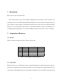
Unofficial Nielsen Lab Manual
January 21, 2015
i
Contents
1
Introduction
3
2
Computational Resources
3
2.1
In-Lab . . . . . . . . . . . . . . . . . . . . . . . . . . . . . . . . . . . . . . . . . . . . . .
3
2.2
Out of Lab . . . . . . . . . . . . . . . . . . . . . . . . . . . . . . . . . . . . . . . . . . . .
3
2.3
Environment . . . . . . . . . . . . . . . . . . . . . . . . . . . . . . . . . . . . . . . . . . .
4
2.3.1
Logging On - In Lab . . . . . . . . . . . . . . . . . . . . . . . . . . . . . . . . . .
4
2.3.2
Terminal-Working from Command Line . . . . . . . . . . . . . . . . . . . . . . . .
4
2.3.3
Terminal Commands . . . . . . . . . . . . . . . . . . . . . . . . . . . . . . . . . .
5
2.3.4
Remote Logging . . . . . . . . . . . . . . . . . . . . . . . . . . . . . . . . . . . .
8
2.4
Text Editors . . . . . . . . . . . . . . . . . . . . . . . . . . . . . . . . . . . . . . . . . . . 10
2.4.1
2.5
Launching Jobs on bigbird - The Job Queue System . . . . . . . . . . . . . . . . . . . . . . 12
2.5.1
3
4
Current Job Queue System . . . . . . . . . . . . . . . . . . . . . . . . . . . . . . . 12
Simulation Codes
13
3.1
LAMMPS . . . . . . . . . . . . . . . . . . . . . . . . . . . . . . . . . . . . . . . . . . . . 13
3.2
NAMD . . . . . . . . . . . . . . . . . . . . . . . . . . . . . . . . . . . . . . . . . . . . . 15
3.3
MPDyn . . . . . . . . . . . . . . . . . . . . . . . . . . . . . . . . . . . . . . . . . . . . . 16
3.4
Other Simulation Codes . . . . . . . . . . . . . . . . . . . . . . . . . . . . . . . . . . . . . 17
Molecular Modeling Codes
4.1
5
VI Usage . . . . . . . . . . . . . . . . . . . . . . . . . . . . . . . . . . . . . . . . 11
17
VMD . . . . . . . . . . . . . . . . . . . . . . . . . . . . . . . . . . . . . . . . . . . . . . 18
Plotting Software
19
5.1
Gnuplot . . . . . . . . . . . . . . . . . . . . . . . . . . . . . . . . . . . . . . . . . . . . . 19
5.2
Xmgrace . . . . . . . . . . . . . . . . . . . . . . . . . . . . . . . . . . . . . . . . . . . . . 20
1
6
7
8
Other Useful Programs, Applications, and Tools
6.1
pdflatex . . . . . . . . . . . . . . . . . . . . . . . . . . . . . . . . . . . . . . . . . . . . . 21
6.2
POV-Ray . . . . . . . . . . . . . . . . . . . . . . . . . . . . . . . . . . . . . . . . . . . . 21
6.3
GIMP . . . . . . . . . . . . . . . . . . . . . . . . . . . . . . . . . . . . . . . . . . . . . . 22
6.4
tmux . . . . . . . . . . . . . . . . . . . . . . . . . . . . . . . . . . . . . . . . . . . . . . . 23
6.5
Mathematica . . . . . . . . . . . . . . . . . . . . . . . . . . . . . . . . . . . . . . . . . . 24
6.6
MATLAB . . . . . . . . . . . . . . . . . . . . . . . . . . . . . . . . . . . . . . . . . . . . 25
6.7
Office Suite . . . . . . . . . . . . . . . . . . . . . . . . . . . . . . . . . . . . . . . . . . . 26
Programming Languages and Resources
26
7.1
Tcl . . . . . . . . . . . . . . . . . . . . . . . . . . . . . . . . . . . . . . . . . . . . . . . . 27
7.2
Bash . . . . . . . . . . . . . . . . . . . . . . . . . . . . . . . . . . . . . . . . . . . . . . . 27
7.3
C++ . . . . . . . . . . . . . . . . . . . . . . . . . . . . . . . . . . . . . . . . . . . . . . 27
7.4
Python . . . . . . . . . . . . . . . . . . . . . . . . . . . . . . . . . . . . . . . . . . . . . . 28
7.5
Fortran . . . . . . . . . . . . . . . . . . . . . . . . . . . . . . . . . . . . . . . . . . . . . . 28
7.6
LaTeX . . . . . . . . . . . . . . . . . . . . . . . . . . . . . . . . . . . . . . . . . . . . . . 28
Simulation Techniques
8.1
9
20
29
Molecular Dynamics . . . . . . . . . . . . . . . . . . . . . . . . . . . . . . . . . . . . . . 29
Coordinate Files
31
9.1
PDB . . . . . . . . . . . . . . . . . . . . . . . . . . . . . . . . . . . . . . . . . . . . . . . 31
9.2
XYZ . . . . . . . . . . . . . . . . . . . . . . . . . . . . . . . . . . . . . . . . . . . . . . . 33
10 Lab Safety
34
10.1 Equipment Safety . . . . . . . . . . . . . . . . . . . . . . . . . . . . . . . . . . . . . . . . 34
10.2 Personal Safety . . . . . . . . . . . . . . . . . . . . . . . . . . . . . . . . . . . . . . . . . 34
10.3 Other Safety Resources . . . . . . . . . . . . . . . . . . . . . . . . . . . . . . . . . . . . . 35
2
1
Introduction
Hello, and welcome to the Nielsen Lab!
Our research group is a part of the Chemistry Department in the University of Texas at Dallas, and
specifically we are located at BE 3.304 in the Berkner building. We are theoretical and computational group
and as such the strongest chemical you will find in the Nielsen lab is coffee. This is an unofficial lab manual
intended to act as an introduction and reference to computational chemistry software and techniques. It is
ever changing and being updated, so if you feel something is missing, don’t hesitate to add to or change it.
2
2.1
Computational Resources
In-Lab
There are currently 5 machines in the lab. They are listed below:
Name
bert
cvc
animal
piggy
grover
Processor
Xeon
Xeon
core 2
quad core
pentium D
Number of CPUs
16
24
2
4
2
Architecture
64-bit
64-bit
64-bit
64-bit
64-bit
Table 1: List of machines available in the lab.
2.2
Out of Lab
The lab also has access to a CPU cluster for more computationally intensive simulations/programs. However,
the cluster is not physically located in the lab and must be accessed through remote logging. The master node
of this cluster is named bigbird and is a 64-bit machine. bigbird has 24 on-board CPUs along with a Tesla
3
scientific grade GPU (Graphics Processing Unit). The additional CPUs in the cluster are partitioned into 4
nodes (b1, b2, b2, and b4) each with 32 cpus. Each node can be logged into directly and have programs/jobs
run or can have jobs partitioned to them from bigbird using the job queue system.
2.3
Environment
All the machines use Linux. The Linux implementation depends on the machine, but the computer network
has been setup so you can log into any machine in the Nielsen lab and still have your files preserved. In
this sense it does not matter which machine you use. You can also remotely log in to and use any other lab
machine from whichever machine you are at. All the machines currently available are 64-bit, so any self
compiled programs should run on any machine in the lab. Before being able to log into the network, you
need to fill in some paperwork for UTD to create an account, which usually takes several weeks (or even
months sometimes). During this time you will most likely use another lab member’s account. If this is the
case, then your host will need to log in for you to have access to lab machines.
2.3.1
Logging On - In Lab
If the machine is off, just turning it on will (after a good 15 minutes some-times) take you to a log in screen.
Your username will usually be your netid. After entering the userid, enter your password to log into the
NSM system. All the machines in the lab work on this system, and every machine will log into your home
directory in the NSM network. For example, a user John B. Smith with a user id of ’jbs072000’ will have a
home directory located on the NSM network:
/net/uu/nm/cm/jbs071000
Once logged onto the machine, you can use Linux much like any windows machine.
2.3.2
Terminal-Working from Command Line
You will often run commands from the terminal. The terminal is just a place where you can type in commands, and display some information. The terminal usually can be started from the system tools using:
4
Panel ⇒ Applications ⇒ System Tools ⇒ Terminal.
The terminal will allow you to do things such as navigate through your directories(folders), display file
contents, move/copy data/files, and execute programs.
2.3.3
Terminal Commands
The terminal is an input/output source where you can type in commands and display information. The
more used to the system you become, the more you start using the terminal, as it allows quick access
commands to manipulate files, directories, and also show information. The complete list of Linux terminal
commands can be found at http://ss64.com/bash/. Usually only a handful of commands are needed
to start working on a terminal, and a list of the most commonly used ones are given below( from http:
//www.unixguide.net/linux/linuxshortcuts.shtml):
< T ab >
<↑>
< Ctrl > c
< Ctrl > z
< M iddleM ouseButton >
∼ (tilde)
.(dot)
.. (two dots)
Table 2: Terminal Usage Shortcuts:
(In a text terminal) Auto-complete the command if there is only
one option, or else show all the available options. THIS SHORTCUT IS GREAT! It even works at LILO prompt!
Scroll and edit the command history. Press < Enter > to execute previous commands.
Kill the current process (mostly in the text mode for small applications).
Send the current process to the background.
Paste the text which is currently highlighted somewhere else.
This is the normal ’copy and paste’ operation in Linux.
My
home
directory
(normally
the
directory
’/home/myloginname’. For example, the command ’cd /mydir’
will change my working directory to the subdirectory ’mydir’
under my home directory. Typing just ’cd’ alone is an equivalent
of the command ’cd’.
Current directory. For example, ’./myprogram’ will attempt to
execute the file ’myprogram’ located in your current working directory.
Directory parent to the current one. For example, the command
’cd ..’ will change my current working directory one one level up.
5
Table 3: Terminal Usage Commands
Command
pwd
Action/Usage
Print working directory, i.e., display the name of my current directory on the screen.
df -h
(=disk free) Print disk info about all the file systems (in humanreadable form)
du/ -bh | more
(=disk usage) Print detailed disk usage for each sub-directory
starting at the ’/’ (root directory(in human legible form).
ls
List the content of the current directory. Under Linux, the command ’dir’ is an alias to ls. Many users have ’ls’ to be an alias to
’ls -color’.
cd < directory >
Change directory. Using ’cd’ without the directory name will
take you to your home directory. ’cd -’ will take you to your
previous directory and is a convenient way to toggle between two
directories. ’cd ..’ will take you one directory up.
cp < sourcedestination >
Copy files. E.g., ’cp /home/stan/existingfilename .’ will copy
a file to my current working directory. Use the ’-r’ option (for
recursive) to copy the contents of whole directories, e.g. , ’cp -r
myexisting/dir/’ will copy a sub-directory under my current working directory to my home directory.
mv < source >< destination >
Move or rename files. The same command is used for moving
and renaming files and directories.
Continued on next page...
6
Table 3 – continued from previous page...
rm < f iles >
Remove (delete) files. You must own the file in order to be able
to remove it. On many systems, you will be asked for confirmation of deletion, if you don’t want this, use the ’-f’ (=force)
option, e.g., ’rm -f *’ will remove all files in my current working
directory, no questions asked.
mkdir < directory >
Make a new directory.
rmdir < directory >
Remove an empty directory.
rm -r files
(recursive remove) Remove files, directories, and their subdirectories. Careful with this command as root-you can easily
remove all files on the system with such a command executed on
the top of your directory tree, and there is no undelete in Linux
(yet). But if you really wanted to do it (reconsider), here is how
(as root): ’rm -rf /*’
cat filename | more
View the content of a text file called ’filename’, one page a time.
The ’|’ is the ’pipe’ symbol (on many American keyboards it
shares the key with ’.́ The pipe makes the output stop after each
screenful. For long files, it is sometimes convenient to use the
commands ’head’ and ’tail’ that display just the beginning and
the end of the file. If you happened to use ’cat’ on a binary file
and your terminal displays funny characters afterwards, you can
restore it with the command ’reset’.
tar -zxvf < f ilename.tar.gz >
(=tape archiver) Untar a tarred and compressed tarball (*.tar.gz or
*.tgz) that you downloaded from the Internet.
Continued on next page...
7
Table 3 – continued from previous page...
top
Keep listing the currently running processes, sorted by cpu usage
(top users first). In KDE, you can get GUI-based Ktop from ’K’
menu under ’System ⇒ Task Manager’ (or by executing ’ktop’ in
an X-terminal).
ps
(=print status) Display the list of currently running processes with
their process IDs (PID) numbers. Use ps axu to see all processes
currently running on your system (also those of other users or
without a controlling terminal), each with the name of the owner.
Use ’top’ to keep listing the processes currently running.
kill PID
Force a process shutdown. First determine the PID of the process
to kill using ps.
2.3.4
Remote Logging
Often you will want to use bigbird to run programs, simulations, etc. You can log onto bigbird using the
terminal. Once the terminal is opened you should see your username (John for example logged onto animal)
:jbs072000@animal;
At this point you can log onto bigbird by entering the following command into the terminal,
:jbs072000@animal; ssh -X -Y [email protected]
8
Which should give the follwing output:
University of Texas at Dallas
Natural Sciences and Mathematics
Pursuant to Texas Administrative Code 202:
Unauthorized use is prohibited;
Usage may be subject to security testing and monitoring;
Misuse is subject to criminal prosecution; and
No expectation of privacy except as otherwise provided by
applicable privacy laws.
[email protected]’s password:
At which point enter your password and the login will be complete. The terminal can also be used to
log onto other machines in the lab, which is useful if you need to run a job or program on a computer that is
not being used. The same process used to log onto bigbird can be used to log onto the computers in the lab,
e.g:
:jbs072000@animal; ssh -X -Y jbs072000@< computername >
will log you into any computer in the lab. There is also a shortcut version of the command that can be used
for the in-lab computers, which is:
:jbs072000@animal; ssh < computername >
The system can also be remotely accessed outside of the campus. You will need a computer with a terminal
from which you can log in. To log onto bigbird requires the same command as in the earlier bigbird example.
However, the NSM system is accessed by using:
9
:john@home; ssh -X -Y [email protected]
Once you are logged onto apache you can then remotely log into any of the other in-lab machines such
as piggy, bert, etc. If you want to access the lab computers or file system from a remote Windows machine
it is helpful to use a terminal emulator. A free and easy to use terminal emulator for Windows systems is
PuTTY (http://www.putty.org/). Otherwise, the system should be accessible through the Windows
remote desktop/logging utility.
2.4
Text Editors
Most of the configuration files and initial coordinate files of simulations are stored in text files. Scripts,
program source codes, and data/output files are also typically stored in text files. To modify or create these
types of files you will need to use a text editor. The choice of editor is personal preference, some options
are given below:
• Vim
• GEdit
• Emacs
From this list, Vim is a terminal program, and editing text is very quick, but VIM does not allow the
use of the mouse to move the cursor. Vim is very powerful but cryptic. The shortcuts which quicken and
simplify life need to be learnt and so typically has the largest initial learning curve. Vim is standard to
many linux distributions, and can be launched by typing ’vi’ in the terminal. To learn more about Vim
visit the Vim website(http://www.vim.org/). Gedit is the gnome/linux equivalent of windows Wordpad. Gedit is typically the easiest to use and get started with. It is considered to be the least powerful of
the listed editors. However, Gedit does allow syntax coloring, bracket matching, line numbering, etc. It
is often a good choice for scripting/latex writing etc. With the use of plug-ins gedit can be extended into
10
a more powerful editor. gedit is launched by either the menu or through the terminal by entering ’gedit’.
To read more about gedit visit the gedit website(https://projects.gnome.org/gedit/). Emacs
is a platform independent program which has a huge following. Another program which is omnipotent,
and can be used to do all of the things that gedit can do and a lot more including compiling and linking programs etc. Emacs is also launched by either the menu (Application ⇒ Acessories ⇒ Emacs Text
Editor) or through the terminal with the ’emacs’ command. To learn more about Emacs visit the Emacs
website(http://www.gnu.org/software/emacs/). The use of Emacs and gedit are much more
intuitive, but the use of vi is not, so a separate section is dedicated to its use.
2.4.1
VI Usage
To edit a text file in VI, launch VI passing the text file as an argument, e.g. to edit a file myfile.txt use:
:jbs072000@animal; vi myfile.txt
This should take you into a blank screen, which is actually in the VI program. VI has a few modes, it
loads into ’Command Mode’ which is progressively more useful the more VI commands you use. To use
VI like a conventional text editor press the ’Insert’ key once, and the status line at the bottom of the screen
should turn into 0 − −IN SERT − −0 which lets you know that you are in ’Insert Mode’ where you can
type things in. Once you have finished typing or editing you can exit by going back into the ’Command
Mode’ by pressing < ESC > and, then save and exit using < SHIF T > +zz. As in most of the
Linux environments, you can copy-paste by highlighting using the mouse and and then pressing down on
the scroll wheel of the mouse or the left and right mouse buttons together at the target position. A word
of caution, VI must be in ’Insert Mode’ to paste text, otherwise it will execute commands corresponding to the pasted text, which may have undesired results. VI is extremely powerful, and can replace text,
search for strings and promote world peace if you learn the commands. A useful PDF cheat-sheet is at
http://www.atmos.albany.edu/deas/atmclasses/atm350/vi_cheat_sheet.pdf. A
few useful commands are given below as well:
11
Command
:q!
:u
:dw
:9 dd
:9
:< SHIF T > g
:%s%apple%pear%g
2.5
Result
Quit without saving changes
Undo last command
Delete word
Delete 9 lines. Any number of lines is allowed
Move cursor to line number 9. Any line number is allowed
Move cursor to last line in file
Replaces all occurrences of text ’apple’ with ’pear’ in the file
Launching Jobs on bigbird - The Job Queue System
To launch large jobs or jobs with many simulations on the cluster (bigbird) it is useful to send the jobs
through the job queue system. The job queue system manages the computing resources on the cluster and
allows jobs to be lined up (queued) and run automatically when the appropriate numbers of CPUs become
available.
2.5.1
Current Job Queue System
The job queue system that is currently on bigbird is SLURM (https://computing.llnl.gov/
linux/slurm/). SLURM stands for Simple Linux Utility for Resource Management and is an open
source resource management system. The most useful and basic commands will be covered here but more
extensive resources can be found in the SLURM documentation at https://computing.llnl.gov/
linux/slurm/documentation.html.
The most basic command to launch jobs is the ’srun’ command.
Example : srun job binary
There are also command line options and flags that can be used when launching jobs with SLURM. The
three basic resource request flags are given in the Table 4.
Once jobs have been submitted you can check the queue status with command ’squeue’. squeue will list
all jobs that have been submitted to the queue system along with useful information about the job’s status.
12
Flag
-N
-n
-c
Use
Number of nodes requested
number of tasks to run on each node
number of cpus per task
Table 4: An example use of srun with the flags is ’srun -N1 -n1 -c8 job binary’ where the job is sent into
the queue requesting that one node be used with one task and eight CPUs for that task.
3
Simulation Codes
There a couple of MD simulation programs that are most often used in the lab. These include LAMMPS
and NAMD. Another simulation program that can perform MD named MPDyn is also available for lab use.
Although use of MPDyn in the lab has declined over the past few years, it is still a powerful simulator and
worth mentioning.
3.1
LAMMPS
Figure 1: Image of AFM tip surface deformation simulation run using LAMMPS.
LAMMPS stands for Large-scale Atomic/Molecular Massively Parallel Simulator. It is a classical MD code
originally developed by and now distributed by Sandia National Labs. LAMMPS contains a large variety of
13
functionality and is open source, so can be extended by the user. LAMMPS can be run on a single processor
or in parallel using some form of message passing, e.g. Message Passing Interface(MPI). LAMMPS can
also be compiled with GPU accelerated functions. The most current source code for LAMMPS is written in
C++. More information about LAMMPS including links to the user manual, tutorials, a full list of standard
LAMMPS commands, and more, can be found at the LAMMPS web site(http://lammps.sandia.
gov/).
14
3.2
NAMD
Figure 2: Image from simulation of osmotic water transport through CNTs embedded in a membrane run
with NAMD
NAMD is the acronym for Not (just) Another Molecular Dynamics (simulation package). NAMD has been
developed namely for use in simulating large bio-molecular systems or systems with large numbers of atoms.
NAMD is capable of running massively in parallel or on single processors. NAMD contains a lot of built-in
functionality written using a Charmm++ programming model. NAMD has been developed jointly by the
Theoretical and Computational Biophysics Group (TCB) and the Parallel Programming Laboratory (PPL)
at the University of Illinois at Urbana-Champaign and is currently distributed by the TCB. NAMD is free to
15
download and is open source. Although, to download NAMD you must create an account with the TCB and
agree to the licensing terms. Links to more information and resources can be found at the TCB’s NAMD
web page(http://www.ks.uiuc.edu/Research/namd/).
3.3
MPDyn
Figure 3: Image from simulation of PEG functionalized nanoparticles at an oil/water interface run using
MPDyn.
MPDyn (assumedly Molecular/Particle Dynamics, although this is just a guess) is a simulation program
developed by Watura Shinoda out of the Nanosystem Research Institute at the National Institute of Advanced Industrial Science and Technology (AIST) in Japan. Dr. Shinoda is a personal friend and long
time collaborator of Dr. Nielsen’s. MPDyn has been devoloped primarily for macro-molecular systems
16
(e.g. biological membranes). MPDyn can do standard Molecular Dynamics simulations, but can also
do other simulation methods including Hybrid Monte-Carlo, Dissipative Particle Dynamics, Path Integral
Molecular Dynamics, and Centroid Molecular Dynamics. The MPDyn homepage is located at https:
//staff.aist.go.jp/w.shinoda/MPDyn/.
3.4
Other Simulation Codes
LAMMPS, NAMD, and MPDyn are the most commonly used MD programs in the lab, but there are many
other simulation packages available that may be encountered. Just a few are listed below:
• CHARMM - Molecular Dynamics: http://www.charmm.org/
• Amber - Molecular Dynamics: http://ambermd.org/
• xplor-nih - Structure Determination: http://nmr.cit.nih.gov/xplor-nih/
• Jaguar - Ab Initio Electronic Structures:http://www.schrodinger.com/productpage/14/7/
Of course, the above is by no means a comprehensive list. There are a myriad of simulation codes that
use various methods and often are geared for specific applications. However, a much more comprehensive
list of Molecular Mechanics and Molecular Modeling software is available at the Wikipedia page athttp:
//en.wikipedia.org/wiki/List_of_software_for_molecular_mechanics_modeling
4
Molecular Modeling Codes
”Molecular Modeling Code” may seem like another good name for simulation codes, but to differentiate, a
molecular modeling code is software in which the predominate function is visualization. i.e. these types of
software are used to look at, build, and often analyze the structures (e.g. molecules, atom configurations, or
any other simulated system) that are used/generated in simulations. Molecular modeling codes are very useful and are often quite powerful; usually containing extensions to, in many cases, to perform structure refinement, simple simulations, and many other things. The visualization program that is most often used in the lab
17
is called VMD. Another popular molecular modeling software is called Maestro. Maestro is developed and
distributed by the company Shrödinger (like the equation) and can be downloaded for free under an academic
liscence. The associated webpage is http://www.schrodinger.comproductpage/14/12/
4.1
VMD
Figure 4: Image of surfactant peptides interaction with a carbon nanotube in water generated by VMD.
VMD or Visual Molecular Dynamics is a powerful molecular modeling program primarily for displaying,
animating, and analyzing molecular systems. VMD is the choice modeling program of the lab. It is developed and distributed by the TCB (Theoretical and Computational Biophysics Group) at the University of
Illinois Urbana-Champaign. It is a companion program to NAMD but, does not require NAMD, except to do
real-time interactive NAMD simulations, and can be used to visualize many different coordinate/trajectory
file types from different simulation codes. VMD uses 3-D graphics and offers many extensions and functions. The code is free to download and is open source. VMD supports a scripting interface in both TcL
(Tool Comand Language) and Python languages. VMD has a large library of scripting functions built-in
18
which can be used in conjunction with the normal Tcl/Python commands. The scripting interface allows
users to write their own functions and small programs to run within VMD to do all sorts of various tasks.
As mentioned, scripting in VMD can be used for many things, but is probably most commonly used (within
the lab) for analysis of simulation systems and trajectories. For more information, path to downloads, links
to tutorials, and more, visit the VMD web page at http://www.ks.uiuc.edu/Research/vmd/
5
Plotting Software
Data generated in the lab often requires some form work up (such as further processing, etc.), but a crucial
application is plotting data to generate charts, graphs, figures, etc. The two main graphing applications used
in the lab are gnuplot and xmgrace.
5.1
Gnuplot
Figure 5: Plot generated using Gnuplot.
Gnuplot is a command line graphing utility. It is typically run in a terminal and can be started by typing
the ’gnuplot’ command. Gnuplot is capable of generating both 2-D and 3-D plots. It’s command line style
makes for quick use and is often used in the lab to examine data ”on the fly,” although Gnuplot is capable of
generating publication quality figures. In the lab, Gnuplot is the primary progam used to generate 3-D plots
and quick 2-D plots. To find out more about Gnuplot visit the website at http://www.gnuplot.info/
19
5.2
Xmgrace
Figure 6: Plot of nanoparticle solvation free energies generated using Xmgrace.
Xmgrace or just Grace is a GUI (Graphical User Interface) plotting program for generating 2-D plots.
Xmgrace has many other features besides just plotting, e.g. data integration, histogram, curve fitting, etc.
Xmgrace is the lab choice for generating publication quality 2-D plots. Xmgrace can be started from the
terminal using the ’xmgrace’ command. To learn more and find links to downloads and useful information,
visit the Grace website at http://plasma-gate.weizmann.ac.il/Grace/
6
Other Useful Programs, Applications, and Tools
In addition to simulation, modeling, and plotting software, there are many other programs, applications, and
tools that are available and (are/can be) used in the lab. Some of these are discussed below.
20
6.1
pdflatex
pdflatex is a program that allows you to compile LaTeX code (see Section 7.6) into PDF (Portable Document
Format) files. pdflatex can be executed from the terminal using ’pdflatex filename.tex’ and will generate a
file named filename.pdf. To learn more visit
http://www.math.rug.nl/$\sim$trentelman/jacob/pdflatex/pdflatex.html
6.2
POV-Ray
Figure 7: Image of a simulation system generated using POV-Ray.
POV-Ray or the Persistence of Vision Raytracer is a free tool used to create high quality 3-D graphics. It
has been used much in the lab to generate publication quality images (some of which have even made book
covers). POV-Ray is quite powerful, but is not a GUI program. It is a code interpreter, i.e., you write POVRay code and then compile the code to generate images. To compile POV-Ray code from the terminal use the
21
’povray filename.pov’ command. To learn more, access sample images, downloads, POV-Ray commands,
and tutorial links, visit the POV-Ray site athttp://www.povray.org/
6.3
GIMP
Figure 8: Screenshot of open GIMP window displaying a GIMP genrated image.
The GNU Image Manipulation Program or GIMP is a free GUI software for image creation and manipulation. It is essentially the open source equivalent to Adobe’s Photoshop. GIMP can be quite useful for
transforming image file types, adding content to images, or extracting pictures from screen shots, and more.
GIMP features a large number of drawing tools and supports multi-layering of images. GIMP can typically
be accessed through the panel by ’Applications ⇒ Graphics ⇒ GNU Image Manipulation Program’ or can
be started from the terminal by typing the ’gimp’ command. To learn more about GIMP, visit the website
http://www.gimp.org/
22
6.4
tmux
Figure 9: Screenshot of tmux setup.
tmux is a free open source terminal multiplexer, which allows the user to split terminal window and run
multiple programs or tools at the same time. It allows for easy switching between the windowpanes and
reduces the need for multiple tabs and/or separate instances of the terminal to multi-task. tmux can be very
useful. However, it does require the use of keyboard commands/bindings to navigate and perform tmux
functions. Thus, it takes a little time to get used to working in. For more information, links to the manual,
source code, and more, visit the Source Forge page for tmux at http://tmux.sourceforge.net/
Note: An alternative to tumux is GNU screen, which has many features similar to tmux. To learn more
about GNU screen visit http://www.gnu.org/software/screen/
23
6.5
Mathematica
Figure 10: 3-D plot generated using Mathematica.
Mathematica is very powerful computational program developed by Wolfram. It has many abilities, from
taking derivatives and doing integration to 2-D and 3-D plotting, and much more. Mathematica is a commercial software and is not free. However, UTD has a site license and Mathematica can be used from the
lab computers. To start Mathematica simply use the command ’mathematica’ in the terminal. Mathematica is also available on the computers at the campus library and computing labs. It can also be purchased
at a discounted price from the campus bookstore. To learn more about Mathematica see the website at
http://www.wolfram.com/mathematica/
24
6.6
MATLAB
Figure 11: Plot generated using MATLAB.
MATLAB is another powerful technical computing platform that can be used for numerical computation, visualization, and programming. MATLAB is developed by MathWorks and like Mathematica is
a commercial software that is not free. However, UTD has a site license for MATLAB as well, and
it can be used on the lab computers. To start MATLAB simply type and execute the ’matlab’ command in the terminal. MATLAB is also available on all the campus supported computers and can be purchased at discounted price from the campus bookstore. To learn more about MATLAB visit the website at
http://www.mathworks.com/products/matlab/
25
6.7
Office Suite
The computers in the lab also carry implementations of a free open source office suite. The implementation
may vary depending on the machine, but should either be OpenOffice or LibreOffice. These office suites
contain a word processor, spreadsheet editor, powerpoint editor, and database editor. The environment of
these programs is very similar to that of implementations of Microsoft Office. To access these you can
go through the navigation panel. e.g. ’Applications ⇒ Office ⇒ LibreOffice Writer’ . The office suites
can also be launched from the terminal using either ’openoffice.org’ or ’libreoffice’ commands. To learn
more visit the websites for LibreOffice(http://www.libreoffice.org/) and OpenOffice(http:
//www.openoffice.org/).
7
Programming Languages and Resources
Work in the lab often requires members to write pieces of code, whether it is an analysis script for VMD,
a file manipulation script, or a full fledged program. There are many different programming languages that
each have their strengths and weaknesses. The languages that are currently most commonly used in the lab
are Tcl, Bash, C++, Python, Fortran. Tcl and Bash are higher level programming languages which are
typically used for scripting, while C++ is a lower level language used for writing longer and more powerful
programs. Python has features allowing it to be used for both scripting and more powerful programs. Fortran
is a powerful language for scientific applications. It is a somewhat older language and isn’t used as much
by lab members, but is the preferred programming language of Dr. Nielsen. Therefore, it is useful to at
least become familiar enough to be able to read and make small modifications to Fortran code. Additional
information and links to resources are given in the following subsections for theses languages. However,
there are many many languages that can be used. Some additional choices could be C, C#, Ruby, etc. A more
comprehensive list of programming languages is given on this Wiki page: http://en.wikipedia.
org/wiki/List_of_programming_languages
26
7.1
Tcl
Tcl or Tool Command Language is higher level programming language. It is often used as an embedded
scripting interface in large programs through the use of the Tk console, but is not limited to such applications. VMD uses Tcl and the Tk console as the primary scripting interface. It is highly recommended that
lab members become familiar with using Tcl for scripting in VMD (although VMD does offer a Python
interpreter, making Python a viable alternative Tcl in VMD scripting). Some more information can be
found at the following sites: http://tcl.sourceforge.net/ and http://www.tcl.tk/ . The
VMD user guide has a large section that covers scripting in VMD, which can be referenced for learning
VMD specific functions and examples. The download links to the user guide for VMD can be found at
http://www.ks.uiuc.edu/Research/vmd/current/docs.html
7.2
Bash
Bash or the Bourne Again Shell is a free Unix shell. Bash serves as a command processor from the terminal and can also be written into scripting files. It allows for the manipulation of files, data, launching of programs, launching of simulations, etc. Bash scripting can be used to make many things much
more efficient, e.g. extracting a single line from a set of data files and parsing into a single file. Lab
members are highly encouraged to become familiar with Bash scripting. For some more resources regarding Bash see the sites at http://www.gnu.org/software/bash/manual/bashref.html and
http://www.tldp.org/LDP/abs/html/
7.3
C++
C++ is a low level object-oriented programming language used to write many large and powerful programs (e.g. VMD and LAMMPS are written in C++). C++ is a superset (although, not necessarily
a strict superset) of the C programming language. Although there are many options for choosing a primary programming language, C++ is a widely used and powerful language, and is the recommended
choice of programming language for lab members to learn. An excellent C++ resource can be found at
27
http://www.cplusplus.com/
7.4
Python
Python is an interpreted language. Python has many features and libraries which make it usesful for both
high level scripting or lower level programming. Due to its relative ease of use and growing popularity it
is a good introductory programming language. Many useful resources for Python can be found at https:
//www.python.org/
7.5
Fortran
Fortran is powerful low level programming language that was developed especially for numerical and scientific computing. Although originally developed in the 1950s Fortran remains widely in use for numerically intensive computations. One source of information and tutorials can be found at http://www.
fortran.com/the-fortran-company-homepage/fortran-tutorials/.
7.6
LaTeX
LaTeX is free document preparation system with many features designed for technical and scientific writing.
It is quite powerful and includes many features which make scientific writing much cleaner and often much
easier. It is thus commonly used in the lab for writing articles, book chapters, etc. (e.g. The source for this
manual was written in LaTeX) LaTeX is a programming style language, i.e. the user writes code in LaTeX
which is then compiled to generate the actual document( e.g. with pdflatex (section 6.1) to generate a pdf
document.). To learn more about LaTeX see the website at http://www.latex-project.org/
28
8
8.1
Simulation Techniques
Molecular Dynamics
Molecular dynamics is a computer simulation method where we study the movement of atoms and molecules.
Conventionally this is classical mechanics method (i.e. we do not use quantum mechanics) where the force
acting on each atom is calculated through the application of Newtons laws. The instantaneous force and
hence the resulting velocities of the atoms are computed and through using time-integrator the atoms are
moved accordingly over a discrete time-step. It is assumed that the forces acting on the atoms do not change
during this time step and hence the time step is necessarily small, in the femto second range (10−15 s).
The computer does this loop continuously, updating the force and velocity of each atom then updating their
positions to obtain a trajectory of the system.
The information contained in the trajectory allows the calculation of thermodynamic quantities such as
free energies, partition co-efficients, diffusion constants, etc. Apart from measuring quantities, molecular
dynamics allows us to have a microscope of infinite resolution ( because Heisenberg has no say here! ) and
see physical processes occurring at the molecular scale.
The main limitation on molecular dynamics is that electronic structure of atoms is treated explicitly,
hence it is not a good method to study systems where there is rearrangement of electrons such as chemical
reactions where covalent bonds are formed, redox reaction etc. Although newer molecular dynamics have
been developed to allow simulation of systems with explicit electron rearrangement, the majority of simulation studies are carried out on physical phenomena.
A concept central to the ability to calculate the forces acting on atoms through a classical mechanics
frame work is that of a force field. The force field decomposes the structure-energy relationship of molecules
and atoms into several components, both bonded and non-bonded. In essence the force field gives us a way
29
to calculate the energy of the system as a function of the spatial coordinates (positions) of the atoms, usually
through simple mathematical forms.
In general, since the force acting on any particle in a given system depends on all atoms in the system,
the number of calculations needed for one time step increases with N 2 where N is the number of atoms
in the system. Therefore, there is a practical limit to the size of the systems we can look at for how many
time steps we can run the trajectory for. This fact also manifest in a compromise in the details we include in
the atomic description of the molecules in the system and the time it takes to simulate. With conventional
computational systems (in 2011), researchers in the molecular dynamics field often study systems in the
scale of hundreds of nanometers for hundreds of nanoseconds. This is often surprising to people new to the
field who expect the power of computers to be able to accomplish much more, however the sheer number of
interactions that need to be calculated is staggering. Methods have been developed that effectively reduce
the size / speed scaling to N from N 2 , however, this still means that we are dependent on computational
power, or the use of clever methods, which will be discussed later.
The fact that molecular dynamics (MD) is limited in the system sizes it models, we use a simulation
box ( also called a simulation cell ) on a fixed number of atoms. To avoid the problems associated surfaces,
the convention of periodic boundaries are often used, where there are copies of the simulation cell around
it such that an atom moving out of the cell re-appears on the other side. This has the effect of not having
surfaces on the cell edge, which is essential if the system simulated is meant to model a system from a
extended environment, e.g. a solution or cell membrane, etc.
Furthermore, MD techniques have been developed such that we can study systems in different conditions. For an isolated system, the energy of the system is conserved through Newtonian mechanics, and this
ensemble is conceptually the easiest to treat, the N V E ensemble ( constant number of particles, constant
volume, constant energy ). However, by coupling the particles in the simulation cell to a heat bath, we can
30
introduce a constant temperature, and study systems in N V T ensemble. Here the energy of the system can
change, but the temperature remains constant over long periods of time. The N P T ensembly ( constant
composition, pressure and temperature ) can be implemented by also allowing the size of the simulation
cell to vary to maintain the proper pressure within the system. For many chemical system, which are in
atmospheric pressure or within the pressure of the body, this is N P T ensemble or the isothermal-isobaric
ensemble is the one we wish to carry out simulations on.
9
Coordinate Files
Coordinate files are used to store static snapshots of molecular systems. These files include the positions
of all atoms and may include information about the types of atoms. There are various types and formats of
coordinate files that exist. Here we will cover the two most common for use within the lab. These are the
PDB and XYZ format files.
9.1
PDB
The PDB file format stands for Protein DataBase, and is probably the most widely used file format to
save spatial coordinates of systems, especially for biological molecules. The Protein Data Bank, http:
//www.pdb.org/pdb/home/home.do keeps a repository of a large number of proteins which have
been resolved through xray crystallography and other means. A PDB file is also stored as text and therefore
easily editable by hand, which is a major advantage. Below is a snippet from such a file:
Example:
1
2
3
4
5
6
7
8
12345678901234567890123456789012345678901234567890123456789012345678901234567890
ATOM
145
N
VAL A
25
32.433
31
16.336
57.540
1.00 11.92
A1
N
ATOM
146
CA
VAL A
25
31.132
16.439
58.160
1.00 11.85
A1
C
ATOM
147
C
VAL A
25
30.447
15.105
58.363
1.00 12.34
A1
C
ATOM
148
O
VAL A
25
29.520
15.059
59.174
1.00 15.65
A1
O
ATOM
149
CB AVAL A
25
30.385
17.437
57.230
0.28 13.88
A1
C
ATOM
150
CB BVAL A
25
30.166
17.399
57.373
0.72 15.41
A1
C
ATOM
151
CG1AVAL A
25
28.870
17.401
57.336
0.28 12.64
A1
C
ATOM
152
CG1BVAL A
25
30.805
18.788
57.449
0.72 15.11
A1
C
ATOM
154
CG2BVAL A
25
29.909
16.996
55.922
0.72 13.25
A1
C
...
...
...
where the column and the data type are as follows:
• 1 - 6 (Record name) ”ATOM ”
• 7 - 11 (Integer) Atom serial number.
• 13 - 16 (Atom ) Atom name.
• 17 (Character) Alternate location indicator.
• 18 - 20 (Residue name) Residue name.
• 22 (Character) Chain identifier.
• 23 - 26 (Integer) Residue sequence number.
• 27 (AChar ) Code for insertion of residues.
• 31 - 38 (Real(8.3) ) Orthogonal coordinates for X in Angstroms.
• 39 - 46 (Real(8.3) ) Orthogonal coordinates for Y in Angstroms.
32
• 47 - 54 (Real(8.3) ) Orthogonal coordinates for Z in Angstroms.
• 55 - 60 (Real(6.2) ) Occupancy.
• 61 - 66 (Real(6.2) ) Temperature factor (Default = 0.0).
• 73 - 76 (LString(4)) Segment identifier, left-justified.
• 77 - 78 (LString(2)) Element symbol, right-justified.
• 79 - 80 (LString(2)) Charge on the atom.
more information of all the types of entries in pdb files can be found at http://deposit.rcsb.
org/adit/docs/pdb_atom_format.html.
9.2
XYZ
The XYZ type coordinate format is one of the simplest formats and is often used for homegrown code
outputs due to ease. The format follows:
N
comment line
type x y z
type x y z
..........
where N is the total number of atoms. The comment line can be any text. Example:
7
lj particles 7 E: 10.3301
lj 0.430075494380179 -1.373428295207335 2.226047612914703
lj 0.849657136368228 -0.151548730880504 -1.838948144497242
lj -0.501428449094033 1.199095805189036 -2.186086547932692
33
lj -0.752983275021844 1.119587984733615 -0.633645281498183
lj 1.520445534887691 1.100300399013814 0.515246574782138
lj -0.758705888807712 1.042307524638539 1.654059109324302
lj 0.199673872848771 1.180678018594173 1.301612000610540
10
Lab Safety
The Nielsen Lab is not a conventional wet chemistry lab and so does not follow the typical wet laboratory
safety rules. However, the lab has its own safety concerns. These can be loosely categorized into two types:
Equipment Safety and Personal Safety.
10.1
Equipment Safety
Lab members should take care when working with electronic equipment in the lab. This includes (but is
not limited to) power chord and socket safety. Lab members should make sure all power chords are safely
secured such as to prevent tripping. Also, lab members should take care not to overload power sockets and
power strips, as this could cause electrical shorting and may lead to electrical fire. Lab members should also
take care when eating or drinking near the lab equipment, so as to avoid spilling these on keyboards, mice,
etc.
10.2
Personal Safety
Personal safety includes awareness of things such as, posture and ergonomic practices when working at the
computer. A list of ergonomic tips from The UTD Environmental Health and Safety office can be downloaded from http://www.utdallas.edu/ehs/manuals/docs/tips.pdf . Another safety concern for lab members is eye strain caused by long periods of looking at computer monitor screens. A list of
tips to prevent eye strain from the Mayo Clinic is provided at
http://www.mayoclinic.com/health/eyestrain/DS01084/DSECTION$=$prevention
34
10.3
Other Safety Resources
The UTD Environmental Health and Safety department (http://www.utdallas.edu/ehs/) provides many resources to learn about general and work safety. A couple of resources can be downloaded
from:
• www.utdallas.edu/audit-compliance/training/WorkplaceSafety.pdf
• www.utdallas.edu/ehs/manuals/docs/occupationalandgeneralsafety.pdf
35